Itemset Utility Maximization with Correlation Measure

Abstract

As an important data mining technology, high utility itemset mining (HUIM) is used to find out interesting but hidden information (e.g., profit and risk). HUIM has been widely applied in many application scenarios, such as market analysis, medical detection, and web click stream analysis. However, most previous HUIM approaches often ignore the relationship between items in an itemset. Therefore, many irrelevant combinations (e.g., {gold, apple} and {notebook, book}) are discovered in HUIM. To address this limitation, many algorithms have been proposed to mine correlated high utility itemsets (CoHUIs). In this paper, we propose a novel algorithm called the Itemset Utility Maximization with Correlation Measure (CoIUM), which considers both a strong correlation and the profitable values of the items. Besides, the novel algorithm adopts a database projection mechanism to reduce the cost of database scanning. Moreover, two upper bounds and four pruning strategies are utilized to effectively prune the search space. And a concise array-based structure named utility-bin is used to calculate and store the adopted upper bounds in linear time and space. Finally, extensive experimental results on dense and sparse datasets demonstrate that CoIUM significantly outperforms the state-of-the-art algorithms in terms of runtime and memory consumption.

This article contributes to a utility-based correlated pattern discovery method for transaction databases. It studies the relationship between consisted items of a profitable itemset. Compared with the state-of-the-art algorithms, the designed CoIUM method has greatly improved the performance in terms of execution time and memory consumption. The proposed method is good at dealing with massive database, especially dense databases, which is very beneficial to dealing with commodity sales in real life. Based on large-scale testing, it is found that this method has good scalability in terms of runtime and memory consumption, which indicates that CoIUM is suitable for different types of databases (include sparse and dense). Since the traditional high utility itemset mining has been successfully applied in many applications and various domains, this correlated utility mining problem formulation and efficient algorithm can be applied in many applications, such as product recommendation, market basket analysis, e-learning, text mining and web click stream analysis.

Data mining, correlated itemset, high utility itemset, upper bounds.

1 Introduction

Data mining techniques (e.g., pattern mining [1, 2]) play a vital role in many real-life applications, such as market analysis [3] and website click stream analysis [4]. In previous studies on data mining, a fundamental task called frequent itemset mining (FIM) [5, 6, 7] is used to discover itemsets that frequently occur in a transaction database. FP-Growth [6] is one of the most famous FIM algorithms. It maintains the original database in an FP-tree structure [6]. However, the limitation of traditional FIM algorithms is that different items have identical importance (e.g., unit profit or weight). For instance, the profit of a piece of bread is equal to that of a diamond in the FIM domain. This assumption is unrealistic in real business life.

To address the above limitations, a new framework known as high utility itemset mining (HUIM) [8, 9, 10] was proposed. Compared to FIM, HUIM considers both the quantity and profit of an item. An itemset is referred to as a high utility itemset (HUI) if its utility value is higher than or equal to the user-specified minUtil. HUIM has attracted considerable attention in recent decades because discovering profitable patterns is more valuable than discovering frequent patterns for enterprises. In FIM, the support of an item has an anti-monotonic property, which means that the support of an itemset is not less than that of its supersets. This property can efficiently reduce the search space because supersets of infrequent itemsets are not considered. However, the utility of an item in HUIM does not hold this property. For example, in a supermarket, assume that the amount of the daily sales of {bread} is $100, but the amount of daily sales of its supersets (i.e., {bread,milk}) may be less than, equal to, or higher than $100. This indicates that the utility is neither monotonic nor anti-monotonic. To address this issue, transaction-weighted utilization (abbreviated as TWU), which has the anti-monotonic property, was proposed by Liu et al. [11]. Based on the TWU measure, HUIM can prune the search space effectively. After that, a lot of HUIM algorithms [10, 12, 13] adopted TWU to improve their performance. In general, HUIM approaches can be summarized into two types: two-phase and single-phase algorithms. The two-phase algorithms are characterized by discovering HUIs in two steps. In the first step, numerous candidates are generated by overestimating the utility of itemsets. Then, they calculate the real utility of candidates to filter out HUIs. These two-phase algorithms can discover a complete set of HUIs, there are two shortcomings that cannot be ignored: 1) generating many candidates in the first phase; and 2) repeatedly scanning the database. As a result, two-phase algorithms suffer from long execution times and memory consumption. To solve these issues, the first single-phase HUIM algorithm called HUI-Miner [10] was proposed. Compared to the two-phase algorithms, the single-phase algorithms do not need to repeatedly scan the database. The existing single-phase algorithms include: FHM [14], EFIM [15], MEFIM [16], etc.

However, a key disadvantage of HUIM algorithms is that they usually ignore the relationships between items. This case will usually reveal numerous irrelevant items in high-utility itemsets. For example, in market analysis, assume that {notebook, book} and {phone, TV} are high utility patterns. Obviously, these products (i.e., notebook, book, phone) are weakly correlated. Instead, in real life, retailers often hope to earn more revenue by making related products into product combinations, such as {milk, bread}, {gold, diamond}, and {computer, mouse}. In essence, these products have a strong connection because they often meet the needs of most customers. To discover more correlated high utility itemsets (CoHUIs), some interesting measures such as Kulc [17], bond [18] and coherence [19] were proposed as standards. Based on the definition of Kulc, many algorithms like CoHUIM [20], CoUPM [12] and ECoHUPM [21] were adopted to discover CoHUIs. These algorithms improved the mining performance by using novel data structures and pruning strategies. Recently, Vo et al. [22] presented the CoHUI-Miner algorithm. They used projection techniques to reduce the expense of database scanning and utilized several pruning strategies to mine CoHUIs effectively. However, CoHUI-Miner only used loose upper bound (TWU and remaining utility) to prune the search space, which led to numerous unpromising candidates being generated. Therefore, it suffered in terms of runtime and memory consumption.

To this end, we propose an efficient projection-based algorithm, namely Itemset Utility Maximization with Correlation Measure (CoIUM). Compared to other state-of-the-art algorithms, CoIUM can discover a complete set of CoHUIs more effectively with less execution time and memory consumption. The main contributions of our work are as follows:

• We put forward a single-phase algorithm which utilizes two tighter upper-bounds to discover all CoHUIs without candidate generation. Also, the utility-bin structure [15] is adopted to calculate and store the upper bounds of itemsets.

• The CoIUM algorithm uses a projection technique that can effectively prune the search space.

• The CoIUM algorithm adopts a measure called $Kulc$ as the correlation factor. It is used as a metric to distinguish whether items are highly correlated.

• Massive experiments are conducted on several datasets to evaluate the performance of CoIUM. We also compare the performance of CoIUM with the state-of-the-art algorithms. The results show that the CoIUM is the most efficient in terms of runtime and memory consumption.

The rest of this paper is organized as follows. Some related works about HUIM and CoHUIM are introduced in Section 2, respectively. In Section 3, we introduce the preliminaries and problem statement of correlated high-utility itemset mining. In addition, a novel CoIUM algorithm is proposed in Section 4. Several experimental results are presented in Section 5. Finally, the conclusion and future work are presented in Section 6.

2 Related Work

2.1 High Utility Itemset Mining

A key difference between high utility itemset mining (HUIM) [9, 10, 23, 24] and frequent itemset mining (FIM) [6, 7] is that frequency has the anti-monotonic property, but utility does not. Hence, if itemset is unpromising, the HUIM cannot easily filter out all its supersets in advance. To address this limitation, transaction-weight utilization (TWU), which is anti-monotonic, was first proposed in Two-Phase [11]. Based on the TWU measure, if TWU of a subset is lower than a given minUtil threshold, all its supersets are not HUIs [11]. Therefore, almost HUIM algorithms reduce the search space by using the TWU measure. However, TWU is a loose upper bound for eliminating candidates. Thus, this measure always overestimates the utilities of itemsets, which may result in massive candidates. At the same time, IHUP [8] constructed a tree structure to discover HUIs. Compared with Two-Phase, this new structure can save more runtime and memory. Thus, the experimental results showed that IHUP was about three times faster than Two-Phase in runtime. However, the upper bound of IHUP was not tight, which may have retained numerous unpromising candidates. To reduce the generation of unpromising candidates and identify HUIs effectively, Tseng et al. [13] proposed UP-Growth. It also constructed a pattern tree to extract HUIs and utilized several novel strategies to discover HUIs effectively. UP-Growth can reduce the numerous unpromising candidates and enhance mining performance, so it outperformed IHUP in terms of runtime and memory.

The above-mentioned algorithms are two-phase algorithms, and they face the problems of generating numerous unpromising candidates and scanning the database at least twice. To address these shortcomings, a single-phase approach was proposed to discover HUIs. As a single-phase approach, HUI-Miner [10] algorithm utilized a new data structure called utility-list, which can retain key information about HUIs without scanning the database multiple times. HUI-Miner used a depth-first search to discover all HUIs without omission, and constructed the utility-list of each itemset by joining the utility-lists of its subsets. HUI-Miner can reduce numerous candidates because it uses the remaining utility, which is more compact than TWU. As for performance, HUI-Miner is superior to all two-phase algorithms. Meanwhile, another algorithm called $d^{2}$HUP was presented by Liu et al. [25]. HUI-Miner and $d^{2}$HUP were proposed at the same time, but their key pruning strategies are conceptually equivalent. However, using join operations to create utility-lists is time- and memory-consuming. To reduce the expense of join operations, the FHM algorithm [14] used the EUCP strategy to effectively reduce the generation of join operations. The experiments showed that the performance of FHM is up to 6 times faster than that of HUI-Miner. Then, an algorithm called IMHUP was proposed [26], and utilized an indexed list-based structure to discover HUIs without requiring numerous comparison operations. Based on this structure, two techniques were developed to improve mining performance. In addition, ULB-Miner [27] utilized a utility-list buffer structure to store information and introduced a new index segment to access the stored data. Thus, the performance of ULB-Miner is better than that of HUI-Miner and FHM. EFIM [15] utilized two tighter upper bounds to discover the HUIs effectively. Furthermore, it utilized two new techniques (projection technique and transaction merging) to deal with long transactions. The experiments showed that the performance of EFIM is faster than that of HUI-Miner and FHM on spare and dense databases. The above algorithms are devised under the condition that each item in the database has a different positive utility. Then, the FHN algorithm [28] can discover the HUIs with negative unit profit, and Gan et al. [29] proposed a top-$k$ HUIM algorithm to solve the threshold setting issue. To summarize, many utility mining algorithms have been developed to solve practical problems, including on-shelf utility mining [30], and high average-utility itemset mining [31, 32]. Up until now, a lot of HUIM algorithms with various data have been developed, such as high utility association rules [33], HUIM with fuzzy itemsets [34], targeted utility querying [35], HUIM on massive data [36], HUIM on noisy data [37], and HUIM on stream data [38].

2.2 Correlated High Utility Itemset Mining

Most HUIM algorithms aim to discover a complete set of HUIs, but do not consider the relationships between items in an itemset. To find potential and strong affinity patterns, WIP [39] was proposed, which used a weighted confidence measure to generate strong affinity patterns. Besides, there are three other interesting measures for correlation: any-confidence, all-confidence, and bond [40]. These measures are useful in discovering the degree of connection between items. However, these measures cannot be properly applied to databases that contain numerous empty transactions. To solve this problem, a null-transaction invariant [17] measure was proposed. It was a credible measure because it did not consider how many null-transactions appeared in the database. There are five null-(transaction) invariant measures: all-confidence [18], coherence [18], cosine [17], kulczynsky [17], and max-confidence [18]. Compared with previous studies on traditional data mining approaches, the proposed affinity/correlation patterns can mine more useful information efficiently.

To discover more interesting information, Ahmed et al. [40] first proposed a high-utility itemset mining algorithm to discover HUIs with frequency affinity. The HUIPM algorithm utilized a tree structure UFTA to store HUIs and used a pruning strategy to reduce the generation of unpromising candidates. However, the limitation of HUIPM is that it is time-consuming because it has to establish tree nodes and generate lots of candidates. Thus, Lin et al. [41] presented a single-phase algorithm known as FDHUP which uses two data structures called EI-table and FU-tree, to discover correlated itemsets efficiently. The FDHUP utilized three pruning strategies, which were based on RAU (remaining affinitive utility) to prune the candidates. As a result, FDHUP performed better than HUIPM in terms of runtime and memory. FCHM [42] also discovered the correlated high utility itemsets. It has two versions, FCHM_bond depended on bond measure and FCHM${}_{\textit{all-confidence}}$ relied on all-confidence measure. The algorithm used two structures, utility-list and EUCS, to calculate the TWU values. Then, Gan et al. [20] proposed CoHUIM. This algorithm used a projection mechanism to improve the performance of the scanning database and utilized the property of Kulc to prune the unpromising candidates. They also developed the CoUPM algorithm [12], which utilized utility-list structure to store promising itemsets and used Kulc to calculate the support of itemsets. The algorithm also utilized some properties of utility and correlation to effectively explore the search space. Then, Rashad et al. [21] proposed the ECoHUPM algorithm to evaluate the correlation of HUIs. This algorithm used a new data structure named CoUTlist to store utility and support for each itemset. It also introduced three new pruning properties to prune unpromising candidates. Recently, Vo et al. [22] introduced CoHUI-Miner to extract correlated items that provide numerous benefits. This algorithm applied projection technique to reduce the expense of scanning the database and applied the prefix utility of projection technique to compute the utility value. The experiments showed that it was efficient, especially on dense databases.

3 Preliminaries and Problem Formulation

In this section, we present the basic definitions and problem formulation. More definition details can be referred to previous work [22, 12, 15]. Let $I$ = {$i_{1}$, $i_{2}$, $\dots$, $i_{m}$} be a set of $m$ distinct items in a transaction database $\mathcal{D}$ = {$T_{1}$, $T_{2}$, $\dots$, $T_{n}$}, where $n$ is the number of transactions in $\mathcal{D}$. An $k$-itemset is a subset of $I$ which contains $k$ different items. Each transaction consists of some distinct items and has a unique identifier of $T_{c}$ called Tid. Each item $i\in I$ owns an external utility (e.g., unit profit) that is represented by $pr(i)$. And each item $i$ in transaction $T_{c}$ has an internal utility (e.g., purchase quantity) which denoted as $q(i,T_{c})$. In addition, Table 1 is a simple transaction database (the third column is transaction utility) which consists of six distinct items (i.e., $A$, $B$, $C$, $D$, $E$, and $F$), and Table 2 shows the external utilities of all items.

Table 1: A transaction database

Tid	Transaction	Utility
$T_{1}$	($A$,1) ($B$,2) ($C$,2) ($D$,3)	$19
$T_{2}$	($A$,2) ($B$,1) ($E$,3) ($F$,2)	$18
$T_{3}$	($A$,4) ($C$,3) ($E$,2)	$23
$T_{4}$	($A$,3) ($C$,2) ($F$,3)	$17
$T_{5}$	($B$,3) ($C$,4) ($D$,5)	$25
$T_{6}$	($B$,2) ($C$,3) ($D$,3) ($F$,5)	$21
$T_{7}$	($A$,1) ($B$,2) ($C$,2) ($D$,3) ($E$,5) ($F$,2)	$31
$T_{8}$	($C$,2) ($D$,3) ($E$,1)	$13

Definition 1 (Utility of an itemset)

In a transaction $T_{c}$, the utility of an item $i$ is defined as $u(i,T_{c})$ = $pr(i)$ $\times$ $q(i,T_{c})$, where $i\in T_{c}$. Similarly, the utility of an itemset $X$ is denoted as $u(X,T_{c})$ = $\sum_{i\in X\land X\subseteq T_{c}}u(X,T_{c})$. Furthermore, in database $\mathcal{D}$, the utility of an itemset $X$ is denoted as $u(X)$ = $\sum_{X\subseteq T_{c}\land T_{c}\in\mathcal{D}}u(X,T_{c})$.

For example, the utility of item $A$ in transaction $T_{2}$ is $u(A,T_{2})=$ $4 $\times$ 2 = $8. The utility of itemset $\{A,B\}$ in transaction $T_{2}$ is $u(\{A,B\},T_{2})$ = $u(A,T_{2})$ + $u(B,T_{2})$ = $8 + $2 = $10. At the same time, $u(\{A,B\})$ = $u(\{A,B\},T_{1})$ + $u(\{A,B\},T_{2})$ + $u(\{A,B\},T_{7})$ = $8 + $10 + $8 = $26.

Table 2: External utility of each item

Item	$A$	$B$	$C$	$D$	$E$	$F$
Utility($)	4	2	1	3	2	1

Definition 2 (Utility of database)

The utility of a transaction $T_{c}$ is defined as $tu(T_{c})$ = $\sum_{i_{j}\in T_{c}}u(i_{j},T_{c})$, where $i_{j}$ is the $j$-th item in $T_{c}$. Obviously, the total utility of a database $\mathcal{D}$ is the summation of all transactions it contains, where TU = $\sum_{T_{c}\subseteq\mathcal{D}}tu(T_{c})$.

For example, the utility of $T_{1}$ is $tu(T_{1})$ = $u(A,T_{1})$ + $u(B,T_{1})$ + $u(C,T_{1})$ + $u(D,T_{1})$ = $4 + $4 + $2 + $9 = $19. Then, we can calculate the utility of other seven transactions with the same manner. And the total utility of database $\mathcal{D}$ is $167. Based on the transaction-weighted utilization [11], we have TWU($\{A,B\}$) = $tu(T_{1})$ + $tu(T_{2})$ + $tu(T_{7})$ = $19 + $18 + $31 = $68. Table 3 lists TWU of all 1-itemsets.

Table 3: Support and TWU of all 1-itemsets

Item	$A$	$B$	$C$	$D$	$E$	$F$
TWU	$108	$114	$149	$109	$85	$87
Support	5	5	7	5	4	4

There are many measures [40] used to evaluate the correlation between different items, but some of them will be affected by empty transactions. In this paper, we introduce the Kulczynsky measure [17] (abbreviated as Kulc), which is not affected by null transactions.

Definition 3 (Kulc)

The frequency of an itemset $X$ in database $\mathcal{D}$ is the amount of $X$ occurs. We use sup($X$) to represent the frequency of $X$. For an $k$-itemset $X$ = $\{i_{1},$ $i_{2},$ $\dots,i_{k}\}$, its Kulc is defined as follows: Kulc($X$) = $\frac{1}{k}\times\sum_{i_{j}\in X}\frac{\textit{sup}(X)}{\textit{sup}(i_{j})}$.

For example, Kulc({$A,B$}) = $\frac{1}{2}$ $\times$ ($\frac{\textit{sup}(\{A,B\})}{\textit{sup}(A)}+\frac{\textit{sup}(\{A,B\})}{\textit{sup}(B)}$) = $\frac{1}{2}\times(\frac{3}{5}+\frac{3}{5})$ = 0.6. Obviously, the range of Kulc is [0,1] [20]. In fact, Kulc represents the average of frequency, so if Kulc($X$) becomes high, related items in $X$ appear frequently. Compared to other correlation measures, Kulc holds the null (transaction)-invariant property. It is more suitable for applications in different fields because it is independent on database size [20].

Definition 4 (Correlated high-utility itemset)

An itemset $X$ can be assumed as a correlated high utility itemset (CoHUI) when it meets two conditions: (1) $u(X)$ $\geq$ minUtil $\times$ TU; (2) Kulc($X$) $\geq$ minCor, where minCor is a user-defined minimum correlation threshold.

For example, in a database, minUtil and minCor are set to 0.1 and 0.7, respectively. The itemset $\{A,B\}$ is an HUI because the utility of $\{A,B\}$ is not less than minUtil $\times$ TU ($u(\{A,B\})$ = $26 $>$ minUtil $\times$ TU = 0.1 $\times$ $168 = $16.8), but it is not a CoHUI since its Kulc is less than minCor (Kulc({$A,B$}) = 0.6 $<$ 0.7).

Problem formulation: In a transaction database, given two user-specified minimum thresholds (minUtil and minCor), the purpose of CoIUM is to find all CoHUIs that their utilities are greater than minUtil $\times$ TU and their Kulc is higher than minCor.

4 Proposed CoIUM Algorithm

In this section, we present a single-phase algorithm to extract all CoHUIs. Subsection 4.1 discusses several upper bounds and pruning strategies. Subsection 4.2 introduces an effective projection technology to reduce the cost of database scanning. Subsection 4.3 introduces the pseudocode of the CoIUM algorithm. In Subsection 4.4, we use a detailed example to discuss how CoIUM works.

4.1 Several Strategies for Pruning Search Space

The proposed CoIUM employs a depth-first method to explore the search space. Given a set of distinct items $I$, then the search space ($2^{\mid I\mid}$) can be represented as a set-enumeration tree [43]. The algorithm starts with an empty set. To discover all CoHUIs of itemsets $\alpha$, CoIUM recursively appends its extension to $\alpha$ through the $\succ$ order, and this makes $\alpha$ becomes larger. We assume the items $I$ = {$A$, $B$, $C$, $D$, $E$, $F$} and the total order $\succ$ is TWU ascendant order for the running example. Thus, the order is {$E$ $\prec$ $F$ $\prec$ $A$ $\prec$ $D$ $\prec$ $B$ $\prec$ $C$}.

Property 1

Given an itemset $X$, TWU of $X$ is always higher than or equal to its utility (TWU($X$) $\geq$ $u(X)$).

Strategy 1

Based on Property 1, for any itemset $X$, if TWU($X$) $<$ minUtil $\times$ TU, then all supersets of $X$ are low-utility itemsets. Thus, we can remove the low utility itemsets from the search space. Proof details are provided in study [11].

Definition 5 (Extension of an itemset [15])

Consider an itemset $\alpha$, and $E$ ($\alpha$) is represented as its extension according to the $\succ$ order. E($\alpha$) = {$z$ $|$ $z$ $\in$ $I$ $\land$ $z$ $\succ$ $i$, $\forall$ $i$ $\in$ $\alpha$}. Given an $k$-itemset $X$, we denote its extensions $Z$ containing $(k+i)$ items as $i$-extension of $X$.

For instance, consider the database of our running example and an itemset $X$ = {$A$}. The 1-extension of $X$ are {$A,B$}, {$A,C$}, {$A,D$}, and the itemset {$A,B,C$} is called a 2-extension of {$A$}. To prune more unpromising candidates, it is important to use a more compact upper bound to limit the production of unpromising candidates. We present two upper bounds (TWU and re) that have been used in previous work, and introduce two more compact upper bounds (su and lu) used in this work. Using different strategies based on these upper bounds can prune different numbers of candidates. In addition, we introduce the property of Kulc.

Definition 6 (Remaining utility [10])

Given an itemset $X$ in transaction $T_{c}$. We define $\succ$ as a total order on items from $I$. The remaining utility of $X$ in $T_{c}$ is denoted as $re(X,T_{c})$ = $\sum_{i\in T_{c}\land i\succ x\forall x\in X}u(i,T_{c})$.

For example, we select an itemset $\{A,D\}$ from transaction $T_{1}$. Based on TWU ascendant order, items {$B$} and {$C$} appear after itemset $\{A,D\}$. The remaining utility of $\{A,D\}$ is $re(\{A,D\},T_{1})$ = $u(B,T_{1})$ + $u(C,T_{1})$ = $4 + $2 = $6.

Definition 7 (Local utility [15] and subtree utility [15])

Given an item $z$ and an itemset $\alpha$, where $z\in E(\alpha)$. The local utility of $\alpha$ w.r.t. $z$ is defined as $lu(\alpha,z)$ = $\sum_{(\alpha\bigcup\{z\})\subseteq T_{c}\wedge T_{c}\subseteq\mathcal{D}}[u(\alpha,T_{c})+re(\alpha,T_{c})]$. The subtree utility of $\alpha$ and $z$ is defined as $su(\alpha,z)$ = $\sum_{(\alpha\bigcup z)\subseteq T_{c}\wedge T_{c}\subseteq D}[u(\alpha,T_{c})+u(z,T)]$ + $\sum_{i\in T_{c}\wedge i\in E(\alpha\bigcup\{z\})}u(i,T_{c})$.

For example, we select $\alpha$ = {$A$}. The local utility of $\alpha$ and extension item $D$ is $lu(\alpha,\{D\})$ = $(u(\{A\},T_{1})$ + $re(\{A\},T_{1})$ + $u(\{A\},T_{7})$ + $re(\{A\},T_{7}))$ = $19 + $19 = $38. The subtree utility of $\alpha$ and extension item $C$ is $su(\alpha,\{C\})$ = ($u(\{A\},T_{1})$ + $u(\{C\},T_{1})$ + $0) + ($u(\{A\},T_{3})$ + $u(\{C\},T_{3})$ + $0) + ($u(\{A\},T_{4})$ + $u(\{C\},T_{4})$ + $0) + ($u(\{A\},T_{7})$ + $u(\{C\},T_{7})$ + $0) = [$4 + $2] + [$16 + $3] + [$12 + $2] + [$4 + $2] = $45.

Property 2

Given an item $z$ and itemset $\alpha$, where $z\in E(\alpha)$. We get relationship $lu(\alpha,z)\geq u(Z)$, where $Z$ = $\alpha\cup z$.

Strategy 2

Based on Property 2, given an item $z$ and itemset $\alpha$, where $z\in E(\alpha)$. If $lu(\alpha,z)$ $<$ minUtil $\times$ TU, all extensions of $\alpha$ containing $z$ are low-utility in a subtree. This means that the item $z$ should be removed in the search space of $\alpha$. Proof details are provided in study [15].

For example, if the algorithm discovers itemset {$A,B$} having local utility value is less than minUtil $\times$ TU, all extensions of {$A,B$}, e.g., {$A,B,C$} and {$A,B,D$}, can be ignored.

Property 3

Given an item $z$ and itemset $\alpha$, where $z\in E(\alpha)$. The relationship $su(\alpha,z)\geq u(\alpha\bigcup\{z\})$ always holds on. It also applies to $Z$ which is an extension of $\alpha\cup\{z\}$, that is $su(\alpha,z)\geq u(Z)$.

Strategy 3

Based on Property 3, given an item $z$ and itemset $\alpha$, where $z\in E(\alpha)$. If $su(\alpha,z)$ $<$ minUtil $\times$ TU, all extensions of $\alpha$ containing $z$ are low-utility. In the set-enumeration tree, this means that it is unnecessary to explore $\alpha\cup z$ and all of its supersets. Proof details are provided in study [15].

Based on Strategy 2, the unpromising itemsets will be filtered out from the subtrees of an item $\alpha$. To reduce the cost of exploring search space, Strategy 3 is proposed to identify whole subtrees of $\alpha$ which can be extended.

Definition 8 (Primary and secondary items [15])

Given an item $z$ and itemset $\alpha$, where $z\in E(\alpha)$. The $primary$ items of $\alpha$ are given as Primary($\alpha$) = {$z$ $|$ $z$ $\in$ Secondary($\alpha$) $\wedge$ $su(\alpha,z)$ $\geq$ minUtil $\times$ TU}. The secondary items of $\alpha$ are given as Secondary($\alpha$) = {$z$ $|$ $z$ $\in$ $E(\alpha)$ $\wedge$ $lu(\alpha,z)$ $\geq$ minUtil $\times$ TU}. Note that Primary($\alpha$) $\subseteq$ Secondary($\alpha$).

Consider the running example and $\alpha$ = {$A$}. Primary($\alpha$) = $\{B,C\}$, Secondary($\alpha$) = $\{B,C,E\}$. In other words, the prefixes $\alpha$ $\cup$ $B$ and $\alpha$ $\cup$ $C$ should be explored. Furthermore, only the items {$B,C,E$} should be considered as its extensions. To quickly compute the utility of the upper bounds at any time, we use a utility-bin array structure called UA. This structure is initialized with 0 before calculation and can be reused, which greatly reduces memory consumption.

Definition 9 (Utility-bin array [15])

From database $\mathcal{D}$, there is a set of items $I$. The utility value of the item $i$ is stored in the array UA[$i$], and the length of UA is $\mid I\mid$.

Using UA to calculate lu($\alpha$). First, we initialize the UA by filling all elements with 0. Second, the utility-bin array UA[$i$] is updated as UA[$i$] = UA[$i$] + $u(\alpha,T_{c})$ + $re(\alpha,T_{c})$, where $i\in T_{c}\bigcap E(\alpha)$. After database scanning, $\forall i\in E(\alpha)$, UA[$i$] = lu($\alpha$,$i$).

Using UA to calculate su($\alpha$). First, we initialize the UA by filling all elements with 0. Second, the utility-bin array UA[$i$] is updated as UA[$i$] = UA[$i$] + $\sum_{I\in T_{c}\wedge I\in E(\alpha\bigcup i)}u(I,T_{c})+u(\alpha,T_{c})+u(i,T_{c})$, where $i\in T_{c}\bigcup E(\alpha)$. After database scanning, $\forall i\in E(\alpha)$, UA[$i$] = su($\alpha$,$i$).

The above pruning strategies are based on the upper bounds to prune the space. Next, we will introduce the relevant strategies on the correlation.

Property 4

For any itemset $X\in I$, assume $Y$ is an $k$-extension itemset of $X$, where $k\geq 1$. If $X$ is a related pattern, its extension $Y$ is also a related pattern. The $Kulc$ measure is anti-monotonic: Kulc($Y$) $\leq$ Kulc($X$).

Strategy 4

Based on Property 4, assume that the symbol $\succ$ is sorted in TWU ascending order. When utilizing the depth-first search strategy in the search space, if the Kulc value of any itemset $X$ is less than the minCor value, any of its extension will be regarded as unpromising and irrelevant itemset. They are not CoHUIs which will be ignored. Proof details are provided in the study [12].

For example, set minCor = 0.7, but the Kulc of an itemset $\{A,B\}$ is 0.6. Thus, all its supersets cannot be CoHUIs, and we can remove them from the search space. This anti-monotonic property of Kulc is also known as the sorted downward closure property. In other words, if an itemset $X$ is not a strongly related itemset, all its supersets will also not be strongly correlated itemsets.

4.2 Projection Technology

The CoIUM algorithm employs a projection technique to reduce the memory overhead. When an itemset $\alpha$ is considered extensible, the algorithm only needs to calculate the utility of $E(\alpha)$. And other items which are not belonged to $E(\alpha)$ will be pruned. The database without these items ($i\notin E(\alpha)$) can be called projected database. Note that all items are sorted based on the TWU ascendant order before creating the projected database. The details of the projection mechanism are described below.

Definition 10 (Projected database [15])

The $\succ_{T}$ order is defined as the lexicographical order when reading all transactions from back to frond. Given an itemset $\alpha$ and a database $\mathcal{D}$. The projection of $\alpha$ is denoted as $\alpha$-$\mathcal{D}$, where $\alpha$-$\mathcal{D}$ = {$\alpha$-$T_{c}\mid T_{c}\in\mathcal{D}\wedge\alpha$-$T_{c}$$\neq$$\emptyset$}. For any itemset $\alpha$, the projected transaction $T_{c}$ is denoted as $\alpha$-$T_{c}$, where $\alpha$-$T_{c}$ = {$i\mid i\in T_{c}\wedge i\in E(\alpha)$}. The prefix utility of the projected transaction is defined as $pre$($\alpha$-$T_{c}$) = $u(\alpha,T_{c})$.

Let us consider two transactions: $T_{a}$ = {$i_{1}$, $i_{2}$, $\dots$, $i_{m}$} and $T_{b}$ = {$j_{1}$, $j_{2}$, $\dots$, $j_{n}$}, and there are four situations of $\succ_{T}$. Note that all items are sorted based on TWU ascendant order. First, if two transaction have same items, $T_{a}$ $\succ_{T}$ $T_{b}$ when the TID of $T_{a}$ is greater than that of $T_{b}$. Second, we compare the last item between $T_{a}$ and $T_{b}$. If $T_{a}$ $\succ_{T}$ $T_{b}$, when $m$ $>$ $n$. Third, if the current items are equal after comparing, identify the previous items, when $i_{m-x}$ $\succ$ $j_{n-x}$ (0 $\leq$ $x$ $\leq$ min($m,n$)), $T_{a}$ $\succ_{T}$ $T_{b}$. Finally, $T_{b}$ $\succ_{T}$ $T_{a}$.

Database projection is a very important technology for reducing database size. As the discovered itemsets become larger, the size of the projected database becomes smaller. The database projection used in CoIUM performs the following. It needs to sort all items based on the TWU ascendant order. If it creates the projected transaction of $\alpha$, an offset pointer will be set to $\alpha$ to determine the position of $\alpha$. Then, all transaction containing $\alpha$ will be found, and they are cut into a new projected transaction staring from $\alpha$. Other items which do not belong to the extension of $\alpha$ will not be considered in the new projected transaction.

For example, assume $\alpha$ = $\{E,F\}$. The projected database w.r.t. $\alpha$ is: $\alpha$-$T_{2}$ = $\{A,B\}$, $\alpha$-$T_{7}$ = $\{A,D,B,C\}$. The prefix utility of the projected database in corresponding transactions is $pre$({$E,F$}-$T_{2}$) = $u(\{E,F\},T_{2})$ = $8, $pre$({$E,F$}-$T_{7}$) = $u(\{E,F\},T_{7})$ = $12. Thus, if the algorithm discovers itemset {$F,F$} is a CoHUI, the utility of {$E,F$} will be kept in the prefix utility. The prefix utility value of each transaction may be different. When the algorithm expands the itemset {$E,F$}, it only needs to select items from the projected database {$E,F$}-$\mathcal{D}$ for calculation. Compared to the original database, the size of the projected database is smaller, so it improves the speed of mining CoHUIs. When the algorithm expands the itemset {$E,F$}, it only needs to update the value in prefix utility without recalculating the utility of {$E,F$}. Thus, using prefix utilities to obtain information can improve the efficiency of algorithm mining CoHUIs.

4.3 Procedures of CoIUM

1

Input: $\mathcal{D}$: transaction database; minUtil: a minimum threshold set by user, minCor: a positive correlation threshold.

Output: a set of CoHUIs.

2

3initialize $\alpha$ = $\emptyset$;

4for each item $i$ $\in$ I do

5       scan all transactions, using utility-bin array to compute $lu(\alpha,i)$; calculate the sup$(i)$;

6 end for

7

8construct Secondary($\alpha$) = {$i$ $\mid$ $i$ $\in$ I $\wedge$ $lu(\alpha,i)$ $\geq$ minUtil $\times$ TU};

9update sup$(i)$ and sup$(i)$ = {sup$(i)\mid i\in$ Secondary($\alpha$)};

10for each item $i$ $\in$ I do

11       sort Secondary($\alpha$) in $\succ$ of TWU ascending order;

12      eliminate items $i\notin$ Secondary$(\alpha)$ from transactions; remove all empty transactions; sort all remaining transactions according to $\succ_{T}$;

13 end for

14

15construct Primary($\alpha$) = {$i$ $\mid$ $i$ $\in$ Secondary$(\alpha)$ $\wedge$ $su(\alpha,i)$ $\geq$ minUtil $\times$ TU};

16call Search ($\alpha$, $\mathcal{D}$, $Primary(\alpha)$, Secondary($\alpha$), minUtil, minCor);

17return CoHUIs

Algorithm 1 The CoIUM algorithm

1

Input: $\alpha$: the current itemset, $\alpha$-$\mathcal{D}$: projected database w.r.t. $\alpha$, Primary($\alpha$): the primary items of $\alpha$, Secondary($\alpha$): the secondary items of $\alpha$, minUtil, minCor.

Output: CoHUIs: a set of CoHUIs.

2

3for each {1}-length item $i$ $\in$ Secondary$(\alpha)$ do

4       if u($i$) $\geq$ minUtil $\times$ TU then

5             CoHUIs $\leftarrow$ $i$; // the $Kulc$ of $i$ is 1 when $\mid I\mid$ = 1;

6       end if

7      

8 end for

9

10for each item $i$ $\in$ $Primary(\alpha)$ do

11       $\beta$ = $\alpha$ $\bigcup$ {$i$};

12      scan $\alpha$-$\mathcal{D}$ and compute $u(\beta)$; if sup($\beta$) $>$ 0 then

13             compute $Kulc(\beta)$;

14       end if

15      if $u(\beta)\geq$ minUtil $\times$ TU and $Kulc(\beta)\geq$ minCor then

16            

17            CoHUIs $\leftarrow$ $\beta$;

18       end if

19      

20      create $\beta$-$\mathcal{D}$ and scan $\beta$-$\mathcal{D}$ to compute $lu(\beta,z)$ and $su(\beta,z)$, where $\forall z$ $\in$ Secondary($\alpha$);

21      construct Primary($\beta$) = {$z$ $\in$ Secondary($\alpha$) $|$ su($\beta$,$z$) $\geq$ minUtil $\times$ TU};

22      construct Secondary($\beta$) = {$z$ $\in$ Secondary($\alpha$) $|$ lu($\beta$,$z$) $\geq$ minUtil $\times$ TU};

23      call Search($\beta$, $\beta$-$\mathcal{D}$, Primary($\beta$), Secondary($\beta$), minUtil, minCor);

24 end for

Algorithm 2 The Search procedure

In this subsection, we introduce the details of CoIUM. The main procedure of CoIUM is described in Algorithm 1. Here, three parameters are used as input: two minimum thresholds, minUtil and minCor, one transaction database $\mathcal{D}$. Firstly, CoIUM defines $\alpha$ as an empty set in line 1. In lines 2-4, it scans the database to compute the support of all items and uses an array-based structure to compute the local utility. Note that if $\alpha$ = $\emptyset$ is taken as the precondition, the value of local utility is equal to the TWU value. In line 5, the items whose local utility is greater than or equal to minUtil $\times$ TU are selected to form the secondary set. In other words, only secondary items will be considered in extensions of $\alpha$. In line 6, the support of items should be updated. In lines 7-10, the algorithm sorts Secondary($\alpha$) based on TWU ascending order and removes unpromising items that do not belong to Secondary($\alpha$). To reduce the cost of memory, it removes the empty transactions and sorts the remaining transactions based on $\succ_{T}$. In line 11, CoIUM reuses the array-based structure to compute the subtree utility from the secondary items. If the subtree utility of items is no less than the minUtil $\times$ TU, they are obtained as primary items. In line 12, the algorithm carries out depth-first exploration from the start of $\alpha$ in a recursive procedure Search.

The Search procedure (Algorithm 2) takes six parameters as input: the itemset $\alpha$, the projected database w.r.t. $\alpha$, the primary and secondary items w.r.t. $\alpha$, the minUtil and minCor threshold. In lines 1-5, the algorithm first identifies whether {l}-length items are CoHUIs. According to Kulc, we can know that the Kulc values of {l}-length items are always equal to 1. Therefore, the algorithm only needs to compare its own utility value. In lines 6-13, the algorithm starts with item $i$ $\in$ Primary($\alpha$), and these items are considered as extensible items. To obtain the extension of $\alpha$, the algorithm recursively adds items $I$ to form a new itemset $\beta$. Based on the projected database $\alpha$-D, the utility of $\beta$ is computed. If the support of itemset $\beta$ is no less than zero, the algorithm should compute its correlation value. Then, if the utility of $\beta$ is greater than minUtil $\times$ TU and the $Kulc$ value of $\beta$ is greater than the $minCor$, $\beta$ can be output as CoHUIs. In lines 14-16, the algorithm creates a projected database $\beta$-$\mathcal{D}$ and scans this database to compute the local utility and subtree utility w.r.t. $\beta$. The purpose is to find all the extensions of $\beta$ from the secondary items with respect to $\alpha$. Then, it puts the promising items into Primary$(\beta)$ and Secondary$(\beta)$. In line 17, the Search procedure finds the extension of $\beta$ recursively by depth-first method. A complete set of CoHUIs has been output when the CoIUM algorithm terminates.

4.4 An Example of CoIUM

In this subsection, we provide a detailed example to discuss how the algorithm works. Assume the database that are displayed in Table 1 and Table 2 with minUtil = 0.2 and minCor = 0.3. In Algorithm 1, it defines $\alpha$ as an empty set (Line 1), then computes the local utility of each item (Line 3). The result of $lu(\alpha,i)$ is that $lu(\alpha,\{A\})$ = $108, $lu(\alpha,\{B\})$ = $114, $lu(\alpha,\{C\})$ = $149, $lu(\alpha,\{D\})$ = $109, $lu(\alpha,\{E\})$ = $85, $lu(\alpha,\{F\})$ = $87. The values of $lu(\alpha,i)$ is equal to TWU values when $\alpha$ is empty set. The minUtil $\times$ TU is (0.2 $\times$ $167 =) $33.4, so all the items can be obtained to Secondary($\alpha$) and Secondary($\alpha$) = {$A,B,C,D,E,F$} (Line 5). As shown in Table 3, the support of these items are sup({$A$}) = 5, sup({$B$}) = 5, sup({$C$}) = 7, sup({$D$}) = 5, sup({$E$}) = 4, and sup({$F$}) = 4 (Line 3). The support of items can be seen as the number of occurrences of items. Based on TWU ascending order $\succ$, Secondary($\alpha$) = {$E,F,A,D,B,C$} (Line 8). Because no items are removed in Secondary($\alpha$), the database is invariant (Line 9). The transactions are sorted in $\succ_{T}$ and the results are shown in Table 4 (Line 9). The result of subtree utility is: $su(\alpha,\{A\})$ = ($4 + $4) + ($4 + $9 + $4 + $2) + ($16 + $3) + ($12 + $2) + ($4 + $9 +$4 + $2) = $79, $su(\alpha,\{B\})$ = $4 + ($4 + $2) + ($4 + $3) + ($4 + $2) + ($6 + $4) = $33, $su(\alpha,\{C\})$ = $2 + $3 + $2 + $2 + $3 + $2 + $4 = $18, $su(\alpha,\{D\})$ = ($9 + $4 + $2) + ($9 + $2) + ($9 + $4 + $3) + ($9 + $4 + $2) + $25 = $82, $su(\alpha,\{E\})$ = $18 + $31 + $23 + $13 = $85, $su(\alpha,\{F\})$ = $12 + $21 + $17 + $21 = $71. Thus, the Primary($\alpha$) = {$E,F,A,D$}, which means that only {$E,F,A,D$} will be explored through the depth-first search.

Table 4: Sort transactions and items by $\succ_{T}$ and $\succ$

Tid	Transaction
$T_{2}$	$(E,3)$ $(F,2)$ $(A,1)$ $(B,2)$
$T_{7}$	$(E,5)$ $(F,2)$ $(A,1)$ $(D,3)$ $(B,2)$ $(C,2)$
$T_{3}$	$(E,2)$ $(A,4)$ $(C,3)$
$T_{8}$	$(E,1)$ $(D,3)$ $(C,2)$
$T_{4}$	$(F,3)$ $(A,3)$ $(C,2)$
$T_{6}$	$(F,5)$ $(D,3)$ $(B,2)$ $(C,3)$
$T_{1}$	$(A,1)$ $(D,3)$ $(B,2)$ $(C,2)$
$T_{5}$	$(D,5)$ $(B,3)$ $(C,4)$

Table 5: The projected database on {$A$}

Tid	Transaction	Prefix utility
$T_{2}$	$(B,2)$	$4
$T_{7}$	$(D,3)$ $(B,2)$ $(C,2)$	$4
$T_{3}$	$(C,3)$	$16
$T_{4}$	$(C,2)$	$12
$T_{1}$	$(D,3)$ $(B,2)$ $(C,2)$	$4

In Algorithm 2, it uses the elements of Primary($\alpha$) to execute a depth-first search. Because $u(A)$ = $44, $u(B)$ = $20, $u(C)$ = $18, $u(D)$ = $51, $u(E)$ = $22, $u(F)$ = $12, only $A$ and $D$ can be output as CoHUIs. The reason is that $u(\{A\})$ = $44 ($>$ minUtil $\times$ TU) and Kulc({$A$}) = 1 ($>$ 0.3). We assume $\beta$ = {$A$} (Line 7), and construct the database projection {$A$}-$\mathcal{D}$ in Table 5. Then, using two utility-bin arrays to compute $lu$ and $su$. The results are: $lu(\beta,\{B\})$ = $tu(T_{2})$ + $tu(T_{7})$ + $tu(T_{1})$ = $18 + $31 + $19 = $68, $su(\beta,\{B\})$ = $8 + $10 + $10 = $28, $lu(\beta,\{C\})$ = $tu(T_{7})$ + $tu(T_{3})$ + $tu(T_{4})$ + $tu(T_{1})$ = $90, $su(\beta,\{C\})$ = $6 + $19 + $14 + $6 = $45, $lu(\beta,\{D\})$ = $tu(T_{7})$ + $tu(T_{1})$ = $50, and $su(\beta,\{D\})$ = $38. The primary items and secondary items are updated as: Primary({$\alpha$})= {$D,C$} and Secondary({$\alpha$}) = {$D,B,C$} (Lines 15–16). This means that only the $\beta$ $\cup$ {$D,C$} should be extended, so only items {$D,B,C$} can be considered for the depth-first search. Therefore, the algorithm only needs to identify whether itemsets {$A,D$}, {$A,C$} and their supersets ({$A,D,B$}, {$A,D,C$}) are CoHUIs.

5 Experimental Study

In this section, massive experiments were presented to assess the efficiency of CoIUM. Because CoUMP and CoHUI-Miner are the state-of-the-art algorithms for correlated high-utility itemset mining, we selected CoUPM and CoHUI-Miner as the benchmark algorithms. The experiments were performed on a computer with a 3.0 GHz i7-9700 Intel Core Processor with 16 GB of main memory running on Windows 10 (64-bit operating system). All three algorithms involved were implemented by the Java language.

5.1 Data Description and Experimental Setup

We evaluated the efficiency of CoIUM algorithm on six spare and dense datasets. All datasets (BMSPOS, Chess, Mushroom, Retail, T10I4D100K and T40I10D100K) are downloaded from the SPMF website. Table 6 reveals the detailed features of the experimental datasets. Note that #Trans represents the quantity of transactions, #Items represents the summation of different items, #AvgLen represents the average quantity of items, and #Type represents two different types: dense and sparse datasets.

Table 6: Experimental dataset characteristics

Dataset	#Trans	#Items	#AvgLen	#Type
Chess	3,196	75	37.0	Dense
Mushroom	8,142	119	23.0	Dense
T40I10D100K	100,000	942	39.6	Dense
T10I4D100K	100,000	870	10.1	Sparse
Retail	88,162	16,470	10.3	Sparse
BMSPOS	515,366	1,656	6.51	Sparse

To assess the efficiency of CoIUM, minCor is adjusted twice on each sparse and dense dataset. Consequently, the minCor threshold setting is as follows: (1) in Chess dataset: 0.2, 0.3; (2) in Mushroom dataset: 0.4, 0.5; (3) in T40I10D100K dataset: 0.3, 0.4; (4) in T10I4D100K dataset: 0.5, 0.6; (5) in Retail dataset: 0.6, 0.7; and (6) in BMSPOS dataset: 0.1, 0.2.

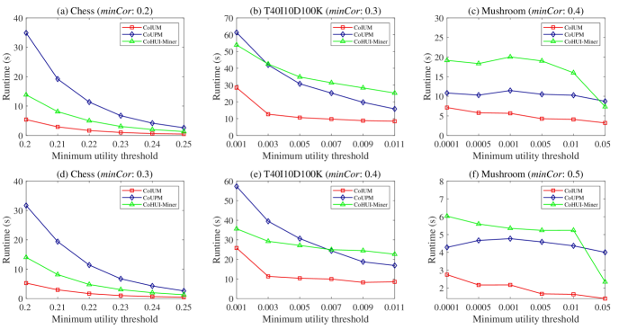
Figure 1: Runtime on dense datasets under changed minUtil.

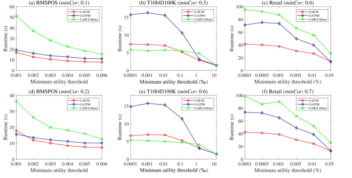
Figure 2: Runtime on sparse datasets under changed minUtil.

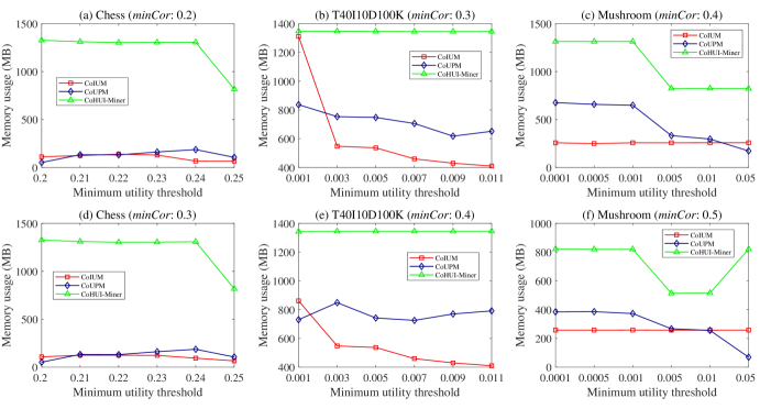
Figure 3: Memory on dense datasets under changed minUtil.

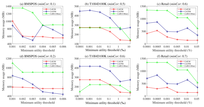
Figure 4: Memory on sparse datasets under changed minUtil.

5.2 Experiments on Runtime

We compare the runtime of CoIUM with two other algorithms: CoUPM and CoHUI-Miner. The runtime of all three algorithms on dense datasets with various minCor values was shown in Fig. 1. The results indicate that CoIUM is faster than CoUPM and CoHUI-Miner on all dense datasets. For example, on the Chess dataset with minCor = 0.2, the runtime of CoIUM is less than 5 seconds, while that of CoUPM is more than 10 seconds and that of CoHUI-Miner is about 8 seconds. On the T40I10D100K dataset with minCor = 0.3, the performance of CoIUM is 2X and 3X faster than that of CoUPM and CoHUI-Miner, respectively. On the Mushroom dataset with minCor = 0.4, the performance of CoIUM is 4X and 2X faster than that of CoHUI-Miner and CoUPM, respectively. We can see that the execution time of CoUPM and CoHUI-Miner increases dramatically as the utility of each dense dataset decreases to a certain point. On the contrary, when the utility of each dense dataset decreases to a certain extent, the execution time of CoIUM remains stable within a certain range.

The runtime of all three algorithms on sparse datasets with different minUtil and various minCor values was shown in Fig. 2. The results demonstrate that CoIUM is faster than CoUPM and CoHUI-Miner on BMSPOS (up to 1.2X and 2.3X, respectively) and Retail (up to 1.5X and 2X, respectively). On the T10I4D100K dataset, it is interesting that CoIUM has similar performance as CoHUI-Miner and the performance of CoIUM is 3X faster than that of CoUPM. The minCor threshold can also affect the efficiency of three algorithms, especially on dense datasets. For example, on the Mushroom dataset with minCor = 0.4, CoIUM takes about 5 seconds to complete the progress, while CoUPM requires 10 seconds and CoHUI-Miner requires 20 seconds. When minCor = 0.5, CoIUM takes about 2 seconds to complete the progress, whereas CoUPM requires 4 seconds and CoHUI-Miner requires 6 seconds. As can be seen, with the increase of minCor, the performance of the three algorithms also increases.

The most important reason why CoIUM is often faster than CoUPM and CoHUI-Miner is that CoIUM utilizes two effective upper bounds ($lu$ and $su$). Compared with the other two algorithms, $lu$ and $su$ can prune more space. Therefore, CoIUM only utilizes a few itemsets to discover HUIs. However, CoHUI-Miner has a large size of a projected dataset, which will produce more candidates, especially on dense datasets. CoUPM also takes a lot of time to construct the utility-list structure.

5.3 Experiments on Memory Usage

Memory consumption is an important indicator for evaluating the merits of data mining algorithms, so in this subsection, we will compare the memory usage between CoIUM, CoUPM, and CoHUI-Miner. Based on the same variable setting as shown in Fig. 1, the detailed results on the dense datasets are shown in Fig. 3. It can be clearly obtained that the memory consumption of CoIUM is much less than that of CoHUI-Miner on all dense datasets. For example, on the T40I10D100K dataset with minCor = 0.3, the memory loss of CoHUI-Miner is always maintained at about 1400 MB, while the memory usage of CoIUM is less than 1000 MB and remains below 500 MB. This result proves that the performance of CoIUM is much better than that of CoHUI-Miner, because CoHUI-Miner produces too many candidates and requires a lot of memory to store information. Then, on the Chess dataset, the memory usage of CoIUM is nearly the same but lower than CoUPM. However, the memory usage of CoIUM is often lower than that of CoUPM on T40I10D100K and Mushroom datasets. For instance, on the Mushroom dataset with minCor = 0.4, the memory usage of CoIUM tends to remain at 220 MB, while CoUPM remains between 200 MB and 600 MB. In most cases, the memory consumption of CoUPM exceeds 220 MB.

Based on the same variable setting as displayed in Fig. 2, the detailed results on the sparse datasets are shown in Fig. 4. As we can observe from the Retail dataset, the memory usage of CoIUM is much lower than that of both CoUPM and CoHUI-Miner (less than 2X and 3X, respectively). On the BMSPOS and T10I4D100K datasets, the memory usage of CoIUM is lower than that of CoHUI-Miner, and close to that of CoUPM when minUtil increases. Because of sparse datasets, the size of the transaction dataset is small, so both CoUPM and CoHUI-Miner require only a small amount of memory to conserve candidates.

The main reason why the memory consumption of CoIUM is lower than that of CoUPM in all datasets is that the projected technique can reduce dataset size more effectively than the utility-list used in the CoUPM algorithm. Although both CoIUM and CoHUI-Miner use the same projected technique, the consumption of CoIUM is lower than CoHUI-Miner on all datasets. The reason is that both of them use different strategies to explore CoHUIs. CoIUM uses two upper bounds ($lu$ and $su$) to reduce the number of candidates generated. These two upper bounds are more compact than TWU utilized in CoHUI-Miner, so they can remove more unpromising candidates than TWU. The number of candidates produced by CoIUM is lower than that of CoUPM and CoHUI-Miner. As a result, the memory consumption of CoIUM is lower than that of CoUPM and CoHUI-Miner.

Table 7: # Candidate generation under varying minUtil with fixed minCor

Dataset	minCor	# Algorithm	# candidate generation under different thresholds
			$\delta_{1}$	$\delta_{2}$	$\delta_{3}$	$\delta_{4}$	$\delta_{5}$	$\delta_{6}$
		#CoIUM	59,039	28,384	13,808	6,614	3,187	1,501
	0.2	#CoUPM	200,606	111,453	63,757	37,323	22,593	13,794
		#CoHUI-Miner	2620,117	1240,899	595,812	288,709	140,696	67,589
Chess		#CoIUM	59,039	28,384	13,808	6,614	3,187	1,501
	0.3	#CoUPM	200,606	111,453	63,757	37,323	22,593	13,794
		#CoHUI-Miner	2,620,117	1,240,899	595,812	288,709	140,696	67,589
		#CoIUM	152,930	15,935	3,738	1,475	957	796
	0.3	#CoUPM	447,807	140,222	69,670	35,506	21,179	13,068
		#CoHUI-Miner	17435,132	7761,519	3077,564	1362,147	863,037	626,828
T40I10D100K		#CoIUM	112,925	14,147	3,549	1,468	957	796
	0.4	#CoUPM	245,896	95,410	52,987	31,469	19,752	12,724
		#CoHUI-Miner	2449,760	1563,543	1107,732	823,317	673,769	585,371
		#CoIUM	276,518	269,858	253,590	97,812	88,277	45,928
	0.4	#CoUPM	281,139	277,600	267,469	105,995	96,669	57,134
		#CoHUI-Miner	13,045,179	12,697,922	12,367,803	4,615,310	4,083,339	2,015,229
Mushroom		#CoIUM	98,887	96,816	88,517	33,401	30,094	17,187
	0.5	#CoUPM	102,875	101,615	97,757	38,210	34,701	22,059
		#CoHUI-Miner	3,170,082	3,093,407	3,004,022	1,073,346	952,846	525,577
		#CoIUM	3,747,571	3,420,817	2,659,589	233,859	48,056	6,779
	0.6	#CoUPM	134,722,599	129,039,485	120,942,326	73,168,998	49,245,865	10,939,731
		#CoHUI-Miner	533,955,947	485,002,701	389,635,998	157,096,263	107,204,879	30,288,360
Retail		#CoIUM	3,615,594	3,297,971	2,570,798	231,801	47,899	6,773
	0.7	#CoUPM	134,588,149	128,906,771	120,821,509	73,158,370	49,245,259	10,939,665
		#CoHUI-Miner	311,399,670	292,452,873	264,220,651	154,067,657	106,915,555	30,200,504

5.4 Experiments on Candidates Generation

Table 7 shows the candidate generation results of CoIUM, CoUPM, and CoHUI-Miner, under different minUtil and minCor. Note that $\delta$ represents a different minUtil threshold, and its specific scope is from Fig. 1(a) to (c) and Fig. 2(a) to (c). The results indicate that the candidate generation by CoIUM is lower than CoUPM and CoHUI-Miner on dense datasets. For example, on T40I10D100K dataset with minCor = 0.3, the quantity of candidates increased by CoUPM is more than 2X higher than that of CoIUM, and the quantity of candidates generated by CoHUI-Miner is up to 10 orders of magnitude higher than that of CoIUM. With the increase of minUtil, the decrease of CoIUM is significantly greater than that of CoUPM and CoHUI-Miner. On the Mushroom dataset with minCor = 0.4, the quantity of candidates increased by CoIUM is always close to but lower than that of CoUPM, and the quantity of candidates produced by CoHUI-Miner is up to four orders of magnitude higher than that of CoIUM. These results prove that both CoUPM and CoHUI-Miner discover numerous meaningless Itemsets, which is why the runtime of CoIUM is better than CoUPM and CoHUI-Miner on all dense datasets. The reason why CoIUM generated fewer candidates than CoUPM and CoHUI-Miner on dense datasets is that the CoIUM algorithm adopts two tighter upper bounds (lu and su). These upper bounds can be used to remove more unpromising itemsets that do not satisfy the properties of CoHUIs.

On a spare dataset, it is found that the sum of candidates produced by CoIUM is also lower than that of CoUPM and CoHUI-Miner, especially on Retail dataset. For example, on Retail dataset with minCor = 0.6, the sum of candidates generated by CoUPM and CoHUI-Miner is up to 4 and 10 orders of magnitude higher than CoIUM respectively. And with the increase of minUtil, the gap between the number of candidates they produce becomes larger. With the increase of minCor on different datasets except Chess, the number of candidates generated by the three algorithms decreases correspondingly. It can be seen that minCor also has an impact on the discovery of HUIs. Because the data of Chess dataset is too dense, the small promotion of minCor cannot effectively filter out unpromising candidates.

5.5 Experiments on Scalability Test

Moreover, we test the scalability of CoIUM, CoUPM, and CoHUI-Miner. We adopt the size of the Retail dataset from 20% (= 17,632 transactions) to 100% (= 88,162 transactions) with minCor = 0.7. Fig. 5 shows the details of execution time and memory usage. From Fig. 5(a), We can know that the runtime of CoIUM, CoUPM, and CoHUI-Miner respectively increases linearly with the increasing dataset size. Compared with the other two algorithms, CoIUM has a smaller runtime increment because lu and su can reduce more unpromising candidates than that of TWU. At the same time, the gap in runtime between CoIUM and the other two algorithms is becoming larger. This conclusion proves that the pruning strategies of CoIUM are obviously better than those of the other two algorithms. In addition, we can see from Fig. 5(b) that with the growth of dataset size, the memory usage of CoIUM increases slowly and remains at about 100 MB, and the memory use of CoHUI-Miner also increases slowly and remains at about 1000 MB after a significant increase, while the memory use of CoUPM remains a decrease-increase-decrease phenomenon. We can see that with the increase in dataset size, the memory trend of CoIUM is more gentle than that of the other two algorithms. The results demonstrate that CoIUM has preferable scalability in runtime and memory consumption compared with CoUPM and CoHUI-Miner. In addition, the execution time and memory usage of CoIUM increase slowly when the data size increases. These results indicate that CoIUM is more suitable for large-scale datasets.

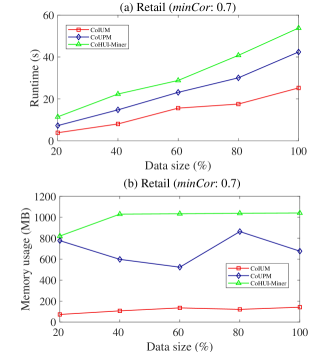
Figure 5: Runtime and memory scalability on Retail.

6 Conclusions

In this study, we present an efficient algorithm named CoIUM to extract the set of CoHUIs. The proposed CoIUM algorithm adopts two new upper bounds called local utility and subtree utility, which can prune more unpromising candidates effectively. Then, a novel array-based structure known as UA is applied to store useful information when pruning the search space. A novel technique called database projection is designed to reduce the cost of datasets in memory. In addition, we utilize TWU ascending order to sort all items. Extensive experiments on different datasets show that the performance of the CoIUM algorithm is obviously better than the CoUPM and CoHUI-Miner algorithms.

In the future, we would like to explore other novel data structures to reduce memory consumption effectively. We will extend the designed algorithm to different fields such as on-shelf utility mining, HUIM without setting minUtil and fuzzy utility mining. We also plan to apply the proposed algorithm to resolve other types of complex data (e.g., episodes, streaming data), not just static data.

References

- [1] P. Fournier-Viger, W. Gan, Y. Wu, M. Nouioua, W. Song, T. Truong, and H. Duong, “Pattern mining: Current challenges and opportunities,” in International Conference on Database Systems for Advanced Applications. Springer, 2022, pp. 34–49.
- [2] W. Gan, J. C. W. Lin, P. Fournier-Viger, H.-C. Chao, and P. S. Yu, “A survey of parallel sequential pattern mining,” ACM Transactions on Knowledge Discovery from Data, vol. 13, no. 3, pp. 1–34, 2019.
- [3] C. C. Aggarwal, M. A. Bhuiyan, and M. A. Hasan, “Frequent pattern mining algorithms: A survey,” in Frequent pattern mining, 2014, pp. 19–64.
- [4] C. J. Chu, V. S. Tseng, and T. Liang, “An efficient algorithm for mining temporal high utility itemsets from data streams,” Journal of Systems and Software, vol. 81, no. 7, pp. 1105–1117, 2008.
- [5] R. Agrawal, R. Srikant et al., “Fast algorithms for mining association rules,” in Proceedings of the 20th International Conference on Very Large Data Bases, vol. 1215, 1994, pp. 487–499.
- [6] J. Han, J. Pei, Y. Yin, and R. Mao, “Mining frequent patterns without candidate generation: A frequent-pattern tree approach,” Data Mining and Knowledge Discovery, vol. 8, no. 1, pp. 53–87, 2004.
- [7] J. M. Luna, P. Fournier-Viger, and S. Ventura, “Frequent itemset mining: A 25 years review,” Wiley Interdisciplinary Reviews: Data Mining and Knowledge Discovery, vol. 9, no. 6, p. e1329, 2019.
- [8] C. F. Ahmed, S. K. Tanbeer, B. S. Jeong, and Y. K. Lee, “Efficient tree structures for high utility pattern mining in incremental databases,” IEEE Transactions on Knowledge and Data Engineering, vol. 21, no. 12, pp. 1708–1721, 2009.
- [9] W. Gan, J. C.-W. Lin, P. Fournier-Viger, H.-C. Chao, V. S. Tseng, and P. S. Yu, “A survey of utility-oriented pattern mining,” IEEE Transactions on Knowledge and Data Engineering, vol. 33, no. 4, pp. 1306–1327, 2021.
- [10] M. Liu and J. Qu, “Mining high utility itemsets without candidate generation,” in Proceedings of the 21st ACM International Conference on Information and Knowledge Management, 2012, pp. 55–64.
- [11] Y. Liu, W. k. Liao, and A. Choudhary, “A two-phase algorithm for fast discovery of high utility itemsets,” in Proceedings of the Pacific-Asia Conference on Knowledge Discovery and Data Mining. Springer, 2005, pp. 689–695.
- [12] W. Gan, J. C. W. Lin, H. C. Chao, T. P. Hong, and P. S. Yu, “CoUPM: Correlated utility-based pattern mining,” in IEEE International Conference on Big Data, 2018, pp. 2607–2616.
- [13] V. S. Tseng, C. W. Wu, B. E. Shie, and P. S. Yu, “UP-Growth: an efficient algorithm for high utility itemset mining,” in Proceedings of the 16th ACM SIGKDD International Conference on Knowledge Discovery and Data Mining, 2010, pp. 253–262.
- [14] P. Fournier-Viger, C. W. Wu, S. Zida, and V. S. Tseng, “FHM: Faster high-utility itemset mining using estimated utility co-occurrence pruning,” in Proceedings of the International Symposium on Methodologies for Intelligent Systems, 2014, pp. 83–92.
- [15] S. Zida, P. Fournier-Viger, J. C. W. Lin, C. W. Wu, and V. S. Tseng, “EFIM: a fast and memory efficient algorithm for high-utility itemset mining,” Knowledge and Information Systems, vol. 51, no. 2, pp. 595–625, 2017.
- [16] L. T. Nguyen, P. Nguyen, T. D. Nguyen, B. Vo, P. Fournier-Viger, and V. S. Tseng, “Mining high-utility itemsets in dynamic profit databases,” Knowledge-Based Systems, vol. 175, pp. 130–144, 2019.
- [17] T. Wu, Y. Chen, and J. Han, “Re-examination of interestingness measures in pattern mining: a unified framework,” Data Mining and Knowledge Discovery, vol. 21, no. 3, pp. 371–397, 2010.
- [18] E. R. Omiecinski, “Alternative interest measures for mining associations in databases,” IEEE Transactions on Knowledge and Data Engineering, no. 1, pp. 57–69, 2003.
- [19] M. Barsky, S. Kim, T. Weninger, and J. Han, “Mining flipping correlations from large datasets with taxonomies,” bioinformatics, vol. 5, no. 4, pp. 370–381, 2011.
- [20] W. Gan, J. C. W. Lin, P. Fournier-Viger, H. C. Chao, and H. Fujita, “Extracting non-redundant correlated purchase behaviors by utility measure,” Knowledge-Based Systems, vol. 143, pp. 30–41, 2018.
- [21] R. Saeed, A. Rauf, F. H. Quradaa, and S. M. Asim, “Efficient utility tree-based algorithm to mine high utility patterns having strong correlation,” Complexity, vol. 2021, 2021.
- [22] B. Vo, L. V. Nguyen, V. V. Vu, M. T. Lam, T. T. Duong, L. T. Manh, T. T. Nguyen, L. T. Nguyen, and T. P. Hong, “Mining correlated high utility itemsets in one phase,” IEEE Access, vol. 8, pp. 90 465–90 477, 2020.
- [23] J. F. Qu, P. Fournier-Viger, M. Liu, B. Hang, and F. Wang, “Mining high utility itemsets using extended chain structure and utility machine,” Knowledge-Based Systems, vol. 208, p. 106457, 2020.
- [24] T. D. Nguyen, L. T. Nguyen, L. Vu, B. Vo, and W. Pedrycz, “Efficient algorithms for mining closed high utility itemsets in dynamic profit databases,” Expert Systems with Applications, vol. 186, p. 115741, 2021.
- [25] J. Liu, K. Wang, and B. C. Fung, “Direct discovery of high utility itemsets without candidate generation,” in Proceedings of the IEEE 12th International Conference on Data Mining, 2012, pp. 984–989.
- [26] H. Ryang and U. Yun, “Indexed list-based high utility pattern mining with utility upper-bound reduction and pattern combination techniques,” Knowledge and Information Systems, vol. 51, no. 2, pp. 627–659, 2017.
- [27] Q. H. Duong, P. Fournier-Viger, H. Ramampiaro, K. Nørvåg, and T. L. Dam, “Efficient high utility itemset mining using buffered utility-lists,” Applied Intelligence, vol. 48, no. 7, pp. 1859–1877, 2018.
- [28] J. C. W. Lin, P. Fournier-Viger, and W. Gan, “FHN: An efficient algorithm for mining high-utility itemsets with negative unit profits,” Knowledge-Based Systems, vol. 111, pp. 283–298, 2016.
- [29] W. Gan, S. Wan, J. Chen, C. M. Chen, and L. Qiu, “TopHUI: Top- high-utility itemset mining with negative utility,” in Proceedings of the IEEE International Conference on Big Data, 2020, pp. 5350–5359.
- [30] J. Chen, X. Guo, W. Gan, C. M. Chen, W. Ding, and G. Chen, “On-shelf utility mining from transaction database,” Engineering Applications of Artificial Intelligence, vol. 107, p. 104516, 2022.
- [31] W. Song, L. Liu, and C. Huang, “Generalized maximal utility for mining high average-utility itemsets,” Knowledge and Information Systems, vol. 63, no. 11, pp. 2947–2967, 2021.
- [32] S. Wan, J. Chen, P. Zhang, W. Gan, and T. Gu, “Discovering top- profitable patterns for smart manufacturing,” in Companion Proceedings of the Web Conference, 2022, pp. 1–9.
- [33] T. Mai, B. Vo, and L. T. Nguyen, “A lattice-based approach for mining high utility association rules,” Information Sciences, vol. 399, pp. 81–97, 2017.
- [34] S. Wan, W. Gan, X. Guo, J. Chen, and U. Yun, “FUIM: Fuzzy utility itemset mining,” arXiv preprint, arXiv:2111.00307, 2021.
- [35] J. Miao, S. Wan, W. Gan, J. Sun, and J. Chen, “Targeted high-utility itemset querying,” IEEE Transactions on Artificial Intelligence, DOI: 10.1109/TAI.2022.3171530, 2022.
- [36] X. Han, X. Liu, J. Li, and H. Gao, “Efficient top- high utility itemset mining on massive data,” Information Sciences, vol. 557, pp. 382–406, 2021.
- [37] Y. Baek, U. Yun, H. Kim, J. Kim, B. Vo, T. Truong, and Z.-H. Deng, “Approximate high utility itemset mining in noisy environments,” Knowledge-Based Systems, vol. 212, p. 106596, 2021.
- [38] W. Song, C. Fang, and W. Gan, “TopUMS: Top- utility mining in stream data,” in The International Conference on Data Mining Workshops. IEEE, 2021, pp. 615–622.
- [39] U. Yun, “Efficient mining of weighted interesting patterns with a strong weight and/or support affinity,” Information Sciences, vol. 177, no. 17, pp. 3477–3499, 2007.
- [40] C. F. Ahmed, S. K. Tanbeer, B. S. Jeong, and H. J. Choi, “A framework for mining interesting high utility patterns with a strong frequency affinity,” Information Sciences, vol. 181, no. 21, pp. 4878–4894, 2011.
- [41] J. C. W. Lin, W. Gan, P. Fournier-Viger, T. P. Hong, and H. C. Chao, “FDHUP: Fast algorithm for mining discriminative high utility patterns,” Knowledge and Information Systems, vol. 51, no. 3, pp. 873–909, 2017.
- [42] P. Fournier-Viger, Y. Zhang, J. C. W. Lin, D. T. Dinh, and H. Bac Le, “Mining correlated high-utility itemsets using various measures,” Logic Journal of the IGPL, vol. 28, no. 1, pp. 19–32, 2020.
- [43] R. Rymon, “Search through systematic set enumeration,” in Proceedings of the 3rd International Conference on Principles of Knowledge Representation and Reasoning, 1992, pp. 539–550.