Testing Upward Planarity of Partial $2$-Trees

Abstract

We present an $O(n^{2})$-time algorithm to test whether an $n$-vertex directed partial $2$-tree is upward planar. This result improves upon the previously best known algorithm, which runs in $O(n^{4})$ time.

1 Introduction

A digraph is upward planar if it admits a drawing that is at the same time planar, i.e., it has no crossings, and upward, i.e., all edges are drawn as curves monotonically increasing in the vertical direction. Upward planarity is a natural variant of planarity for directed graphs and finds applications in those domains where one wants to visualize networks with a hierarchical structure.

Upward planarity is a classical research topic in Graph Drawing since the early 90s. Garg and Tamassia have shown that recognizing upward planar digraphs is $\mathrm{NP}$-complete [13], however polynomial-time algorithms have been proposed for various cases, including digraphs with fixed embedding [1], single-source digraphs [2, 3, 16, 17], outerplanar digraphs [18]. The case of directed partial $2$-trees, which is of central interest to this paper and includes, among others, series-parallel digraphs, has been investigated by Didimo et al. [10] who presented an $\mathcal{O}(n^{4})$-time testing algorithm. The parameterized complexity of the upward planarity testing problem has also been investigated [4, 5, 10, 15].

In this paper, we present an $\mathcal{O}(n^{2})$-time algorithm to test upward planarity of directed partial $2$-trees, improving upon the $\mathcal{O}(n^{4})$-time algorithm by Didimo et al. [10]. There are two main ingredients that allow us to achieve such result.

First, following the approach in [5], our algorithm traverses the SPQ-tree of the input digraph $G$ while computing, for each component of $G$, the possible “shapes” of its upward planar embeddings. The algorithm in [5] only works for expanded digraphs, i.e., digraphs such that every vertex has at most one incoming or outgoing edge. Although every digraph can be made expanded while preserving its upward planarity by “splitting” its vertices [2], this modification might not maintain that the digraph is a directed partial $2$-tree; see Fig. 1. We present a novel algorithm that is applicable to non-expanded digraphs. We propose a new strategy to process P-nodes, which is simpler than the one of [5] and allows us to compute some additional information that is needed by the second ingredient. Further, we give a more efficient procedure than the one of [5] to process the S-nodes; this is vital for the overall running time of our algorithm.

Figure 1: Splitting a vertex in a non-expanded directed partial $2$-tree (a) might result in an expanded digraph (b) which is not a directed partial $2$-tree.

Second, the traversal of the SPQ-tree $T$ of $G$ tests the upward planarity of $G$ with the constraint that the edge corresponding to the root of $T$ is incident to the outer face. Then $\mathcal{O}(n)$ traversals with different choices for the root of $T$ can be used to test the upward planarity of $G$ without that constraint. However, following a recently developed strategy [11, 12], in the first traversal of $T$ we compute some information additional to the possible shapes of the upward planar embeddings of the components of $G$. A clever use of this information allows us to handle P-nodes more efficiently in later traversals. Our testing algorithms can be enhanced to output an upward planar drawing, if one exists, although we do not describe the process explicitly.

Paper organization

In Section 2 we give some preliminaries. In Section 3 we describe the algorithm for biconnected digraphs with a prescribed edge on the outer face, while in Section 4 we deal with general biconnected digraphs. Section 5 extends our result to simply connected digraphs. Future research directions are presented in Section 6. Lemmas and theorems whose proofs are omitted are marked with a $(\star)$ and can be found in the full version of the paper.

2 Preliminaries

In a digraph, a switch is a source or a sink. The underlying graph of a digraph is the undirected graph obtained by ignoring the edge directions. When we mention connectivity of a digraph, we mean the connectivity of its underlying graph.

A planar embedding of a connected graph is an equivalence class of planar drawings, where two drawings are equivalent if: (i) the clockwise order of the edges incident to each vertex is the same; and (ii) the sequence of vertices and edges along the boundary of the outer face is the same.

A drawing of a digraph is upward if every edge is represented by a Jordan arc whose $y$-coordinates monotonically increase from the source to the sink of the edge. A drawing of a digraph is upward planar if it is both upward and planar. An upward planar drawing of a graph determines an assignment of labels to the angles of the corresponding planar embedding, where an angle $\alpha$ at a vertex $u$ in a face $f$ of a planar embedding represents an incidence of $u$ on $f$. Specifically, $\alpha$ is flat and gets label $0$ if the edges delimiting it are one incoming and one outgoing at $u$. Otherwise, $\alpha$ is a switch angle; in this case, $\alpha$ is small (and gets label $-1$) or large (and gets label $1$) depending on whether the (geometric) angle at $f$ representing $\alpha$ is smaller or larger than $180^{\circ}$, respectively, see Fig. 2. An upward planar embedding is an equivalence class of upward planar drawings of a digraph $G$, where two drawings are equivalent if they determine the same planar embedding $\mathcal{E}$ for $G$ and the same label assignment for the angles of $\mathcal{E}$.

Figure 2: (a) Labels at the angles of an upward planar embedding $\mathcal{E}$ of a biconnected directed partial $2$-tree $G$; the missing labels are $-1$. (b) An SPQ-tree $T$ of $G$ with respect to $e^{*}$. The restriction of $\mathcal{E}$ to $G_{\sigma^{*}}$ is a $uv$-external upward planar embedding $\mathcal{E}_{\sigma^{*}}$ with shape description $\langle 0,\allowbreak 1,\allowbreak 1,\allowbreak 0,\allowbreak\texttt{out},\allowbreak\texttt{out},\allowbreak\texttt{in},\allowbreak\texttt{out}\rangle$. The shape sequence of $\mathcal{E}_{\sigma^{*}}$ is $[\langle 0,\allowbreak 0,\allowbreak 1,\allowbreak 1,\allowbreak\texttt{out},\allowbreak\texttt{out},\allowbreak\texttt{in},\allowbreak\texttt{in}\rangle,\langle 0,\allowbreak 0,\allowbreak 1,\allowbreak 1,\allowbreak\texttt{out},\allowbreak\texttt{out},\allowbreak\texttt{in},\allowbreak\texttt{in}\rangle,\langle-1,\allowbreak 1,\allowbreak 1,\allowbreak 1,\allowbreak\texttt{out},\allowbreak\texttt{out},\allowbreak\texttt{out},\allowbreak\texttt{out}\rangle,\langle-1,\allowbreak 1,\allowbreak 1,\allowbreak 1,\allowbreak\texttt{out},\allowbreak\texttt{out},\allowbreak\texttt{out},\allowbreak\texttt{out}\rangle]$. The contracted shape sequence of $\mathcal{E}_{\sigma^{*}}$ is $[\langle 0,\allowbreak 0,\allowbreak 1,\allowbreak 1,\allowbreak\texttt{out},\allowbreak\texttt{out},\allowbreak\texttt{in},\allowbreak\texttt{in}\rangle,\langle-1,\allowbreak 1,\allowbreak 1,\allowbreak 1,\allowbreak\texttt{out},\allowbreak\texttt{out},\allowbreak\texttt{out},\allowbreak\texttt{out}\rangle]$.

Theorem 2.1 ([1, 10])

Let $G$ be a digraph with planar embedding $\mathcal{E}$, and $\lambda$ be a label assignment for the angles of $\mathcal{E}$. Then $\mathcal{E}$ and $\lambda$ define an upward planar embedding of $G$ if and only if the following hold:

1. (UP0) If $\alpha$ is a switch angle then $\alpha$ is small or large, otherwise it is flat.

2. (UP1) If $v$ is a switch vertex, the number of small, flat and large angles incident to $v$ is equal to $\deg(v)-1$, $0$, and $1$, respectively.

3. (UP2) If $v$ is a non-switch vertex, the number of small, flat and large angles incident to $v$ is equal to $\deg(v)-2$, $2$, and $0$, respectively.

4. (UP3) If $f$ is an internal face (the outer face) of $\mathcal{E}$, the number of small angles in $f$ is equal to the number of large angles in $f$ plus $2$ (resp. minus $2$).

The class of partial $2$-trees can be defined equivalently as the graphs with treewidth at most two, or as the graphs that exclude $K_{4}$ as a minor, or as the subgraphs of the $2$-trees. Notably, it includes the class of series-parallel graphs.

Let $G$ be a biconnected partial $2$-tree and let $e^{*}$ be an edge of $G$. An SPQ-tree $T$ of $G$ with respect to $e^{*}$ (see Fig. 2) is a tree that describes a recursive decomposition of $G$ into its “components”. SPQ-trees are a specialization of SPQR-trees [8, 14]. Each node $\mu$ of $T$ represents a subgraph $G_{\mu}$ of $G$, called the pertinent graph of $\mu$, and is associated with two special vertices of $G_{\mu}$, called poles of $\mu$. The nodes of $T$ are of three types: a Q-node $\mu$ represents an edge whose end-vertices are the poles of $\mu$, an S-node $\mu$ with children $\nu_{1}$ and $\nu_{2}$ represents a series composition in which the components $G_{\nu_{1}}$ and $G_{\nu_{2}}$ share a pole to form $G_{\mu}$, and a P-node $\mu$ with children $\nu_{1},\dots,\nu_{k}$ represents a parallel composition in which the components $G_{\nu_{1}},\dots,G_{\nu_{k}}$ share both poles to form $G_{\mu}$. The root of $T$ is the Q-node representing the edge $e^{*}$. By our definition, every S-node has exactly two children that can also be S-nodes; because of this assumption, the SPQ-tree of a biconnected partial $2$-tree is not unique. However, from an SPQ-tree $T$, we can obtain an SPQ-tree of $G$ with respect to another reference edge $e^{**}$ by selecting the Q-node representing $e^{**}$ as the new root of $T$ (see Fig. 3).

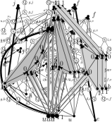
Figure 3: Two different choices for the root of the SPQ-tree of Fig. 2. The reference edge is shown in bold.

A directed partial $2$-tree is a digraph whose underlying graph is a partial $2$-tree. When talking about an SPQ-tree $T$ of a biconnected directed partial $2$-tree $G$, we always refer to an SPQ-tree of its underlying graph, although the edges of the pertinent graph of each node of $T$ are oriented as in $G$. Let $\mu$ be a node of $T$ with poles $u$ and $v$. A $uv$-external upward planar embedding of $G_{\mu}$ is an upward planar embedding of $G_{\mu}$ in which $u$ and $v$ are incident to the outer face. In our algorithms, when testing the upward planarity of $G$, choosing an edge $e^{*}$ of $G$ as the root of $T$ corresponds to requiring $e^{*}$ to be incident to the outer face of the sought upward planar embedding $\mathcal{E}$ of $G$. For each node $\mu$ of $T$ with poles $u$ and $v$, the restriction of $\mathcal{E}$ to $G_{\mu}$ is a $uv$-external upward planar embedding $\mathcal{E}_{\mu}$ of $G_{\mu}$. In [5], the possible “shapes” of the cycle bounding the outer face $f_{\mu}$ of $\mathcal{E}_{\mu}$ have been described by the concept of shape description. This is the tuple $\langle\tau_{l},\allowbreak\tau_{r},\allowbreak\lambda(u),\allowbreak\lambda(v),\allowbreak\rho^{l}_{u},\allowbreak\rho^{r}_{u},\allowbreak\rho^{l}_{v},\allowbreak\rho^{r}_{v}\rangle$, defined as follows. Let the left outer path $P_{l}$ (the right outer path $P_{r}$) of $\mathcal{E}_{\mu}$ be the path that is traversed when walking from $u$ to $v$ in clockwise (resp. counterclockwise) direction along the boundary of $f_{\mu}$. The value $\tau_{l}$, called left-turn-number of $\mathcal{E}_{\mu}$, is the sum of the labels of the angles at the vertices of $P_{l}$ different from $u$ and $v$ in $f_{\mu}$; the right-turn-number $\tau_{r}$ of $\mathcal{E}_{\mu}$ is defined similarly. The values $\lambda(u)$ and $\lambda(v)$ are the labels of the angles at $u$ and $v$ in $f_{\mu}$, respectively. The value $\rho^{l}_{u}$ is in (out) if the edge incident to $u$ in $P_{l}$ is incoming (outgoing) at $u$; the values $\rho^{r}_{u}$, $\rho^{l}_{v}$, and $\rho^{r}_{v}$ are defined similarly. The values of a shape description depend on each other, as in the following.

[[5]] The shape description $\langle\tau_{l},\allowbreak\tau_{r},\allowbreak\lambda(u),\allowbreak\lambda(v),\allowbreak\rho^{l}_{u},\allowbreak\rho^{r}_{u},\allowbreak\rho^{l}_{v},\allowbreak\rho^{r}_{v}\rangle$ of $\mathcal{E}_{\mu}$ satisfies the following properties:

1. $\rho^{l}_{u}$ and $\rho^{r}_{u}$ have the same value if $\lambda(u)\in\{-1,1\}$, while they have different values if $\lambda(u)=0$;

2. $\rho^{l}_{v}$ and $\rho^{r}_{v}$ have the same value if $\lambda(v)\in\{-1,1\}$, while they have different values if $\lambda(v)=0$;

3. $\rho^{l}_{u}$ and $\rho^{l}_{v}$ have the same value if $\tau_{l}$ is odd, while they have different values if $\tau_{l}$ is even;

4. $\tau_{l}+\tau_{r}+\lambda(u)+\lambda(v)=2$.

A set $\mathcal{S}$ of shape descriptions is $n$-universal if, for every $n$-vertex biconnected directed partial $2$-tree $G$, for every rooted SPQ-tree $T$ of $G$, for every node $\mu$ of $T$ with poles $u$ and $v$, and for every $uv$-external upward planar embedding $\mathcal{E}_{\mu}$ of $G_{\mu}$, the shape description of $\mathcal{E}_{\mu}$ belongs to $\mathcal{S}$. Thus, an $n$-universal set is a super-set of the feasible set $\mathcal{F}_{\mu}$ of $\mu$, that is, the set of shape descriptions $s$ such that $G_{\mu}$ admits a $uv$-external upward planar embedding with shape description $s$. Our algorithm will determine $\mathcal{F}_{\mu}$ by inspecting each shape description $s$ in an $n$-universal set and deciding whether $G_{\mu}$ admits a $uv$-external upward planar embedding with shape description $s$ or not. We have the following lemmas.

Lemma 1 ($\star$)

An $n$-universal set $\mathcal{S}$ of shape descriptions with $|\mathcal{S}|\in\mathcal{O}(n)$ can be constructed in $\mathcal{O}(n)$ time.

Lemma 2 ($\star$)

Any subset $\mathcal{F}$ of an $n$-universal set can be stored in $\mathcal{O}(n)$ time and space and querying whether a shape description is in $\mathcal{F}$ takes $\mathcal{O}(1)$ time.

Consider a P-node $\mu$ in an SPQ-tree $T$ of a biconnected directed partial $2$-tree $G$. Let $\nu_{1},\dots,\nu_{k}$ be the children of $\mu$ in $T$. Consider any $uv$-external upward planar embedding $\mathcal{E}_{\mu}$ of $G_{\mu}$. For $i=1,\dots,k$, the restriction of $\mathcal{E}_{\mu}$ to $G_{\nu_{i}}$ is a $uv$-external upward planar embedding $\mathcal{E}_{\nu_{i}}$ of $G_{\nu_{i}}$; let $\sigma_{i}$ be the shape description of $\mathcal{E}_{\nu_{i}}$. Assume that $\mathcal{E}_{\nu_{1}},\dots,\mathcal{E}_{\nu_{k}}$ appear in this clockwise order around $u$, where the left outer path of $\mathcal{E}_{\nu_{1}}$ and the right outer path of $\mathcal{E}_{\nu_{k}}$ delimit the outer face of $\mathcal{E}_{\mu}$. We call $\sigma=[\sigma_{1},\dots,\sigma_{k}]$ the shape sequence of $\mathcal{E}_{\mu}$. Further, consider the sequence $S=[s_{1},\dots,s_{x}]$ obtained from $\sigma$ by identifying consecutive identical shape descriptions. We call $S$ the contracted shape sequence of $\mathcal{E}_{\mu}$; see Fig. 2.

3 A Prescribed Edge on the Outer Face

Let $G$ be an $n$-vertex biconnected directed partial $2$-tree and $T$ be its SPQ-tree rooted at any Q-node $\rho^{*}$, which corresponds to an edge $e^{*}$ of $G$. In this section, we show an algorithm that computes the feasible set $\mathcal{F}_{\mu}$ of every node $\mu$ of $T$. Let $u$ and $v$ be the poles of $\mu$. Note that $G$ admits an upward planar embedding such that $e^{*}$ is incident to the outer face if and only if the feasible set of $\rho^{*}$ is non-empty. Hence, the algorithm could be applied repeatedly (once for each Q-node as the root) to test the upward planarity of $G$; however, in Section 4 we devise a more efficient way to handle multiple choices for the root of $T$. We first deal with S-nodes, then with P-nodes, and finally with the root of $T$. For Q-nodes, it is easy to show the following lemma.

Lemma 3 ([5])

For a non-root Q-node $\mu$, $\mathcal{F}_{\mu}$ can be computed in $\mathcal{O}(1)$ time.

S-nodes. We improve an algorithm from [5]. Let $\nu_{1}$ and $\nu_{2}$ be the children of $\mu$ in $T$, let $n^{\mu}_{1}=|V(G_{\nu_{1}})|$ and $n^{\mu}_{2}=|V(G_{\nu_{2}})|$, and let $w$ be the vertex shared by $G_{\nu_{1}}$ and $G_{\nu_{2}}$. Furthermore, let $n^{\mu}_{3}$ be the number of vertices in the subgraph $H_{\mu}$ of $G$ induced by $V(G)\setminus V(G_{\mu})\cup\{u,v\}$. Note that $n^{\mu}_{3}=|V(G)|-(n^{\mu}_{1}+n^{\mu}_{2})+3$. We distinguish two cases, depending on which of $n^{\mu}_{1}$, $n^{\mu}_{2}$, and $n^{\mu}_{3}$ is largest.

If $n^{\mu}_{3}\geq\max(n^{\mu}_{1},n^{\mu}_{2})$, we proceed as in [5, Lemma 6], by combining every shape description in $\mathcal{F}_{\nu_{1}}$ with every shape description in $\mathcal{F}_{\nu_{2}}$; for every such combination, the algorithm assigns the angles at $w$ in the outer face with every possible label in $\{-1,0,1\}$. If the combination and assignment result in a shape description $s$ of $\mu$ (the satisfaction of the properties of Theorem 2.1 are checked here), the algorithm adds $s$ to $\mathcal{F}_{\mu}$. This allows us to compute the feasible set $\mathcal{F}_{\mu}$ of $\mu$ in time $\mathcal{O}(n+|\mathcal{F}_{\nu_{1}}|\cdot|\mathcal{F}_{\nu_{2}}|)$, which is in $\mathcal{O}(n+n^{\mu}_{1}\cdot n^{\mu}_{2})$, as $|\mathcal{F}_{\nu_{1}}|\in\mathcal{O}(n^{\mu}_{1})$ and $|\mathcal{F}_{\nu_{2}}|\in\mathcal{O}(n^{\mu}_{2})$ by Lemma 1.

The most interesting case is when, say, $n^{\mu}_{1}\geq\max(n^{\mu}_{2},n^{\mu}_{3})$. Here, in order to keep the overall runtime in $\mathcal{O}(n^{2})$, we cannot combine every shape description in $\mathcal{F}_{\nu_{1}}$ with every shape description in $\mathcal{F}_{\nu_{2}}$. Rather, we proceed as follows. Note that every shape description in $\mathcal{F}_{\mu}$ whose absolute value of the (left- or right-) turn-number exceeds $n^{\mu}_{3}+4$ does not result in an upward planar embedding of $G$, by Property UP3 of Theorem 2.1 and since the absolute value of the turn-number of any path in any upward planar embedding of $H_{\mu}$ does not exceed $n^{\mu}_{3}$. We hence construct an $(n^{\mu}_{3}+4)$-universal set $\mathcal{S}$ in $\mathcal{O}(n^{\mu}_{3})$ time by Lemma 1, and then test whether each shape description $s$ in $\mathcal{S}$ belongs to the feasible set $\mathcal{F}_{\mu}$ of $\mu$. In order to do that, we consider every shape description $s_{2}$ in $\mathcal{F}_{\nu_{2}}$ individually. There are $\mathcal{O}(1)$ shape descriptions in $\mathcal{F}_{\nu_{1}}$ which combined with $s_{2}$ might result in $s$, since the turn numbers add to each other when combining the shape descriptions in $\mathcal{F}_{\nu_{1}}$ and $\mathcal{F}_{\nu_{2}}$, with a constant offset. Hence, by Lemma 2, we check in $\mathcal{O}(1)$ time if there is a shape description $s_{1}$ in $\mathcal{F}_{\nu_{1}}$ which combined with $s_{2}$ leads to $s$. The running time of this procedure is hence $\mathcal{O}(n+n^{\mu}_{2}\cdot n^{\mu}_{3})$, as $|\mathcal{F}_{\nu_{2}}|\in\mathcal{O}(n^{\mu}_{2})$ and $|\mathcal{S}|\in\mathcal{O}(n^{\mu}_{3})$ by Lemma 1. This yields the following.

Lemma 4

Let $\mu$ be an S-node of $T$ with children $\nu_{1}$ and $\nu_{2}$. Given the feasible sets $\mathcal{F}_{\nu_{1}}$ and $\mathcal{F}_{\nu_{2}}$ of $\nu_{1}$ and $\nu_{2}$, respectively, the feasible set $\mathcal{F}_{\mu}$ of $\mu$ can be computed in $\mathcal{O}(n+\min\{n^{\mu}_{1}\cdot n^{\mu}_{2},~{}n^{\mu}_{2}\cdot n^{\mu}_{3},~{}n^{\mu}_{1}\cdot n^{\mu}_{3}\})$ time.

P-nodes. To compute the feasible set $\mathcal{F}_{\mu}$ of a P-node $\mu$ from the feasible sets $\mathcal{F}_{\nu_{1}},\dots,\mathcal{F}_{\nu_{k}}$ of its children, the algorithm constructs an $n$-universal set $\mathcal{S}$ in $\mathcal{O}(n)$ time by Lemma 1. Then it examines every shape description $s\in\mathcal{S}$ and decides whether it belongs to $\mathcal{F}_{\mu}$. Hence, we focus on a single shape description $s$ and give an algorithm that decides in $\mathcal{O}(k)$ time whether $s$ belongs to $\mathcal{F}_{\mu}$.

The basic structural tool we need for our algorithm is the following lemma. We call generating set $\mathcal{G}(s)$ of a shape description $s$ the set of contracted shape sequences that the pertinent graph of any P-node with poles $u$ and $v$ can have in a $uv$-external upward planar embedding with shape description $s$.

Lemma 5 ($\star$)

For any shape description $s$, $\mathcal{G}(s)$ has size $\mathcal{O}(1)$ and can be constructed in $\mathcal{O}(1)$ time. Also, any sequence in $\mathcal{G}(s)$ has $\mathcal{O}(1)$ length.

A contracted shape sequence $S\in\mathcal{G}(s)$ is realizable by $\mu$ if there exists a $uv$-external upward planar embedding of $G_{\mu}$ whose contracted shape sequence is a subsequence of $S$ containing the first and last elements of $S$.

We now describe an algorithm that decides in $O(k)$ time whether $s$ belongs to $\mathcal{F}_{\mu}$. Also, for each contracted shape sequence $S=[s_{1},\dots,s_{x}]$ in the generating set $\mathcal{G}(s)$ of $s$, the algorithm computes and stores the following information:

• Three labels $\textsc{f}_{1}(\mu,S)$, $\textsc{f}_{2}(\mu,S)$, and $\textsc{f}_{3}(\mu,S)$ which reference three distinct children $\nu_{i}$ of $\mu$ such that $s_{1}\in\mathcal{F}_{\nu_{i}}$.

• Three labels $\textsc{l}_{1}(\mu,S)$, $\textsc{l}_{2}(\mu,S)$, and $\textsc{l}_{3}(\mu,S)$ which reference three distinct children $\nu_{i}$ of $\mu$ such that $s_{x}\in\mathcal{F}_{\nu_{i}}$.

• Two labels $\textsc{uf}_{1}(\mu,S)$ and $\textsc{uf}_{2}(\mu,S)$ which reference two distinct children $\nu_{i}$ of $\mu$ such that $\mathcal{F}_{\nu_{i}}$ does not contain any shape description in $S$.

For each label type, if the number of children with the described properties is smaller than the number of labels, then labels with larger indices are null. We call the set of relevant labels for $\mu$ and $S$ the set of labels described above.

The algorithm is as follows. First, by Lemma 5, we construct $\mathcal{G}(s)$ in $\mathcal{O}(1)$ time. Then we consider each sequence $S=[s_{1},\dots,s_{x}]$ in $\mathcal{G}(s)$. By Lemma 5, there are $\mathcal{O}(1)$ such sequences, each with length $\mathcal{O}(1)$. We decide whether $S$ is realizable by $\mu$ and compute the set of relevant labels for $\mu$ and $S$ as follows.

We initialize all the labels to null and process $\nu_{1},\dots,\nu_{k}$ one by one. For each $\nu_{i}$, by Lemma 2 we test in $\mathcal{O}(1)$ time which of the shape descriptions $s_{1},\dots,s_{x}$ belong to $\mathcal{F}_{\nu_{i}}$ and update the labels accordingly. For example, if $s_{1}\in\mathcal{F}_{\nu_{i}}$, then we update $\textsc{f}_{j}(\mu,S)=\nu_{i}$ for the smallest $j\in\{1,2,3\}$ with $\textsc{f}_{j}(\mu,S)=\textsc{null}$.

After processing $\nu_{1},\dots,\nu_{k}$, we decide whether $S$ is realizable by $\mu$ as follows. If $\textsc{uf}_{1}(\mu,S)\neq\textsc{null}$, then $S$ is not realizable by $\mu$. Otherwise, each feasible set $\mathcal{F}_{\nu_{i}}$ contains a shape description among $s_{1},\dots,s_{x}$. Still, we have to check whether $\mathcal{F}_{\nu_{i}}$ contains $s_{1}$ and $\mathcal{F}_{\nu_{j}}$ contains $s_{x}$, for two distinct nodes $\nu_{i}$ and $\nu_{j}$. If $\textsc{f}_{1}(\mu,S)=\textsc{null}$ or $\textsc{l}_{1}(\mu,S)=\textsc{null}$, then $S$ is not realizable by $\mu$, as the feasible set of no child contains $s_{1}$ or $s_{x}$, respectively. Otherwise, if $\textsc{f}_{1}(\mu,S)\neq\textsc{l}_{1}(\mu,S)$, then $S$ is realizable by $\mu$, as $\textsc{f}_{1}(\mu,S)$ can be assigned with $s_{1}$ and $\textsc{l}_{1}(\mu,S)$ with $s_{x}$. Otherwise, if $\textsc{f}_{2}(\mu,S)\neq\textsc{null}$ or $\textsc{l}_{2}(\mu,S)\neq\textsc{null}$, then $S$ is realizable by $\mu$, as $\textsc{f}_{2}(\mu,S)$ can be assigned with $s_{1}$ and $\textsc{l}_{1}(\mu,S)$ with $s_{x}$, or $\textsc{f}_{1}(\mu,S)$ can be assigned with $s_{1}$ and $\textsc{l}_{2}(\mu,S)$ with $s_{x}$, respectively. Otherwise, $S$ is not realizable by $\mu$, as $s_{1}$ and $s_{x}$ are in the feasible set of a single child $\textsc{f}_{1}(\mu,S)=\textsc{l}_{1}(\mu,S)$ of $\mu$.

Finally, we have that $s$ belongs to $\mathcal{F}_{\mu}$ if and only if there exists a contracted shape sequence $S$ in the generating set $\mathcal{G}(s)$ of $s$ which is realizable by $\mu$.

Lemma 6 ($\star$)

Let $\mu$ be an P-node of $T$ with children $\nu_{1},\dots,\nu_{k}$. Given their feasible sets $\mathcal{F}_{\nu_{1}},\dots,\mathcal{F}_{\nu_{k}}$, the feasible set $\mathcal{F}_{\mu}$ of $\mu$ can be computed in $\mathcal{O}(nk)$ time. Further, for every shape description $s$ in an $n$-universal set $\mathcal{S}$ and every contracted shape sequence $S$ in the generating set $\mathcal{G}(s)$ of $s$, the set of relevant labels for $\mu$ and $S$ can be computed and stored in overall $\mathcal{O}(nk)$ time and space.

Root. As in [5], the root $\rho^{*}$ of $T$ is treated as a P-node with two children, whose pertinent graphs are $e^{*}$ and the pertinent graph of the child $\sigma^{*}$ of $\rho^{*}$ in $T$.

Lemma 7 ([5])

Given the feasible set $\mathcal{F}_{\sigma^{*}}$, the feasible set $\mathcal{F}_{\rho^{*}}$ of the root $\rho^{*}$ of $T$ can be computed in $\mathcal{O}(n)$ time.

4 No Prescribed Edge on the Outer Face

In this section, we show an $\mathcal{O}(n^{2})$-time algorithm to test the upward planarity of a biconnected directed partial $2$-tree $G$. Let $e_{1},\dots,e_{m}$ be any order of the edges of $G$. For $i=1,\dots,m$, let $\rho_{i}$ be the Q-node of the SPQ-tree $T$ of $G$ corresponding to $e_{i}$ and $T_{i}$ be the rooted tree obtained by selecting $\rho_{i}$ as the root of $T$. For a node $\mu$ of $T$, distinct choices for the root of $T$ define different pertinent graphs $G_{\mu}$ of $\mu$. Thus, we change the previous notation and denote by $G_{\mu\rightarrow\tau}$ and $\mathcal{F}_{\mu\rightarrow\tau}$ the pertinent graph and the feasible set of a node $\mu$ when its parent is a node $\tau$. We denote by $\mathcal{F}_{\rho_{i}}$ the feasible set of the root $\rho_{i}$ of $T_{i}$.

Our algorithm performs traversals of $T_{1},\dots,T_{m}$. The traversal of $T_{1}$ is special; it is a bottom-up traversal using the results from Section 3 to compute the feasible set $\mathcal{F}_{\mu\rightarrow\tau}$ of every node $\mu$ with parent $\tau$ in $T_{1}$, as well as auxiliary information that is going to be used by later traversals. For $i=2,\dots,m$, we perform a top-down traversal of $T_{i}$ that computes the feasible set $\mathcal{F}_{\mu\rightarrow\tau}$ of every node $\mu$ with parent $\tau$ in $T_{i}$. Due to the information computed by the traversal of $T_{1}$, this can be carried out in $\mathcal{O}(n)$ time for each P-node. Further, the traversal of $T_{i}$ visits a subtree of $T_{i}$ only if that has not been visited “in the same direction” during a traversal $T_{j}$ with $j<i$. We start with two auxiliary lemmas.

Lemma 8 ($\star$)

Suppose that, for some $i\in\{1,\dots,m\}$, a node $\mu$ with parent $\tau$ has a child $\nu_{j}$ in $T_{i}$ such that $\mathcal{F}_{\nu_{j}\rightarrow\mu}=\emptyset$. Then $\mathcal{F}_{\mu\rightarrow\tau}=\emptyset$.

Lemma 9 ($\star$)

Suppose that a node $\mu$ has two neighbors $\nu_{j}$ and $\nu_{k}$ such that $\mathcal{F}_{\nu_{j}\rightarrow\mu}=\mathcal{F}_{\nu_{k}\rightarrow\mu}=\emptyset$. Then $G$ admits no upward planar embedding.

Bottom-up Traversal of $\mathbf{T}_{1}$. The first step of the algorithm consists of a bottom-up traversal of $T_{1}$. This step either rejects the instance (i.e., it concludes that $G$ admits no upward planar embedding) or computes and stores, for each non-root node $\mu$ of $T_{1}$ with parent $\tau$, the feasible set $\mathcal{F}_{\mu\rightarrow\tau}$ of $\mu$, as well as the feasible set $\mathcal{F}_{\rho_{1}}$ of the root $\rho_{1}$. Further, if $\mu$ is an S- or P-node, it also computes the following information.

• A label $\textsc{p}(\mu)$ referencing the parent $\tau$ of $\mu$ in $T_{1}$.

• A label $\textsc{uc}(\mu)$ referencing a node $\nu$ such that $\mathcal{F}_{\nu\rightarrow\mu}$ has not been computed. Initially this is $\tau$, and once $\mathcal{F}_{\tau\rightarrow\mu}$ is computed, this label changes to null.

• A label $\textsc{b}(\mu)$ referencing any neighbor $\nu$ of $\mu$ such that $\mathcal{F}_{\nu\rightarrow\mu}=\emptyset$. This label remains null until such neighbor is found.

Finally, if $\mu$ is a P-node, for each shape description $s$ in an $n$-universal set $\mathcal{S}$ and each contracted shape sequence $S=[s_{1},\dots,s_{x}]$ in the generating set $\mathcal{G}(s)$ of $s$, the algorithm computes and stores the set of relevant labels for $\mu$ and $S$.

The bottom-up traversal of $T_{1}$ computes the feasible set $\mathcal{F}_{\mu\rightarrow\tau}$ in $\mathcal{O}(1)$ time by Lemma 3, for any Q-node $\mu\neq\rho_{1}$ with parent $\tau$. When an S- or P-node $\mu$ with parent $\tau$ is visited, the algorithm stores in $\textsc{p}(\mu)$ and $\textsc{uc}(\mu)$ a reference to $\tau$. Then it considers $\textsc{b}(\mu)$. Suppose that $\textsc{b}(\mu)\neq\textsc{null}$ (the label $\textsc{b}(\mu)$ might have been assigned a value different from null when visiting a child of $\mu$). By Lemma 8 we have $\mathcal{F}_{\mu\rightarrow\tau}=\emptyset$, hence if $\textsc{b}(\tau)\neq\textsc{null}$, then by Lemma 9, the algorithm rejects the instance, otherwise it sets $\textsc{b}(\tau)=\mu$ and concludes the visit of $\mu$. Suppose next that $\textsc{b}(\mu)=\textsc{null}$. Then we have $\mathcal{F}_{\nu_{j}\rightarrow\mu}\neq\emptyset$, for every child $\nu_{j}$ of $\mu$, thus $\mathcal{F}_{\mu\rightarrow\tau}$ is computed using Lemma 4 or 6, if $\mu$ is an S-node or a P-node, respectively. If $\mathcal{F}_{\mu\rightarrow\tau}=\emptyset$, then the algorithm checks whether $\textsc{b}(\tau)\neq\textsc{null}$ (and then it rejects the instance) or not (and then it sets $\textsc{b}(\tau)=\mu$). This concludes the visit of $\mu$. Finally, when the algorithm reaches $\rho_{1}$, it checks whether $\textsc{b}(\rho_{1})=\textsc{null}$ and if the test is positive, then it concludes that $\mathcal{F}_{\rho_{1}}=\emptyset$. Otherwise, it computes $\mathcal{F}_{\rho_{1}}$ by means of Lemma 7 and completes the traversal of $T_{1}$.

Top-Down Traversal of $\mathbf{T}_{i}$. The top-down traversal of $T_{i}$ computes $\mathcal{F}_{\mu\rightarrow\tau}$, for each non-root node $\mu$ with parent $\tau$ in $T_{i}$, as well as $\mathcal{F}_{\rho_{i}}$. For each S- or P-node $\mu$, the labels $\textsc{uc}(\mu)$ and $\textsc{b}(\mu)$ might be updated during the traversal of $T_{i}$, while $\textsc{p}(\mu)$ and the sets of relevant labels are never altered after the traversal of $T_{1}$. The traversal of $T_{i}$ visits a node $\mu$ with parent $\tau$ only if $\mathcal{F}_{\mu\rightarrow\tau}$ has not been computed yet; this information is retrieved in $\mathcal{O}(1)$ time from the label $\textsc{uc}(\tau)$.

When the traversal visits an S- or P-node $\mu$ with parent $\tau$ and children $\nu_{1},\dots,\nu_{k}$, it proceeds as follows. Note that $\textsc{p}(\mu)\neq\tau$, as otherwise $\mathcal{F}_{\mu\rightarrow\tau}$ would have been already computed. Then we have $\textsc{p}(\mu)=\nu_{j^{*}}$, for some $j^{*}\in\{1,\dots,k\}$.

If $\textsc{uc}(\mu)=\nu_{j^{*}}$, then before computing $\mathcal{F}_{\mu\rightarrow\tau}$, the algorithm descends in $\nu_{j^{*}}$ in order to compute $\mathcal{F}_{\nu_{j^{*}}\rightarrow\mu}$. Otherwise, $\mathcal{F}_{\nu_{j}\rightarrow\mu}$ has been computed for $j=1,\dots,k$.

If $\textsc{b}(\mu)=\nu_{j}$, for some $j\in\{1,\dots,k\}$, then by Lemma 8 we have $\mathcal{F}_{\mu\rightarrow\tau}=\emptyset$, hence if $\textsc{b}(\tau)\neq\textsc{null}$ and $\textsc{b}(\tau)\neq\mu$, then the algorithm rejects the instance by Lemma 9, otherwise it sets $\textsc{b}(\tau)=\mu$ and concludes the visit of $\mu$. Conversely, if $\textsc{b}(\mu)=\textsc{null}$ or $\textsc{b}(\mu)=\tau$, then $\mathcal{F}_{\nu_{j}\rightarrow\mu}\neq\emptyset$ for $j=1,\dots,k$. The algorithm then computes $\mathcal{F}_{\mu\rightarrow\tau}$, as described below. Afterwards, if $\textsc{uc}(\tau)=\mu$, the algorithm sets $\textsc{uc}(\tau)=\textsc{null}$. Further, if $\mathcal{F}_{\mu\rightarrow\tau}=\emptyset$, the algorithm checks whether $\textsc{b}(\tau)\neq\textsc{null}$ (and then rejects the instance) or not (and then sets $\textsc{b}(\tau)=\mu$).

The computation of $\mathcal{F}_{\mu\rightarrow\tau}$ distinguishes the case when $\mu$ is an S-node or a P-node. If $\mu$ is an S-node, then the computation of $\mathcal{F}_{\mu\rightarrow\tau}$ is done by means of Lemma 4. The running time of the procedure for the S-nodes sums up to $\mathcal{O}(n^{2})$, over all S-nodes and all traversals of $T$. If $\mu$ is a P-node, then the computation of $\mathcal{F}_{\mu\rightarrow\tau}$ cannot be done by just applying the algorithm from Lemma 6, as that would take $\Theta(n^{3})$ time for all P-nodes and all traversals of $T$. Instead, the information computed when traversing $T_{1}$ allows us to determine in $\mathcal{O}(1)$ time whether any shape description is in $\mathcal{F}_{\mu\rightarrow\tau}$. This results in an $\mathcal{O}(n)$ time for processing $\mu$ in $T_{i}$, which sums up to $\mathcal{O}(nk)$ time over all traversals of $T$, and thus in a $\mathcal{O}(n^{2})$ total running time for the entire algorithm.

The algorithm determines $\mathcal{F}_{\mu\rightarrow\tau}$ by examining each shape description $s$ in an $n$-universal set $\mathcal{S}$, which has $\mathcal{O}(n)$ elements and is constructed in $\mathcal{O}(n)$ time by Lemma 1, and deciding whether it is in $\mathcal{F}_{\mu\rightarrow\tau}$ or not. This is done as follows. We construct in $\mathcal{O}(1)$ time the generating set $\mathcal{G}(s)$ of $s$, by Lemma 5. Recall that $\mathcal{G}(s)$ contains $\mathcal{O}(1)$ contracted shape sequences, each with length $\mathcal{O}(1)$. For each sequence $S=[s_{1},\dots,s_{x}]$ in $\mathcal{G}(s)$, we test whether $S$ is realizable by $\mu$ as follows.

• If $\textsc{uf}_{2}(\mu,S)\neq\textsc{null}$, or if $\textsc{uf}_{1}(\mu,S)\neq\textsc{null}$ and $\textsc{uf}_{1}(\mu,S)\neq\tau$, then there exists a child $\nu_{j}$ of $\mu$ in $T_{i}$ such that $\mathcal{F}_{\nu_{j}\rightarrow\mu}$ does not contain any shape description in $S$. Then we conclude that $S$ is not realizable by $\mu$.

• Otherwise, we test whether $\mathcal{F}_{\nu_{j^{*}}\rightarrow\mu}$ contains any shape description among the ones in $S$. If not, $S$ is not realizable by $\mu$. Otherwise, for $j=1,\dots,k$, $\mathcal{F}_{\nu_{j}\rightarrow\mu}$ contains a shape description in $S$. However, this does not imply that $S$ is realizable by $\mu$, as we need to ensure that $s_{1}\in\mathcal{F}_{\nu_{j}\rightarrow\mu}$ and $s_{x}\in\mathcal{F}_{\nu_{l}\rightarrow\mu}$ for two distinct children $\nu_{j}$ and $\nu_{l}$ of $\mu$ in $T_{i}$. This can be tested as follows.

  We construct a bipartite graph $\mathcal{B}_{\mu\rightarrow\tau}(S)$ in which one family has two vertices labeled $s_{1}$ and $s_{x}$. The other one has a vertex for each child of $\mu$ in the set $\{\textsc{f}_{1}(\mu,S),\textsc{f}_{2}(\mu,S),\textsc{f}_{3}(\mu,S),$ $\textsc{l}_{1}(\mu,S),$ $\textsc{l}_{2}(\mu,S),\textsc{l}_{3}(\mu,S),\nu_{j^{*}}\}$. The graph $\mathcal{B}_{\mu\rightarrow\tau}(S)$ contains an edge between the vertex representing a child $\nu_{j}$ of $\mu$ and a vertex representing $s_{1}$ or $s_{x}$ if $s_{1}$ or $s_{x}$ belongs to $\mathcal{F}_{\nu_{j}\rightarrow\mu}$, respectively. We now have that $s_{1}\in\mathcal{F}_{\nu_{j}\rightarrow\mu}$ and $s_{x}\in\mathcal{F}_{\nu_{l}\rightarrow\mu}$ for two distinct children $\nu_{j}$ and $\nu_{l}$ of $\mu$ in $T_{i}$ (and thus $S$ is realizable by $\mu$) if and only if $\mathcal{B}_{\mu\rightarrow\tau}(S)$ contains a size-$2$ matching, which can be tested in $\mathcal{O}(1)$ time.

Testing whether $S$ is realizable by $\mu$ can be done in $\mathcal{O}(1)$ time, as it only requires to check $\mathcal{O}(1)$ labels, to find a size-$2$ matching in a $\mathcal{O}(1)$-size graph, and to check $\mathcal{O}(1)$ times whether a shape description belongs to a feasible set. The last operation requires $\mathcal{O}(1)$ time by Lemma 2. We conclude that $s$ is in $\mathcal{F}_{\mu\rightarrow\tau}$ if and only if at least one contracted shape sequence $S$ in $\mathcal{G}(s)$ is realizable by $\mu$. This concludes the description of how the algorithm handles a P-node.

Finally, $\mathcal{F}_{\rho_{i}}$ is computed in $\mathcal{O}(n)$ time by Lemma 7. We get the following.

Lemma 10 ($\star$)

The described algorithm runs in $\mathcal{O}(n^{2})$ time and either correctly concludes that $G$ admits no upward planar embedding, or computes the feasible sets $\mathcal{F}_{\rho_{1}},\dots,\mathcal{F}_{\rho_{m}}$.

5 Single-Connected Graphs

In this section, we extend Lemma 10 from the biconnected case to arbitrary partial $2$-trees. To this end, we obtain a general lemma that allows us to test upward planarity of digraphs from the feasible sets of biconnected components.

Lemma 11 ($\star$)

Let $G$ be an $n$-vertex digraph. Let $B_{1}$, …, $B_{t}$ be the maximal biconnected components of $G$. For $i\in[t]$, let the edges of $B_{i}$ be $e^{i}_{1}$, …, $e^{i}_{m_{i}}$, and the respective Q-nodes in the SPQR-tree of $B_{i}$ be $\rho^{i}_{1}$, …, $\rho^{i}_{m_{i}}$. There is an algorithm that, given $G$ and the feasible sets $\mathcal{F}_{\rho^{i}_{j}}$ for each $i\in[t]$ and $j\in[m_{i}]$, in time $\mathcal{O}(n^{2})$ correctly decides whether $G$ admits an upward planar embedding.

Note that Lemma 11 holds for all digraphs, not only partial $2$-trees. In fact, it generalizes [5, Section 5], where an analogous statement has been shown for all expanded graphs. Our main result follows from Lemmas 11 and 10.

Theorem 5.1 ($\star$)

Let $G$ be an $n$-vertex directed partial $2$-tree. It is possible to determine whether $G$ admits an upward planar embedding in time $\mathcal{O}(n^{2})$.

Hence, all that remains now is to prove Lemma 11. To give an intuition of the proof, we start by guessing the root of the block-cut tree of $G$, which corresponds to a biconnected component that is assumed to see the outer face in the desired upward planar embedding of $G$. The core of the proof is the following lemma, which states that leaf components can be disregarded as long as certain simple conditions on their parent cut-vertex are met.

Lemma 12 ($\star$)

Consider a rooted block-cut tree of a digraph $G$, its cut vertex $v$ that is adjacent to leaf blocks $B_{1}$,…,$B_{\ell}$, and the parent block $P$. Denote by $G^{P}$ the subgraph $G\left[\left(V(G)\setminus\bigcup_{i\in[\ell]}B_{i}\right)\cup\{v\}\right]$. Any upward planar embedding of $G^{P}$ in which the root block is adjacent to the outer face, can be extended to an embedding of $G$ with the same property if the following conditions hold:

1. Each $B_{i}$ has an upward planar embedding with $v$ on the outer face $f_{i}$.

2. If $v$ is a non-switch vertex in $P$, each $B_{i}$ has an upward planar embedding with $v$ on $f_{i}$ where the angle at $v$ in $f_{i}$ is not small.

3. If there is $j\in[\ell]$ such that $v$ is a non-switch vertex in $B_{j}$, and all upward planar embeddings of $B_{j}$ with $v$ on $f_{j}$ have a small angle at $v$ in $f_{j}$, then for all $i\in[\ell]$ s.t. $i\neq j$ and $v$ is a non-switch vertex in $B_{i}$, $B_{i}$ has an upward planar embedding with $v$ on $f_{i}$ where the angle at $v$ in $f_{i}$ is flat.

Moreover, if $G$ admits an upward planar embedding in which the root block is adjacent to the outer face, the conditions above are necessarily satisfied.

The proof of Lemma 12 essentially boils down to a case distinction on how the leaf blocks are attached; the cases that need to be considered are intuitively illustrated in Figure 4. With this, we finally have all the components necessary to prove Theorem 5.1. Intuitively, the algorithm proceeds in a leaf-to-root fashion along the block-cut tree, and at each point it checks whether the conditions of Lemma 12 are satisfied. If they are, the algorithm removes the respective leaf components and proceeds upwards, while otherwise we reject the instance.

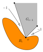
Figure 4: Illustrations for the proof of Lemma 12.

6 Concluding Remarks

We have provided an $\mathcal{O}(n^{2})$-time algorithm for testing the upward planarity of $n$-vertex directed partial $2$-trees, substantially improving on the state of the art [10]. There are several major obstacles to overcome for improving this runtime to linear; hence, it would be worth investigating whether the quadratic bound is tight. Another interesting direction for future work is to see whether our new techniques can be used to obtain quadratic algorithms for related problems, such as computing orthogonal drawings with the minimum number of bends [7, 9].

References

- [1] Bertolazzi, P., Di Battista, G., Liotta, G., Mannino, C.: Upward drawings of triconnected digraphs. Algorithmica 12(6), 476–497 (1994)
- [2] Bertolazzi, P., Di Battista, G., Mannino, C., Tamassia, R.: Optimal upward planarity testing of single-source digraphs. SIAM J. Comput. 27(1), 132–169 (1998)
- [3] Brückner, G., Himmel, M., Rutter, I.: An SPQR-tree-like embedding representation for upward planarity. In: Archambault, D., Tóth, C.D. (eds.) 27th International Symposium on Graph Drawing and Network Visualization, GD 2019. Lecture Notes in Computer Science, vol. 11904, pp. 517–531. Springer (2019)
- [4] Chan, H.Y.: A parameterized algorithm for upward planarity testing. In: Albers, S., Radzik, T. (eds.) 12th Annual European Symposium on Algorithms, ESA 2004. Lecture Notes in Computer Science, vol. 3221, pp. 157–168. Springer (2004)
- [5] Chaplick, S., Di Giacomo, E., Frati, F., Ganian, R., Raftopoulou, C.N., Simonov, K.: Parameterized algorithms for upward planarity. In: Goaoc, X., Kerber, M. (eds.) 38th International Symposium on Computational Geometry (SoCG 2022). LIPIcs, vol. 224, pp. 26:1–26:16. Schloss Dagstuhl - Leibniz-Zentrum für Informatik (2022)
- [6] Chaplick, S., Giacomo, E.D., Frati, F., Ganian, R., Raftopoulou, C.N., Simonov, K.: Testing upward planarity of partial -trees. CoRR abs/xxxx.xxxxx (2022), https://doi.org/xxxx.xxxxx
- [7] Di Battista, G., Liotta, G., Vargiu, F.: Spirality and optimal orthogonal drawings. SIAM J. Comput. 27(6), 1764–1811 (1998)
- [8] Di Battista, G., Tamassia, R.: On-line planarity testing. SIAM J. Comput. 25(5), 956–997 (1996)
- [9] Di Giacomo, E., Liotta, G., Montecchiani, F.: Orthogonal planarity testing of bounded treewidth graphs. J. Comput. Syst. Sci. 125, 129–148 (2022)
- [10] Didimo, W., Giordano, F., Liotta, G.: Upward spirality and upward planarity testing. SIAM J. Discret. Math. 23(4), 1842–1899 (2009)
- [11] Didimo, W., Liotta, G., Ortali, G., Patrignani, M.: Optimal orthogonal drawings of planar 3-graphs in linear time. In: Chawla, S. (ed.) SODA ’20. pp. 806–825. SIAM (2020)
- [12] Frati, F.: Planar rectilinear drawings of outerplanar graphs in linear time. Comput. Geom. 103, 101854 (2022)
- [13] Garg, A., Tamassia, R.: On the computational complexity of upward and rectilinear planarity testing. SIAM J. Comput. 31(2), 601–625 (2001)
- [14] Gutwenger, C., Mutzel, P.: A linear time implementation of SPQR-trees. In: Marks, J. (ed.) 8th International Symposium on Graph Drawing, GD ’00. Lecture Notes in Computer Science, vol. 1984, pp. 77–90. Springer (2000)
- [15] Healy, P., Lynch, K.: Two fixed-parameter tractable algorithms for testing upward planarity. Int. J. Found. Comput. Sci. 17(5), 1095–1114 (2006)
- [16] Hutton, M.D., Lubiw, A.: Upward planar drawing of single source acyclic digraphs. In: Aggarwal, A. (ed.) 2nd Annual ACM/SIGACT-SIAM Symposium on Discrete Algorithms, SODA 1991. pp. 203–211. ACM/SIAM (1991)
- [17] Hutton, M.D., Lubiw, A.: Upward planar drawing of single-source acyclic digraphs. SIAM J. Comput. 25(2), 291–311 (1996)
- [18] Papakostas, A.: Upward planarity testing of outerplanar dags. In: Tamassia, R., Tollis, I.G. (eds.) DIMACS International Workshop on Graph Drawing, GD ’94. Lecture Notes in Computer Science, vol. 894, pp. 298–306. Springer (1994)