Unsupervised Spike Depth Estimation via Cross-modality Cross-domain Knowledge Transfer

Abstract

Neuromorphic spike data, an upcoming modality with high temporal resolution, has shown promising potential in real-world applications due to its inherent advantage to overcome high-velocity motion blur. However, training the spike depth estimation network holds significant challenges in two aspects: sparse spatial information for dense regression tasks, and difficulties in achieving paired depth labels for temporally intensive spike streams. In this paper, we thus propose a cross-modality cross-domain (BiCross) framework to realize unsupervised spike depth estimation with the help of open-source RGB data. It first transfers cross-modality knowledge from source RGB to mediates simulated source spike data, then realizes cross-domain learning from simulated source spike to target spike data. Specifically, Coarse-to-Fine Knowledge Distillation (CFKD) is introduced to transfer cross-modality knowledge in global and pixel-level in the source domain, which complements sparse spike features by sufficient semantic knowledge of image features. We then propose Uncertainty Guided Teacher-Student (UGTS) method to realize cross-domain learning on spike target domain, ensuring domain-invariant global and pixel-level knowledge of teacher and student model through alignment and uncertainty guided depth selection measurement. To verify the effectiveness of BiCross, we conduct extensive experiments on three scenarios, including Synthetic to Real, Extreme Weather, and Scene Changing. The code and datasets will be released.

1 Introduction

The neuromorphic spike camera generates data streams with high temporal resolution in a bio-inspired way [7, 59], which has shown promising potential in real-world applications, such as autonomous driving [30, 46] and robotic manipulation [41]. Compared with RGB camera, which has severe performance degradation in the high-velocity scenario due to motion blur [21], spike camera has an inherent advantage to overcome it. Therefore, as shown in Fig. 1 (a), we attempt to realize depth estimation on spike data, which shows strengthen on dynamic objects [23].

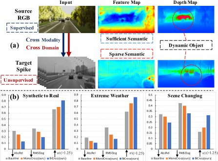
Figure 1: Part (a) demonstrates the process of BiCross and the distinct properties of RGB and spike modality. In contrast to RGB which holds sufficient semantic knowledge, spike data is not comprehensive in feature space caused by sparse spatial information. However, spike shows strength in depth estimation on dynamic objects due to its dense temporal resolution. Part (b) presents the benefits of our methods on three unsupervised transferring scenarios. Baseline is the original depth estimation method [36] without our method, MonoCross only applies cross-modality learning, BiCross learns cross-modality and cross-domain knowledge.

However, training depth estimation model on spike data with supervision is extremely unfeasible due to the intrinsic properties of spike data: (1) Dense temporal streams. Spike data is captured with high-frequency frames up to 40000 Hz, resulting in extraordinary dense temporal frames [6, 21]. Though such property can better perceive scenes of high-velocity motion blur, the annotation process becomes extremely difficult, not to mention obtaining paired depth labels for each pixel in each frame. (2) Sparse spatial information. Since spike camera adopts the firing mechanism to capture pixel-wise luminance intensity, it may sometimes miss some interactions, leading to sparse spatial information [6, 27]. It then will result in sparse semantic knowledge in feature representation, as shown in Fig. 1 (a). Meanwhile, depth prediction is a pixel-level task, the sparse spike features will lead to performance degradation when directly applying previous RGB depth estimation methods. And existing RGB-based unsupervised depth estimation methods are driven by photometric consistency [14, 29], which cannot be applied to spike streams directly.

To overcome these challenges, we propose a cross-modality cross-domain (BiCross) framework for unsupervised spike depth estimation. Since there is a huge gap between source RGB and target spike data, we simulate an intermediate source spike domain to facilitate the knowledge transferring from source RGB to target spike data. In particular, in the cross-modality phase, we propose a novel Coarse-to-Fine Knowledge Distillation (CFKD), which transfers the global and pixel-level knowledge from source RGB to simulated source spike. It complements the semantic knowledge of sparse spike data and reserves the unique strengthen of each modality, providing more available information for cross-domain transferring. During the cross-domain phase, inspired by the prevalent mean-teacher mechanism[40, 48], we introduce Uncertainty Guided Teacher-Student (UGTS) method to address the domain shift between simulated source spike and target spike in an unsupervised manner. Specifically, due to the sparse property of spike data, we adopt uncertainty measurement to screen out more reliable and task-relevant pixel-wise depth pseudo label, which are transferred from teacher to student model. Aside from the pixel-level transferred knowledge, student model further aligns global-level features of two domains, which aims to alleviate the domain shift comprehensively. Therefore, CFKD and UGTS compensate each other to realize unsupervised spike depth estimation.

We are the first to study the problem of unsupervised spike depth estimation. We conduct extensive experiments to demonstrate that our method achieves competitive performance on the new task. We design three BiCross scenarios, which are Synthetic to Real (Virtual Kitti RGB [10] to Kitti spike), Extreme Weather (normal RGB to foggy and rainy [49] spike), and Scene Changing (KITTI [13] RGB to Driving Stereo [49] spike) scenario respectively. Taking Synthetic to Real scenario as an example, as shown in Fig. 1 (b), CFKD (MonoCross) improves the semantic representation and generalization ability of spike student model and reduces AbsRel from 0.303 to 0.243. Adding UGTS further reduces AbsRel to 0.129 without any supervision.

The main contributions are summarized as follows:

1) We propose a novel cross-modality cross-domain (BiCross) framework for unsupervised spike depth estimation. We make the first attempt to exploit the open-source RGB datasets to help unsupervised spike task.

2) We introduce a Coarse-to-Fine Knowledge Distillation (CFKD) to compensate sparse spatial spike data by transferring knowledge of RGB images in global and pixel-level during cross-modality learning.

3) We introduce the Uncertainty Guided Teacher-Student (UGTS) method to generate reliable and domain-invariant depth pseudo label for student model in cross-domain phase, which addresses domain shift between two domains.

4) We conduct extensive experiment on three challenging BiCross scenarios, demonstrating the advantages and effectiveness of our method, including Synthetic to Real, Extreme Weather, and Scene Changing.

2 Related work

Monocular depth estimation Depth estimation is an important task of machine scene understanding. Deep learning has become a prevailing solution to supervised depth estimation for both outdoor [8, 13, 49] and indoor [31, 37] scenes. These methods usually consist of a general encoder to extract global context information, and a decoder to recover depth information [47, 34, 26, 35, 9]. However, the supervised methods need a mass of annotation in pixel level thus limiting their scalability and practicability. As for spike stream, it is nearly impossible to train the neural models in a supervised manner since spike stream is too temporally intensive to obtain paired depth labels. Unsupervised depth estimation methods do not require ground-truth depth to train the neural models [12, 58, 14, 15, 33, 1]. Existing unsupervised RGB depth estimation methods are driven by photometric consistency, which will cause severe performance degradation when directly applied to spike streams.

Adaptive depth estimation Existing cross-modality depth estimation methods usually take advantage of data consistency from different modalities [32, 42]. [43] proposes to use aligned DVS event data and APS images to perform cross-modality knowledge distillation for depth estimation with unaligned event data. Cross-domain depth estimation usually aligns the source and target domains from input level or feature level [25, 55, 54]. For instance, [54] developed a geometry-aware symmetric adaptation framework to jointly optimize the translation and the depth estimation network. Nevertheless, there has been no existing work jointly perform cross-modality and cross-domain depth estimation. Due to the huge gap between source RGB and target spike data, we introduce a cross-modality cross-domain (BiCross) framework to leverage the advantages from both modalities and the annotation from RGB data.

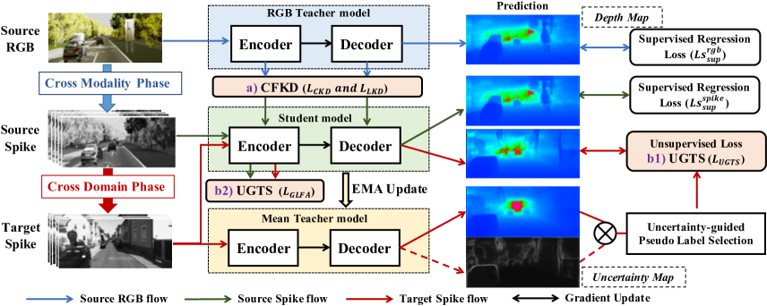
Figure 2: The framework of BiCross, which is composed of cross-modality and cross-domain phases. The first two rows demonstrate cross modality learning, we propose a noval CFKD (part a) to transfer global and pixel-level knowledge from RGB teacher model to spike student model under source domain. The last two rows introduce UGTS (part b1, b2) to transfer domain-invariant pixel-level pseudo labels from teacher to student model and jointly ease the global-level domain shift in student model. The uncertainty guided approach is conducted at the model output layer, following the two phases. CFKD and UGTS compensate each other to realize unsupervised spike depth estimation.

Spike camera and its application Spike camera is a kind of bio-inspired sensor [6] with high temporal resolution. Based on obtained spike frames from spike camera, existing works concentrate on spike-to-image reconstruction [60, 51, 56, 62, 50, 52, 61], which takes advantage of high temporal resolution of spike streams and generates high SNR as well as high frequency reconstructed images. Meanwhile, [22] proposes SCFlow to predict high-speed optical flow from spike streams. [27] proposes a retinomorphic object detection method to fuse the DVS modality and spike modality via a dynamic interaction mechanism. Compared with DVS [3, 28], spike camera adopts the firing operation to capture the pixel-wise luminance intensity instead of pixel-wise luminance change. Therefore, although both cameras are capable of reserving high temporal resolution, spike camera has more advantages for high-speed depth estimation in regions with weak and boundary textures [21]. In this paper, we make the first attempt to explore the unsupervised depth estimation for spike data and leverage the individual property of RGB and spike modalities. During inference, we only predict depth from target spike data.

3 Method

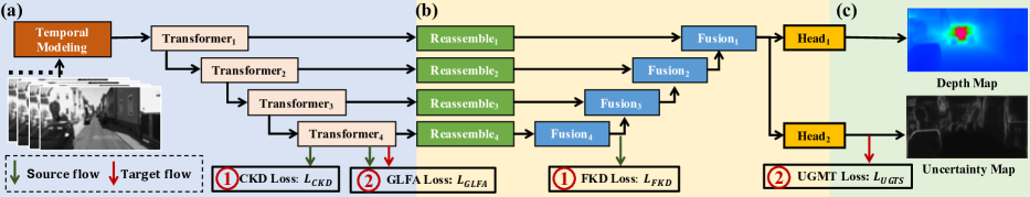
Figure 3: The detailed structure of the spike depth estimation network. The temporal spike data is sent into spike transformer encoder as shown in part (a). Part (b) and (c) represent the decoder and prediction heads of network respectively. Red circle.1 represents the objectives of cross-modality learning, including coarse (CKD) and fine-level (FKD) knowledge distillation. Red circle.2 demonstrates the objectives of cross-modality learning, which contains pseudo label transferring and global-level alignment.

We introduce the properties of neuromorphic spike data and network in Sec. 3.1. We then explain each component of BiCross framework, along with the details of two branches CFKD and UGTS in Sec. 3.2. The details of training strategy and objective functions are given in Sec. 3.3.

3.1 Neuromorphic spike data and network

3.1.1 Neuromorphic spike data

Spike camera utilizes photo receptions to capture natural lights which are converted to voltage under integration of time series $t$. Once the voltage at a certain sensing unit reaches a threshold $\Theta$, a one-bit spike is fired and the voltage is reset to zero at the same time [51].

$$\scriptstyle S(i,j,t)=\left\{\begin{array}[]{l}1,\quad\int_{{t_{0}}_{i,j}^{pre}}^{t}I(i,j)\,dt\geq\Theta\\ 0,\quad\int_{{t_{0}}_{i,j}^{pre}}^{t}I(i,j)\,dt<\Theta\end{array}\right.$$ (1)

The above formula reveals the basic working pipeline of the spike camera, where $I(i,j)$ represents the luminance of pixel $(i,j)$, and ${t_{0}}^{pre}_{i,j}$ represents the time that fires the last spike at pixel$(i,j)$. The spike fires when the accumulation of luminance reaches the threshold, capturing high frequency frames up to 40000 Hz [60, 53]. Following previous works [21, 62], we simulate and synthesize the spike frames from open source datasets under the work flow of spike camera. Then, we split the spike sequence into streams $I^{spike}=H\times W\times T$, $H$ and $W$ represent the height and width of spike frames, under the temporal resolution $T$.

3.1.2 Neuromorphic spike network

In this paper, both RGB and spike modality embed features with the help of DPT [36], where the input data are spike $I^{spike}\in\mathbb{R}^{1280\times H\times W}$ and RGB $I^{rgb}\in\mathbb{R}^{3\times H\times W}$. As shown in Fig. 3 (a), the network encoder is divided into two blocks, the first one is a temporal modeling module (SENet [20] and Resblocks [19]) to adaptively aggregate the dense temporal information of special spike data, which is utilized to reduce computational cost when the spike temporal resolution is too high (e.g., 40000 Hz). The second one is ViT-Hybrid, which uses a ResNet-50 [19] to encode the image and spike embedding followed by 12 transformer layers. In Fig. 3 (b), the decoder consists of the reassemble operation, along with the fusion module. Fig. 3 (c) contains two prediction heads, where $Head_{1}$ predicts depth and $Head_{2}$ estimates uncertainty map.

3.2 BiCross overall framework

Due to the difficulties in achieving paired spike depth data and the sparse spatial property of spike streams, we study the unsupervised spike depth estimation task by introducing open-source RGB data. As shown in Fig. 2, the overall framework contains cross-modality and cross-domain phases. We will discuss the motivation of each component and their interactions in the following.

Cross-modality learning The goal is to leverage sufficient semantic knowledge in RGB modality and compensate for the sparse spatial information in spike modality. As shown in the upper part of Fig. 2, we adopt a Coarse-to-Fine Knowledge Distillation (CFKD) to transfer the global-level representation and pixel-level task-relevant features from source RGB to mediate source spike. It reserves the unique strength of both modalities and provides more available spatial information for cross-domain transferring.

Cross-domain learning After obtaining relative comprehensive source spike representation, we introduce Uncertainty Guided Teacher-Student (UGTS) method to further transfer the knowledge from source spike to target spike and realize unsupervised spike depth estimation. As shown in the bottom part of Fig. 2, in order to alleviate domain shift between two domains, teacher model utilizes uncertainty measurement to screen out reliable depth prediction, only reserving task relevant pixel-level prediction which is transferred to student model. Student model is then trained with these domain-invariant pseudo label and thus addresses the latent domain shift. Meanwhile, the student model aligns source and target domain in global-level to jointly ease domain-specific representation.

3.2.1 Coarse-to-Fine Knowledge Distillation

We introduce the Coarse-to-Fine Knowledge Distillation (CFKD) to transfer the knowledge from RGB model $\mathcal{T}_{RGB}$ to spike model $\mathcal{S}_{src}$, which aims to align global-level representation and pixel-level task-relevant features in the phase of cross-modality. In Coarse Distillation part, we model image-spike relationships under multiple instance learning (MIL) paradigm [18], aligning encoder representation of both modalities in source domain. In our setting, positive samples are predicted from corresponding image-spike pair, while negative samples are predicted from the opposite pairs. We first aggregate the high-level feature $\mathcal{F}_{h}\in\mathbb{R}^{768\times 12\times 12}$ to obtain global level vector $\mathcal{F}_{g}\in\mathbb{R}^{256\times 1}$. We then calculate the similarity $S(\mathcal{F}_{g}^{I},\mathcal{F}_{g}^{S})\in\mathbb{R}^{1\times 1}$ between global level vector of both modalities. Practically, we calculate the similarity score of each possible image-spike pair in a batch of size b and adopt MIL to distance the similarity of corresponding and irrelevant image-spike pairs in Eq. 2.

$$\small\mathcal{L}_{CKD}(\mathcal{F}_{g_{i}}^{I},\mathcal{F}_{g_{j}}^{S})=\mathcal{E}_{\mathcal{F}_{g_{j}}^{S}\in\mathcal{S}_{B}}[b_{i,j}*log(h(\mathcal{F}_{g_{i}}^{I},\mathcal{F}_{g_{j}}^{S}))]\\$$ (2)

, where $\mathcal{S}_{B}=\{{F}_{g_{1}}^{S},..{F}_{g_{b}}^{S}\}$, $b_{i,j}=1$, if i=j, otherwise, $b_{i,j}=0$, $\tau$ is the temperature scale factor (0.5), $h$ can be formulated as Eq. 3:

$$\scriptstyle h(\mathcal{F}_{g_{i}}^{I},\mathcal{F}_{g_{j}}^{S})=\frac{exp(S(\mathcal{F}_{g_{i}}^{I},\mathcal{F}_{g_{j}}^{S})/\tau)}{exp(S(\mathcal{F}_{g_{i}}^{I},\mathcal{F}_{g_{j}}^{S})/\tau)+\sum_{\mathcal{F}_{g_{j^{\prime}}}^{S}\in\{\mathcal{S}_{B}-\mathcal{F}_{g_{j}}^{S}\}}exp(S(\mathcal{F}_{g_{i}}^{I},\mathcal{F}_{g_{j^{\prime}}}^{S})/\tau)}$$ (3)

In addition, since depth estimation problem is a collection of pixel-level regression, we thus adopt Fine Distillation to align pixel-level task-relevant features of both modalities. As shown in Fig. 3, we distill features from RGB to spike at the decoder of the network. We decrease the dispersion between every pixel in the corresponding image-spike feature pair and further transfer the abundant semantic information from RGB to spike. The loss function is given as follows:

$$\scriptstyle\mathcal{L}_{FKD}=\frac{1}{W_{l}^{\prime}\times H_{l}^{\prime}}\sum_{i\in\mathcal{P}_{l}}||d_{l,i}^{\mathcal{T}}-d_{l,i}^{\mathcal{S}}||^{2}$$ (4)

where $d_{l,i}^{\mathcal{T}}$ and $d_{l,i}^{\mathcal{S}}$ stand for the $i^{th}$ pixel value from teacher RGB model $\mathcal{T}_{RGB}$ and student spike model $\mathcal{S}_{src}$ at $l^{th}$ features, $W_{l}^{{}^{\prime}}$ and $H_{l}^{{}^{\prime}}$ stand for width and height of the distillation features at $l^{th}$ features, $\mathcal{P}_{l}=\{1,2,..,W_{l}^{\prime}\times H_{l}^{\prime}\}$. We thus shorten the features distance between model $\mathcal{T}_{RGB}$ and $\mathcal{S}_{src}$ with MSE loss. With the help of CFKD, we can leverage sufficient RGB depth labels and comprehensive spatial information from RGB modality.

3.2.2 Uncertainty Guided Teacher-Student

In the phase of cross-domain, after receiving the complemented information from RGB modality, we further deal with the domain gap between simulated source spike and target spike data. We propose Uncertainty Guided Teacher-Student (UGTS) to address domain shift in pixel and global-level. It consists of uncertainty guided teacher model $\mathcal{T}_{mean}$ with task-relevant depth selection and global-level aligned student model $\mathcal{S}_{tgt}$, which are of the same architecture.

Uncertainty guided teacher model. Due to the special property of spike data, traditional strong augmentation on student model (e.g., color conversion) will damage spike information. Therefore, we adopt a warm-up mechanism on teacher model to distance the initial weight of two models by applying a few iteration gradient updates, assisting teacher model to guide student model training. Meanwhile, the Target Student model $\mathcal{S}_{tgt}$ is updated with back-propagation, and the Mean Teacher model $\mathcal{T}_{mean}$ is updated by student’s weights with EMA. The weights of $\mathcal{T}_{mean}$ at time step $t$ is the EMA of successive $\mathcal{S}_{tgt}$,

$$\scriptstyle\mathcal{T}_{mean}^{t}=\alpha\mathcal{T}_{mean}^{t-1}+(1-\alpha)\mathcal{S}_{tgt}^{t}$$ (5)

,where $\alpha$ is a smoothing coefficient.

Then we can use the temporally ensembled teacher model to guide the student model’s training in the target domain via pseudo labels. Since the domain shift still exists in target pseudo labels, we introduce uncertainty guidance method to eliminate unreliable and more domain-specific depth pseudo labels. In contrast to uncertainty guidance, a more simple selection mechanism, which selects based on confidence score, moves decision boundaries to low-density regions in sampling-based approaches. However, it may lead to inaccuracy due to the poor calibration of neural networks and the domain gap issue will result in more severe miscalibration [16]. And different from the classification task, depth estimation is not capable to retrieve confidence score of output pseudo labels. To this end, we add an extra prediction head to estimate the uncertainty of depth estimation. We also generate soft-label for error uncertainty according to Eq. 6:

$$\scriptstyle\mathcal{E}_{soft}=\frac{|D_{pred}-D_{gt}|}{D_{gt}}$$ (6)

, where $D_{pred}$ is the output of depth prediction head and $D_{gt}$ is the depth ground-truth (in cross-modality phase) or pseudo label (in cross-domain phase) . The uncertainty estimate is penalized by Smooth L1 loss ($\mathcal{L}_{unc}$) during the two phases. With estimated uncertainty, an uncertainty-guided pseudo label valid mask $F_{mask}$ can be defined as:

$$\scriptstyle F_{mask}=\left\{\begin{array}[]{l}1,\quad\mathcal{E}_{soft}^{i}\leq\mathcal{E}_{thresh}\\ 0,\quad\mathcal{E}_{soft}^{i}>\mathcal{E}_{thresh}\end{array}\right.$$ (7)

where $\mathcal{E}_{soft}^{i}$ is the uncertainty value of the $i^{th}$ pixel and $\mathcal{E}_{thresh}$ is the variance of the uncertainty values. We adopt $\mathcal{E}_{thresh}$ to ensure the selected pseudo depth are adaptive and reliable based on the different domain shift degree of input.

Global-level aligned student model. In order to further alleviate the domain shift, aside from the pixel-level transferred pseudo label from teacher model, we introduce the Global-Level Feature Alignment (GLFA) to align features between two domains in student model. As shown in Fig. 3 (a), the GLFA is performed on the encoder outputs of the student model. Inspired by the global memory [17, 5] and the sparse attention mechanism [57, 2] in ViT encoder, we first attempt to utilize global information in spike unsupervised domain adaptation task. Particularly, We extract class token as global vectors $\mathcal{F}_{src},\mathcal{F}_{tgt}\in\mathbb{R}^{768\times 1}$ in two domains. The two global vectors are further classified by two individual domain discriminators. And we utilize the domain adversarial training method [11] to insert gradient reversal layers and reverse back-propagated gradients for domain discriminators to optimize the model in extracting global-level domain-invariant features.

3.3 Loss functions

Cross-modality loss In cross-modality learning, we update $\mathcal{T}_{RGB}$ and $\mathcal{S}_{src}$ via four losses, including RGB supervised depth estimation loss $\mathcal{L}s_{sup}^{rgb}$, source spike supervised depth estimation loss $\mathcal{L}s_{sup}^{spike}$, uncertainty estimate loss $\mathcal{L}_{unc}$, and CFKD losses ($\mathcal{L}_{CKD}$ and $\mathcal{L}_{FKD}$). Specifically, both depth estimation losses adopt Sig loss [8]. The depth estimation loss $\mathcal{L}s$ is shown as below:

$$\scriptstyle\mathcal{L}_{s}(D_{pred},D_{gt})=\frac{1}{W\times H}\sum_{i\in\mathcal{P}}L_{i}^{2}-\frac{\lambda}{(W\times H)^{2}}(\sum_{i\in\mathcal{P}}L_{i})^{2}$$ (8)

, where $L_{i}=logD_{pred}^{i}-logD_{gt}^{i}$, W and H stand for width and height of the prediction, $\mathcal{P}=\{1,2,..,W\times H\}$. The cross-modality training loss $\mathcal{L}_{Mod}$ is shown in Eq. 9.

$$\scriptstyle\mathcal{L}_{Mod}=\mathcal{L}s_{sup}^{rgb}+\mathcal{L}s_{sup}^{spike}+\mathcal{L}_{unc}+0.1*(\mathcal{L}_{CKD}+\mathcal{L}_{FKD})$$ (9)

Cross-domain loss In the cross-domain learning, we update $\mathcal{S}_{tgt}$ with loss $\mathcal{L}_{UGTS}$ under the supervision of generated pseudo labels, as shown in Eq. 10. $D_{soft}$ is the uncertainty guided pseudo label for target spike data, which is selected from depth prediction by uncertainty map $F_{mask}$

$$\scriptstyle\mathcal{L}_{UGTS}(D_{pred},D_{soft})=\frac{1}{W\times H}\sum_{i=1}^{P}smoothL1(D_{pred},D_{soft})$$ (10)

The global-level alignment loss of student model shown in Eq. 11, where ${F}_{src}$ and ${F}_{tgt}$ is the source and target spike input and $D$ denotes the domain discriminator.

$$\scriptstyle\mathcal{L}_{GLFA}({F}_{src},{F}_{tgt})=\log{D}({F}_{src})+\log(1-{D}({F}_{tgt}))$$ (11)

Therefore, the integrated cross-domain loss $\mathcal{L}_{Dom}$ is shown in Eq. 12.

$$\scriptstyle\mathcal{L}_{Dom}=\mathcal{L}_{UGTS}+0.1*\mathcal{L}_{GLFA}$$ (12)

During evaluation stage, we only use target spike data as input, and infer on trained target spike model $\mathcal{S}_{tgt}$.

Table 1: Results of different methods evaluated on Synthetic to Real scenario, from Virtual Kitti RGB to Kitti spike.

Method	Train on	Pretrain	Abs Rel ↓	Sq Rel ↓	RMSE ↓	$\delta>{1.25}$ ↑	$\delta>{1.25}^{2}$ ↑	$\delta>{1.25}^{3}$ ↑
AdaDepth[25]	VKITTI-RGB	ImageNet	0.303	2.675	9.210	0.506	0.764	0.881
T2Net[55]	VKITTI-RGB	ImageNet	0.252	2.038	5.951	0.689	0.867	0.954
SFA[44]	VKITTI-RGB	ImageNet	0.298	2.586	8.996	0.541	0.767	0.888
$Pre_{src}$	VKITTI-spike	ImageNet	0.303	3.446	7.091	0.663	0.823	0.917
MonoCross	VKITTI-spike	VKITTI-RGB	0.243	2.145	5.977	0.702	0.853	0.949
BiCross	VKITTI-spike	MonoCross	0.129	0.763	4.975	0.810	0.952	0.986
Supervised	KITTI-spike	ImageNet	0.120	0.565	3.527	0.857	0.971	0.993

4 Experiments

We conduct extensive experiments to demonstrate the effectiveness of the BiCross framework. In Sec 4.1, the details of the setup of BiCross scenarios and implementation details are given. In Sec 4.2, we evaluate the performance of our method in the three challenging BiCross scenarios, including Synthetic to Real, Extreme Weather, and Scene Changing. Comprehensive ablation studies are conducted in Sec 4.3, which investigate the impact of each component. Finally, we provide qualitative analysis to present the effectiveness of BiCross framework in Sec 4.4.

4.1 Experimental setup

Data and label acquisition In our work, we generate spike dataset using RGB frames of four open access outdoor datasets, including Kitti[13], Driving Stereo[49], Driving Stereo Weather[49], and Virtual Kitti [10]. Followed by previous work[21, 62], we use a novel video frame insertion method [39] and spike stream simulator to get spike data with 1280Hz, which reaches the real spike camera workflow. Besides, we also adopt a real spike data (Respike) as target, realizing BiCross from source NYU [38] RGB to target Respike spike data [45]. The dataset details are given in appendix, and all datasets will be released for research.

BiCross scenarios In order to promote the development of neuromorphic spike camera and evaluate the effectiveness of our method, we introduce three challenge BiCross scenarios, which are Synthetic to Real, Extreme Weather and Scene Changing. For Synthetic to Real, we set RGB Virtual Kitti as source data and realize the unsupervised depth estimation on target Kitti spike data. Virtual data considerably minimize the manual cost of data collection and annotating. For Extreme Weather, the RGB Driving Stereo in normal weather is considered as source data, foggy and rainy spike Driving Stereo is considered as target data. Variations in weather conditions are common, yet challenging, and unsupervised depth estimation must be reliable under all conditions. For Scene Changing, we design Kitti RGB as source data and transfer the knowledge to target spike Driving Stereo. Scene layouts are not static and frequently change in real-world applications, especially in autonomous driving. Due to the limitation of space, we demonstrate the Respike experiments in appendix.

Implementation details BiCross framework is built based on DPT [36]. We set ImageNet [4] pre-trained ViT-Hybrid as transformer encoder in all experiments, whereas the decoder and prediction head are initialized randomly. The structures of depth and uncertainty estimation head as same, which contain 3 convolutional layers. We set a learning rate of $1e-5$ for the backbone and $1e-4$ for the decoder. We adopt Adam optimizer [24] $(\beta_{1},\beta_{2})=(0.9,0.999)$ during cross-modality and cross-domain training for 30 and 10 epochs respectively. The batch size is set to 8 for all BiCross scenarios. For the input data, we first resize the longer side to 384 pixels and random crop a patch with 384 $\times$ 384. We only use random horizontal flip for RGB and spike data augmentation. The evaluation metrics are following previous depth estimation works [9, 36]. All experiments are conducted on NVIDIA Tesla V100 GPUs.

Table 2: Results of different methods evaluated on Extreme Weather scenario, from Driving stereo cloudy RGB to foggy and rainy spike.

			Foggy-spike			Rainy-spike
Method	Train on	Pretrain	Abs Rel ↓	RMSE ↓	$\delta>{1.25}$ ↑	Abs Rel ↓	RMSE ↓	$\delta>{1.25}$ ↑
AdaDepth[25]	Cloudy-RGB	ImageNet	0.377	20.017	0.354	0.399	20.261	0.308
T2Net[55]	Cloudy-RGB	ImageNet	0.147	9.351	0.725	0.216	10.598	0.627
SFA[44]	Cloudy-RGB	ImageNet	0.351	19.115	0.402	0.361	20.087	0.410
$Pre_{src}$	Cloudy-spike	ImageNet	0.194	11.284	0.633	0.226	12.759	0.595
MonoCross	Cloudy-spike	Cloudy-RGB	0.135	8.619	0.755	0.203	11.360	0.635
BiCross	Cloudy-spike	MonoCross	0.108	6.782	0.847	0.179	9.570	0.698
Supervised	Foggy/Rainy-spike	ImageNet	0.120	6.393	0.864	0.242	9.293	0.709

Table 3: Results of different methods evaluated on Scene Changing scenario, from KITTI RGB to DrivingStereo spike.

Method	Train on	Pretrain	Abs Rel ↓	$\delta>{1.25}$ ↑
$Pre_{src}$	KITTI-spike	ImageNet	0.322	0.160
MonoCross	KITTI-spike	KITTI-RGB	0.304	0.171
BiCross	KITTI-spike	MonoCross	0.255	0.303

4.2 The effectiveness

In this section, we compare our method against the baselines and supervised method on three BiCross scenarios. In details of method setting, $Pre_{src}$ is directly trained on simulated source spike data, MonoCross is a part of BiCross which only adopts cross-modality training, BiCross is the entire process of our method, and Supervised is trained on target spike dataset with depth label. In addition, we introduce the comparison with previous unsupervised methods, including AdaDepth [25], T2Net [55], and SFA [44] while altering their network to DPT. The selected methods can be applied to spike data and BiCross scenarios.

Synthetic to Real We select target spike sequences of Kitti that are different from source images sequence of Virtual Kitti. As shown in Tab. 1, our method can outperform other unsupervised transferring methods (i.e. AdaDepth, T2Net, and SFA), since AdaDepth and SFA can hardly align the features under an enormous gap, and T2Net is difficult to translate input data style from RGB to spike modality. BiCross even reduces 0.123 AbsRel and improves 12.2% $\delta>{1.25}$ compared with the previous SOTA methods. Meanwhile, MonoCross can exceed $Pre_{src}$ method in which CFKD reserves the advantages of two modalities and thus improves the performance on target spike data. BiCross beats all unsupervised methods by significant margins on all metrics, outperforming $Pre_{src}$ by 0.174 on AbsRel and more than 14.7% on $\delta>{1.25}$. BiCross effectively transfers sufficient knowledge from source RGB to target spike. It’s worth noting that BiCross also achieves competitive results compared with the supervised method.

Extreme Weather In order to verify the generalization of our method, we conduct an extra experiment under the scenario of extreme weather. We set cloudy RGB as source data, foggy and rainy spike streams as two different target data. As shown in Tab. 2, BiCross achieves higher accuracy than other previous unsupervised methods (AdaDepth, T2Net, and SFA) and $Pre_{src}$, showing consistent performance from Synthetic to Real scenario. To be mentioned, due to the small quantity of severe weather target data, BiCross can outperform the supervised method by 0.012 and 0.063 AbsRel in foggy and rainy target data respectively, showing great potential of our method. The results demonstrate that BiCross can transfer task relevant and semantic knowledge from open source data to target spike data, which also can achieve excellent performance on small target domain data. Besides, we conduct another extreme weather experiment in appendix, where the source data is altered to the intense light images.

Scene Changing BiCross still outperforms other methods with a considerable margin, as shown in Tab. 3. Particularly, BiCross decreases 0.067 AbsRel and 0.988 RMSE compared with $Pre_{src}$. The results demonstrate that our framework can improve the generalize ability of the spike depth model when encountering scene changing.

Table 4: Ablation studies on the Synthetic to Real scenario, from Virtual Kitti RGB to Kitti spike. It shows the effectiveness of CFKD (CKD, FKD) and UGTS (UGDS, GLFA). RGB means source RGB pretrain. In the first column, Modality means cross-modality learning, Domain means cross-domain learning, and Both means the entire phase of BiCross.

Phase	RGB	CKD	FKD	GLFA	UGDS	Abs Rel ↓	Sq Rel ↓	RMSE ↓	$\delta>{1.25}$ ↑	$\delta>{1.25}^{2}$ ↑	$\delta>{1.25}^{3}$ ↑
$Pre_{src}$	-	-	-	-	-	0.294	3.359	7.303	0.658	0.835	0.926
$Pre_{srcRGB}$	✓	-	-	-	-	0.275	2.353	6.142	0.671	0.846	0.947
Modality ($Ex_{1}$)	✓	✓	-	-	-	0.260	2.159	6.043	0.681	0.856	0.953
Modality ($Ex_{2}$)	✓	-	✓	-	-	0.266	2.355	6.061	0.679	0.840	0.940
Modality ($Ex_{3}$)	✓	✓	✓	-	-	0.243	2.145	5.977	0.702	0.853	0.949
Domain ($Ex_{4}$)	-	-	-	✓	-	0.237	1.671	6.114	0.688	0.866	0.947
Domain ($Ex_{5}$)	-	-	-	-	✓	0.230	1.790	5.487	0.707	0.877	0.955
Domain ($Ex_{6}$)	-	-	-	✓	✓	0.205	1.403	5.241	0.740	0.900	0.968
Both ($Ex_{7}$)	✓	✓	✓	✓	-	0.174	1.057	5.360	0.747	0.918	0.979
Both ($Ex_{8}$)	✓	✓	✓	-	MT	0.216	1.627	5.517	0.736	0.892	0.961
Both ($Ex_{9}$)	✓	✓	✓	-	✓	0.162	0.961	5.395	0.785	0.942	0.984
Both ($Ex_{10}$)	✓	✓	✓	✓	✓	0.129	0.763	4.975	0.810	0.952	0.986

4.3 Ablation study

In this subsection, we evaluate the contribution of each component in BiCross on Synthetic to Real scenario. In particular, BiCross contains CFKD in cross-modality phase and UGTS in cross-domain phase. UGTS contains an uncertainty guided depth selection (UGDS) method in teacher model and a global-level feature alignment (GLFA) method in student model. And we can divide CFKD into Coarse (CKD) and Fine Knowledge Distillation (FKD). We also carry out consistent ablation studies on Extreme Weather scenario in appendix.

Effectiveness of each component As shown in Tab. 4, the first two rows demonstrate the $Pre_{src}$ and $Pre_{srcRGB}$ with pretrain on virtual source RGB. As we can see, RGB modality can enhance the ability of spike depth estimation in target domain. In modality phase, $Ex_{1}$ and $Ex_{2}$ verify the effectiveness of CKD and FKD method respectively, $Ex_{3}$ (CFKD) outperforms $Pre_{srcRGB}$ by 0.032 AbsRel. This means the cross-modality phase can improve the generalization ability of model on target spike. And in domain phase, without pretrain on source RGB, we evaluate UGDS and GLFA on $Ex_{4}$ and $Ex_{5}$ individually, which achieve promising results on target spike. Compared with $Pre_{src}$, $Ex_{6}$ decreases the AbsRel from 0.294 to 0.205, demonstrating the methods can further address the domain shift. From $Ex_{7}$ to $Ex_{10}$, based on CFKD, we progressively add UGDS and GLFA methods in BiCross training. Obviously, $Ex_{7}$ and $Ex_{9}$ achieve better performance than above all methods, and $Ex_{10}$ further improves the depth estimation accuracy, which verifies the effectiveness of BiCross.

Effectiveness of uncertainty guidance We conduct more detailed experiments on UGTS to verify the effectiveness of uncertainty guided operation. In Tab. 4, since unreliable and domain-specific pseudo labels are not eliminated, $Ex_{8}$ (only using mean-teacher mechanism) can only achieve partial improvement than $Ex_{3}$ (MonoCross). However, $Ex_{9}$ (UGTS) outperforms MonoCross and $Ex_{8}$ by 0.081 and 0.054 AbsRel respectively, which demonstrates that uncertainty guided depth selection (UGDS) can alleviate the domain shift in pixel-level.

4.4 Qualitative analysis

We show the qualitative comparison of features and outputs in Fig. 5 and Fig. 4 respectively. As shown in Fig. 5, there is an object (car) in red circle but only background in blue circle. We notice that CFKD (b) can obviously improves the semantic representation of student model, which concentrates more on the foreground object. BiCross (c) further improves the feature representation of student model, which reduces the influence of domain-specific background in blue circle. The results verify that our methods can improve domain-invariant feature representation during cross-modality and cross-domain learning. As shown in Fig. 4, our method can estimate better depth map compared with others, which demonstrates that our method can effectively transfer knowledge from source RGB to target spike data. Note that, the uncertainty map for pixel-level pseudo label selection also achieves satisfying results.

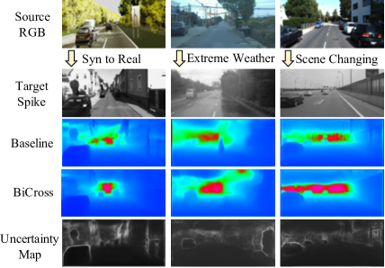
Figure 4: Quantitative results. Baseline represents the output of $Pre_{src}$. Uncertainty Map is predicted by our method in unsupervised cross-domain phase. Best viewed by zooming x4.

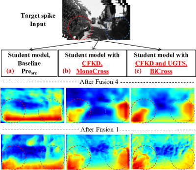
Figure 5: Quantitative features. All the methods are only trained on source domain data, and the features are extracted after Fusion 1 and 4 module during target spike domain inference. The methods are $Pre_{src}$ (a), MonoCross (b), and BiCross (c).

Table 5: The partitioning and details of Spike datasets. Count means the number of spike frames in spike datasets.

Scenario	Dataset	Training sequences	Count	Test sequences	Count
	Virtual Kitti	all training sequences	229k	all test sequences	43k
		2011_09_26_drive_0019_sync
		2011_09_26_drive_0023_sync
Syn to Real	Partial Kitti	2011_09_26_drive_0035_sync	242k	2011_09_26_drive_0039_sync	49k
		2011_09_26_drive_0046_sync
		2011_09_26_drive_0064_sync
		2011_09_30_drive_0020_sync
		80% of sunny sequences	51k
Extreme Weather	Driving Stereo Weather	80% of cloudy sequences	51k
		80% of rainy sequences	51k	20% of rainy sequence	13k
		80% of foggy sequences	51k	20% of foggy sequence	13k
	All Kitti	all training sequences	2964k	all test sequences	83k
		2018_07_31_11_07_48
		2018_07_31_11_22_31
		2018_08_17_09_45_58
Scene Changes	Partial Driving Stereo	2018_10_11_17_08_31	2968k	2018_08_01_11_13_14	196k
		2018_10_16_11_13_47
		2018_10_17_14_35_33
		2018_10_17_15_38_01
		2018_10_24_11_01_00
	NYUv2	all training sequences	102k	all test sequences	89k
Respike	Respike [45]	all indoor sequences	45k	indoor test sequences	6k

5 Conclusion and discussion of limitations

We are the first to explore the unsupervised task in spike modality, and we propose a novel BiCross framework to exploit the multi-level knowledge of open-source RGB datasets and reserve the advantages of both modalities. For the cross-modality phase, Coarse-to-Fine Knowledge Distillation transfers the global and pixel-level knowledge from source RGB to simulated source spike. For the cross-domain phase, we introduce Uncertainty Guided Teacher-Student to align the global-level features between two domains and transfer pixel-level domain-invariant pseudo labels. In order to pave the way for unsupervised spike depth estimation, we translate wildly used RGB depth datasets to spike modality and demonstrate the effectiveness and generalization ability of BiCross. For limitations, due to the teacher-student mechanism, BiCross brings more computational cost during training. However, when inference on target spike data, the parameters and forward propagate time of student model has not been increased.

6 Appendix

In the supplementary material, we first demonstrate more details of our spike datasets in Sec. 6.1, which is a series of open-source and practical spike depth estimation datasets. Secondly, in Sec. 6.2, we then provide additional and detailed cross-modality and cross-domain training strategy. In Sec. 6.3, we compare our method against the baselines and supervised method on Extreme Weather (from intense light RGB to foggy and rainy spike) and Real spike (Respike) scenarios. For Respike scenario, BiCross transfers knowledge from source NYU [38] RGB to target Respike indoor spike [45]. Then, we provide an additional ablation study on Extreme Weather scenario (from cloudy RGB to foggy spike) and further introduce more metrics to evaluate. Finally, in Sec. 6.4, we show more quality results in three challenging scenarios.

Table 6: Results of different methods evaluating on Extreme Weather scenario, from intense light RGB [49] to foggy and rainy spike.

			Foggy-spike			Rainy-spike
Method	Train on	Pretrain	Abs Rel ↓	RMSE ↓	$\delta>{1.25}$ ↑	Abs Rel ↓	RMSE ↓	$\delta>{1.25}$ ↑
AdaDepth[25]	Sunny-RGB	ImageNet	0.390	20.158	0.339	0.422	21.502	0.281
T2Net[55]	Sunny-RGB	ImageNet	0.156	9.085	0.712	0.215	11.887	0.621
SFA[44]	Sunny-RGB	ImageNet	0.368	19.541	0.375	0.397	21.143	0.326
$Pre_{src}$	Sunny-spike	ImageNet	0.218	11.697	0.562	0.255	13.475	0.541
MonoCross	Sunny-spike	Sunny-RGB	0.154	8.990	0.712	0.242	12.667	0.577
BiCross	Sunny-spike	MonoCross	0.110	7.298	0.826	0.203	9.839	0.674
Supervised	Foggy/Rainy-spike	ImageNet	0.120	6.393	0.864	0.242	9.293	0.709

Table 7: Results of our proposed methods evaluating on Respike scenario, from NYUv2 RGB to Respike indoor spike data.

Method	Train on	Pretrain	Abs Rel ↓	RMSE ↓	$\delta>{1.25}$ ↑
$Pre_{src}$	NYU-spike	ImageNet	0.372	0.536	0.450
MonoCross	NYU-spike	NYU-RGB	0.337	0.473	0.447
BiCross	NYU-spike	MonoCross	0.225	0.302	0.711

Table 8: Ablation studies on the Extreme Weather scenario, from cloudy RGB to foggy spike data. It shows the effectiveness of CFKD (CKD, FKD) and UGTS (UGDS, GLFA). RGB means source RGB pretrain. In the first column, Modality means cross-modality learning, Domain means cross-domain learning, and Both means the entire phase of BiCross.

Phase	RGB	CKD	FKD	GLFA	UGDS	Abs Rel ↓	Sq Rel ↓	RMSE ↓	$\delta>{1.25}$ ↑	$\delta>{1.25}^{2}$ ↑	$\delta>{1.25}^{3}$ ↑
$Pre_{src}$	-	-	-	-	-	0.194	2.899	11.284	0.633	0.799	0.905
$Pre_{srcRGB}$	✓	-	-	-	-	0.150	1.804	8.823	0.729	0.896	0.964
Modality ($Ex_{1}$)	✓	✓	-	-	-	0.146	1.712	8.988	0.735	0.900	0.964
Modality ($Ex_{2}$)	✓	-	✓	-	-	0.145	1.739	9.116	0.735	0.898	0.965
Modality ($Ex_{3}$)	✓	✓	✓	-	-	0.135	1.641	8.619	0.755	0.915	0.969
Domain ($Ex_{4}$)	-	-	-	✓	-	0.178	2.409	10.193	0.697	0.844	0.935
Domain ($Ex_{5}$)	-	-	-	-	✓	0.181	2.589	10.674	0.658	0.831	0.930
Domain ($Ex_{6}$)	-	-	-	✓	✓	0.172	2.114	9.299	0.735	0.876	0.949
Both ($Ex_{7}$)	✓	✓	✓	✓	-	0.129	1.533	8.276	0.775	0.924	0.972
Both ($Ex_{8}$)	✓	✓	✓	-	MT	0.131	1.586	8.207	0.766	0.921	0.976
Both ($Ex_{9}$)	✓	✓	✓	-	✓	0.127	1.427	8.012	0.794	0.932	0.978
Both ($Ex_{10}$)	✓	✓	✓	✓	✓	0.108	1.175	6.782	0.847	0.944	0.974

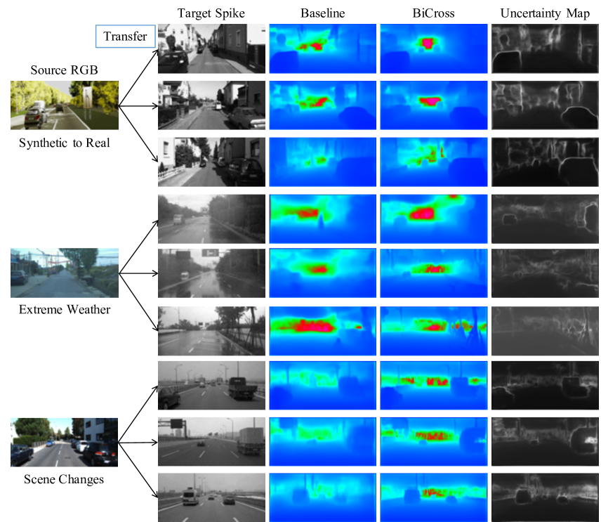
Figure 6: Qualitative results. Baseline represents the output of $Pre_{src}$. Uncertainty Map is predicted by our method in unsupervised cross-domain phase. Best viewed by zooming x4.

6.1 Additional details of spike datasets

In this paper, we generate spike datasets with RGB frames of five open access datasets, including Kitti[13], Driving Stereo[49], Driving Stereo Weather[49], Virtual Kitti [10], and NYUv2[38]. Following previous works [21, 62], we utilize the spike stream simulator to generate spike data of 1280Hz, which equals to the real spike camera workflow. As shown in Tab. 5, for these five open-source datasets, we generate spike streams of all sequences in original RGB datasets. In particular, for Synthetic to Real scenario, we transfer knowledge from Virtual Kitti source RGB to Partial Kitti target spike. We set Kitti RGB as source data and partial Driving Stereo spike as target data in Scene Changes scenario. In addition, we select 10% samples of the training dataset to constitute the validation dataset.

6.2 Additional implementation details

Our training process of BiCross can be mainly divided into 3 stages: pretraining, cross-modality training, and cross-domain training. First, in order to better adapt the model to the task of depth estimation, we load the DPT of ImageNet [4] pretrained parameters to train 30 epochs on source RGB. Then, we load the DPT parameters pretrained on source RGB into both the RGB and the spike models to conduct cross-modality training of another 10 epochs. After that, we move on to cross-domain training. Here we choose to alternate GLFA and UGDS training for 10 epochs each, 20 epochs in total. We have also tried to combine the two ways of training, but the training of GLFA led to the unstable updating of the teacher model and further led to the inaccuracy of pseudo labels, thus leading to sub-optimal performance. Finally, we directly test the student model on target spike as the result of BiCross.

6.3 Supplementary Experimental Analysis

We conduct extra experiments to demonstrate the effectiveness of the BiCross framework. The setup of BiCross scenarios and implementation details are introduced in the submission. In Sec. 6.3.1, we evaluate the performance of our proposed method in the additional two challenging BiCross scenarios, including Extreme Weather (from intense light RGB to foggy and rainy spike data) and Respike (from NYUv2 RGB to Respike indoor spike data). Additional ablation studies are conducted on Extreme weather scenario in Sec. 6.3.2, which investigate the impact of each component.

6.3.1 Additional effectiveness

In this subsection, we further conduct extensive experiments to evaluate our method on two BiCross scenarios. $Pre_{src}$ is trained on source spike with ImageNet pretrain, MonoCross is a part of our method which only adopts cross-modality training, BiCross is the entire process of our method, and Supervised is trained on target spike dataset with depth label. In addition, we keep the unsupervised training strategy of AdaDepth [25], T2Net [55], and SFA[44] while altering their depth estimation network to DPT, which are trained on source RGB.

Extreme Weather In order to verify the generalization ability of our method, we conduct experiments under the scenario of Extreme Weather. Different from Extreme Weather experiment in submission, we alter source data to the images of intense light and still utilize foggy and rainy spike streams as two different target data. As shown in Tab. 6, our method can outperform other unsupervised transferring methods (i.e. AdaDepth, T2Net, and SFA), since AdaDepth and SFA can hardly align the features under the enormous gap of cross-modality. Since spike data is a unique modality and holds dense temporal resolution, T2Net is difficult to translate input data style from RGB to spike. The results of MonoCross and BiCross evaluate the effectiveness of our cross-modality and cross-domain learning, showing the great potential of our methods. Compared with the supervised method, BiCross achieves promising results, decreasing 0.01 and 0.04 AbsRel in foggy and rainy target data respectively.

Respike We set NYUv2 [38] as source RGB and transfer the knowledge to Respike target spike data [45]. As shown in Tab. 7, BiCross beats the baseline method ($Pre_{src}$) and MonoCross by significant margins on all metrics, outperforming $Pre_{src}$ by 0.147 on AbsRel and more than 0.261% on $\delta>{1.25}$. Meanwhile, since source NYU spike is generated by our spike simulator and target spike is captured by real spike cameras, the experiment results verify that there is no different data distribution between real and simulated spike data.

6.3.2 Additional ablation study on Extreme Weather

In this subsection, we intend to evaluate the contribution of each component in BiCross on Extreme Weather scenario, which is from cloudy source RGB to foggy target spike. Same with the submission, BiCross contains CFKD in cross-modality phase, and UGMT and GLFA in cross-domain phase. We divide CFKD into Coarse (CKD) and Fine Knowledge Distillation (FKD). As shown in Tab. 8, the first two rows are $Pre_{src}$ and $Pre_{srcRGB}$ with cloudy source RGB pretrain. The results show that source RGB modality can help to improve the ability of representation and cross-domain in spike depth estimation. $Ex_{1}$ and $Ex_{2}$ demonstrate the effectiveness of CKD and FKD methods respectively in cross-modality phase, and the entire CFKD ($Ex_{3}$) can outperform $Pre_{srcRGB}$ by 0.015 AbsRel. This means cross-modality phase can improve the generalization ability of depth model on target spike. For cross-domain phase, without pretrain on source RGB, we evaluate GLFA and UGMT on $Ex_{4}$ and $Ex_{5}$ individually, improving the AbsRel to 0.178 and 0.181 on target spike. Compared with $Pre_{src}$, the entire cross-domain method ($Ex_{6}$) decreases the AbsRel from 0.194 to 0.172, verifying the methods of cross-domain phase are valid and compensatory. From $Ex_{7}$ to $Ex_{10}$, based on CFKD, we gradually add GLFA and UGMT methods in BiCross training. Same with the results in submission, $Ex_{7}$ and $Ex_{9}$ achieve better performance than all above methods, and $Ex_{10}$ further improves the depth estimation accuracy, which verifies the effectiveness of BiCross framework. However, $Ex_{8}$ (MT) can only achieve partial improvement compared with $Ex_{3}$ (MonoCross), which demonstrates the necessity of uncertainty-guided pseudo label selection.

6.4 Additional visualization and analysis

As shown in Fig. 6, we show some visualization results in three challenging BiCross scenarios, including Synthetic to Real (line 1-3), Extreme Weather (line 4-6), and Scene Changes (line 7-9). As shown in the first two columns, there is an enormous distribution gap from source RGB to target spike. Note that, BiCross can achieve better predictions than Baseline method, and improve the ability of depth estimation in the region of edge, sharp, and distance. The last column is the visualization of uncertainty map, which is predicted by BiCross framework in unsupervised cross-domain phase. Obviously, the uncertainty value of central part of an object is lower than the edge of the object, and the uncertainty value of short-distance pixels is lower than long-distance pixels.

References

- [1] Zhi Chen, Xiaoqing Ye, Wei Yang, Zhenbo Xu, Xiao Tan, Zhikang Zou, Errui Ding, Xinming Zhang, and Liusheng Huang. Revealing the reciprocal relations between self-supervised stereo and monocular depth estimation. In Proceedings of the IEEE/CVF International Conference on Computer Vision, pages 15529–15538, 2021.
- [2] Rewon Child, Scott Gray, Alec Radford, and Ilya Sutskever. Generating long sequences with sparse transformers. arXiv preprint arXiv:1904.10509, 2019.
- [3] Tobi Delbrück, Bernabe Linares-Barranco, Eugenio Culurciello, and Christoph Posch. Activity-driven, event-based vision sensors. In Proceedings of 2010 IEEE international symposium on circuits and systems, pages 2426–2429. IEEE, 2010.
- [4] Jia Deng, Wei Dong, Richard Socher, Li-Jia Li, Kai Li, and Li Fei-Fei. Imagenet: A large-scale hierarchical image database. In 2009 IEEE conference on computer vision and pattern recognition, pages 248–255. Ieee, 2009.
- [5] Jacob Devlin, Ming-Wei Chang, Kenton Lee, and Kristina Toutanova. Bert: Pre-training of deep bidirectional transformers for language understanding. arXiv preprint arXiv:1810.04805, 2018.
- [6] Siwei Dong, Tiejun Huang, and Yonghong Tian. Spike camera and its coding methods. arXiv preprint arXiv:2104.04669, 2021.
- [7] Siwei Dong, Lin Zhu, Daoyuan Xu, Yonghong Tian, and Tiejun Huang. An efficient coding method for spike camera using inter-spike intervals. arXiv preprint arXiv:1912.09669, 2019.
- [8] David Eigen, Christian Puhrsch, and Rob Fergus. Depth map prediction from a single image using a multi-scale deep network. Advances in neural information processing systems, 27, 2014.
- [9] Huan Fu, Mingming Gong, Chaohui Wang, Kayhan Batmanghelich, and Dacheng Tao. Deep ordinal regression network for monocular depth estimation. In Proceedings of the IEEE conference on computer vision and pattern recognition, pages 2002–2011, 2018.
- [10] Adrien Gaidon, Qiao Wang, Yohann Cabon, and Eleonora Vig. Virtual worlds as proxy for multi-object tracking analysis. In Proceedings of the IEEE conference on computer vision and pattern recognition, pages 4340–4349, 2016.
- [11] Yaroslav Ganin, Evgeniya Ustinova, Hana Ajakan, Pascal Germain, Hugo Larochelle, François Laviolette, Mario Marchand, and Victor Lempitsky. Domain-adversarial training of neural networks. The journal of machine learning research, 17(1):2096–2030, 2016.
- [12] Ravi Garg, Vijay Kumar Bg, Gustavo Carneiro, and Ian Reid. Unsupervised cnn for single view depth estimation: Geometry to the rescue. In European conference on computer vision, pages 740–756. Springer, 2016.
- [13] Andreas Geiger, Philip Lenz, and Raquel Urtasun. Are we ready for autonomous driving? the kitti vision benchmark suite. In 2012 IEEE conference on computer vision and pattern recognition, pages 3354–3361. IEEE, 2012.
- [14] Clément Godard, Oisin Mac Aodha, and Gabriel J Brostow. Unsupervised monocular depth estimation with left-right consistency. In Proceedings of the IEEE conference on computer vision and pattern recognition, pages 270–279, 2017.
- [15] Clément Godard, Oisin Mac Aodha, Michael Firman, and Gabriel J Brostow. Digging into self-supervised monocular depth estimation. In Proceedings of the IEEE/CVF International Conference on Computer Vision, pages 3828–3838, 2019.
- [16] Chuan Guo, Geoff Pleiss, Yu Sun, and Kilian Q Weinberger. On calibration of modern neural networks. In International conference on machine learning, pages 1321–1330. PMLR, 2017.
- [17] Qipeng Guo, Xipeng Qiu, Pengfei Liu, Yunfan Shao, Xiangyang Xue, and Zheng Zhang. Star-transformer. arXiv preprint arXiv:1902.09113, 2019.
- [18] Michael Gutmann and Aapo Hyvärinen. Noise-contrastive estimation: A new estimation principle for unnormalized statistical models. In Proceedings of the thirteenth international conference on artificial intelligence and statistics, pages 297–304. JMLR Workshop and Conference Proceedings, 2010.
- [19] Kaiming He, Xiangyu Zhang, Shaoqing Ren, and Jian Sun. Deep residual learning for image recognition. In Proceedings of the IEEE conference on computer vision and pattern recognition, pages 770–778, 2016.
- [20] Jie Hu, Li Shen, and Gang Sun. Squeeze-and-excitation networks. In Proceedings of the IEEE conference on computer vision and pattern recognition, pages 7132–7141, 2018.
- [21] Liwen Hu, Rui Zhao, Ziluo Ding, Lei Ma, Boxin Shi, Ruiqin Xiong, and Tiejun Huang. Optical flow estimation for spiking camera. arXiv preprint arXiv:2110.03916, 2021.
- [22] Liwen Hu, Rui Zhao, Ziluo Ding, Ruiqin Xiong, Lei Ma, and Tiejun Huang. Scflow: Optical flow estimation for spiking camera. arXiv preprint arXiv:2110.03916, 2021.
- [23] Zhe Hu, Li Xu, and Ming-Hsuan Yang. Joint depth estimation and camera shake removal from single blurry image. In Proceedings of the IEEE Conference on Computer Vision and Pattern Recognition, pages 2893–2900, 2014.
- [24] Diederik P Kingma and Jimmy Ba. Adam: A method for stochastic optimization. arXiv preprint arXiv:1412.6980, 2014.
- [25] Jogendra Nath Kundu, Phani Krishna Uppala, Anuj Pahuja, and R Venkatesh Babu. Adadepth: Unsupervised content congruent adaptation for depth estimation. In Proceedings of the IEEE conference on computer vision and pattern recognition, pages 2656–2665, 2018.
- [26] Jae-Han Lee and Chang-Su Kim. Monocular depth estimation using relative depth maps. In Proceedings of the IEEE/CVF Conference on Computer Vision and Pattern Recognition, pages 9729–9738, 2019.
- [27] Jianing Li, Xiao Wang, Lin Zhu, Jia Li, Tiejun Huang, and Yonghong Tian. Retinomorphic object detection in asynchronous visual streams. 2022.
- [28] Patrick Lichtsteiner, Christoph Posch, and Tobi Delbruck. A 128 x 128 120 db 15x1e-6 s latency asynchronous temporal contrast vision sensor. IEEE journal of solid-state circuits, 43(2):566–576, 2008.
- [29] Adrian Lopez-Rodriguez and Krystian Mikolajczyk. Desc: Domain adaptation for depth estimation via semantic consistency. arXiv preprint arXiv:2009.01579, 2020.
- [30] Fabian Manhardt, Wadim Kehl, and Adrien Gaidon. Roi-10d: Monocular lifting of 2d detection to 6d pose and metric shape. In Proceedings of the IEEE/CVF Conference on Computer Vision and Pattern Recognition, pages 2069–2078, 2019.
- [31] Pushmeet Kohli Nathan Silberman, Derek Hoiem and Rob Fergus. Indoor segmentation and support inference from rgbd images. In ECCV, 2012.
- [32] Yongri Piao, Xinxin Ji, Miao Zhang, and Yukun Zhang. Learning multi-modal information for robust light field depth estimation. arXiv preprint arXiv:2104.05971, 2021.
- [33] Andrea Pilzer, Stephane Lathuiliere, Nicu Sebe, and Elisa Ricci. Refine and distill: Exploiting cycle-inconsistency and knowledge distillation for unsupervised monocular depth estimation. In Proceedings of the IEEE/CVF Conference on Computer Vision and Pattern Recognition, pages 9768–9777, 2019.
- [34] Michael Ramamonjisoa, Yuming Du, and Vincent Lepetit. Predicting sharp and accurate occlusion boundaries in monocular depth estimation using displacement fields. In Proceedings of the IEEE/CVF Conference on Computer Vision and Pattern Recognition (CVPR), June 2020.
- [35] Michael Ramamonjisoa and Vincent Lepetit. Sharpnet: Fast and accurate recovery of occluding contours in monocular depth estimation. In Proceedings of the IEEE/CVF International Conference on Computer Vision (ICCV) Workshops, Oct 2019.
- [36] René Ranftl, Alexey Bochkovskiy, and Vladlen Koltun. Vision transformers for dense prediction. In Proceedings of the IEEE/CVF International Conference on Computer Vision, pages 12179–12188, 2021.
- [37] Daniel Scharstein, Heiko Hirschmüller, York Kitajima, Greg Krathwohl, Nera Nešić, Xi Wang, and Porter Westling. High-resolution stereo datasets with subpixel-accurate ground truth. In German conference on pattern recognition, pages 31–42. Springer, 2014.
- [38] Nathan Silberman, Derek Hoiem, Pushmeet Kohli, and Rob Fergus. Indoor segmentation and support inference from rgbd images. In European conference on computer vision, pages 746–760. Springer, 2012.
- [39] Hyeonjun Sim, Jihyong Oh, and Munchurl Kim. Xvfi: Extreme video frame interpolation. In Proceedings of the IEEE/CVF International Conference on Computer Vision, pages 14489–14498, 2021.
- [40] Kihyuk Sohn, Zizhao Zhang, Chun-Liang Li, Han Zhang, Chen-Yu Lee, and Tomas Pfister. A simple semi-supervised learning framework for object detection. arXiv preprint arXiv:2005.04757, 2020.
- [41] Jonathan Tremblay, Thang To, Balakumar Sundaralingam, Yu Xiang, Dieter Fox, and Stan Birchfield. Deep object pose estimation for semantic robotic grasping of household objects. arXiv preprint arXiv:1809.10790, 2018.
- [42] Yannick Verdié, Jifei Song, Barnabé Mas, Benjamin Busam, Aleš Leonardis, and Steven McDonagh. Cromo: Cross-modal learning for monocular depth estimation. arXiv preprint arXiv:2203.12485, 2022.
- [43] Lin Wang, Yujeong Chae, Sung-Hoon Yoon, Tae-Kyun Kim, and Kuk-Jin Yoon. Evdistill: Asynchronous events to end-task learning via bidirectional reconstruction-guided cross-modal knowledge distillation. In Proceedings of the IEEE/CVF Conference on Computer Vision and Pattern Recognition, pages 608–619, 2021.
- [44] Wen Wang, Yang Cao, Jing Zhang, Fengxiang He, Zheng-Jun Zha, Yonggang Wen, and Dacheng Tao. Exploring sequence feature alignment for domain adaptive detection transformers. In Proceedings of the 29th ACM International Conference on Multimedia, pages 1730–1738, 2021.
- [45] Yixuan Wang, Jianing Li, Linlin Zhu, Xijie Xiang, Tiejun Huang, and Yonghong Tian. Learning stereo depth estimation with bio-inspired spike cameras. In 2022 IEEE International Conference on Multimedia and Expo (ICME). IEEE, 2022.
- [46] Di Wu, Zhaoyong Zhuang, Canqun Xiang, Wenbin Zou, and Xia Li. 6d-vnet: End-to-end 6-dof vehicle pose estimation from monocular rgb images. In Proceedings of the IEEE/CVF Conference on Computer Vision and Pattern Recognition Workshops, pages 0–0, 2019.
- [47] Dan Xu, Wei Wang, Hao Tang, Hong Liu, Nicu Sebe, and Elisa Ricci. Structured attention guided convolutional neural fields for monocular depth estimation. In Proceedings of the IEEE Conference on Computer Vision and Pattern Recognition (CVPR), June 2018.
- [48] Mengde Xu, Zheng Zhang, Han Hu, Jianfeng Wang, Lijuan Wang, Fangyun Wei, Xiang Bai, and Zicheng Liu. End-to-end semi-supervised object detection with soft teacher. In Proceedings of the IEEE/CVF International Conference on Computer Vision, pages 3060–3069, 2021.
- [49] Guorun Yang, Xiao Song, Chaoqin Huang, Zhidong Deng, Jianping Shi, and Bolei Zhou. Drivingstereo: A large-scale dataset for stereo matching in autonomous driving scenarios. In Proceedings of the IEEE/CVF Conference on Computer Vision and Pattern Recognition, pages 899–908, 2019.
- [50] Jing Zhao, Jiyu Xie, Ruiqin Xiong, Jian Zhang, Zhaofei Yu, and Tiejun Huang. Super resolve dynamic scene from continuous spike streams. In Proceedings of the IEEE/CVF International Conference on Computer Vision, pages 2533–2542, 2021.
- [51] Jing Zhao, Ruiqin Xiong, and Tiejun Huang. High-speed motion scene reconstruction for spike camera via motion aligned filtering. In 2020 IEEE International Symposium on Circuits and Systems (ISCAS), pages 1–5, 2020.
- [52] Jing Zhao, Ruiqin Xiong, Hangfan Liu, Jian Zhang, and Tiejun Huang. Spk2imgnet: Learning to reconstruct dynamic scene from continuous spike stream. In Proceedings of the IEEE/CVF Conference on Computer Vision and Pattern Recognition, pages 11996–12005, 2021.
- [53] Jing Zhao, Ruiqin Xiong, Hangfan Liu, Jian Zhang, and Tiejun Huang. Spk2imgnet: Learning to reconstruct dynamic scene from continuous spike stream. In Proceedings of the IEEE/CVF Conference on Computer Vision and Pattern Recognition (CVPR), pages 11996–12005, June 2021.
- [54] Shanshan Zhao, Huan Fu, Mingming Gong, and Dacheng Tao. Geometry-aware symmetric domain adaptation for monocular depth estimation. In Proceedings of the IEEE/CVF Conference on Computer Vision and Pattern Recognition, pages 9788–9798, 2019.
- [55] Chuanxia Zheng, Tat-Jen Cham, and Jianfei Cai. T2net: Synthetic-to-realistic translation for solving single-image depth estimation tasks. In Proceedings of the European conference on computer vision (ECCV), pages 767–783, 2018.
- [56] Yajing Zheng, Lingxiao Zheng, Zhaofei Yu, Boxin Shi, Yonghong Tian, and Tiejun Huang. High-speed image reconstruction through short-term plasticity for spiking cameras. In Proceedings of the IEEE/CVF Conference on Computer Vision and Pattern Recognition, pages 6358–6367, 2021.
- [57] Haoyi Zhou, Shanghang Zhang, Jieqi Peng, Shuai Zhang, Jianxin Li, Hui Xiong, and Wancai Zhang. Informer: Beyond efficient transformer for long sequence time-series forecasting. In Proceedings of the AAAI Conference on Artificial Intelligence, volume 35, pages 11106–11115, 2021.
- [58] Tinghui Zhou, Matthew Brown, Noah Snavely, and David G Lowe. Unsupervised learning of depth and ego-motion from video. In Proceedings of the IEEE conference on computer vision and pattern recognition, pages 1851–1858, 2017.
- [59] Lin Zhu, Siwei Dong, Tiejun Huang, and Yonghong Tian. A retina-inspired sampling method for visual texture reconstruction. In 2019 IEEE International Conference on Multimedia and Expo (ICME), pages 1432–1437. IEEE, 2019.
- [60] Lin Zhu, Siwei Dong, Jianing Li, Tiejun Huang, and Yonghong Tian. Retina-like visual image reconstruction via spiking neural model. In Proceedings of the IEEE/CVF Conference on Computer Vision and Pattern Recognition, pages 1438–1446, 2020.
- [61] Lin Zhu, Siwei Dong, Jianing Li, Tiejun Huang, and Yonghong Tian. Ultra-high temporal resolution visual reconstruction from a fovea-like spike camera via spiking neuron model. IEEE Transactions on Pattern Analysis and Machine Intelligence, 2022.
- [62] Lin Zhu, Jianing Li, Xiao Wang, Tiejun Huang, and Yonghong Tian. Neuspike-net: High speed video reconstruction via bio-inspired neuromorphic cameras. In Proceedings of the IEEE/CVF International Conference on Computer Vision, pages 2400–2409, 2021.