Comparison of unknown unitary channels with multiple uses

Abstract

Comparison of quantum objects is a task to determine whether two unknown quantum objects are the same or different. It is one of the most basic information processing tasks for learning property of quantum objects, and comparison of quantum states, quantum channels, and quantum measurements have been investigated. In general, repeated uses of quantum objects improve the success probability of comparison. The optimal strategy of pure-state comparison, the comparison of quantum states for the case of multiple copies of each unknown pure state, is known, but the optimal strategy of unitary comparison, the comparison of quantum channels for the case of multiple uses of each unknown unitary channel, was not known due to the complication of the varieties of causal order structures among the uses of each unitary channel. In this paper, we investigate unitary comparison with multiple uses of unitary channels based on the quantum tester formalism. We obtain the optimal minimum-error and the optimal unambiguous strategies of unitary comparison of two unknown $d$-dimensional unitary channels $U_{1}$ and $U_{2}$ when $U_{1}$ can be used $N_{1}$ times and $U_{2}$ can be used $N_{2}$ times for $N_{2}\geq(d-1)N_{1}$. These optimal strategies are implemented by parallel uses of the unitary channels, even though all sequential and adaptive strategies implementable by the quantum circuit model are considered. When the number of the smaller uses of the unitary channels $N_{1}$ is fixed, the optimal averaged success probability cannot be improved by adding more uses of $U_{2}$ than $N_{2}=(d-1)N_{1}$. This feature is in contrast to the case of pure-state comparison, where adding more copies of the unknown pure states always improves the optimal averaged success probability. It highlights the difference between corresponding tasks for states and channels, which has been previously shown for quantum discrimination tasks.

I Introduction

Efficiently learning properties of unknown quantum objects is a fundamental task in quantum mechanics and quantum information. Commonly investigated target objects are quantum states and quantum channels, but they are not restricted to these. There are different settings and strategies for learning depending on properties to learn, prior information about the object, and given resources.

Quantum state discrimination [1, 2, 3] is one of the settings to learn the identity of a quantum state when a set of candidate states and a distribution of the candidates are given. The number of candidates can be either finite or infinite. When the figure of merit for optimization is given by the success probability of learning the correct candidate, it is called minimum-error quantum state discrimination [1]. For a continuous candidate set, the figure of merit is evaluated by the averaged fidelity (or some other distance) to the correct state. The number of available copies of target states is a resource that can improve the success probability or the fidelity of quantum state discrimination. The pioneering works on quantum state discrimination contributed to establishing the field of quantum information, and similarly, quantum channel discrimination has been investigated [4, 5, 6].

Quantum discrimination tasks are learning tasks for a single quantum object in question. When there are two unknown quantum objects, and we want to learn the relationship between the objects, we compare the two target objects. Consider that a set of candidates and a distribution of the candidates for both objects are given. It is always possible to first identify the description of each unknown object by using quantum state or channel discrimination and then compare the descriptions of the objects. However, this method is generally not efficient, as the success probability is multiplied, and it provides unnecessary information about the identity of each object. In contrast, just the difference between the objects is necessary for comparison. A method to directly compare two objects without identifying their descriptions is preferable for more efficient learning of the difference between the target objects, especially when the number of available copies of each target object is limited. One such method is the swap test proposed in [7, 8], which evaluates the inner product of two unknown quantum states without identifying the states.

A simple but fundamental task to compare two objects is to determine whether the two objects are the same or not. This decision task of comparison of two pure states is introduced and analyzed in [10]. In this task, two unknown pure states are given according to a distribution of candidates. The two target states can be chosen to be identical or different. The identical case represents the perfect correlation between the two unknown states, and the different case represents independently chosen states. The optimal quantum state comparison aims to obtain the optimal success probability to learn whether the two unknown target states are the same or not for given probabilities of identical and different cases and a distribution of candidate states. Extensions to the case of mixed states and the setting where multiple copies of each unknown state are studied in [11, 12, 13, 14, 15, 16]. Comparison of quantum measurement is studied in [17]. Related to the comparison, there are studies on equivalence determination [18, 19] which is the decision problem of an unknown unitary channel $U_{?}$ which is equal to either of two candidates $U_{1}$ and $U_{2}$. Similarly to quantum state discrimination, the figure of merit for optimizing quantum state comparison is usually given by the success probability of comparison.

For quantum channels, comparison of two unknown unitary channels on a qubit ($d=2$) system is considered in [20] and the optimal strategies for an unambiguous [21, 22, 23] setting were found for the case where each unitary channel can be used only once. The optimal unambiguous strategy of the comparison for a general $d$-dimensional system is derived in [24]. However, the optimal strategies of unitary channel comparison for a $d$-dimensional system when multiple uses of the unitary channels are allowed have not been known. Although the no-cloning theorem of quantum channels [25] forbids copying an unknown unitary channel with a single use of the channel, multiple uses of an unknown unitary channel are reasonable resources that can be achieved by applying the same experimental setup multiple times. Therefore, improving the optimal success probability by multiple uses of each unitary channel is a practically valuable strategy for more efficient learning.

When multiple uses of each unitary channel are possible, a causal order among the uses of each unitary channel is introduced. A general formalism to describe strategies involving causally ordered uses of channels had developed as the quantum tester formalism [26, 27, 28]. A variety of strategies in terms of causal order, such as a parallel-use strategy and a more general sequential-use strategy of channel comparison, can be considered within this framework. This property is in contrast to quantum state comparison, where we can always rewrite a comparison algorithm to the one with parallel uses of the copies of each target state. For quantum channel discrimination, there exist some cases where the sequential uses of the target channel give an advantage compared to the parallel use [29, 30], whereas sequential uses of the target channel cannot improve the success probability of unitary channel discrimination if the candidate channels are given by a uniform distribution of a set of unitary channels forming a group [31]. The existence of such an advantage in the success probability of sequential uses in quantum channel comparison with multiple uses of each channel has not been known.

Further, it is possible to consider strategies beyond the parallel and sequential causal order strategies within the framework of quantum mechanics [32, 33, 34]. General strategies known as indefinite causal order strategies cannot be implemented by quantum circuits [32, 33], and it is currently not yet established how to implement such indefinite causal order strategies. On the other hand, in [34], a strategy described by a quantum circuit with classical control of causal order (QC-CC), in which the causal order of the use of the channels is determined adaptively based on a measurement applied during the protocol is formulated. This strategy cannot be described by the quantum tester formalism in general, but its implementation is straightforward by conditionally applying different quantum circuits depending on the measurement outcome.

In this paper, we investigate how the multiple uses of each quantum channel can improve the success probability and the role and characteristics of the causal order of the uses in efficient property learning of quantum channels. We analyze optimal strategies of quantum channel comparison of general $d$-dimensional unitary channels $U_{1}$ and $U_{2}$ when multiple but finite $N_{1}$ and $N_{2}\geq N_{1}$ uses of channels $U_{1}$ and $U_{2}$, respectively, are provided. We consider the probability to be $U_{1}=U_{2}$ is given by $p$ and $U_{1}\neq U_{2}$ by $1-p$, and the uniform distribution of $\mathrm{SU}(d)$ for the candidate channels of $U_{1}$ and $U_{2}$. We discover the optimal minimum-error strategy and the optimal one-side unambiguous strategy for $N_{2}\geq(d-1)N_{1}$ using the quantum tester formalism. In both cases, the optimal strategy in the quantum tester formalism can be realized by the parallel use of unitary channels. We also show that the optimality is unchanged even if the strategy can be extended to the ones with classical control of causal order.

This paper is organized as follows. In Section II we review quantum tester formalism and present our setting of unitary comparison with multiple uses of the two unknown channels. In Section III, we analyze the optimal comparison strategy when one of two unitary channels is known. Using this result, we obtain the optimal comparison strategy when both of unitary channels are unknown for $N_{2}\geq(d-1)N_{1}$ in Section IV. We also extend to the unambiguous comparison settings in Section V. We present the summary in Section VI.

II Unitary comparison

II.1 Notations

A unitary channel (operation) is denoted by $\mathcal{U}$. The corresponding unitary operator of $\mathcal{U}$ is denoted by $U$, where the equivalence up to the global phase $e^{i\phi}$ of $U$ is taken, that is, we treat $e^{i\phi}U$ as the same operator as $U$. The corresponding unitary operator of $\mathcal{U}_{i}$ is denoted by $U_{i}$.

II.2 Problem setting

Unitary comparison is a task of determining whether two unknown unitary channels $\mathcal{U}_{1}$ and $\mathcal{U}_{2}$ are the same or different under a promise on $\mathcal{U}_{1}$ and $\mathcal{U}_{2}$, by using $\mathcal{U}_{1}$ and $\mathcal{U}_{2}$ multiple times, namely, $N_{1}$ and $N_{2}$ times, respectively, where $N_{1}$ and $N_{2}$ are finite natural numbers. Without loss of generality, we assume $N_{2}\geq N_{1}$ in this paper, as we can always choose the unitary channel with a smaller number of uses to be $\mathcal{U}_{1}$ in case $N_{2}\neq N_{1}$. We consider the promise that one of the following two cases occurs with probability $p$ and $1-p$, respectively.

Case 1 $U_{1}=U_{2}$, perfectly correlated case

            $U_{1}$ is chosen randomly over $\mathrm{SU}(d)$. $U_{2}$ is the same as $U_{1}$.

Case 2 $U_{1}\neq U_{2}$, independently distributed case

$U_{1}$ and $U_{2}$ are chosen randomly over $\mathrm{SU}(d)$, independently.

Although Case 2 contains the case of $U_{1}=U_{2}$, we call Case 2 as $U_{1}\neq U_{2}$ case since $U_{1}=U_{2}$ only happens with probability 0 in this setting.

The objective of unitary channel comparison is to obtain the optimal strategy of determining whether Case 1 ($U_{1}=U_{2}$) or Case 2 ($U_{1}\neq U_{2}$) holds by $N_{1}$ uses of $U_{1}$ and $N_{2}$ uses of $U_{2}$ under a given figure of merit. As the figure of merit, we use an average success probability $p_{asp}$ given by

$$\begin{split}&p_{asp}:=p\mathrm{Prob}(\text{Concluding ``Case 1 holds'' when $U_{1}=U_{2}$ })\\ &+(1-p)\mathrm{Prob}(\text{Concluding ``Case 2 holds'' when $U_{1}\neq U_{2}$ }),\end{split}$$ (1)

following the cases of minimum-error discrimination tasks for quantum states and channels. Later in Section V, we will introduce another figure of merit for unambiguous unitary comparison.

II.3 Quantum tester

Quantum tester formalism describes [26, 27, 28] general measurement processes of quantum channels implementable by quantum circuits in which the causal order of the use of the channels is predefined before execution of the quantum circuits. The tester formalism is extended to describe more general cases where the causal order of the use of the channel can be adaptively determined or even indefinite [34, 30]. As physical implementations of the processes involving indefinite causal order are not well established yet, we focus on the processes implementable with quantum circuits. We first consider the restricted class of the processes described by the original quantum tester, which is also known as quantum circuits with fixed order (QC-FO) [34]. Later, we extend our analysis to the processes described by quantum circuits with classical control of causal orders (QC-CC).

In the (original) tester formalism, we describe a $m$-outcomes measurement process involving $n$ quantum channels $\{\mathcal{E}_{k}\}$ ($k=1,\ldots,n$) using a predefined quantum circuit. Namely, an $m$-outcome measurement process for $n$ quantum channels $\{\mathcal{E}_{k}\}$ can be written as a sequence,

• Preparation of an initial quantum state.

• Applying fixed unitary channels and the $k$ channels $\{\mathcal{E}_{k}\}$ in a certain order.

• Measuring the final state by an $m$-outcome measurement.

An example of a quantum circuit for $n=3$ is shown in Fig 1. The quantum circuit of the measurement process for channels can be decomposed into the $\{\mathcal{E}_{k}\}$ part, representing the $n$ channels to be measured, and the other, the fixed unitary channel parts representing a measuring “machine” with $n$-slots where each of $\{\mathcal{E}_{k}\}$ is inserted. The former part is referred to as the input quantum channels and the latter part as quantum tester.

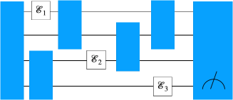
Figure 1: An example of a quantum circuit representing a general $m$-outcome measurement process for $\mathcal{E}_{1}$, $\mathcal{E}_{2}$ and, $\mathcal{E}_{3}$. The channels $\mathcal{E}_{1}$, $\mathcal{E}_{2}$ and, $\mathcal{E}_{3}$ (all the channels to be measured) together are called the input quantum channels, and the blue parts together are called as the quantum tester.

In the quantum tester formalism, quantum channels are represented by Choi operators [35, 36]. A Choi operator $\mathrm{C}_{\mathcal{E}}\in\mathcal{L}(\mathcal{K})\otimes\mathcal{L}(\mathcal{H})$ of a quantum channel $\mathcal{E}:\mathcal{L}(\mathcal{K})\rightarrow\mathcal{L}(\mathcal{H})$ is defined by

$$\mathrm{C}_{\mathcal{E}}:=(id\otimes\mathcal{E})(\ket{\phi^{+}}\bra{\phi^{+}}).$$ (2)

where $\ket{\phi^{+}}:=\sum_{i}\ket{i}\ket{i}$ is a maximally entangled (unnormalized) vector on $\bar{\mathcal{K}}\otimes\mathcal{H}$, and $\bar{\mathcal{K}}$ is a Hilbert space that is isomorphic to the Hilbert space $\mathcal{K}$. In particular, a Choi operator of a unitary operator $U$ is defined as

$$\mathrm{C}_{U}:=(I\otimes U)\ket{\phi^{+}}\bra{\phi^{+}}(I\otimes U^{\dagger})$$ (3)

The Choi operator of the input quantum channels together is given as

$$M=\bigotimes_{k=1}^{n}\mathrm{C}_{\mathcal{E}_{k}}^{\mathcal{K}_{k}\mathcal{H}_{k}},$$ (4)

where we denote the space that the $k$-th Choi operator acts on as $\mathcal{K}_{k}\otimes\mathcal{H}_{k}$.

According to [26, 27], a set of positive semidefinite linear operators $\{\Pi_{1},\ldots,\Pi_{m}\}$ with $\Pi_{i}\in\mathcal{L}(\mathcal{K}_{1}\otimes\mathcal{H}_{1}\otimes\cdots\otimes\mathcal{K}_{n}\otimes\mathcal{H}_{n})$ for all $i$ is a $n$-slot quantum tester with $m$-outcomes for the input quantum channels represented by a Choi operator in $\mathcal{L}(\mathcal{K}_{1}\otimes\mathcal{H}_{1}\otimes\cdots\otimes\mathcal{H}_{n}\otimes\mathcal{H}_{n})$, if there exists a set of linear operator $\{R_{k}\}_{k=1,\ldots,n}$ with $R_{k}\in\mathcal{L}(\mathcal{K}_{1}\otimes\mathcal{H}_{1}\otimes\cdots\otimes\mathcal{K}_{k}\otimes\mathcal{H}_{k})$ that satisfies

$$\sum_{i=1}^{m}\Pi_{i}=R_{n}\otimes I_{\mathcal{H}_{n}}$$ (5)

$$\mathrm{Tr}_{\mathcal{K}_{k}}R_{k}=R_{k-1}\otimes I_{\mathcal{H}_{k-1}}(k=n,\ldots,2)$$ (6)

$$\mathrm{Tr}R_{1}=1.$$ (7)

Fig. 2 shows this quantum tester. We denote input Hilbert spaces as $\mathcal{K}_{i}$ and output Hilbert spaces as $\mathcal{H}_{i}$.

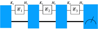
Figure 2: Quantum tester, which is the same as Fig 1, but represented in a simpler form.

The probability of obtaining the outcome $i$ $(i=1,\cdots,m)$ when $M$ is measured is given by

$$\mathrm{Tr}(\Pi_{i}M).$$ (8)

When a quantum tester $\{\Pi_{m}\}$ satisfies $R_{n}\otimes I_{\mathcal{H}_{n}}=S^{\mathcal{K}}\otimes I^{\mathcal{H}}$ for a unit-trace positive semidefinite operator $S^{\mathcal{K}}$ on $\mathcal{K}=\mathcal{K}_{1}\otimes\cdots\otimes\mathcal{K}_{n}$ and an identity operator $I^{\mathcal{H}}$ on $\mathcal{H}=\mathcal{H}_{1}\otimes\cdots\otimes\mathcal{H}_{n}$, the tester is called a parallel tester [27]. By regarding $\mathcal{H}$ and $\mathcal{K}$ as one Hilbert space, the tester can be seen as a 1-slot tester. All input channels $\{\mathcal{E}_{k}\}_{k=1,\ldots,n}$ are used in parallel (Fig.3). The conditions of a parallel tester corresponding to Eq.(5)-(7) are given as

$$\sum_{i=1}^{m}\Pi_{i}=S^{\mathcal{K}}\otimes I^{\mathcal{H}}$$ (9)

$$\mathrm{Tr}S^{\mathcal{K}}=1.$$ (10)

In Eqs. (9) and (10), we use $S$ to denote the single operator representing the condition for a parallel tester to distinguish the case of a general tester in Eq. (2) where a set of operators $\{R_{k}\}_{k=1,\ldots,n}$ is used.

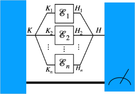
Figure 3: A parallel tester uses $\mathcal{E}_{1}$, …, $\mathcal{E}_{n}$ in parallel. By gathering $\{\mathcal{K}_{i}\}$ and $\{\mathcal{H}_{i}\}$, this tester can be seen as a 1-slot tester.

II.4 Unitary comparison in quantum tester formalism

We apply the quantum tester formalism to unitary comparison. For the comparison task with $N_{1}$ uses of $U_{1}$ and $N_{2}\geq N_{1}$ uses $U_{2}$, we employ a $(N_{1}+N_{2})$-slot quantum tester with two-outcomes “same” or “different” corresponding to Case 1 and Case 2. We denote the elements of such a quantum tester as $\Pi_{1}$, $\Pi_{2}$ for Case 1 and Case 2, respectively, and each element $\Pi_{1}$ is a positive semidefinite operator in $\Pi_{i}\in\mathcal{L}(\mathcal{H}_{1}\otimes\mathcal{K}_{1}\otimes\cdots\otimes\mathcal{H}_{N_{1}+N_{2}}\otimes\mathcal{K}_{N_{1}+N_{2}})$ associated with $\{R_{k}\}_{k=1,\cdots,N_{1}+N_{2}}$ satisfying Eq. (5) to Eq. (7). Since the Choi operator of the total input quantum channels in this task is given by

$$\bigotimes_{k=1}^{N_{1}}\mathrm{C}_{U_{1}}^{\mathcal{K}_{k}\mathcal{H}_{k}}\bigotimes_{k=N_{1}+1}^{N_{1}+N_{2}}\mathrm{C}_{U_{2}}^{\mathcal{K}_{k}\mathcal{H}_{k}},$$

the probability of obtaining outcome $i$ is

$$\mathrm{Tr}(\Pi_{i}\bigotimes_{k=1}^{N_{1}}\mathrm{C}_{U_{1}}^{\mathcal{K}_{k}\mathcal{H}_{k}}\bigotimes_{k=N_{1}+1}^{N_{1}+N_{2}}\mathrm{C}_{U_{2}}^{\mathcal{K}_{k}\mathcal{H}_{k}}).$$

When Case 1 holds, $U_{1}=U_{2}$ and $U_{1}$ is chosen randomly over SU($d$). Then the conditional probability for outcome $i=1$ is obtained by taking the Haar integral of $U_{1}(=U_{2})$ as

$$\begin{split}&\mathrm{Prob}(\text{Outcome $i$=1 when $U_{1}=U_{2}$ })\\ &\qquad=\int dU_{1}\mathrm{Tr}(\Pi_{1}\bigotimes_{k=1}^{N_{1}}\mathrm{C}_{U_{1}}^{\mathcal{K}_{k}\mathcal{H}_{k}}\bigotimes_{k=N_{1}+1}^{N_{1}+N_{2}}\mathrm{C}_{U_{1}}^{\mathcal{K}_{k}\mathcal{H}_{k}})\\ &\qquad=\mathrm{Tr}(\Pi_{1}M_{1}).\end{split}$$ (11)

where

$$M_{1}:=\int dU\bigotimes_{k=1}^{N_{1}+N}\mathrm{C}_{U}^{\mathcal{K}_{k}\mathcal{H}_{k}}$$

represents the averaged Choi operator of the input quantum channels. When Case 2 holds, as both $U_{1}$ and $U_{2}$ are chosen independently randomly over SU($d$), the conditional probability for $i=2$ is obtained as

$$\begin{split}&\mathrm{Prob}(\text{Outcome $i$=2 when $U_{1}\neq U_{2}$ })\\ &=\int dU_{1}dU_{2}\mathrm{Tr}(\Pi_{2}\bigotimes_{k=1}^{N_{1}}\mathrm{C}_{U_{1}}^{\mathcal{K}_{k}\mathcal{H}_{k}}\bigotimes_{k=N_{1}+1}^{N_{1}+N_{2}}\mathrm{C}_{U_{2}}^{\mathcal{K}_{k}\mathcal{H}_{k}})\\ &=\mathrm{Tr}(\Pi_{2}M_{2})\end{split}$$ (12)

where the averaged Choi operator in this case is defined by

$$M_{2}:=\int dU_{1}dU_{2}\bigotimes_{k=1}^{N_{1}}\mathrm{C}_{U_{1}}^{\mathcal{K}_{k}\mathcal{H}_{k}}\bigotimes_{k=N_{1}+1}^{N_{1}+N_{2}}\mathrm{C}_{U_{2}}^{\mathcal{K}_{k}\mathcal{H}_{k}}.$$

Thus, the average success probability is given by

$$\begin{split}&p_{asp}=p\mathrm{Prob}(\text{Outcome $i=1$ when $U_{1}=U_{2}$ })\\ +&(1-p)\mathrm{Prob}(\text{Outcome $i=2$ when $U_{1}\neq U_{2}$ })\\ &=\mathrm{Tr}(p\Pi_{1}M_{1}+(1-p)\Pi_{2}M_{2}).\end{split}$$ (13)

III Optimal comparison in quantum tester formalism when $U_{2}$ is known

III.1 Problem setting

Although unitary comparison aims to compare both unknown unitary channels, we first consider a modified task where $U_{2}$ is perfectly known, but $U_{1}$ is still chosen randomly from SU($d$) in this subsection. In this case, comparison of $U_{1}$ and $U_{2}$ is reduced to an identity check problem of $V:=U_{1}U_{2}^{\dagger}$ without loss of generality, since we can exactly and deterministically apply $U_{2}^{\dagger}$ by utilizing the knowledge of $U_{2}$, whereas exactly and deterministically applying $U_{2}^{\dagger}$ is not possible with finite uses of $U_{2}$ if $U_{2}$ is unknown. More precisely, the task is to discriminate the following two cases

Case 1 $V=I$

$V$ equals to identity operator $I$.

Case 2 $V\neq I$

$V$ is chosen randomly over $\mathrm{SU}(d)$.

by $N_{1}$ uses of $V$.

For the same reason as the original unitary comparison, Case 2 contains the instance of $V=I$ with an infinitely small probability and can be ignored. In this case, the averaged Choi operators subjected to discrimination are

$$M_{1}:=\bigotimes_{k=1}^{N_{1}}\mathrm{C}_{I}^{\mathcal{K}_{k}\mathcal{H}_{k}},$$ (14)

$$M_{2}:=\int dV\bigotimes_{k=1}^{N_{1}}\mathrm{C}_{V}^{\mathcal{K}_{k}\mathcal{H}_{k}}.$$ (15)

III.2 Optimal average success probability

We obtain the following Lemma on the optimal average success probability $p_{asp}:=\mathrm{Tr}(p\Pi_{1}M_{1}+(1-p)\Pi_{2}M_{2})$ of this modified comparison task in the quantum tester formalism.

Lemma 1.

The optimal average success probability of the modified comparison task in the quantum tester formalism when $U_{2}$ is known and $U_{1}$ can be used $N_{1}$ times is

$$p_{asp}=\begin{cases}1-p&(0\leq p\leq\frac{1}{1+\gamma_{N_{1},d}})\\ 1-\frac{1-p}{\gamma_{N_{1},d}}&(\frac{1}{1+\gamma_{N_{1},d}}<p\leq 1),\end{cases}$$ (16)

where $\gamma_{n,d}$ is a binomial coefficient defined by

$$\gamma_{n,d}\coloneqq\begin{pmatrix}n+d^{2}-1\\ n\end{pmatrix}.$$ (17)

Proof.

The averaged Choi operators $M_{1}$ and $M_{2}$ in this case can be transformed to

$$\begin{split}&M_{1}=\bigotimes_{k=1}^{N_{1}}\mathrm{C}_{I}^{\mathcal{K}_{k}\mathcal{H}_{k}}\\ &\qquad=\bigotimes_{k=1}^{N_{1}}\ket{\phi^{+}}\bra{\phi^{+}}^{\mathcal{K}_{k}\mathcal{H}_{k}}\\ &\qquad=\ket{\Phi^{+}}\bra{\Phi^{+}}^{\mathcal{K}\mathcal{H}},\end{split}$$ (18)

and

$$\begin{split}&M_{2}=\int dV\bigotimes_{k=1}^{N_{1}}\mathrm{C}_{V}^{\mathcal{K}_{k}\mathcal{H}_{k}}\\ &\qquad=\int dV\bigotimes_{k=1}^{N_{1}}(I^{\mathcal{K}_{k}}\otimes V^{\mathcal{H}_{k}})\ket{\phi^{+}}\bra{\phi^{+}}^{\mathcal{K}_{k}\mathcal{H}_{k}}\\ &\qquad\qquad(I^{\mathcal{K}_{k}}\otimes V^{\mathcal{H}_{k}})^{\dagger}\\ &\qquad=\int dV(I^{\mathcal{K}}\otimes[V^{\otimes N_{1}}]^{\mathcal{H}})|\Phi^{+}\rangle\langle\Phi^{+}|^{\mathcal{K}\mathcal{H}}\\ &\qquad\qquad(I^{\mathcal{K}}\otimes[V^{\otimes N_{1}}]^{\mathcal{H}})^{\dagger},\end{split}$$ (19)

respectively, where $\ket{\Phi^{+}}^{\mathcal{K}\mathcal{H}}\coloneqq\bigotimes_{k=1}^{N_{1}}\ket{\phi^{+}}^{\mathcal{K}_{k}\mathcal{H}_{k}}$ is a maximally entangled vector on a bipartite Hilbert space $\mathcal{K}\otimes\mathcal{H}$ with $\mathcal{K}\coloneqq\mathcal{K}_{1}\otimes\cdots\otimes\mathcal{K}_{N_{1}}$ and $\mathcal{H}\coloneqq\mathcal{H}_{1}\otimes\cdots\otimes\mathcal{H}_{N_{1}}$.

The Hilbert spaces $\mathcal{K}$ and $\mathcal{H}$ can be decomposed using the Schur-Weyl duality [37, 38, 39] as

$$\mathcal{K}=\bigoplus_{J}\mathcal{U}_{J}^{\mathcal{K}}\otimes\mathcal{V}_{J}^{\mathcal{K}}$$ (20)

$$\mathcal{H}=\bigoplus_{J}\mathcal{U}_{J}^{\mathcal{H}}\otimes\mathcal{V}_{J}^{\mathcal{H}},$$ (21)

where $J$ is a label corresponding to the representation of symmetric group $\mathfrak{S}(N_{1})$, $\mathcal{U}_{J}^{\mathcal{K}}$ ($\mathcal{U}_{J}^{\mathcal{H}}$) is a subspace corresponding to the representation of $U\in\mathrm{SU}(d)$, labeled by $J$, and $\mathcal{V}_{J}^{\mathcal{K}}$ ($\mathcal{V}_{J}^{\mathcal{H}}$) is a subspace corresponding to the representation of $\sigma\in\mathfrak{S}(N_{1})$, labeled by $J$. With this decomposition, we can represent $[U^{\otimes N_{1}}]^{\mathcal{H}}$ as

$$[U^{\otimes N_{1}}]^{\mathcal{H}}=\sum_{J}U_{\mathcal{U}_{J}^{\mathcal{H}}}\otimes I_{\mathcal{V}_{J}^{\mathcal{H}}},$$ (22)

where $U_{\mathcal{U}_{J}^{\mathcal{H}}}$ is a unitary representation on $\mathcal{U}_{J}^{H}$, and $I_{\mathcal{V}_{J}^{\mathcal{H}}}$ is an identity operator on $\mathcal{V}_{J}^{\mathcal{H}}$.

By denoting a maximally entangled vector on the bipartite Hilbert space $\mathcal{U}_{J}^{\mathcal{K}}\otimes\mathcal{U}_{J}^{\mathcal{H}}$ as

$$\ket{\phi^{+}}^{\mathcal{K}\mathcal{H}}_{\mathcal{U}_{J}}\coloneqq\sum_{i=1}^{\dim{\mathcal{U}_{J}}}\ket{i}_{\mathcal{U}_{J}^{\mathcal{K}}}\otimes\ket{i}_{\mathcal{U}_{J}^{\mathcal{H}}}$$ (23)

and a maximally entangled vector on the bipartite Hilbert space $\mathcal{V}_{J}^{\mathcal{K}}\otimes\mathcal{V}_{J}^{\mathcal{H}}$ as

$$\ket{\phi^{+}}^{\mathcal{K}\mathcal{H}}_{\mathcal{V}_{J}}\coloneqq\sum_{i=1}^{\dim{\mathcal{V}_{J}}}\ket{i}_{\mathcal{V}_{J}^{\mathcal{K}}}\otimes\ket{i}_{\mathcal{V}_{J}^{\mathcal{H}}},$$ (24)

the maximally entangled vector $\ket{\Phi^{+}}^{\mathcal{K}\mathcal{H}}$ can be written as

$$\ket{\Phi^{+}}^{\mathcal{K}\mathcal{H}}=\sum_{J}\ket{\phi^{+}}^{\mathcal{K}\mathcal{H}}_{\mathcal{U}_{J}}\otimes\ket{\phi^{+}}^{\mathcal{K}\mathcal{H}}_{\mathcal{V}_{J}}.$$ (25)

By using Eq. (22) and Eq. (25), we obtain an explicit expression of $M_{2}$ as

$$M_{2}=\sum_{J}\frac{I^{\mathcal{K}}_{\mathcal{U}_{J}}\otimes I^{\mathcal{H}}_{\mathcal{U}_{J}}}{\dim{\mathcal{U}_{J}}}\otimes\ket{\phi^{+}}\bra{\phi^{+}}^{\mathcal{K}\mathcal{H}}_{\mathcal{V}_{J}},$$ (26)

as proven in Appendix B. The value $\sum_{J}(\dim\mathcal{U}_{J})^{2}$ can be explicitly given [37, 30] as

$$\gamma_{N_{1},d}\coloneqq\sum_{J}(\dim\mathcal{U}_{J})^{2}=\begin{pmatrix}N_{1}+d^{2}-1\\ N_{1}\end{pmatrix}.$$ (27)

Achievability

We show that there exists a strategy that provides the average success probability $p_{asp}$ given by Eq. (16), and we further show that the average success probability $p_{asp}$ given by Eq. (16) achieves the upper bound in the given condition. As the optimal strategy depends on the range of $p$, we present the following two cases separately.

(i) For the case of $0\leq p\leq\frac{1}{1+\gamma_{N_{1},d}}$:

The strategy is to conclude $U_{1}\neq U_{2}$ without applying the quantum tester. The average success probability $p_{asp}$ is given as

$$\begin{split}&p_{asp}=p\mathrm{Prob}(\text{Outcome $i=1$ when $U_{1}=U_{2}$})\\ &+(1-p)\mathrm{Prob}(\text{Outcome $i=2$ when $U_{1}\neq U_{2}$})\\ &=p\cdot 0+(1-p)\cdot 1=1-p\end{split}$$ (28)

(ii) For the case of $\frac{1}{1+\gamma_{N_{1},d}}<p\leq 1$:

Let us define a parallel tester $S$ and $\{\Pi_{i}\}$ given by

$$S^{\mathcal{K}}=\sum_{J}q_{J}\frac{I_{\mathcal{U}_{J}^{\mathcal{K}}}}{\dim\mathcal{U}_{J}}\otimes\frac{I_{\mathcal{V}_{J}^{\mathcal{K}}}}{\dim\mathcal{V}_{J}}$$ (29)

$$\Pi_{1}=S^{\mathcal{K}}\otimes I^{\mathcal{H}}\ket{\Phi^{+}}\bra{\Phi^{+}}^{\mathcal{K}\mathcal{H}}S^{\mathcal{K}}\otimes I^{\mathcal{H}}$$ (30)

$$\Pi_{2}=S^{\mathcal{K}}\otimes I^{\mathcal{H}}-\Pi_{1},$$ (31)

where $q_{J}$ is set to be

$$q_{J}=\frac{(\dim\mathcal{U}_{J})^{2}}{\sum_{J}(\dim\mathcal{U}_{J})^{2}}.$$ (32)

Since $S{{}^{\mathcal{K}}}$ and $\ket{\Phi^{+}}\bra{\Phi^{+}}^{\mathcal{K}\mathcal{H}}$ are positive semidefinite, $\Pi_{1}$ is positive semidefinite. By defining a state $\ket{\psi}^{\mathcal{K}\mathcal{H}}\coloneqq\sqrt{S}^{\mathcal{K}}\otimes I^{\mathcal{H}}\ket{\Phi^{+}}^{\mathcal{K}\mathcal{H}}$ satisfying $\braket{\psi}{\psi}=\mathrm{Tr}S^{\mathcal{K}}=1$, $\Pi_{2}$ is shown to be positive semidefinite as

$$\begin{split}\Pi_{2}&=S^{\mathcal{K}}\otimes I^{\mathcal{H}}-\Pi_{1}\\ &=\sqrt{S}^{\mathcal{K}}\otimes I^{\mathcal{H}}(I^{\mathcal{K}}\otimes I^{\mathcal{H}}-{\ket{\psi}}\bra{\psi}^{\mathcal{K}\mathcal{H}})\sqrt{S}^{\mathcal{K}}\otimes I^{\mathcal{H}}\\ &\geq 0,\end{split}$$ (33)

where the last inequality is due to the fact that $I\geq\rho$ holds for any density operator $\rho$. Due to $\Pi_{1}+\Pi_{2}=S{{}^{\mathcal{K}}}\otimes I^{\mathcal{H}}$ and $\mathrm{Tr}S^{\mathcal{K}}=1$, the parallel tester conditions Eq. (9) and Eq. (10) are satisfied, thus we can conclude $\{\Pi_{i}\}$ is a valid set of positive semidefinite linear operators describing a quantum tester.

Inserting Eq. (29) in Eq (30), we have

$$\begin{split}\Pi_{1}=&\sum_{J_{1}J_{2}}\frac{q_{J_{1}}q_{J_{2}}}{\dim\mathcal{U}_{J_{1}}\dim\mathcal{V}_{J_{1}}\dim\mathcal{U}_{J_{2}}\dim\mathcal{V}_{J_{2}}}\\ &\quad\cdot\ket{\phi^{+}}\bra{\phi^{+}}^{\mathcal{K}\mathcal{H}}_{\mathcal{U}_{J_{2}}}\otimes\ket{\phi^{+}}\bra{\phi^{+}}^{\mathcal{K}\mathcal{H}}_{\mathcal{V}_{J_{2}}}.\end{split}$$ (34)

Using Eq. (34), following probabilities can be calculated as

$$\begin{split}\mathrm{Tr}(\Pi_{1}M_{2})=&\sum_{JJ_{1}J_{2}}\frac{q_{J_{1}}q_{J_{2}}}{\dim\mathcal{U}_{J}\dim\mathcal{U}_{J_{1}}\dim\mathcal{V}_{J_{1}}\dim\mathcal{U}_{J_{2}}\dim\mathcal{V}_{J_{2}}}\\ &\cdot{\bra{\phi^{+}}^{\mathcal{K}\mathcal{H}}_{\mathcal{U}_{J_{2}}}\ket{\phi^{+}}\bra{\phi^{+}}^{\mathcal{K}\mathcal{H}}_{\mathcal{V}_{J_{2}}}\ket{\phi^{+}}\bra{\phi^{+}}^{\mathcal{K}\mathcal{H}}_{\mathcal{V}_{J}}\ket{\phi^{+}}^{\mathcal{K}\mathcal{H}}_{\mathcal{V}_{J_{1}}}}\\ =&\sum_{J}\frac{q_{J}^{2}}{(\dim\mathcal{U}_{J})^{2}}=\frac{1}{\sum_{J}(\dim\mathcal{U}_{J})^{2}},\end{split}$$ (35)

$$\begin{split}\mathrm{Tr}(\Pi_{1}M_{1})&=(\bra{\Phi^{+}}^{\mathcal{K}\mathcal{H}}S^{\mathcal{K}}\otimes I^{\mathcal{H}}\ket{\Phi^{+}}^{\mathcal{K}\mathcal{H}})^{2}\\ &=(\mathrm{Tr}S)^{2}=1,\end{split}$$ (36)

and thus

$$\begin{split}&\mathrm{Tr}(\Pi_{2}M_{2})=\mathrm{Tr}((S\otimes I)M_{2})-\mathrm{Tr}(\Pi_{1}M_{2})\\ &=1-\frac{1}{\sum_{J}(\dim\mathcal{U}_{J})^{2}}.\end{split}$$ (37)

Therefore, the average success probability is calculated as

$$\begin{split}p_{asp}&=\mathrm{Tr}(pM_{1}\Pi_{1}+(1-p)M_{2}\Pi_{2})\\ &=p+(1-p)\left(1-\frac{1}{\sum_{J}(\dim\mathcal{U}_{J})^{2}}\right)\\ &=1-\frac{1-p}{\sum_{J}(\dim\mathcal{U}_{J})^{2}}\\ &=1-\frac{1-p}{\gamma_{N_{1},\>d}}.\end{split}$$ (38)

A parallel tester for identity check of $V$ with $N_{1}$ uses can be implemented by the following preparation-measurement process:

• Preparation of $\ket{\psi}^{\mathcal{K}\mathcal{H}}\coloneqq\sqrt{S}^{\mathcal{K}}\otimes I^{\mathcal{H}}\ket{\Phi^{+}}^{\mathcal{K}\mathcal{H}}$,

• Applying $V$ in parallel, namely, $[V^{\otimes N_{1}}]^{\mathcal{H}}$ to $\ket{\psi}^{\mathcal{K}\mathcal{H}}$,

• Measurement of the final state $(I^{\mathcal{K}}\otimes[V^{\otimes N_{1}}]^{\mathcal{H}})\ket{\psi}\bra{\psi}^{\mathcal{K}\mathcal{H}}(I^{\mathcal{K}}\otimes[V^{\otimes N_{1}}]^{\mathcal{H}})^{\dagger}$ by a POVM $\left\{\tilde{\Pi}_{i}=([\sqrt{S}^{-1}]^{\mathcal{K}}\otimes I^{\mathcal{H}})\Pi_{i}([\sqrt{S}^{-1}]^{\mathcal{K}}\otimes I^{\mathcal{H}})\right\}_{i=1,2}$.

A quantum circuit representing this preparation-measurement process is shown in Fig. 4.

The equivalence of the quantum tester and the process (i)–(iii) can be seen as follows. The state just before the POVM in step (iii) is given as $\rho_{i}=\sqrt{S}^{\mathcal{K}}\otimes I^{\mathcal{H}}M_{i}\sqrt{S}^{\mathcal{K}}\otimes I^{\mathcal{H}}$ for Case $i$ ($i=1,2$). The average success probability of this process is given by

$$\begin{split}p_{asp}&:=\mathrm{Tr}(p\rho_{1}\tilde{\Pi}_{1}+(1-p)\rho_{2}\tilde{\Pi}_{2})\\ &=\mathrm{Tr}(p\sqrt{S}^{\mathcal{K}}\otimes I^{\mathcal{H}}M_{1}\sqrt{S}^{\mathcal{K}}\otimes I^{\mathcal{H}})\\ &([\sqrt{S}^{-1}]^{\mathcal{K}}\otimes I^{\mathcal{H}})\Pi_{1}([\sqrt{S}^{-1}]^{\mathcal{K}}\otimes I^{\mathcal{H}}))\\ +&\mathrm{Tr}((1-p)\sqrt{S}^{\mathcal{K}}\otimes I^{\mathcal{H}}M_{2}\sqrt{S}^{\mathcal{K}}\otimes I^{\mathcal{H}}\\ &([\sqrt{S}^{-1}]^{\mathcal{K}}\otimes I^{\mathcal{H}})\Pi_{2}([\sqrt{S}^{-1}]^{\mathcal{K}}\otimes I^{\mathcal{H}}))\\ &=\mathrm{Tr}(pM_{1}\Pi_{1}+(1-p)M_{2}\Pi_{2}).\end{split}$$ (39)

Thus, the process given by (i) – (iii) implement the parallel tester $\{\Pi_{1},\Pi_{2}\}$ in the sense of achieving the average success probability.

Figure 4: Quantum circuit of the optimal strategy of identity check of $V$. All input quantum channels are used in parallel.

Optimality

We show that this strategy is optimal in the sense of the average success probability. The optimization problem of this unitary comparison with a general tester is formularized as the semidefinite programming [40] given by

$$\mathrm{maximize:}p_{asp}\coloneqq\mathrm{Tr}(pM_{1}\Pi_{1}+(1-p)M_{2}\Pi_{2})$$ (40)

$$\Pi_{1},\Pi_{2}\in\mathcal{L}(\bigotimes_{k=1}^{n}(\mathcal{K}_{k}\otimes\mathcal{H}_{k})$$ (41)

$$\Pi_{1},\Pi_{2}\geq 0$$ (42)

$$R_{i}\in\mathcal{L}((\bigotimes_{k=1}^{i}(\mathcal{K}_{k}\otimes\mathcal{H}_{k})\otimes\mathcal{K}_{i+1})\qquad(i=1,\ldots,n)$$ (43)

$$R_{1}\in\mathcal{L}(\mathcal{K}_{1})$$ (44)

$$\Pi_{1}+\Pi_{2}=R_{n}\otimes I^{\mathcal{H}_{n}}$$ (45)

$$R_{i}\geq 0\qquad(i=1,\ldots,n)$$ (46)

$$\mathrm{Tr}_{\mathcal{K}_{i}}R_{i}=R_{i-1}\otimes I^{\mathcal{H}_{i-1}}\qquad(i=2,\ldots,n)$$ (47)

$$\mathrm{Tr}R_{1}=1.$$ (48)

As shown in Appendix A, a parameter $\lambda$ of the following dual SDP problem gives the upper bound of $p_{asp}$,

$$\mathrm{minimize:}\lambda\in\mathbb{R}$$ (49)

$$\Omega_{k}\in\mathcal{L}(\bigotimes_{l=1}^{i}(\mathcal{K}_{l}\otimes\mathcal{H}_{l}))\qquad(k=1,\ldots,N_{1})$$ (50)

$$\Omega_{k}\geq 0$$ (51)

$$pM_{1}-\Omega_{N_{1}}\leq 0$$ (52)

$$(1-p)M_{2}-\Omega_{N_{1}}\leq 0$$ (53)

$$\mathrm{Tr}_{\mathcal{H}_{k}}\Omega_{k}-\Omega_{k-1}\otimes I^{\mathcal{K}_{k}}\leq 0\qquad(k=2,\ldots,N_{1})$$ (54)

$$\mathrm{Tr}_{\mathcal{H}_{1}}\Omega_{1}-\lambda I^{\mathcal{K}_{1}}\leq 0.$$ (55)

Let us define the Choi operators of the input channels to be

$$M_{1}^{(k)}=\bigotimes_{l=1}^{k}\mathrm{C}_{I}^{\mathcal{K}_{l}\mathcal{H}_{l}},$$ (56)

$$M_{2}^{(k)}=\int dV\bigotimes_{l=1}^{k}\mathrm{C}_{V}^{\mathcal{K}_{l}\mathcal{H}_{l}}$$ (57)

for $k=1,\ldots,N_{1}$. Note that we have

$$\begin{split}\mathrm{Tr}_{\mathcal{H}_{k}}M_{1}^{(k)}&=M_{1}^{(k-1)}\otimes\mathrm{Tr}_{\mathcal{H}_{k}}(\ket{\phi^{+}}\bra{\phi^{+}}^{\mathcal{K}_{k}\mathcal{H}_{k}})\\ &=M_{1}^{(k-1)}\otimes I^{\mathcal{K}_{k}},\end{split}$$ (58)

and

$$\begin{split}\mathrm{Tr}_{\mathcal{H}_{k}}M_{2}^{(k)}&=\int dV\bigotimes_{l=1}^{k-1}\mathrm{C}_{V}^{\mathcal{K}_{l}\mathcal{H}_{l}}\otimes\mathrm{Tr}_{\mathcal{H}_{k}}(\mathrm{C}_{V}^{\mathcal{K}_{k}\mathcal{H}_{k}})\\ &=\int dV\bigotimes_{l=1}^{k-1}\mathrm{C}_{V}^{\mathcal{K}_{l}\mathcal{H}_{l}}\otimes\mathrm{Tr}_{\mathcal{H}_{k}}(I^{\mathcal{K}_{k}}\\ &\otimes V\ket{\phi^{+}}\bra{\phi^{+}}^{\mathcal{K}_{k}\mathcal{H}_{k}}I^{\mathcal{K}_{k}}\otimes V^{\dagger})\\ &=\int dV\bigotimes_{l=1}^{k-1}\mathrm{C}_{V}^{\mathcal{K}_{l}\mathcal{H}_{l}}\otimes I^{\mathcal{K}_{k}}\\ &=M_{2}^{(k-1)}\otimes I^{\mathcal{K}_{k}}\end{split}$$ (59)

for $k=2,\ldots,N_{1}$.

(i) For the case of $0\leq p\leq\frac{1}{1+\gamma_{N_{1},d}}$:

Let us define $\Omega_{k}$ and $\lambda$ as

$$\Omega_{k}=(1-p)M_{2}^{(k)}\qquad(k=1,\ldots,N_{1}),$$ (60)

$$\lambda=1-p.$$ (61)

Apparently, $\Omega_{k}\geq 0$ for $k=1,\ldots,N_{1}$, $\mathrm{Tr}_{\mathcal{H}_{k}}\Omega_{k}-\Omega_{k-1}\otimes I^{\mathcal{K}_{k}}=0$ for $k=2,\ldots,N_{1}$, $\mathrm{Tr}_{\mathcal{H}_{1}}\Omega_{1}-\lambda I^{\mathcal{K}_{1}}=0$, and $(1-p)M_{2}-\Omega_{N_{1}}=0$. Moreover, we have

$$\begin{split}&pM_{1}-\Omega_{N_{1}}\leq 0\\ &\iff pM_{1}\leq(1-p)M_{2},\end{split}$$ (62)

and this follows from the relation

$$pM_{1}\leq\frac{1-p}{\gamma_{N_{1},\>d}}M_{1}\leq(1-p)M_{2}$$ (63)

where we used the relation

$$p\leq\frac{1}{1+\gamma_{N_{1},\>d}}\leq\frac{1-p}{\gamma_{N_{1},\>d}},$$ (64)

and the inequality $M_{1}/\gamma_{N_{1},\>d}\leq M_{2}$ (144). Thus, the set $\{\lambda,\Omega_{k}\}$ are a valid solution of Eq. (49) – Eq. (55) for $0\leq p\leq\frac{1}{1+\gamma_{N_{1},d}}$.

(i) For the case of $0\leq p\leq\frac{1}{1+\gamma_{N_{1},d}}$:

Let us define $\Omega_{k}$ and $\lambda$ as

$$\begin{split}\Omega_{k}&=\left(p-\frac{1-p}{\gamma_{N_{1},\>d}}\right)M_{1}^{(k)}\\ &\qquad+(1-p)M_{2}^{(k)}\qquad(k=1,\ldots,N_{1})\\ \lambda&=1-\frac{1-p}{\gamma_{N_{1},\>d}}.\end{split}$$ (65)

Note that the first term of $\Omega_{k}$ is positive since

$$p-\frac{1-p}{\gamma_{N_{1},\>d}}=\frac{p(\gamma_{N_{1},\>d}+1)-1}{\gamma_{N_{1},\>d}}>0.$$ (66)

Apparently, $\Omega_{k}\geq 0$ ($k=1,\ldots,N_{1}$), $\mathrm{Tr}_{\mathcal{H}_{i}}\Omega_{i}-\Omega_{i-1}\otimes I^{\mathcal{K}_{i}}=0$ ($i=2,\ldots,N_{1}$) $\mathrm{Tr}_{\mathcal{H}_{1}}\Omega_{1}-\lambda I^{\mathcal{K}_{1}}=0$, and $(1-p)M_{2}-\Omega_{N_{1}}\leq 0$ hold. Moreover, we have

$$\begin{split}&pM_{1}-\Omega_{N_{1}}\leq 0\\ &\iff pM_{1}\leq\left(p-\frac{1-p}{\gamma_{N_{1},d}}\right)M_{1}+(1-p)M_{2}\\ &\iff 0\leq-\frac{1-p}{\gamma_{N_{1},d}}M_{1}+(1-p)M_{2}\\ &\iff\frac{1}{\gamma_{N_{1},d}}M_{1}\leq M_{2}.\end{split}$$ (67)

where we used the relation shown in $M_{1}/\gamma_{N_{1},\>d}\leq M_{2}$ (144) of Appendix B in the last inequality. Thus, these $\{\lambda,\Omega_{k}\}$ are a valid solution of Eq. (49) – Eq. (55) when $\frac{1}{1+\gamma_{N_{1},\>d}}<p\leq 1$ holds. Now, the dual SDP solution above asserts the optimality of $p_{asp}$. ∎

IV The optimal comparison when $U_{2}$ is unknown

IV.1 The optimal comparison in quantum tester formalism when $N_{1}$ uses of $U_{2}^{*}$ is available

First, we show that if $N_{1}$ uses of $U_{2}^{*}$ (complex conjugate of $U_{2}$) is available, we can achieve the same optimal average success probability $p_{asp}$ in the quantum tester formalism as the case of $U_{2}$ is known, even though $U_{2}$ is unknown.

Lemma 2.

When both $U_{1}$ and $U_{2}^{*}$ can be used $N_{1}$ times, we can achieve the same optimal average success probability $p_{asp}$ in the quantum tester formalism as the case of $U_{2}$ is known, namely,

$$p_{asp}=\begin{cases}1-p&(0\leq p\leq\frac{1}{1+\gamma_{N_{1},d}})\\ 1-\frac{1-p}{\gamma_{N_{1},d}}&(\frac{1}{1+\gamma_{N_{1},d}}<p\leq 1).\end{cases}$$ (68)

Proof.

Using the irreducible decompositions representations of $U^{\otimes N_{1}}$ given by Eq. (22), $S^{\mathcal{K}}$ given by Eq. (29) can be shown to commute with $U^{\otimes N_{1}}$ for arbitrary unitary $U$ as

$$\begin{split}&[S^{\mathcal{K}},\>U^{\otimes N_{1}}]\\ &\qquad=\sum_{J,J^{\prime}}\left[q_{J}\frac{I_{\mathcal{U}_{J}^{\mathcal{K}}}}{\dim\mathcal{U}_{J}}\otimes\frac{I_{\mathcal{V}_{J}^{\mathcal{K}}}}{\dim\mathcal{V}_{J}},\>U_{\mathcal{U}_{J^{\prime}}^{\mathcal{K}}}\otimes I_{\mathcal{V}_{J^{\prime}}^{\mathcal{K}}}\right]\\ &\qquad=0.\end{split}$$ (69)

The optimal comparison strategy when $U_{2}$ is known can be written as three steps by replacing $V$ in the preparation-measurement process presented in the previous section by $V=U_{1}U_{2}^{\dagger}$ as

• Preparation of the initial state $\ket{\psi}\coloneqq\sqrt{S}^{\mathcal{K}}\otimes I^{\mathcal{H}}\ket{\Phi^{+}}^{\mathcal{K}\mathcal{H}}$

• Applying $(U_{1}U_{2}^{\dagger})^{\otimes N_{1}}$ to the subsystem $\mathcal{H}$ of $\ket{\psi}$

• Performing a measurement using a POVM given by $\{\tilde{\Pi}_{i}=([\sqrt{S}^{-1}]^{\mathcal{K}}\otimes I^{\mathcal{H}})\Pi_{i}([\sqrt{S}^{-1}]^{\mathcal{K}}\otimes I^{\mathcal{H}})\}_{i=1,2}$ where $\Pi_{1}$, $\Pi_{2}$ are defined by Eq. (30) and Eq. (31)

Note that as long as $U_{2}^{\dagger}$ can be applicable $N_{1}$ times, this strategy works. Thus we do not need to know about $U_{2}^{\dagger}$ itself to perform this strategy if $U_{2}^{\dagger}$ is provided. The strategy consisting of the three steps is represented by a quantum circuit shown in Fig. 5.

We can rewrite the quantum circuit given by Fig. 5 into the one with $U_{1}$ and $U_{2}^{*}$ as shown in Fig. 6. Due to the property of the maximally entangle vector $I\otimes AB\ket{\phi^{+}}=B^{T}\otimes A\ket{\phi^{+}}$, and the commutability of $S$ and $U^{\otimes N_{1}}$,

$$\begin{split}&I^{\mathcal{K}}\otimes(U_{1}U_{2}^{\dagger})^{\otimes N_{1}}\ket{\psi}\\ &\qquad=\sqrt{S}^{\mathcal{K}}\otimes(U_{1}U_{2}^{\dagger})^{\otimes N_{1}}\ket{\Phi^{+}}\\ &\qquad=\sqrt{S}^{\mathcal{K}}\otimes I^{\mathcal{H}}(I\otimes U_{1}U_{2}^{\dagger}\ket{\phi^{+}})^{\otimes N_{1}}\\ &\qquad=\sqrt{S}^{\mathcal{K}}\otimes I^{\mathcal{H}}(U_{2}^{*}\otimes U_{1}\ket{\phi^{+}})^{\otimes N_{1}}\\ &\qquad=\sqrt{S}^{\mathcal{K}}U_{2}^{*\otimes N_{1}}\otimes U_{1}^{\otimes N_{1}}\ket{\Phi^{+}}\\ &\qquad=U_{2}^{*\otimes N_{1}}\sqrt{S}^{\mathcal{K}}\otimes U_{1}^{\otimes N_{1}}\ket{\Phi^{+}}\\ &\qquad=U_{2}^{*\otimes N_{1}}\otimes U_{1}^{\otimes N_{1}}\ket{\psi}.\end{split}$$ (70)

Thus, when both $U_{1}$ and $U_{2}^{*}$ can be used $N_{1}$ times, we can achieve the same average success probability $p_{asp}$ by the strategy given by

• Preparation of the initial state $\ket{\psi}\coloneqq\sqrt{S}^{\mathcal{K}}\otimes I^{\mathcal{H}}\ket{\Phi^{+}}^{\mathcal{K}\mathcal{H}}$

• Applying $U_{1}^{\otimes N_{1}}$ to the subsystem $\mathcal{H}$ of $\ket{\psi}$ and applying $U_{2}^{*\otimes N_{1}}$ to the subsystem $\mathcal{K}$ of $\ket{\psi}$.

• Performing a measurement using a POVM given by $\{\tilde{\Pi}_{i}=([\sqrt{S}^{-1}]^{\mathcal{K}}\otimes I^{\mathcal{H}})\Pi_{i}([\sqrt{S}^{-1}]^{\mathcal{K}}\otimes I^{\mathcal{H}})\}_{i=1,2}$ where $\Pi_{1}$, $\Pi_{2}$ are defined by Eq. (30) and Eq. (31)

Figure 5: Quantum circuit representation of the optimal comparison strategy when both $U_{1}$ and $U_{2}^{\dagger}$ can be used $N_{1}$ times.

Figure 6: Quantum circuit representation of the comparison strategy when both $U_{1}$ and $U_{2}^{*}$ can be used $N_{1}$ times.

∎

IV.2 The optimal comparison in quantum tester formalism when $N_{2}$ uses of unknown $U_{2}$ is available

If the action of $U_{2}^{*}$ can be applied by using unknown $U_{2}$ finite times, the optimal average success probability of unitary comparison with known $U_{2}$ is achievable. Such a task of transforming an unknown unitary channel $U$ to its complex conjugate channel $U^{*}$ by using $U$ multiple times is known as unitary complex conjugation presented in [41].

Proposition 1.

(Conjugate algorithm [41]) There exists an algorithm to deterministically transform $U$ to $U^{*}$ by $d-1$ uses of $U$ in parallel.

Using this proposition, we conclude the following Theorem.

Theorem 1.

The optimal average success probability $p_{asp}$ of the comparison of $U_{1}$ and $U_{2}$ with $N_{1}$ uses of $U_{1}$ and $N_{2}\geq N_{1}(d-1)$ uses of $U_{2}$ in the quantum tester formalism is given by

$$p_{asp}=\begin{cases}1-p&(0\leq p\leq\frac{1}{1+\gamma_{N_{1},d}})\\ 1-\frac{1-p}{\gamma_{N_{1},d}}&(\frac{1}{1+\gamma_{N_{1},d}}<p\leq 1),\end{cases}$$ (71)

where $\gamma_{N_{1},d}$ is given by

$$\gamma_{N_{1},d}\coloneqq\begin{pmatrix}N_{1}+d^{2}-1\\ N_{1}\end{pmatrix}.$$ (72)

Proof.

For the case of $N_{2}\geq N_{1}(d-1)$, $N_{2}=N_{1}(d-1)$ uses of $U_{2}$ can implement the action of $N_{1}$ uses of $U_{2}^{*}$ by Proposition 1. Then $N_{1}$ uses of $U_{1}$ and $N_{1}(d-1)$ uses of $U_{2}$ can achieves the optimal average success probability

$$p_{asp}=\begin{cases}1-p&(0\leq p\leq\frac{1}{1+\gamma_{N_{1},d}})\\ 1-\frac{1-p}{\gamma_{N_{1},d}}&(\frac{1}{1+\gamma_{N_{1},d}}<p\leq 1)\end{cases}$$ (73)

by Lemma 2. This optimal average success probability in the quantum tester formalism is identical to the case of the optimal $p_{asp}$ when $N_{1}$ uses of $U_{1}$ are possible and $U_{2}$ is known.

We cannot improve the average success probability $p_{asp}$ by the remaining $N_{2}-N_{1}(d-1)$ uses of $U_{2}$ because the probability cannot be greater than the case of $U_{2}$ is known. To see this, let $\mathcal{B}(N_{2})$ denote the set of strategies that uses $U_{2}$ for $N_{2}$ times, and let $\mathcal{B}_{known}$ denote the set of strategies when $U_{2}$ is known. By using the knowledge of $U_{2}$, we can implement $U_{2}$ as many times as we want, hence $\mathcal{B}(N_{2})\subset\mathcal{B}_{known}$ holds. The optimal average success probability when $N_{2}$ times uses of $U_{2}$, $p_{asp}(N_{2})$ is bounded by

$$p_{asp}(N_{2}) =\sup_{s\in\mathcal{B}(N_{2})}p_{asp}(s)$$ (74)

$$\leq\sup_{s\in\mathcal{B}_{known}}p_{asp}(s)=:p_{asp}^{known},$$ (75)

where $p_{asp}^{known}$ is the optimal average success probability when $U_{2}$ is known. Noting that

$$p_{asp}(N_{1}(d-1))\leq p_{asp}(N_{2})\leq p_{asp}^{known}$$ (76)

for $N_{2}\geq N_{1}(d-1)$, and $p_{asp}(N_{1}(d-1))=p_{asp}^{known}$ from Lemma 2, we conclude that $p_{asp}(N_{2})=p_{asp}^{known}$ for $N_{1}(d-1)\leq N_{2}$. ∎

As appeared in the proof, one notable property of the minimum-error optimal average probability $p_{asp}$ given by Eq. (71) in Theorem 2 is that when the number of the uses of the channel $N_{1}$ is fixed, $p_{asp}$ is saturated at $N_{2}=(d-1)N_{1}$ and it cannot be improved by adding more uses of $U_{2}$. This was due to the fact that the same $p_{asp}$ to the one for the case of known $U_{2}$ is achieved by finite (i.e. $N_{2}=(d-1)N_{1}$) uses.

In contrast, in quantum state comparison of (unknown) pure states $\ket{\psi_{1}}$ and $\ket{\psi_{2}}$ when $N_{1}$ and $N_{2}\geq N_{1}$ copies are given, respectively, $p_{asp}$ of minimum-error state comparison for a fixed number of $N_{1}$ can be improved by adding more copies of $\ket{\psi_{2}}$. That is, it is not possible to achieve $p_{asp}$ for known $\ket{\psi_{2}}$ by using only finite copies of $\ket{\psi_{2}}$. To see this, we obtain the optimal average success probability of minimum-error state comparison of $\ket{\psi_{1}}$ with $N_{1}$ copies and $\ket{\psi_{2}}$ with $N_{2}$ copies as

$$p_{asp}=\begin{cases}1-p&(0\leq p\leq\frac{1}{1+\beta_{N_{1},N_{2},d}})\\ 1-\frac{1-p}{\beta_{N_{1},N_{2},d}}&(\frac{1}{1+\beta_{N_{1},N_{2},d}}<p\leq 1)\end{cases}$$ (77)

where $\beta_{N_{1},N_{2},d}:=d^{sym}_{N_{1}}d^{sym}_{N_{2}}/d^{sym}_{N_{1}+N_{2}}$ and

$$d^{sym}_{N}:=\begin{pmatrix}N+d-1\\ d-1\end{pmatrix}$$

is the dimension of the symmetric subspace of a $N$-qudit system. The derivation of optimal $p_{asp}$ is shown in Appendix C. The forms of $p_{asp}$ for unitary comparison and pure-state comparison are similar, the difference appears only in the factor $\beta_{N_{1},N_{2},d}$ and $\gamma_{\min(N_{1},N_{2}),d}$. We plot the optimal average success probability of unitary comparison $1-(1-p)/\gamma_{\min(N_{1},N_{2}),d}$ and that of pure-state comparison $1-(1-p)/\beta_{N_{1},N_{2},d}$ for $N_{1}=3$, $d=2$ and $p=1/2$ in Fig. 7. Note that the condition $N_{2}\geq(d-1)N_{1}$ is always satisfied for $d=2$ in our setting of $N_{2}\geq N_{1}$.

Eq. (77) indicates that $p_{asp}$ increases as $N_{2}$ increases and asymptotically approaching $1-(1-p)/d^{sym}_{N_{1}}$ for $N_{2}\rightarrow\infty$ due to the property of $1/\beta_{N_{1},N_{2},d}$. Therefore, when $N_{2}$ is finite, it is not possible to achieve $1-(1-p)/d^{sym}_{N_{1}}$ that is achievable if $\ket{\psi_{2}}$ is known. This fact for the comparison task presents another instance of the different characteristic behaviors of similar tasks for unitary channels and pure states, in addition to the one found for the discrimination tasks for unitary channels and pure states [4, 42, 43].

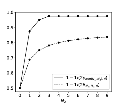
Figure 7: The average success probability of unitary comparison $1-(1-p)/\gamma_{\min(N_{1},N_{2}),d}$ and that of state comparison $1-(1-p)/\beta_{N_{1},N_{2},d}$ are plotted for $N_{1}=3$, $d=2$ and $p=1/2$. The average success probability of unitary comparison $1-(1-p)/\gamma_{\min(N_{1},N_{2}),d}$ remains the same value for $N_{2}\geq 3$.

IV.3 Extension to quantum circuits with classical control of causal order

A strategy with classical control of causal order represented by a quantum circuit with control of causal order (QC-CC) [34] describes a strategy where the causal order of the use of the channels is determined adaptively based on a measurement applied during the protocol. This class of strategies is strictly larger than the class of strategies described by the quantum tester formalism but still implementable in the quantum circuit model if we allow adoptive changes of causal order depending on measurement outcomes during the protocol. There is a possibility that the optimal success probability may be improved by extending to the class of strategies with classical control of causal order for general tasks. However, such an extension cannot improve the optimal success probability of unitary compassion in the quantum tester formalism.

To see this, recall that when $U_{2}$ is known, the unitary comparison task is reduced to a task concerning a single unknown input channel $U_{1}U_{2}^{\dagger}$. When the same quantum channels are inserted into all input slots in QC-CC, any adoptive change of causal order can be represented by the same fixed causal order, therefore, it can be represented by a quantum tester. When $U_{2}$ is unknown and $N_{2}=(d-1)N_{1}$ is satisfied, we have shown the construction of a parallel tester that can achieve the same optimal average success probability $p_{asp}$ for the case of $U_{2}$ is known. We have also shown that $p_{asp}$ for finite uses of unknown $U_{2}$ cannot be better than $p_{asp}$ for known $U_{2}$ in general, thus the constructed parallel tester is optimal even for the strategy with QC-CC. Therefore, QC-CC does not improve the optimal success probability of unitary comparison for $N_{2}\geq(d-1)N_{1}$, and we obtain the following theorem.

Theorem 2.

The optimal average success probability $p_{asp}$ of the comparison of $U_{1}$ and $U_{2}$ with $N_{1}$ uses of $U_{1}$ and $N_{2}\geq N_{1}(d-1)$ uses of $U_{2}$ in the quantum circuit model with classical control of causal order (QC-CC) is given by

$$p_{asp}=\begin{cases}1-p&(0\leq p\leq\frac{1}{1+\gamma_{N_{1},d}})\\ 1-\frac{1-p}{\gamma_{N_{1},d}}&(\frac{1}{1+\gamma_{N_{1},d}}<p\leq 1),\end{cases}$$ (78)

where $\gamma_{N_{1},d}$ is given by

$$\gamma_{N_{1},d}\coloneqq\begin{pmatrix}N_{1}+d^{2}-1\\ N_{1}\end{pmatrix}.$$ (79)

IV.4 Examples of optimal unitary comparison strategies

We construct concrete strategies of the unitary comparison for the case of the qubit ($d=2$).

• $N_{1}=N_{2}=1$ case: Since $\mathcal{S}^{\mathcal{K}}=I/2$ holds, the initial state $\ket{\psi}$ is a maximally entangled state, and the POVM operators are given by $\Pi_{1}=\ket{\psi}\bra{\psi}$ and $\Pi_{2}=I-\ket{\psi}\bra{\psi}$.

• $N_{1}=N_{2}=2$ case: We decompose a two-qubit Hilbert space into the singlet and triplet subspaces represented by the following orthonormal basis states,

  $$\ket{\omega_{0}}:=\frac{1}{\sqrt{2}}(\ket{01}-\ket{10})$$ (80)

  $$\ket{\omega_{1}}:=\ket{00}$$ (81)

  $$\ket{\omega_{2}}:=\frac{1}{\sqrt{2}}(\ket{01}+\ket{10})$$ (82)

  $$\ket{\omega_{3}}:=\ket{11}.$$ (83)

  Note that $\ket{\omega_{0}}$ is a basis of the single dimensional subspace indexed by $J=0$, and $\{\ket{\omega_{1}},\ket{\omega_{2}},\ket{\omega_{3}}\}$ is a basis of the triplet subspace indexed by $J=1$. We represent the projectors onto $J$-th subspaces, $I_{\mathcal{U}_{J}}\otimes I_{\mathcal{V}_{J}}$, as

  $$I_{\mathcal{U}_{0}}\otimes I_{\mathcal{V}_{0}}=\ket{\omega_{0}}\bra{\omega_{0}}$$ (84)

  $$I_{\mathcal{U}_{1}}\otimes I_{\mathcal{V}_{1}}=\ket{\omega_{1}}\bra{\omega_{1}}+\ket{\omega_{2}}\bra{\omega_{2}}+\ket{\omega_{2}}\bra{\omega_{2}}.$$ (85)

  Since $\dim(\mathcal{U}_{0})=1$ and $\dim(\mathcal{U}_{1})=3$, we obtain

  $$S^{\mathcal{K}}:=\frac{1}{10}\ket{\omega_{0}}\bra{\omega_{0}}+\frac{3}{10}(\ket{\omega_{1}}\bra{\omega_{1}}+\ket{\omega_{2}}\bra{\omega_{2}}+\ket{\omega_{2}}\bra{\omega_{2}}).$$ (86)

  The initial state $\ket{\psi}$ is given as

  $$\begin{split}\ket{\psi}=&\frac{1}{\sqrt{10}}\ket{\omega_{0}}\ket{\omega_{0}}\\ &+\sqrt{\frac{3}{10}}(\ket{\omega_{1}}\bra{\omega_{1}}+\ket{\omega_{2}}\bra{\omega_{2}}+\ket{\omega_{2}}\bra{\omega_{2}}).\end{split}$$ (87)

  Therefore, the POVM operators are given by $\Pi_{1}=\ket{\psi}\bra{\psi}$ and $\Pi_{2}=I-\ket{\psi}\bra{\psi}$.

V Optimal unambiguous strategy in the quantum tester formalism

Unambiguous [21, 22, 23] unitary comparison is a unitary comparison task without allowing “error”. In the unambiguous setting, the third outcome “?” should be introduced for a quantum tester, where “?” stands for the outcome for an inconclusive result, namely, neither Case1 ($U_{1}=U_{2}$) nor Case2 ($U_{1}\neq U_{2}$). Thus the corresponding measurement process in the quantum tester formalism is described by a quantum tester with three outcomes $\{\Pi_{1},\Pi_{2},\Pi_{?}\}$. In unambiguous unitary comparison, the outcome is guaranteed to be true when outcome “1” ($U_{1}=U_{2}$) or “2” ($U_{1}\neq U_{2}$) is obtained. That is,

$$\begin{split}&\mathrm{Prob}(\text{Outcome $i=1$ when $U_{1}\neq U_{2}$})\\ &\qquad=\mathrm{Tr}(\Pi_{1}M_{2})=0\end{split}$$ (88)

and

$$\begin{split}&\mathrm{Prob}(\text{Outcome $i=2$ when $U_{1}=U_{2}$})\\ &\qquad=\mathrm{Tr}(\Pi_{1}M_{2})=0\end{split}$$ (89)

have to be satisfied. The figure of merit for unambiguous unitary comparison is the probability of obtaining an undetermined outcome “?” defined by

$$\begin{split}&p_{?}:=p\mathrm{Prob}(\text{Outcome $i=?$ when $U_{1}=U_{2}$})\\ &+(1-p)\mathrm{Prob}(\text{Outcome $i=?$ when $U_{1}\neq U_{2}$})\\ &=\mathrm{Tr}((pM_{1}+(1-p)M_{2})\Pi_{?}).\end{split}$$ (90)

The optimal strategy for unambiguous unitary comparison is obtained by modifying the strategy for optimizing the average probability of unitary comparison presented in the previous section.

First, Lemma 1 is modified as follows. In the settings of Lemma 1, the task reduces to distinguish the Choi operator $M_{1}$ and $M_{2}$, which correspond to the case of $U_{1}=U_{2}$ and the case of $U_{1}\neq U_{2}$, respectively. The unambiguous comparison condition imposes the additional restrictions given by $\mathrm{Tr}(M_{2}\Pi_{1})=0$ and $\mathrm{Tr}(M_{1}\Pi_{2})=0$. Since the relation

$$0\leq\frac{1}{\gamma_{N_{1},\>d}}\mathrm{Tr}(M_{1}\Pi_{1})\leq\mathrm{Tr}(M_{2}\Pi_{1})=0$$

holds due to the relation $M_{1}/\gamma_{N_{1},\>d}\leq M_{2}$ shown in Appendix B (144), we obtain $\mathrm{Tr}(M_{1}\Pi_{1})=0$. Thus, the only valid measurement outcomes are “2” and “?”. The probability $p_{?}$ given by Eq. (LABEL:eq:defpq) is calculated as

$$p_{?} =\mathrm{Tr}((pM_{1}+(1-p)M_{2})\Pi_{?})$$ (91)

$$=1-\mathrm{Tr}((pM_{1}+(1-p)M_{2})(\Pi_{2}+\Pi_{1}))$$ (92)

$$=1-(1-p)\mathrm{Tr}(M_{2}\Pi_{2}).$$ (93)

That is, $\mathrm{Tr}(M_{2}\Pi_{2})$ can be used as a figure of merit to be minimized instead of $p_{?}$. Using $\mathrm{Tr}(M_{2}\Pi_{2})$ as a figure of merit, the optimization of unambiguous comparison can be expressed in SDP as

$$\mathrm{maximize:}\mathrm{Tr}(M_{2}\Pi_{2})$$ (94)

$$\Pi_{2},\>\Pi_{?}\in\mathcal{L}(\bigotimes_{k=1}^{n}\mathcal{K}_{k}\otimes\mathcal{H}_{k})$$ (95)

$$\begin{split}&R_{i}\in\mathcal{L}(\bigotimes_{k=1}^{i-1}(\mathcal{K}_{k}\otimes\mathcal{H}_{k})\otimes\mathcal{K}_{i})\\ &\qquad(i=2,\ldots,N_{1})\end{split}$$ (96)

$$R_{1}\in\mathcal{L}(\mathcal{K}_{1})$$ (97)

$$\mathrm{Tr}(M_{1}\Pi_{2})=0$$ (98)

$$\Pi_{2},\Pi_{?},R_{i}\geq 0$$ (99)

$$\Pi_{2}+\Pi_{?}=R_{N_{1}}\otimes I^{\mathcal{H}_{N_{1}}}$$ (100)

$$\begin{split}&\mathrm{Tr}_{\mathcal{K}_{i}}R_{i}=R_{i-1}\otimes I^{\mathcal{H}_{i-1}}\\ &\qquad(i=2,\ldots,N_{1})\end{split}$$ (101)

$$\mathrm{Tr}R_{1}=1.$$ (102)

To find the dual SDP, we introduce the Lagrangian function $L$ and the Lagrange multipliers in a similar way presented in Appendix A, as

$$\begin{split}L&=\mathrm{Tr}(M_{2}\Pi_{2})\\ &-\eta\mathrm{Tr}(M_{1}\Pi_{2})\\ &-\mathrm{Tr}(\Omega_{N_{1}}(\Pi_{2}+\Pi_{?}-R_{N_{1}}\otimes I^{\mathcal{H}_{N_{1}}}))\\ &-\sum_{i=2}^{N_{1}}\mathrm{Tr}(\Omega_{i-1}(\mathrm{Tr}_{\mathcal{K}_{i}}R_{i}-R_{i-1}\otimes I^{\mathcal{H}_{i-1}}))\\ &-\lambda(\mathrm{Tr}_{\mathcal{K}_{1}}R_{1}-1)\end{split}$$ (103)

where $\Omega_{i}\in\mathcal{L}(\mathcal{K}_{1}\otimes\cdots\otimes\mathcal{K}_{i}\otimes\mathcal{H}_{1}\otimes\cdots\otimes\mathcal{H}_{i})$ for $i=1,\ldots,n$ and $\lambda,\>\eta\in\mathbb{R}$ are Lagrange multipliers. $L$ can be further rearranged as

$$\begin{split}L&=\mathrm{Tr}(\Pi_{2}(M_{2}-\eta M_{1}-\Omega_{N_{1}}))\\ &-\mathrm{Tr}(\Pi_{?}\Omega_{N_{1}})\\ &+\sum_{i=2}^{N_{1}}\mathrm{Tr}(R_{i}(\mathrm{Tr}_{\mathcal{H}_{i}}\Omega_{i}-\Omega_{i-1}\otimes I^{\mathcal{K}_{i}}))\\ &+\mathrm{Tr}(R_{1}(\mathrm{Tr}_{\mathcal{H}_{1}}\Omega_{1}-\lambda I^{\mathcal{K}_{1}}))+\lambda.\end{split}$$ (104)

If $\{\Omega_{i}\}_{i=1,\ldots,n}$, $\lambda$ and $\eta$ satisfy

$$M_{2}-\eta M_{1}-\Omega_{N_{1}}\leq 0$$ (105)

$$\Omega_{N_{1}}\geq 0$$ (106)

$$\mathrm{Tr}_{\mathcal{H}_{i}}\Omega_{i}-\Omega_{i-1}\otimes I^{\mathcal{K}_{i}}\leq 0\qquad(i=2,\ldots,N_{1})$$ (107)

$$\mathrm{Tr}_{\mathcal{H}_{1}}\Omega_{1}-\lambda I^{\mathcal{K}_{1}}\leq 0,$$ (108)

then $L\leq\lambda$ holds. Therefore, if there exist $\{\Omega_{i}\}_{i=1,\ldots,n}$, $\lambda$ and $\eta$ satisfying these conditions, $\lambda$ is an upper bound of $\mathrm{Tr}(M_{2}\Pi_{2})$.

Let us define a quantum tester represented by $\{\Pi_{?},\Pi_{2}\}$ given by

$$\Pi_{?}=S^{\mathcal{K}}\otimes I^{\mathcal{H}}\ket{\phi^{+}}\bra{\phi^{+}}^{\mathcal{K}\mathcal{H}}S^{\mathcal{K}}\otimes I^{\mathcal{H}}$$ (109)

$$\Pi_{2}=S^{\mathcal{K}}\otimes I^{\mathcal{H}}-\Pi_{?}$$ (110)

with

$$S^{\mathcal{K}}=\sum_{J}q_{J}\frac{I_{\mathcal{U}_{J}}^{\mathcal{K}}}{\dim\mathcal{U}_{J}}\otimes\frac{I_{\mathcal{V}_{J}}^{\mathcal{K}}}{\dim\mathcal{V}_{J}}$$

where $q_{J}$ is given by

$$q_{J}=\frac{(\dim\mathcal{U}_{J})^{2}}{\sum_{J}(\dim\mathcal{U}_{J})^{2}}.$$ (111)

This solution of the SDP gives

$$\mathrm{Tr}(M_{2}\Pi_{2})=1-\frac{1}{\sum_{J}(\dim\mathcal{U}_{J})^{2}}=1-\frac{1}{\gamma_{N_{1},d}}.$$

Similar to the case of minimum-error comparison, a set of operators $\{\Pi_{?},\Pi_{2}\}$ satisfies the conditions for a valid quantum tester.

Next, we show that $\mathrm{Tr}(M_{2}\Pi_{2})=1-1/{\gamma_{N_{1},d}}$ is optimal by constructing the dual SDP solution (105) – (108). Let us define $\{\Omega_{k}\}$, $\lambda$, and $\eta$ as

$$\begin{split}&\Omega_{k}=M_{2}^{(k)}-\frac{1}{\sum_{J}(\dim\mathcal{U}_{J})^{2}}M_{1}^{(k)}\\ &\qquad\qquad(k=1,\ldots,n)\end{split}$$ (112)

$$\lambda=1-\frac{1}{\sum_{J}(\dim\mathcal{U}_{J})^{2}}$$ (113)

$$\eta=\frac{1}{\sum_{J}(\dim\mathcal{U}_{J})^{2}}.$$ (114)

It is easy to check that this set is a feasible solution satisfying the dual SDP. The strategy of unambiguous comparison is obtained by replacing the outcome “1” with the inconclusive outcome “?” of the strategy of the minimum-error comparison. Therefore, we obtain the following theorem for unambiguous comparison of unitary channels by combining the feasibility and optimality.

Theorem 3.

The optimal inconclusive probability $p_{?}$ of unambiguous unitary comparison of $U_{1}$ and $U_{2}$ with $N_{1}$ uses of $U_{1}$ and $N_{2}\geq N_{1}(d-1)$ uses of $U_{2}$ in the quantum tester formalism is given by

$$p_{?}=p+\frac{1-p}{\gamma_{N_{1},d}}.$$ (115)

where $\gamma_{N_{1},d}$ is given by

$$\gamma_{N_{1},d}\coloneqq\begin{pmatrix}N_{1}+d^{2}-1\\ N_{1}\end{pmatrix}.$$ (116)

VI Conclusion

In this paper, we analyzed unitary channel comparison, which is a task determining whether two unknown unitary channels are the same or different by directly detecting the difference between the two channels without tomography by using each of the channels only finite times. We considered the setting that the unknown unitary channels are uniformly and randomly given under the promise that the two unitary channels are identical in probability $p$ and independent in probability $1-p$.

There are two comparison strategies depending on the figure of merits: the minimum-error strategy and the unambiguous strategy. In a preceding work, a comparison of unknown unitary channels by the unambiguous strategy is analyzed when each of the two channels can be used only once. However, the optimal comparison strategy of two unitary channels when the multiple uses of each channel are allowed was not known for either the minimum-error strategy or the unambiguous strategy due to the complication of the varieties of causal order structures among the uses of each unitary channel.

We analyzed the optimal minimum-error and unambiguous strategies when one of the unitary channels $U_{1}$ can be used $N_{1}$ times and the other $U_{2}$ can be used $N_{2}\geq N_{1}$ times using the quantum tester formalism. As a result, both optimal strategies were obtained for $N_{2}\geq(d-1)N_{1}$. These optimal strategies were shown to be implemented by parallel uses of the unitary channels, even though all possible predefined causal order structures of the uses of the unitary channels that can be described by the quantum tester formalism were considered. Further, we showed that the optimality is unchanged even if the strategy can be extended to the ones represented by quantum circuits with classical control of causal order (QC-CC), namely, all the strategies implementable by the quantum circuit model. Whether the optimal comparison strategies using indefinite causal order strategies [32, 33, 44] beyond the strategies with classical control of causal order can enhance the success probability or not is left for future works.

The characteristic property of unitary comparison is that the optimal averaged success probabilities are saturated at $N_{2}=(d-1)N_{1}$ when $N_{1}$ is fixed and cannot be improved by adding more uses of $U_{2}$. This feature is in contrast to the case of pure-state comparison, where adding more copies of the pure states always improves the optimal averaged success probability, highlighting the difference between corresponding tasks for states and channels, similarly to the case exhibited in quantum discrimination tasks [4].

Appendix A Dual problem of a quantum tester

In this appendix, we show how to obtain the dual SDP problem for the SDP problem of a quantum tester given by

$$\mathrm{maximize:}p_{asp}\coloneqq\mathrm{Tr}(pM_{1}\Pi_{1}+(1-p)M_{2}\Pi_{2})$$ (117)

$$\Pi_{1},\Pi_{2}\in\mathcal{L}(\bigotimes_{k=1}^{n}(\mathcal{K}_{k}\otimes\mathcal{H}_{k})$$ (118)

$$\Pi_{1},\Pi_{2}\geq 0$$ (119)

$$R_{i}\in\mathcal{L}((\bigotimes_{k=1}^{i}(\mathcal{K}_{k}\otimes\mathcal{H}_{k})\otimes\mathcal{K}_{i+1})\qquad(i=1,\ldots,n)$$ (120)

$$R_{1}\in\mathcal{L}(\mathcal{K}_{1})$$ (121)

$$\Pi_{1}+\Pi_{2}=R_{n}\otimes I^{\mathcal{H}_{n}}$$ (122)

$$R_{i}\geq 0\qquad(i=1,\ldots,n)$$ (123)

$$\mathrm{Tr}_{\mathcal{K}_{i}}R_{i}=R_{i-1}\otimes I^{\mathcal{H}_{i-1}}\qquad(i=2,\ldots,n)$$ (124)

$$\mathrm{Tr}R_{1}=1.$$ (125)

We follow the method presented in Ref [18] using the Lagrange multipliers to obtain the dual SDP problem.

Let us define the Lagrangian function $L$ as

$$\begin{split}L&\coloneqq\mathrm{Tr}(p\Pi_{1}M_{1}+(1-p)\Pi_{2}M_{2})\\ &-\mathrm{Tr}(\Omega_{n}(\Pi_{1}+\Pi_{2}-R_{n}\otimes I^{\mathcal{H}_{n}}))\\ &-\sum_{i=2}^{n}\mathrm{Tr}(\Omega_{i-1}(\mathrm{Tr}_{\mathcal{K}_{i}}R_{i}-R_{i-1}\otimes I^{\mathcal{H}_{i-1}}))\\ &-\lambda(\mathrm{Tr}_{\mathcal{K}_{1}}R_{1}-1)\end{split}$$ (126)

where $\Omega_{i}\in\mathcal{L}(\mathcal{K}_{1}\otimes\cdots\otimes\mathcal{K}_{i}\otimes\mathcal{H}_{1}\otimes\cdots\otimes\mathcal{H}_{i})$ for $i=1,\ldots,n$ and $\lambda\in\mathbb{R}$ are Lagrange multipliers. Note that Eq. (126) can be rewritten as

$$\begin{split}L&=\mathrm{Tr}(\Pi_{1}(pM_{1}-\Omega_{n}))+\mathrm{Tr}(\Pi_{2}((1-p)M_{2}-\Omega_{n}))\\ &+\sum_{i=2}^{n}\mathrm{Tr}(R_{i}(\mathrm{Tr}_{\mathcal{H}_{i}}\Omega_{i}-\Omega_{i-1}\otimes I^{\mathcal{K}_{i}}))\\ &+\mathrm{Tr}(R_{1}(\mathrm{Tr}_{\mathcal{H}_{1}}\Omega_{1}-\lambda I^{\mathcal{K}_{1}}))+\lambda.\end{split}$$ (127)

If $\{\Omega_{i}\}_{i=1,\ldots,n}$ and $\lambda$ satisfy

$$pM_{1}-\Omega_{n}\leq 0,$$ (128)

$$(1-p)M_{2}-\Omega_{n}\leq 0,$$ (129)

$$\mathrm{Tr}_{\mathcal{H}_{i}}\Omega_{i}-\Omega_{i-1}\otimes I^{\mathcal{K}_{i}}\leq 0,\qquad(i=2,\ldots,n)$$ (130)

$$\mathrm{Tr}_{\mathcal{H}_{1}}\Omega_{1}-\lambda I^{\mathcal{K}_{1}}\leq 0,$$ (131)

then $L\leq\lambda$ holds because $\{\Pi_{i}\}_{i=1,2}$ and $\{R_{k}\}_{k=1,\ldots,n}$ are positive by definition of a quantum tester.

The minimization problem of these equations is the dual SDP problem [40] of the quantum tester, namely given by

$$\mathrm{minimize:}\lambda$$ (132)

$$\lambda\in\mathbb{R}$$ (133)

$$\Omega_{i}\in\mathcal{L}(\bigotimes_{k=1}^{i}(\mathcal{K}_{k}\otimes\mathcal{H}_{k}))\qquad(i=1,\ldots,n)$$ (134)

$$\Omega_{i}\geq 0$$ (135)

$$pM_{1}-\Omega_{n}\leq 0$$ (136)

$$(1-p)M_{2}-\Omega_{n}\leq 0$$ (137)

$$\mathrm{Tr}_{\mathcal{H}_{i}}\Omega_{i}-\Omega_{i-1}\otimes I^{\mathcal{K}_{i}}\leq 0\qquad(i=2,\ldots,n)$$ (138)

$$\mathrm{Tr}_{\mathcal{H}_{1}}\Omega_{1}-\lambda I^{\mathcal{K}_{1}}\leq 0.$$ (139)

If $\lambda$ and $\{\Omega_{k}\}_{k=1,\ldots,n}$ are the solution of Eq. (132)–Eq. (139), then $\lambda$ gives an upper bound of the average success probability $p_{asp}=\mathrm{Tr}(p\Pi_{1}M_{1}+(1-p)\Pi_{2}M_{2})$, since a valid quantum tester $\{\Pi_{i}\}_{i=1,2}$ gives $L=p_{asp}$ due to Eq. (126), and $L\leq\lambda$.

Appendix B Explicit expressions of $M_{2}$

In this Appendix, we calculate the explicit expressions of $M_{2}$ defined by Eq. (LABEL:eq:defM2), namely,

$$\begin{split}M_{2}&\coloneqq\int dU\bigotimes_{k=1}^{N_{1}}\mathrm{C}_{U}^{\mathcal{K}_{k}\mathcal{H}_{k}}\\ &=\int dU(I^{\mathcal{K}}\otimes[U^{\otimes N_{1}}]^{\mathcal{H}})|\Phi^{+}\rangle\langle\Phi^{+}|(I^{\mathcal{K}}\otimes[U^{\otimes N_{1}}]^{\mathcal{H}})^{\dagger}.\end{split}$$ (140)

The Choi operator $M_{2}$ can be transformed as

$$\begin{split}M_{2}&=\int dU(I^{\mathcal{K}}\otimes[U^{\otimes N_{1}}]^{\mathcal{H}})|\Phi^{+}\rangle\langle\Phi^{+}|(I^{\mathcal{K}}\otimes[U^{\otimes N_{1}}]^{\mathcal{H}})^{\dagger},\\ &=\int dU\sum_{J_{1}J_{2}J_{3}J_{4}}(I^{\mathcal{K}}\otimes U_{\mathcal{U}_{J_{1}}^{\mathcal{H}}}\otimes I_{\mathcal{V}_{J_{1}}^{\mathcal{H}}})(\ket{\phi^{+}}^{\mathcal{K}\mathcal{H}}_{\mathcal{U}_{J_{2}}}\bra{\phi^{+}}^{\mathcal{K}\mathcal{H}}_{\mathcal{U}_{J_{3}}}\\ &\qquad\otimes\ket{\phi^{+}}^{\mathcal{K}\mathcal{H}}_{\mathcal{V}_{J_{2}}}\bra{\phi^{+}}^{\mathcal{K}\mathcal{H}}_{\mathcal{V}_{J_{3}}})(I^{\mathcal{K}}\otimes U_{\mathcal{U}_{J_{4}}^{\mathcal{H}}}^{\dagger}\otimes I_{\mathcal{V}_{J_{4}}^{\mathcal{H}}})\\ &=\int dU\sum_{J_{1}J_{3}}(I_{\mathcal{U}_{J_{1}}^{\mathcal{K}}}\otimes U_{\mathcal{U}_{J_{1}}^{\mathcal{H}}})\ket{\phi^{+}}^{\mathcal{K}\mathcal{H}}_{\mathcal{U}_{J_{2}}}\bra{\phi^{+}}^{\mathcal{K}\mathcal{H}}_{\mathcal{U}_{J_{3}}}\\ &\qquad(I_{\mathcal{U}_{J_{3}}^{\mathcal{K}}}\otimes U_{\mathcal{U}_{J_{3}}^{\mathcal{H}}}^{\dagger})\otimes\ket{\phi^{+}}^{\mathcal{K}\mathcal{H}}_{\mathcal{V}_{J_{1}}}\bra{\phi^{+}}^{\mathcal{K}\mathcal{H}}_{\mathcal{V}_{J_{3}}}\\ &=\sum_{J}\frac{I^{\mathcal{K}}_{\mathcal{U}_{J}}\otimes I^{\mathcal{H}}_{\mathcal{U}_{J}}}{\dim{\mathcal{U}_{J}}}\otimes\ket{\phi^{+}}^{\mathcal{K}\mathcal{H}}_{\mathcal{V}_{J}}\bra{\phi^{+}}^{\mathcal{K}\mathcal{H}}_{\mathcal{V}_{J}},\end{split}$$ (141)

where we used Eq. (22) and Eq. (25). Note that from Eq. (20), we have

$$\sum_{J}(\dim\mathcal{U}_{J})(\dim\mathcal{V}_{J})=\dim\mathcal{K}=d^{N_{1}},$$ (142)

and from Eq. (141), we have

$$\begin{split}&\bra{\Phi^{+}}^{\mathcal{K}\mathcal{H}}M_{2}\ket{\Phi^{+}}^{\mathcal{K}\mathcal{H}}\\ &=\sum_{J_{1}J_{2}J_{3}}\bra{\phi^{+}}^{\mathcal{K}\mathcal{H}}_{\mathcal{U}_{J_{1}}}\otimes\bra{\phi^{+}}^{\mathcal{K}\mathcal{H}}_{\mathcal{V}_{J_{1}}}\\ &\left(\frac{I^{\mathcal{K}}_{\mathcal{U}_{J_{2}}}\otimes I^{\mathcal{H}}_{\mathcal{U}_{J_{2}}}}{\dim{\mathcal{U}_{J_{2}}}}\otimes\ket{\phi^{+}}^{\mathcal{K}\mathcal{H}}_{\mathcal{V}_{J_{2}}}\bra{\phi^{+}}^{\mathcal{K}\mathcal{H}}_{\mathcal{V}_{J_{2}}}\right)\ket{\phi^{+}}^{\mathcal{K}\mathcal{H}}_{\mathcal{U}_{J_{3}}}\otimes\ket{\phi^{+}}^{\mathcal{K}\mathcal{H}}_{\mathcal{V}_{J_{3}}}\\ &=\sum_{J_{1}J_{2}J_{3}}\delta_{J_{1}J_{3}}\delta_{J_{1}J_{2}}\delta_{J_{2}J_{3}}\frac{\dim\mathcal{U}_{J_{1}}}{\dim\mathcal{U}_{J_{2}}}(\dim\mathcal{V}_{J_{2}})^{2}\\ &=\sum_{J}(\dim\mathcal{V}_{J})^{2}.\end{split}$$ (143)

Next, we show that $M_{1}=\ket{\Phi^{+}}\bra{\Phi^{+}}$ defined by Eq. (18) and $M_{2}$ satisfy an inequality

$$\frac{1}{\gamma_{N_{1},d}}M_{1}\leq M_{2}.$$ (144)

This can be proven by transforming (144) to an inequality about the magnitude of the inner product of vectors as

$$\begin{split}&\frac{1}{\sum_{J}(\dim\mathcal{U}_{J})^{2}}M_{1}\leq M_{2}\\ &\iff\frac{1}{\sum_{J}(\dim\mathcal{U}_{J})^{2}}d^{2n}\leq\bra{\Phi^{+}}^{\mathcal{K}\mathcal{H}}M_{2}\ket{\Phi^{+}}^{\mathcal{K}\mathcal{H}}\\ &\iff\frac{1}{\sum_{J}(\dim\mathcal{U}_{J})^{2}}d^{2n}\leq\sum_{J}(\dim\mathcal{V}_{J})^{2}\\ &\iff\left(\sum_{J}\dim{\mathcal{U}_{J}}\dim{\mathcal{V}_{J}}\right)^{2}\\ &\qquad\leq\left(\sum_{J}(\dim\mathcal{U}_{J})^{2}\right)\left(\sum_{J}(\dim\mathcal{V}_{J})^{2}\right),\end{split}$$ (145)

where we used Eq. (142) and Eq. (143).

Appendix C Derivation of Eq. (77)

For pure-state comparison, given $\ket{\psi_{1}}$ with $N_{1}$ copies and $\ket{\psi_{2}}$ with $N_{2}\geq N_{1}$ copies satisfy either of two cases below,

Case 1 $\ket{\psi_{1}}=\ket{\psi_{2}}$, perfectly correlated case

The state $\ket{\psi_{1}}$ is chosen randomly and $\ket{\psi_{2}}$ is the same as $\ket{\psi_{2}}$.

Case 2 $\ket{\psi_{1}}\neq\ket{\psi_{2}}$, independently distributed case

Both $\ket{\psi_{1}}$ and $\ket{\psi_{2}}$ are chosen randomly and independently,

with probability $p$ and $1-p$, respectively. Our goal is to determine which case holds with the maximum average success probability given by

$$\begin{split}&p_{asp}:=p\mathrm{Prob}(\text{Concluding ``Case 1 holds'' when $\ket{\psi_{1}}=\ket{\psi_{2}}$ })\\ &+(1-p)\mathrm{Prob}(\text{Concluding ``Case 2 holds'' when $\ket{\psi_{1}}\neq\ket{\psi_{2}}$ }).\end{split}$$ (146)

By defining

$$\rho_{1}:=\int d\psi\ket{\psi}\bra{\psi}^{\otimes N_{1}+N_{2}},$$ (147)

$$\rho_{2}=\int d\psi_{1}d\psi_{2}\ket{\psi_{1}}\bra{\psi_{1}}^{\otimes N_{1}}\otimes\ket{\psi_{2}}\bra{\psi_{2}}^{\otimes N_{2}},$$ (148)

the pure-state comparison is reduced to state discrimination of $\rho_{1}$ and $\rho_{2}$. We want to maximize the averaged success probability

$$p_{asp}=\mathrm{Tr}(p\rho_{1}\Pi_{1}+(1-p)\rho_{2}\Pi_{2})$$ (149)

where $\{\Pi_{1},\Pi_{2}\}$ is a set of POVM operators which satisfies $\Pi_{1}+\Pi_{2}=I$. We define the Lagrangian function $L$ as

$$L :=\mathrm{Tr}(p\rho_{1}\Pi_{1}+(1-p)\rho_{2}\Pi_{2})$$

$$-\mathrm{Tr}(\Omega(\Pi_{1}+\Pi_{2}-I)),$$

where $\Omega$ is a Lagrange multiplier. By transforming $L$ to $\mathrm{Tr}((p\rho_{1}-\Omega)\Pi_{1}+((1-p)\rho_{2}-\Omega)\Pi_{2})+\mathrm{Tr}(\Omega)$, we find that if the two inequalities

$$p\rho_{1}-\Omega\leq 0,$$ (150)

$$(1-p)\rho_{2}-\Omega\leq 0$$ (151)

hold, $\mathrm{Tr}(\Omega)$ gives the upper bound of the average success probability $p_{asp}$. In the following, we construct a strategy that gives the average success probability $p_{asp}$, and then show that the strategy is optimal by constructing $\Omega$ that satisfies $\mathrm{Tr}(\Omega)=p_{asp}$.

Before that, we obtain several formulas which are used in the following proof. First, note that [45]

$$\int d\psi\ket{\psi}\bra{\psi}^{\otimes N}=\frac{P^{sym}_{N,d}}{d^{sym}_{N,d}},$$ (152)

where $P^{sym}_{N,d}$ is a projector onto symmetric subspace of a $N$-qudits system and $d^{sym}_{N,d}=\mathrm{Tr}(P^{sym}_{N,d})$ is its dimension. Using this representation, $\rho_{1}$ and $\rho_{2}$ can be written as

$$\rho_{1}=\frac{P^{sym}_{N_{1}+N_{2},d}}{d^{sym}_{N_{1}+N_{2},d}},$$ (153)

$$\rho_{2}=\frac{P^{sym}_{N_{1},d}}{d^{sym}_{N_{1},d}}\otimes\frac{P^{sym}_{N_{1},d}}{d^{sym}_{N_{1},d}}.$$ (154)

We have

$$\ket{\psi}\bra{\psi}^{\otimes N_{1}+N_{2}}\leq P^{sym}_{N_{1},d}\otimes P^{sym}_{N_{2},d}$$ (155)

for arbitrary $\ket{\psi}$. This can be seen from that $P^{sym}_{N_{1},d}\otimes P^{sym}_{N_{2},d}$ supports a rank-1 operator $\ket{\psi}\bra{\psi}^{\otimes N_{1}+N_{2}}$, and its amplitude is $\mathrm{Tr}(\ket{\psi}\bra{\psi}^{\otimes N_{1}+N_{2}}P^{sym}_{N_{1},d}\otimes P^{sym}_{N_{2},d})=1$. By taking the integral of Eq. (155) over $\ket{\psi}$, we have

$$d^{sym}_{N_{1}+N_{2},d}P^{sym}_{N_{1},d}\leq P^{sym}_{N_{1},d}\otimes P^{sym}_{N_{2},d},$$ (156)

where we used Eq. (152). By substituting Eq. (153) and Eq. (154) to Eq. (156), we have

$$\rho_{1}\leq\beta_{N_{1},N_{2},d}\rho_{2},$$ (157)

where $\beta_{N_{1},N_{2},d}:=d^{sym}_{N_{1},d}d^{sym}_{N_{2},d}/d^{sym}_{N_{1}+N_{2},d}$.

We construct a strategy for state discrimination of $\rho_{1}$ and $\rho_{2}$ as follows:
(i) For the case of $0\leq p\leq\frac{1}{1+\beta_{N_{1},N_{2}d}}$: Let us define $\Pi_{1}=P^{sym}_{N_{1}+N_{2},d}$ and $\Pi_{2}=I-\Pi_{1}$. This set of POVM operators gives the average success probability $p_{asp}=1-\frac{1-p}{\beta_{N_{1},N_{2},d}}$.
(ii) For the case of $\frac{1}{1+\beta_{N_{1},N_{2}d}}<p\leq 1$: Let us define $\Pi_{1}=0$ and $\Pi_{2}=I$. This set of POVM operators gives the average success probability $p_{asp}=1-p$.

We construct $\Omega$ which gives $\mathrm{Tr}(\Omega)=p_{asp}$ as follows:
(i) For the case of $0\leq p\leq\frac{1}{1+\beta_{N_{1},N_{2}d}}$: Let us define $\Omega=(p-(1-p)/\beta_{N_{1},N_{2},d})\rho_{1}+(1-p)\rho_{2}$. This $\Omega$ satisfies Eq. (150) and Eq. (151) as

$$Eq.~{}\eqref{omega1} \Leftrightarrow 0\leq-(1-p)/\beta_{N_{1},N_{2},d}\rho_{1}+(1-p)\rho_{2}$$

$$\Leftrightarrow\rho_{1}/\beta_{N_{1},N_{2},d}\leq\rho_{2}$$

$$\Leftrightarrow Eq.~{}\eqref{neq-rho}$$

and

$$Eq.~{}\eqref{omega2} \Leftrightarrow 0\leq(p-(1-p)/\beta_{N_{1},N_{2},d})\rho_{1}$$

$$\Leftrightarrow 0\leq p\leq\frac{1}{1+\beta_{N_{1},N_{2}d}}.$$

This $\Omega$ gives $\mathrm{Tr}(\Omega)=1-\frac{1-p}{\beta_{N_{1},N_{2},d}}$.
(ii) For the case of $\frac{1}{1+\beta_{N_{1},N_{2}d}}<p\leq 1$: Let us define $\Omega=(1-p)\rho_{2}$. This $\Omega$ satisfies Eq. (150) and Eq. (151) as

$$Eq.~{}\eqref{omega1} \Leftrightarrow p\rho_{1}\leq(1-p)\rho_{2}$$

$$\Leftrightarrow\beta_{N_{1},N_{2}d}\leq\frac{1-p}{p}$$

$$\Leftrightarrow\frac{1}{1+\beta_{N_{1},N_{2}d}}\leq p$$

and

$$Eq.~{}\eqref{omega2} \Leftrightarrow(1-p)\rho_{2}\leq(1-p)\rho_{2}.$$

This $\Omega$ gives $\mathrm{Tr}(\Omega)=1-p$.

References

- Holevo [1973] A. S. Holevo, Statistical decision theory for quantum systems, Journal of Multivariate Analysis 3, 337 (1973).
- Helstrom [1969] C. W. Helstrom, Quantum detection and estimation theory, Journal of Statistical Physics 1, 231 (1969).
- Yuen et al. [1975] H. Yuen, R. Kennedy, and M. Lax, Optimum testing of multiple hypotheses in quantum detection theory, IEEE Transactions on Information Theory 21, 125 (1975).
- Acín [2001] A. Acín, Statistical Distinguishability between Unitary Operations, Phys. Rev. Lett. 87, 177901 (2001).
- Sacchi [2005] M. F. Sacchi, Optimal discrimination of quantum operations, Phys. Rev. A 71, 062340 (2005).
- Childs et al. [2000] A. M. Childs, J. Preskill, and J. Renes, Quantum information and precision measurement, Journal of Modern Optics 47, 155 (2000), arXiv:quant-ph/9904021 .
- Buhrman et al. [2001] H. Buhrman, R. Cleve, J. Watrous, and R. de Wolf, Quantum fingerprinting, Phys. Rev. Lett. 87, 167902 (2001), arXiv:quant-ph/0102001 .
- Gottesman and Chuang [2001] D. Gottesman and I. Chuang, Quantum Digital Signatures, arXiv:quant-ph/0105032 (2001), arXiv:quant-ph/0105032 .
- Gour [2019] G. Gour, Comparison of Quantum Channels by Superchannels, IEEE Trans. Inform. Theory 65, 5880 (2019), arXiv:1808.02607 .
- Barnett et al. [2003] S. M. Barnett, A. Chefles, and I. Jex, Comparison of two unknown pure quantum states, Physics Letters A 307, 189 (2003), arXiv:quant-ph/0202087 .
- Jex et al. [2004] I. Jex, E. Andersson, and A. Chefles, Comparing the states of many quantum systems, Journal of Modern Optics 51, 505 (2004), arXiv:quant-ph/0305120 .
- Chefles et al. [2004] A. Chefles, E. Andersson, and I. Jex, Unambiguous comparison of the states of multiple quantum systems, J. Phys. A: Math. Gen. 37, 7315 (2004).
- Kleinmann et al. [2005] M. Kleinmann, H. Kampermann, and D. Bruß, Generalization of quantum-state comparison, Phys. Rev. A 72, 032308 (2005).
- Sedlák et al. [2008] M. Sedlák, M. Ziman, V. Bužek, and M. Hillery, Unambiguous comparison of ensembles of quantum states, Phys. Rev. A 77, 042304 (2008).
- Pang and Wu [2011] S. Pang and S. Wu, Comparison of mixed quantum states, Phys. Rev. A 84, 012336 (2011).
- Hayashi et al. [2018] A. Hayashi, T. Hashimoto, and M. Horibe, Quantum-state comparison and discrimination, Phys. Rev. A 97, 052323 (2018), arXiv:1803.09030 .
- Ziman et al. [2009] M. Ziman, T. Heinosaari, and M. Sedlak, Unambiguous comparison of quantum measurements, Phys. Rev. A 80, 052102 (2009), arXiv:0905.4445 .
- Shimbo et al. [2018] A. Shimbo, A. Soeda, and M. Murao, Equivalence determination of unitary operations, arXiv:1803.11414 [quant-ph] (2018), arXiv:1803.11414 [quant-ph] .
- Soeda et al. [2021] A. Soeda, A. Shimbo, and M. Murao, Optimal quantum discrimination of single-qubit unitary gates between two candidates, Phys. Rev. A 104, 022422 (2021).
- Andersson et al. [2003] E. Andersson, I. Jex, and S. M. Barnett, Comparison of unitary transforms, J. Phys. A: Math. Gen. 36, 2325 (2003).
- Chefles [1998] A. Chefles, Unambiguous Discrimination Between Linearly-Independent Quantum States, Physics Letters A 239, 339 (1998), arXiv:quant-ph/9807022 .
- Feng et al. [2004] Y. Feng, R. Duan, and M. Ying, Unambiguous discrimination between mixed quantum states, Phys. Rev. A 70, 012308 (2004).
- Wang and Ying [2006] G. Wang and M. Ying, Unambiguous discrimination among quantum operations, Phys. Rev. A 73, 042301 (2006), arXiv:quant-ph/0512142 .
- Sedlák and Ziman [2009] M. Sedlák and M. Ziman, Unambiguous comparison of unitary channels, Phys. Rev. A 79, 012303 (2009).
- Chiribella et al. [2008a] G. Chiribella, G. M. D’Ariano, and P. Perinotti, Optimal cloning of unitary transformations, Phys. Rev. Lett. 101, 180504 (2008a), arXiv:0804.0129 .
- Chiribella et al. [2008b] G. Chiribella, G. M. D’Ariano, and P. Perinotti, Transforming quantum operations: Quantum supermaps, EPL (Europhysics Letters) 83, 30004 (2008b).
- Chiribella et al. [2008c] G. Chiribella, G. M. D’Ariano, and P. Perinotti, Quantum Circuits Architecture, Phys. Rev. Lett. 101, 060401 (2008c), arXiv:0712.1325 .
- Ziman [2008] M. Ziman, Process POVM: A mathematical framework for the description of process tomography experiments, Phys. Rev. A 77, 062112 (2008), arXiv:0802.3862 .
- Harrow et al. [2010] A. W. Harrow, A. Hassidim, D. W. Leung, and J. Watrous, Adaptive versus nonadaptive strategies for quantum channel discrimination, Phys. Rev. A 81, 032339 (2010).
- Bavaresco et al. [2022] J. Bavaresco, M. Murao, and M. T. Quintino, Unitary channel discrimination beyond group structures: Advantages of sequential and indefinite-causal-order strategies, J. Math. Phys. 63, 042203 (2022).
- Chiribella et al. [2008d] G. Chiribella, G. M. D’Ariano, and P. Perinotti, Memory effects in quantum channel discrimination, Phys. Rev. Lett. 101, 180501 (2008d), arXiv:0803.3237 .
- Oreshkov et al. [2012] O. Oreshkov, F. Costa, and Č. Brukner, Quantum correlations with no causal order, Nat Commun 3, 1092 (2012).
- Chiribella et al. [2013] G. Chiribella, G. M. D’Ariano, P. Perinotti, and B. Valiron, Quantum computations without definite causal structure, Phys. Rev. A 88, 022318 (2013).
- Wechs et al. [2021] J. Wechs, H. Dourdent, A. A. Abbott, and C. Branciard, Quantum Circuits with Classical Versus Quantum Control of Causal Order, PRX Quantum 2, 030335 (2021).
- Choi [1975] M.-D. Choi, Completely positive linear maps on complex matrices, Linear Algebra and its Applications 10, 285 (1975).
- Jamiołkowski [1972] A. Jamiołkowski, Linear transformations which preserve trace and positive semidefiniteness of operators, Reports on Mathematical Physics 3, 275 (1972).
- Schur [1901] I. Schur, Ueber Eine Klasse von Matrizen, Die Sich Einer Gegebenen Matrix Zuordnen Lassen, Ph.D. thesis (1901).
- Weyl [1939] H. Weyl, The Classical Groups. Their Invariants and Representations (Princeton University Press, Princeton, N.J., 1939).
- Fulton and Harris [2004] W. Fulton and J. Harris, Representation Theory, Graduate Texts in Mathematics, Vol. 129 (Springer New York, New York, NY, 2004).
- Boyd and Vandenberghe [2004] S. P. Boyd and L. Vandenberghe, Convex Optimization (Cambridge University Press, Cambridge, UK ; New York, 2004).
- Miyazaki et al. [2019] J. Miyazaki, S. Akihito, and M. Murao, Complex conjugation supermap of unitary quantum maps and its universal implementation protocol, Physical Review Research 1, 5 (2019).
- Duan et al. [2007] R. Duan, Y. Feng, and M. Ying, Entanglement Is Not Necessary for Perfect Discrimination between Unitary Operations, Phys. Rev. Lett. 98, 100503 (2007), arXiv:quant-ph/0601150 .
- Duan et al. [2009] R. Duan, Y. Feng, and M. Ying, Perfect Distinguishability of Quantum Operations, Phys. Rev. Lett. 103, 210501 (2009).
- Baumeler and Wolf [2016] Ä. Baumeler and S. Wolf, The space of logically consistent classical processes without causal order, New J. Phys. 18, 013036 (2016), arXiv:1507.01714 [quant-ph] .
- Watrous [2018] J. Watrous, The Theory of Quantum Information, 1st ed. (Cambridge University Press, Cambridge, UK, 2018).