Lower Difficulty and Better Robustness:
A Bregman Divergence Perspective for Adversarial Training

Abstract

In this paper, we investigate on improving the adversarial robustness obtained in adversarial training (AT) via reducing the difficulty of optimization. To better study this problem, we build a novel Bregman divergence perspective for AT, in which AT can be viewed as the sliding process of the training data points on the negative entropy curve. Based on this perspective, we analyze the learning objectives of two typical AT methods, i.e., PGD-AT and TRADES, and we find that the optimization process of TRADES is easier than PGD-AT for that TRADES separates PGD-AT. In addition, we discuss the function of entropy in TRADES, and we find that models with high entropy can be better robustness learners. Inspired by the above findings, we propose two methods, i.e., FAIT and MER, which can both not only reduce the difficulty of optimization under the 10-step PGD adversaries, but also provide better robustness. Our work suggests that reducing the difficulty of optimization under the 10-step PGD adversaries is a promising approach for enhancing the adversarial robustness in AT.

Research highlight 1

Research highlight 2

1 Introduction

Training not only robust but also highly accurate models via adversarial training (AT) has been found to be difficult both theoretically [7, 34, 28, 29, 40] and empirically [33, 5, 1]. Specifically, there exists a robustness-accuracy tradeoff [34] in AT that an increase in robustness is usually accompanied by a decrease in accuracy. However, even though we lower the high accuracy requirement, we find that improving the robustness alone remains difficult. For instance, the previous work TRADES [41] separates the AT learning objective into an accuracy loss $\mathcal{A}_{\theta}$ and a robustness loss $\mathcal{R}_{\theta}$ and makes the robustness-accuracy tradeoff controllable by a hyperparameter $\lambda$. However, when increasing $\lambda$ for better robustness, we find the robustness of TRADES is saturated after $\lambda>9$, but the accuracy still decreases, as the blue line in Fig.1 shows. This observation motivates our deep thinking: why is it so difficult to improve adversarial robustness in AT?

Figure 1: Both of the proposed MER and FAIT can help mitigate the robustness-accuracy tradeoff, and provide better robustness than previous baseline TRADES under the AutoAttack (AA) [8] on CIFAR-10 with ResNet-18. $\lambda$ is a hyperparameter that balances the tradeoff, and the best robustness $\lambda$ is in the star marker.

A reasonable explanation is that, in AT, we encourage adversarial examples to fit the distributions of the clean examples, e.g., the $\mathcal{R}_{\theta}$ in TRADES is

$$\mathcal{R}_{\theta}(x,x^{\prime})=KL(p_{\theta}(x)\|p_{\theta}(x^{\prime})).$$

However, the underlying distributions between adversarial examples and clean examples could be very different [15, 39, 38], in which we can even distinguish them via training a classifier [22]. This makes it difficult to fit adversarial examples with the distributions of clean examples. As a result, the robustness loss $\mathcal{R}_{\theta}$ in TRADES is hard to optimize, and the robustness cannot reach to the same high level as accuracy even with large $\lambda$ values. Therefore, an assumption comes to our mind: could reduce the difficulty of optimizing the robustness loss $\mathcal{R}_{\theta}$ helps improve adversarial robustness?

To better study this problem, we build a novel Bregman divergence perspective to examine AT. This perspective can help us analyze the AT learning objective clearly. From this perspective, we analyze two typical AT methods, PGD-AT [21] and TRADES [41], and we obtain interesting findings. First, we find that the separation of the loss function is beneficial, making TRADES easier to optimize than PGD-AT. This finding motivates us to propose Friendly Adversarial Interpolation Training (FAIT), which separates $\mathcal{R}_{\theta}$ by adding an interpolated PGD adversary to reduce the optimization difficulty of $\mathcal{R}_{\theta}$. Second, we study the function of entropy in AT, and we find that models with higher entropy are better robustness learners. Motivated by this finding, we incorporate Maximum Entropy Regularization (MER) into AT, which is a classic regularization method for maximizing the entropy of the output distribution of DNN models. We verify that FAIT and MER can help reduce the optimization difficulty of $\mathcal{R}_{\theta}$ because both of them could adopt a larger $\lambda$ and have smaller robustness losses than their prototype method TRADES, and our methods also outperform TRADES in robustness, as shown in Fig. 1. In addition, we also conduct a comparison with other previous state of the art AT methods to show the effectiveness of our methods. At last, we present the scalability of the proposed methods to different model architectures and statistical distances. In summary, the main contributions of this paper are as follows.

1. We provide a novel Bregman perspective to examine AT, which can help analyze the learning objective of AT. From this perspective, we propose two guidelines for the AT learning objective design: better to separate than to merge and high-entropy models are better robustness learners.

2. Following these two guidelines, we propose a novel robustness loss and a regularization method, i.e., FAIT and MER, both of which can reduce the optimization difficulty of the robustness loss $\mathcal{R}_{\theta}$ and effectively enhance the adversarial robustness of the resulting model.

3. Our work demonstrates that reducing the optimization difficulty of $\mathcal{R}_{\theta}$ under the 10-step PGD adversaries is a promising approach for enhancing robustness that can provide insights for future works to design more robust models and algorithms.

The rest of this paper is organized as follows. In Sec. 2, we briefly review related works on AT. In Sec. 3, we present the novel Bregman divergence perspective, and we provide theoretical analyses in the simple binary classification case. In Sec. 4, we describe the FAIT and MER methods and present their implementations. The experimental results obtained on different datasets are provided in Sec. 5. Finally, we conclude this paper in Sec. 6.

1.1 Notations

In this paper, we use $f_{\theta}$ to denote a DNN model $f$ parameterized by $\theta$, and for each data point $(x,y)$ in the training set $\mathcal{D}^{N}_{train}$, the corresponding probability output is denoted as $p_{\theta}(x)=softmax(f_{\theta}(x))$. We use $CE$ to denote the cross-entropy loss and $KL$ to denote the Kullback‒Leibler divergence (KL-divergence). We use $\mathcal{B}(x,\epsilon)$ to denote the norm balls centered on $x$ with with a radius of $\epsilon$, and $\mathcal{B}(\mathcal{D},\epsilon)$ to denote the collection of norm balls for $x\in\mathcal{D}$.

2 Related work

PGD-based AT. The projected gradient descent (PGD)-based AT is currently the most effective approach to train robust DNN models, which aims to solve the following min-max optimization problem

$$\mathop{\arg\min}_{\theta}\mathop{\arg\max}_{x^{\prime}}\mathbb{E}\{\mathcal{L}(x,x^{\prime},y;\theta)\},\emph{s.t.},x^{\prime}\in\mathcal{B}(x,\epsilon).$$ (1)

In the inner maximization of Eq. (1), the PGD adversaries $x^{\prime}$ are obtained by iteratively executing

$$x^{\prime}\leftarrow\Pi_{\mathcal{B}(x,\epsilon)}(x^{\prime}+\eta_{pgd}\cdot sign(\nabla_{x^{\prime}}\mathcal{L})),$$

where $\Pi$ is the projection operator, and the loss function $\mathcal{L}$ may be different in various works [21, 41, 25].

PGD-AT [21]. Madry et al. used the cross-entropy loss as the loss function $\mathcal{L}$ in Eq. (1) and first incorporated the 10-step PGD adversary into AT to solve the outer minimization problem:

$$\mathop{\arg\min}_{\theta}\mathbb{E}\{CE(p_{\theta}(x^{\prime}),y)\},$$ (2)

which is known as the PGD-AT approach.

TRADES [41]. The learning objective of TRADES, defined by Eq. (3), separates the PGD-AT learning objective in Eq. (2) into two parts: an accuracy loss $\mathcal{A}_{\theta}$ and a robustness loss $\mathcal{R}_{\theta}$, and $\lambda$ is a hyperparameter that balances the robustness-accuracy tradeoff. In addition, TRADES uses the KL-divergence as the loss $\mathcal{L}$ in the inner maximization of Eq. (1) rather than the cross-entropy loss in PGD-AT.

$$\mathop{\arg\min}_{\theta}\mathbb{E}\{\underbrace{CE(p_{\theta}(x),y)}_{\mathcal{A}_{\theta}}+\lambda\underbrace{\cdot KL(p_{\theta}(x)\|p_{\theta}(x^{\prime}))}_{\mathcal{R}_{\theta}}\}.$$ (3)

Mitigating the robustness-accuracy tradeoff. One of the biggest problems in AT is the robustness-accuracy tradeoff [33, 34, 40, 32]. To mitigate this tradeoff, a myriad of strategies have been proposed, including increasing the model capacity [24], performing dropout [40], increasing model smoothness [44, 6], exploiting extra data [5, 1, 28], reducing the excessive margins [27], and refining the loss function [25].

Reducing the optimization difficulty of AT. Among these many methods, reducing the optimization difficulty of AT is an intriguing heuristic idea that motivates thinking about what the most important learning objective in AT is. Along this line of thinking,Zhang et al. [42] proposed the FAT. Rather than conducting training with the most adversarial data, FAT uses the friendlier early-stopped PGD adversaries that can just make the model result in misclassification. In addition, some works have also used weaker FGSM adversaries [36, 30, 2, 19, 16]. These methods have certain effects on mitigating the optimization difficulty; however, generalizing to unseen data is much harder, which has limited the robustness of this type of approach. In addition to using weaker adversaries, methods that treat data differently are available; these techniques reduce the optimization weights given to less important data, and examples include MART [35], MMA [10] and GAIRAT [43]. Such methods are effective against PGD adversaries, but tend to perform poorly against stronger attacks, e.g., the AA [8]. To avoid the problems existing in previous works, in this paper, we reduce the difficulty of optimization under the 10-step PGD adversaries and we do not reduce the optimization weight for any data (actually, we adopt a larger $\lambda$ instead). As a result, our methods not only show better robustness in PGD attacks, but also in the stronger AA.

3 A Bregman divergence perspective for AT

3.1 Relationship between AT and Bregman divergence

3.1.1 KL-divergence equivalent form.

Because of the entropy of a label $y$ is a constant value, for the learning objectives of PGD-AT and TRADES, we have the equivalent forms that Eq. (2) $\sim$ Eq. (4) and Eq. (3) $\sim$ Eq. (5), respectively.

$$\mathop{\arg\min}_{\theta}\mathbb{E}\{KL(y\|p_{\theta}(x^{\prime}))\}.$$ (4)

$$\mathop{\arg\min}_{\theta}\mathbb{E}\{KL(y\|p_{\theta}(x))+\lambda\cdot KL(p_{\theta}(x)\|p_{\theta}(x^{\prime}))\}.$$ (5)

3.1.2 Bregman divergence.

Bregman divergence [4] is a widely studied statistical distance in machine learning. Let $\psi:\Omega\rightarrow\mathbb{R}$ be a function that is: a) strictly convex, b) continuously differentiable, c) defined on a closed convex set $\Omega$. Then, the Bregman divergence is defined as:

$$\Delta_{\psi}(p,q)=\psi(p)-\psi(q)-\langle\nabla\psi(q),p-q\rangle,\forall p,q\in\Omega,$$ (6)

which is the difference between the value of $\psi$ at $p$ and the first-order Taylor expansion of $\psi$ around $q$ evaluated at point $p$. Specially, when $\psi$ is the negative entropy function $-H$,

$$\psi(p)=-H(p)=\sum p_{i}\cdot log(p_{i}),$$

the Bregman divergence degrades to the KL-divergence:

$$KL(p\|q) =\Delta_{-H}(p,q)$$

$$=-H(p)+H(q)-\langle\nabla-H(q),p-q\rangle.$$

Because of the learning objective of PGD-AT and TRADES can be expressed in the KL-divergence equivalent form, as shown in Eq. (4) and Eq. (5), and KL-divergence is one of the special cases of the Bregman divergence, the learning objective of PGD-AT and TRADES can actually be viewed as the minimization of the Bregman divergence. Inspired by this finding, we form a novel Bregman divergence perspective to look at AT; that is, we regard the training process of AT as both clean data points $x$ and adversarial data points $x^{\prime}$ sliding on the curve of the function $\psi$ (in PGD-AT and TRADES, $\psi$ is $-H$), and for PGD-AT, the target is to reduce the difference between $-H(y)$ and the first-order Taylor expansion of $-H(p_{\theta}(x^{\prime}))$ at $y$. For TRADES, the robustness loss term $\mathcal{R}_{\theta}$ is the difference between $-H(p_{\theta}(x))$ and the first-order Taylor expansion of $-H(p_{\theta}(x^{\prime}))$ at $p_{\theta}(x)$, and the accuracy loss term $\mathcal{A}_{\theta}$ is the difference between the value of $-H(y)$ and the first order Taylor expansion of $-H(p_{\theta}(x))$ at $y$.

3.2 Binary classification analyses

To simply explain our perspective, we show the illustration in the case of binary classification in Fig. 2. In this case, the label $y$ is a collection of 2-D one-hot vectors $[0,1]^{T}$ and $[1,0]^{T}$, $p_{\theta}(x)$ is a 2-D probability distribution and $p_{\theta}(x)^{T}\cdot y$ is the projection of $p_{\theta}(x)$ in the $y$ direction. We plot the illustration of PGD-AT in Fig. 2(a), and we can intuitively see the loss term $\mathcal{L}_{pgd-at}$ (Eq. 7), as shown by the red line, which is the difference between $-H(y)$ and the first order Taylor expansion of $-H(p_{\theta}(x^{\prime}))$ at $y$, as mentioned above.

$$\mathcal{L}_{pgd-at}=KL(y\|p_{\theta}(x^{\prime}))=\Delta_{-H}(y,p_{\theta}(x^{\prime})).$$ (7)

We also intuitively show the loss term of TRADES (Eq. 8) in Fig. 2(b).

$$\mathcal{L}_{trades} =KL(y\|p_{\theta}(x))+\lambda\cdot KL(p_{\theta}(x)\|p_{\theta}(x^{\prime}))$$ (8)

$$=\Delta_{-H}(y,p_{\theta}(x))+\lambda\cdot\Delta_{-H}(p_{\theta}(x),p_{\theta}(x^{\prime})).$$

From this perspective, we will then conduct the theoretical analyses in the simple binary classification case.

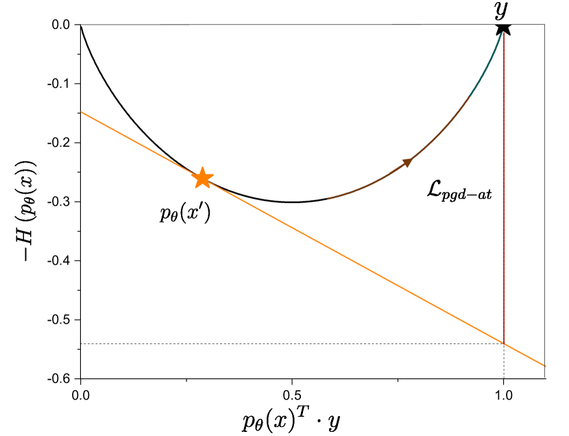
(a) PGD-AT

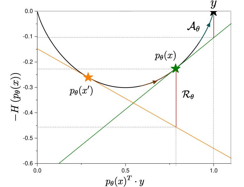
(b) TRADES

Figure 2: Illustrations of the Bregman divergence perspective of PGD-AT and TRADES.

3.2.1 Guideline 1: It is better to separate than to merge.

Lemma 1.

Given points $x_{1}$, $x_{2}$ and $x_{*}$, if $\exists\alpha\in[0,1]$ such that $p_{\theta}(x_{*})=(1-\alpha)p_{\theta}(x_{1})+\alpha p_{\theta}(x_{2})$, then the following inequality holds true:

$$KL(p_{\theta}(x_{2})\|p_{\theta}(x_{1}))\geq KL(p_{\theta}(x_{2})\|p_{\theta}(x_{*}))$$

$$+KL(p_{\theta}(x_{*})\|p_{\theta}(x_{1})).$$

We leave the proof of Lemma 1 to the supplementary materials. In the binary classification case, we actually have $p_{\theta}(x)=\alpha y+(1-\alpha)p_{\theta}(x^{\prime}),\alpha\in[0,1]$, because $x^{\prime}$ is harder to classify than $x$. According lemma 1, we can thus deduce that when $\lambda=1$ in Eq. (3), the loss term $\mathcal{L}_{trades}$ is lower than $\mathcal{L}_{pgd-at}$:

$$\mathcal{L}_{pgd-at}\geq\mathcal{L}_{trades}=\mathcal{A}_{\theta}+\mathcal{R}_{\theta},$$ (9)

as intuitively shown in Fig. 2(a) and Fig. 2(b). Eq. (9) indicates that the separation of the learning objective does not only makes TRADES able to balance the robustness-accuracy tradeoff but also reduces its optimization difficulty compared to that of PGD-AT. As a result, TRADES can adopt a larger $\lambda>1$ and attain better robustness than PGD-AT when $\lambda$ increases to the best robustness-accuracy tradeoff value. Nevertheless, the optimization of the robustness loss $\mathcal{R}_{\theta}$ remains difficult. Therefore, we think:

As TRADES is the separation of PGD-AT which reduces the optimization difficulty, can we separate the $\mathcal{R}_{\theta}$ again to make TRADES easier to train?

Motivated by this idea, we proposed the FAIT, which separates $\mathcal{R}_{\theta}$ into two smaller units by introducing an interpolated PGD adversary. We will introduce this method in more detail in Sec. 4, but before we do, let us introduce our other interesting finding.

3.2.2 Guideline 2: High-entropy models are better robustness learners.

As discussed, from the Bregman divergence perspective of AT, the training data slide on the negative entropy curve. This motivates us to study the function of entropy in AT. Specifically, we aim to answer the following question:

In AT, is a model with higher entropy better,
or is a model with lower entropy better?

To study this question, comparing the entropy values of different models is necessary, and we first give the following definition:

Definition 3.1 (Entropy upper bound).

Given two models $f_{\theta_{1}}$ and $f_{\theta_{2}}$, $\forall\tilde{x}\in\mathcal{B}(\mathcal{D},\epsilon)$, if the entropy of $\tilde{x}$ satisfies $H(p_{\theta_{1}}(\tilde{x}))\leq H(p_{\theta_{2}}(\tilde{x}))$, then we call model $f_{\theta_{2}}$ the entropy upper bound of model $f_{\theta_{1}}$ at a radius of $\epsilon$; this is denoted as $\mathcal{H}(f_{\theta_{1}},\epsilon)\leq\mathcal{H}(f_{\theta_{2}},\epsilon).$

When we have two models $f_{\theta_{1}}$ and $f_{\theta_{2}}$, however, it is not sufficient to analyze their optimization difficulty levels when $f_{\theta_{1}}$ and $f_{\theta_{2}}$ only satisfy $\mathcal{H}(f_{\theta_{1}},\epsilon)\leq\mathcal{H}(f_{\theta_{2}},\epsilon)$. For example, given an initial model with large entropy and a well-trained model with small entropy, it is inappropriate to compare the optimization difficulty levels of these two models because training the initial model is obviously much easier. That is, the convergence degrees of the two models should be similar for a fair comparison. Therefore, we give the following definition to ensure that the two models have the similar convergence degrees in the adversarial context.

Definition 3.2 (Identical adv-convergence).

$\forall\tilde{x}\in\mathcal{B}(\mathcal{D},\epsilon)$, if model $f_{\theta_{1}}$ and $f_{\theta_{2}}$ satisfy:

$$\mathop{\arg\max}_{i}p_{\theta_{1}}(\tilde{x})_{i}=\mathop{\arg\max}_{i}p_{\theta_{2}}(\tilde{x})_{i}$$

then $f_{\theta_{1}}$ has identical adv-convergence with $f_{\theta_{2}}$, and this is denoted as $\mathbb{I}(f_{\theta_{1}},\epsilon)=\mathbb{I}(f_{\theta_{2}},\epsilon).$

When $\mathbb{I}(f_{\theta_{1}},\epsilon)=\mathbb{I}(f_{\theta_{2}},\epsilon),$ it is easy to infer that $f_{\theta_{1}}$ and $f_{\theta_{2}}$ have the same the accuracy and robustness. That is, $f_{\theta_{1}}$ and $f_{\theta_{2}}$ will maintain the same robustness-accuracy tradeoff without the need to maintain the same entropy, and this property is useful for the analysis process.

In the binary classification case, there are three conditions regarding the clean output distribution $p_{\theta_{1}}(x)$ and the adversarial output distribution $p_{\theta_{1}}(x^{\prime})$ in model $f_{\theta_{1}}$: $\mathcal{C}.1$: $p_{\theta_{1}}(x)^{T}\cdot y>\frac{1}{2},p_{\theta_{1}}(x^{\prime})^{T}\cdot y\leq\frac{1}{2}$; $\mathcal{C}.2$: $p_{\theta_{1}}(x)^{T}\cdot y\leq\frac{1}{2},p_{\theta_{1}}(x^{\prime})^{T}\cdot y\leq\frac{1}{2}$; $\mathcal{C}.3$: $p_{\theta_{1}}(x)^{T}\cdot y>\frac{1}{2},p_{\theta_{1}}(x^{\prime})^{T}\cdot y>\frac{1}{2}$. Given a model $f_{\theta_{2}}$ that satisfies $\mathcal{H}(f_{\theta_{1}},\epsilon)\leq\mathcal{H}(f_{\theta_{2}},\epsilon)$ and $\mathbb{I}(f_{\theta_{1}},\epsilon)=\mathbb{I}(f_{\theta_{2}},\epsilon)$, we have the following two theorems for these different conditions.

Theorem 1 ($\mathcal{C}.1$).

Given $\mathcal{H}(f_{\theta_{1}},\epsilon)\leq\mathcal{H}(f_{\theta_{2}},\epsilon)$ and $\mathbb{I}(f_{\theta_{1}},\epsilon)=\mathbb{I}(f_{\theta_{2}},\epsilon)$, $\forall x\in\mathcal{D}$, if $\mathcal{C}.1$ holds true, then we have $\mathcal{R}_{\theta_{1}}(x,x^{\prime})\geq\mathcal{R}_{\theta_{2}}(x,x^{\prime})$.

Theorem 2 ($\mathcal{C}.2,\mathcal{C}.3$).

Define the difference between the clean and the adversarial probability distribution as $d_{\theta}(x,x^{\prime})=p_{\theta}(x)-p_{\theta}(x^{\prime})$ . Given $\mathcal{H}(f_{\theta_{1}},\epsilon)\leq\mathcal{H}(f_{\theta_{2}},\epsilon)$ and $\mathbb{I}(f_{\theta_{1}},\epsilon)=\mathbb{I}(f_{\theta_{2}},\epsilon)$, $\forall x\in\mathcal{D}$, if $\mathcal{C}.2$ or $\mathcal{C}.3$ holds true, let $d_{\theta_{1}}(x,x^{\prime})=d_{\theta_{2}}(x,x^{\prime})$, we also have $\mathcal{R}_{\theta_{1}}(x,x^{\prime})\geq\mathcal{R}_{\theta_{2}}(x,x^{\prime})$.

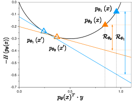
(a) $\mathcal{C}.1$

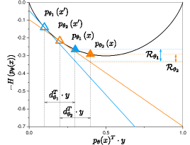
(b) $\mathcal{C}.2$

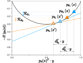
(c) $\mathcal{C}.3$

Figure 3: Illustrations of $R_{\theta}$ in models $f_{\theta_{1}}$ and $f_{\theta_{2}}$ when $\mathcal{H}(f_{\theta_{1}},\epsilon)\leq\mathcal{H}(f_{\theta_{2}},\epsilon)$ at the three different conditions.

3.2.3 Remark 1.

Proofs are provided in the supplementary materials. Theorem 3 and Theorem 4 tell us the following.

When two models keep the same robustness-accuracy tradeoff, the robustness loss $\mathcal{R}_{\theta}$ of the model with higher entropy is easier to optimize.

We provide the corresponding illustrations of the three conditions in Fig. 3 for better understanding. Based on this analysis, we introduce the MER strategy to maximize the entropy of the robust model, and we find that MER can effectively reduce the difficulty of optimizing $\mathcal{R}_{\theta}$.

4 Method

Based on the above analyses, in this section, we introduce two methods for mitigating the optimization difficulty of $\mathcal{R}_{\theta}$. The first is FAIT, which incorporate an interpolated PGD adversary into the training process. The second is MER, which maximizes the entropy of the output distribution.

4.1 FAIT

To further reduce the training difficulty of TRADES, we propose FAIT. FAIT separates $\mathcal{R}_{\theta}$ in TRADES by adding a new interpolation data point $x^{*}$, and replacing $\mathcal{R}_{\theta}$ with $\mathcal{R}^{\prime}_{\theta}$:

$$\mathcal{R}^{\prime}_{\theta}(x,x^{*},x^{\prime})=KL(p_{\theta}(x)\|p_{\theta}(x^{*}))+KL(p_{\theta}(x^{*})\|p_{\theta}(x^{\prime})).$$

There are various choices of $x^{*}$ only if that $x^{*}$ is more adversarial than $x$ and less adversarial than $x^{\prime}$. To avoid introducing extra computational overhead for generating $x^{*}$, we sample $x^{*}$ from the PGD iteration process with a fixed interpolation number $I(0<I<K)$, where $K$ is the number of PGD iterations. In the inner maximization, we keep using the KL-divergence as the loss function to retain the same 10-step PGD adversary of TRADES. In Algorithm 1, the pseudocode of FAIT is displayed for a more detailed understanding.

Algorithm 1 Friendly Adversarial Interpolation Training

Input: Training dataset $D^{N}_{train}$

Parameter: Batch size $m$; learning rate $\eta_{lr}$; PGD step size $\eta_{pgd}$; number of PGD iterations $K$; perturbation size $\epsilon$; PGD interpolation number $I$;

1:Randomly initialize the network parameters $\theta$

2:Set $\mathcal{L}_{fait}(x,x^{*},x^{\prime},y;\theta)=CE(p_{\theta}(x),y)+\lambda\cdot\mathcal{R}^{\prime}_{\theta}(x,x^{*},x^{\prime})$

3:repeat

4:     Sample a mini-batch $\{(x_{i},y_{i})\}_{i=1}^{m}$ from $D_{train}^{N}$

5:     for $i=1,2,...,m$ do

6:         $x_{i}^{\prime}\leftarrow x_{i}+0.001\cdot\mathcal{N}(0,I)$

7:         for $k=1,2,...K$ do

8:              $x^{\prime}_{i}\leftarrow\Pi_{\mathcal{B}(x_{i},\epsilon)}(x_{i}^{\prime}+\eta_{pgd}\cdot sign(\nabla_{x_{i}^{\prime}}KL(p_{\theta}(x_{i}),p_{\theta}(x_{i}^{\prime})))$ $\triangleright$ Generate $x^{\prime}$

9:              if $k=I$ then

10:                  $x_{i}^{*}\leftarrow x_{i}^{\prime}$ $\triangleright$ Sample $x^{*}$

11:              end if

12:         end for

13:     end for

14:     $g_{fait}=\frac{1}{m}\sum_{i=1}^{m}\nabla_{\theta}\mathcal{L}_{fait}(x_{i},x_{i}^{*},x_{i}^{\prime},y;\theta)$

15:     $\theta\leftarrow\theta-\eta_{lr}\cdot g_{fait}$

16:until training completed

Connection with FAT. Both FAIT and FAT [42] introduced weaker PGD adversaries into AT, with the aim of reducing the difficulty of optimization. However, FAT discards the 10-step PGD adversary. Because generalizing to the unseen data is much harder, FAT is limited in its ability to achieve better robustness. Different from FAT, FAIT still employs the 10-step PGD adversary, as we shall see in Table 1, FAIT can thus provide better robustness than FAT.

4.2 MER

The MER strategy has been widely studied in many areas of machine learning [11, 17, 26, 23]. Nevertheless, to the best of our knowledge, the effectiveness of MER in AT has not been investigated. The idea of MER is quite simple; by adding a negative entropy term in the original learning objective, the objective of MER is defined as:

$$\mathop{\arg\min}_{\theta}\mathbb{E}\{\mathcal{L}(x,y;\theta)-\beta\cdot H(p_{\theta}(x))\}.$$

However, in AT, the implementation of MER can be slightly more complicated. In addition to maximizing the entropy of the clean output distribution $p_{\theta}(x)$, maximizing the entropy of the adversarial output distribution $p_{\theta}(x^{\prime})$ is also optional. Therefore, when adding the MER into TRADES, we have the following objective:

$$\mathop{\arg\min}_{\theta}\mathbb{E}\{CE(p_{\theta}(x),y)+\lambda\cdot KL(p_{\theta}(x)\|p_{\theta}(x^{\prime}))$$ (10)

$$-(\beta_{cle}\cdot H(p_{\theta}(x))+\beta_{adv}\cdot H(p_{\theta}(x^{\prime})))\}.$$

We refer to this new learning objective as the TRADES-MER.

MER is compatible with FAIT. According to Lemma 1, $\mathcal{R}_{\theta}$ is an upper bound of $\mathcal{R}^{\prime}_{\theta}$. As discussed, $\mathcal{R}_{\theta}$ is easier to optimize in a model with higher entropy; therefore, MER can help reduce the upper bound of the $\mathcal{R}^{\prime}_{\theta}$, which makes $\mathcal{R}^{\prime}_{\theta}$ easier to optimize. Thus, MER should be compatible with FAIT. Experimental results have demonstrated this point of view. As we shall see in Table 4, FAIT-MER has better robustness than both FAIT and TRADES-MER.

5 Experiments

Training settings. In the basic settings, we apply ResNet-18 [13] as the model architecture, but we also provide results of other architectures in Table 5. To generate the PGD adversaries, we set the step size $\eta_{pgd}=2/255$ and the perturbation size $\epsilon=8/255$ under the $\ell_{\infty}$ norm, and the number of iterations is set to $K=10$. During the training process, we use the SGD optimizer with a weight decay of $5\times 10^{-4}$ and momentum 0.9. We use a large batch size $m=512$ to speed up the training. We train models for 100 epochs, and the initial learning rate is 0.4 and decays by a factor of 0.1 at epochs 75 and 90. In addition, we introduce an extra 5 epochs to gradually warm up [12] the model at the beginning to alleviate the performance degeneration caused by the large batch size.

Robustness estimation. We evaluate the robustness of the model by using PGD attacks and AA [8]. Among them, the PGD attacks is less computationally expensive; thus, we evaluate the PGD robustness after per epoch training and record the epoch with the best robustness for further estimation. AA is a more advanced attack to verify the robustness via an ensemble of four diverse parameter-free attacks including three white-box attacks: APGD-CE [8], APGD-DLR [8], FAB [9] and a black-box attack: Square Attack [3], which has been consistently shown to provide reliable robustness estimates.

Reproducibility. We report the results average over 3 runs obtained on a machine with 4 RTX 2080 Ti GPUs, and the code is provided in the supplementary materials and will be made public after the review process is completed.

5.1 Do FAIT and MER reduce the difficulty of optimization?

We first provide the obtained experimental results to support our proposition that FAIT and MER can reduce the difficulty of optimizing $\mathcal{R}_{\theta}$. In Fig. 4, we plot the curves of $\mathcal{R}_{\theta}$ and $\mathcal{R}_{\theta}^{\prime}$ for each training epoch of TRADES ($\lambda=9$) and TRADES-MER ($\lambda=9$).

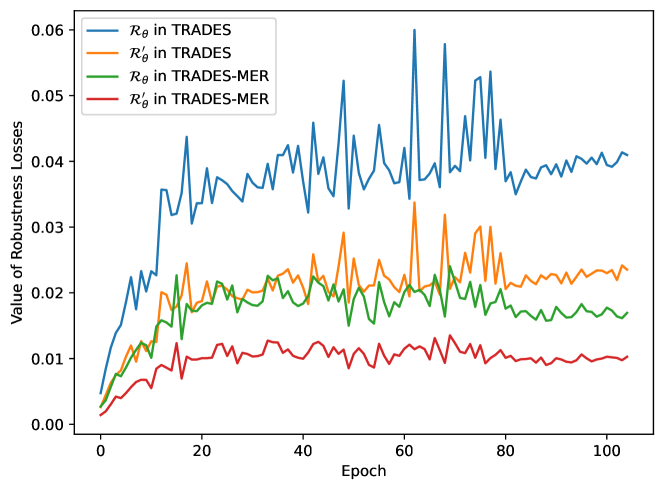
Figure 4: Results of $\mathcal{R}_{\theta}$ and $\mathcal{R}_{\theta}^{\prime}$ during the training process of TRADES and TRADES-MER with the same $\lambda=9$.

We obtained both $\mathcal{R}_{\theta}$ and $\mathcal{R}_{\theta}^{\prime}$ by averaging the values obtained over a thousand examples in the CIFAR-10 training set [18], and $\mathcal{R}_{\theta}^{\prime}$ is calculated with $I=2$. We can see that

1. $\mathcal{R}_{\theta}^{\prime}$ is lower than $\mathcal{R}_{\theta}$ during the training process of both TRADES and TRADES-MER. As $\mathcal{R}_{\theta}^{\prime}$ and $\mathcal{R}_{\theta}$ denote the robustness loss term of FAIT and TRADES, respectively, this empirical result indicates that the FAIT robustness loss is lower than that the TRADES robustness loss, which is consistent with the Lemma 1.

2. $\mathcal{R}_{\theta}$ in TRADES-MER is lower than $\mathcal{R}_{\theta}$ in TRADES while both TRADES-MER and TRADES train with the same $\lambda=9$ and this empirical result is consistent with our Theorem 3 and Theorem 4.

These results demonstrate that FAIT and MER can indeed help reduce the optimization difficulty of $\mathcal{R}_{\theta}$ in TRADES.

5.2 Do FAIT and MER enhance the adversarial robustness?

5.2.1 Larger $\lambda$ values and better robustness.

Because FAIT and MER can help reduce the difficulty of optimizing the $\mathcal{R}_{\theta}$, we find that both TRADES-MER and FAIT can thus adopt larger $\lambda$ values than TRADES, and more importantly, when $\lambda$ increases to the optimal robustness-accuracy tradeoff value, our methods also attain better robustness. In Table 1, we report the accuracy and AA robustness of TRADES, as well as the FAT for TRADES [42], FAIT and TRADES-MER with different $\lambda$ values on the CIFAR-10 test set with ResNet-18. For FAIT, we use $I=2$, and for TRADES-MER we use {$\beta_{cle}=1,\beta_{adv}=0$}, and we provide the parametric search results of $I$ and {$\beta_{cle},\beta_{adv}$} in Table 2 and Table 3, respectively.

We bold the best AA result of each method. As shown in Table 1, when TRADES, FAIT and TRADES-MER reach the best robustness at $\lambda=9$, $\lambda=12$ and $\lambda=21$, the robustness of FAIT and TRADES-MER are both stronger than TRADES. In addition, we can see that FAIT gains better robustness than FAT for TRADES, which demonstrates that using the 10-step PGD adversary is important for guaranteeing robustness.

$\lambda$	TRADES		FAT for TRADES		FAIT (ours)		TRADES-MER (ours)
	Clean	AA	Clean	AA	Clean	AA	Clean	AA
3	83.62$\pm$0.25	46.92$\pm$0.15	84.45$\pm$0.36	45.75$\pm$0.14	84.98$\pm$0.81	46.84$\pm$1.11	87.14$\pm$0.17	44.22$\pm$0.13
6	81.45$\pm$0.19	48.04$\pm$0.16	82.48$\pm$0.34	47.48$\pm$0.23	83.20$\pm$0.17	48.82$\pm$0.11	85.64$\pm$0.17	46.58$\pm$0.25
9	79.42$\pm$0.05	48.53$\pm$0.19	81.06$\pm$0.27	47.98$\pm$0.11	81.37$\pm$0.06	49.40$\pm$0.34	84.69$\pm$0.07	47.82$\pm$0.05
12	77.91$\pm$0.18	48.20$\pm$0.33	80.27$\pm$0.32	48.08$\pm$0.32	80.31$\pm$0.16	49.41$\pm$0.1	83.52$\pm$0.39	48.71$\pm$0.5
15	76.60$\pm$0.15	48.39$\pm$0.18	79.41$\pm$0.06	48.48$\pm$0.13	79.03$\pm$0.09	49.15$\pm$0.13	82.54$\pm$0.05	48.39$\pm$0.32
18	75.74$\pm$0.39	47.72$\pm$0.4	78.78$\pm$0.35	48.16$\pm$0.15	78.36$\pm$0.09	49.05$\pm$0.04	81.58$\pm$0.07	48.69$\pm$0.33
21	75.03$\pm$0.46	47.64$\pm$0.26	78.18$\pm$0.3	48.40$\pm$0.19	77.18$\pm$0.3	48.72$\pm$0.16	81.23$\pm$0.18	49.04$\pm$0.25

Table 1: CIFAR-10 results of TRADES, FAT for TRADES, FAIT and TRADES-MER with various $\lambda$.

$I$	1	2	3	4	5	6	7	8	9
Clean	79.29	80.31	80.57	78.99	78.32	78.80	78.03	77.73	78.30
AA	49.07	49.41	48.89	48.70	49.02	49.13	49.27	48.46	48.75

Table 2: The parameter $I$ in FAIT with $\lambda=12$.

$\beta_{cle}$	$\beta_{adv}$	Clean	AA
0	1	81.14	48.9
0.5	0.5	81.37	48.69
1	0	81.23	49.04

Table 3: The parameters $\beta_{cle}$ and $\beta_{adv}$ in TRADES-MER with $\lambda=21$.

Method	CIFAR-10			CIFAR-100
	Clean	PGD-100	AA	Clean	PGD-100	AA
PGD-AT	83.59$\pm$0.24	48.68$\pm$0.15	45.83$\pm$0.1	58.97$\pm$0.1	25.58$\pm$0.39	22.79$\pm$0.31
GAIRAT	83.21$\pm$0.23	49.30$\pm$0.33	46.82$\pm$0.28	56.73$\pm$0.25	24.78$\pm$0.17	22.00$\pm$0.15
MART	78.49$\pm$0.51	52.71$\pm$0.18	46.24$\pm$0.17	53.3$\pm$0.16	30.08$\pm$0.26	24.61$\pm$0.24
TRADES-AWP	81.23$\pm$0.21	51.77$\pm$0.06	48.62$\pm$0.03	57.02$\pm$0.13	28.97$\pm$0.33	24.56$\pm$0.12
HAT	84.98$\pm$0.14	51.61$\pm$0.14	48.63$\pm$0.22	60.18$\pm$0.33	26.84$\pm$0.46	22.62$\pm$0.34
FAIT ($\lambda=12$)	80.31$\pm$0.16	53.04$\pm$0.08	49.41$\pm$0.1	57.14$\pm$0.19	29.38$\pm$0.03	24.79$\pm$0.07
TRADES-MER ($\lambda=21$)	81.23$\pm$0.18	53.4$\pm$0.27	49.04$\pm$0.25	58.64$\pm$0.08	30.04$\pm$0.12	24.63$\pm$0.26
FAIT-MER ($\lambda=30$)	81.4$\pm$0.28	53.87$\pm$0.24	49.49$\pm$0.37	58.87$\pm$0.11	30.48$\pm$0.06	24.84$\pm$0.12

Table 4: Comparison of the state of the art AT methods with ResNet-18.

5.2.2 Compare with more AT methods.

To further check the effectiveness of the proposed FAIT and MER methods, we compare them with a batch of the state of art AT methods: PGD-AT [21], GAIRAT [43], MART [35], TRADES-AWP [37] and HAT [27]. We reproduce the learning objectives of PGD-AT, MART and TRADES-AWP in our code, and for GAIRAT and HAT, we use the original code found in their GitHub repositories.

In Table 4, we report the results obtained on the CIFAR-10 and CIFAR-100 datasets with ResNet-18, and we can see that FAIT and TRADES-MER again outperform the previous works in terms of robustness. In particular, when we combine FAIT with MER (the FAIT-MER), we found that the ResNet-18 model can adopt an enormous $\lambda$ with a value of 30, and FAIT-MER outperforms FAIT and TRADES-MER in robustness to both PGD-100 attacks and AA, which demonstrates the compatibility of FAIT and MER.

5.3 Scalability

5.3.1 Different model architectures.

In Table 5, we show the CIFAR-10 results obtained by TRADES, FAIT and TRADES-MER under three different model architectures: SENET18 [14], VGG16 [31] and ShuffleNetv2 [20]. We continue to use the best group of hyperparameters in our ResNet-18 experiments, where $\{\lambda=12,I=2\}$ for FAIT and $\{\lambda=21,\beta_{cle}=1,\beta_{adv}=0\}$ for TRADES-MER. Even though we do not search for the best robustness-accuracy tradeoff hyperparameters for these three architectures, we find that FAIT and TRADES-MER can still outperform TRADES, which demonstrates the scalability of our methods to different model architectures.

5.3.2 Different $\psi$ functions also work well.

Recall that the Bregman divergence is parameterized by the convex function $\psi$, as described in Eq. (6); however, our previous analyses of PGD-AT and TRADES were based on $\psi=-H$, which leaves the following question: can FAIT and MER still work when $\psi$ changes to another function?

Furthermore, we notice that a recent work [25] theoretically showed that the KL-divergence in TRADES can be substituted for various statistical distances. Among them, the square error (SE) has been shown to be the most effective one, outperforming the KL-divergence, and this idea is called as the Self-COnsistent Robust Error (SCORE). Because the SE is also a Bregman divergence whose $\psi$ is the squaring function,

$$\psi(p)=S(p)=\sum p_{i}^{2}.$$

Therefore, we plan to check the effectiveness of FAIT and MER under $\psi=S$. To do so, we first follow the implementation of SCORE by replacing the KL-divergence in both the inner maximization and outer minimization operations of TRADES with the SE. Then, we expand FAIT and MER to the SE versions. For FAIT, there is no other difference from Algorithm 1. For MER, we maximize $-S$ rather than maximizing the entropy function $H$. We denote the FAIT and MER methods under $\psi=S$ as FAIT_ψ=S and TRADES-MER_ψ=S, respectively.

Method	SENET18		VGG16		ShuffleNetv2
	Clean	AA	Clean	AA	Clean	AA
TRADES	81.63	49.41	77.48	43.46	71.84	38.32
FAIT	81.70	49.60	78.21	44.63	72.35	38.45
TRADES-MER	81.94	49.71	76.97	43.60	71.79	38.67

Table 5: Performance under various model architectures.

Method	$\lambda$		CIFAR-10
			Clean	PGD-100	AA
SCORE	4		83.94	52.94	49.04
FAITψ=S	8		82.11	53.93	49.48
TRADES-MERψ=S	10		82.56	54.21	49.42

Table 6: FAIT and TRADES-MER with $\psi=S$.

In Table 6, we report the CIFAR-10 results of SCORE, FAIT_ψ=S and TRADES-MER_ψ=S with ResNet-18. For SCORE, we use $\lambda=4$ according to Pang et al., and we can see that both FAIT_ψ=S and TRADES-MER_ψ=S can adopt larger $\lambda$ values at the value of 8 and 10, respectively. Besides, both of them again achieve better robustness, which demonstrates the scalability of our methods when $\psi$ changes.

6 Conclusion

In this paper, we demonstrated that reducing the difficulty of optimizing the robustness loss $\mathcal{R}_{\theta}$ under 10-step PGD adversaries is a promising approach for enhancing adversarial robustness. We build a novel Bregman divergence perspective for AT to clearly look at the optimization problem concerning $\mathcal{R}_{\theta}$. Based on this perspective, we propose FAIT and MER and verify that both of them can help enhance adversarial robustness and are easier to optimize than their prototype method TRADES. We hope that this novel perspective and our analyses will help future works design more robust DNN models and AT algorithms.

7 Acknowledgments

This work was sponsored by Zhejiang Laboratory(No. 2021KD0AB03).

Appendix A Proofs

Lemma 2.

Given points $x_{1}$, $x_{2}$ and $x_{*}$, if $\exists\alpha\in[0,1]$ such that $p_{\theta}(x_{*})=(1-\alpha)p_{\theta}(x_{1})+\alpha p_{\theta}(x_{2})$, then the following inequality holds true:

$$KL(p_{\theta}(x_{2})\|p_{\theta}(x_{1}))\geq KL(p_{\theta}(x_{2})\|p_{\theta}(x_{*}))$$

$$+KL(p_{\theta}(x_{*})\|p_{\theta}(x_{1})).$$

Proof of Lemma 2.

According to the laws of cosines, we have:

$$KL(p_{\theta}(x_{2})\|p_{\theta}(x_{1}))$$ (11)

$$-KL(p_{\theta}(x_{2})\|p_{\theta}(x_{*}))-KL(p_{\theta}(x_{*})\|p_{\theta}(x_{1}))$$

$$= -\sum(p_{\theta}(x_{2})_{i}-p_{\theta}(x_{*})_{i})(\nabla-H(p_{\theta}(x_{1}))_{i}$$

$$-\nabla-H(p_{\theta}(x_{*}))_{i})$$

$$= \sum(1-\alpha)\cdot$$

$$\underbrace{(p_{\theta}(x_{2})_{i}-p_{\theta}(x_{1})_{i})}_{\lower 2.1097pt\hbox{ \leavevmode\hbox to11.67pt{\vbox to10.47pt{\text{[drawing]}}}}}\underbrace{(log(1-\alpha+\alpha\frac{p_{\theta}(x_{2})_{i}}{p_{\theta}(x_{1})_{i}}))}_{\lower 2.1097pt\hbox{ \leavevmode\hbox to11.67pt{\vbox to10.47pt{\text{[drawing]}}}}}.$$

Since $\alpha\in[0,1]$, we have $1-\alpha\geq 0$. $\forall x_{1},x_{2}$, if $p_{\theta}(x_{2})_{i}>p_{\theta}(x_{1})_{i}$, we have $\lower 3.01385pt\hbox{ \leavevmode\hbox to16.67pt{\vbox to12.47pt{\text{[drawing]}}}}>0$ and $\lower 3.01385pt\hbox{ \leavevmode\hbox to16.67pt{\vbox to12.47pt{\text{[drawing]}}}}>0$, respectively. If $p_{\theta}(x_{2})_{i}\leq p_{\theta}(x_{1})_{i}$, we have $\lower 3.01385pt\hbox{ \leavevmode\hbox to16.67pt{\vbox to12.47pt{\text{[drawing]}}}}\leq 0$ and $\lower 3.01385pt\hbox{ \leavevmode\hbox to16.67pt{\vbox to12.47pt{\text{[drawing]}}}}\leq 0$, too. Therefore, Eq. (11)$\geq 0$, and Lemma 1 holds true. ∎

Theorem 3 ($\mathcal{C}.1$).

Given $\mathcal{H}(f_{\theta_{1}},\epsilon)\leq\mathcal{H}(f_{\theta_{2}},\epsilon)$ and $\mathbb{I}(f_{\theta_{1}},\epsilon)=\mathbb{I}(f_{\theta_{2}},\epsilon)$, $\forall x\in\mathcal{D}$, if $\mathcal{C}.1$ holds true, then we have $\mathcal{R}_{\theta_{1}}(x,x^{\prime})\geq\mathcal{R}_{\theta_{2}}(x,x^{\prime})$.

Theorem 4 ($\mathcal{C}.2,\mathcal{C}.3$).

Define the difference between the clean and the adversarial probability distribution as $d_{\theta}(x,x^{\prime})=p_{\theta}(x)-p_{\theta}(x^{\prime})$ . Given $\mathcal{H}(f_{\theta_{1}},\epsilon)\leq\mathcal{H}(f_{\theta_{2}},\epsilon)$ and $\mathbb{I}(f_{\theta_{1}},\epsilon)=\mathbb{I}(f_{\theta_{2}},\epsilon)$, $\forall x\in\mathcal{D}$, if $\mathcal{C}.2$ or $\mathcal{C}.3$ holds true, let $d_{\theta_{1}}(x,x^{\prime})=d_{\theta_{2}}(x,x^{\prime})$, we also have $\mathcal{R}_{\theta_{1}}(x,x^{\prime})\geq\mathcal{R}_{\theta_{2}}(x,x^{\prime})$.

Proof of Theorem 3.

For $\mathcal{C}.1$ holds true, model $f_{\theta_{1}}$ and $f_{\theta_{2}}$ satisfy that $\mathcal{H}(f_{\theta_{1}},\epsilon)\leq\mathcal{H}(f_{\theta_{2}},\epsilon)$ and $\mathbb{I}(f_{\theta_{1}},\epsilon)=\mathbb{I}(f_{\theta_{2}},\epsilon)$, we have:

$$p_{\theta_{1}}(x)^{T}\cdot y\geq p_{\theta_{2}}(x)^{T}\cdot y>p_{\theta_{2}}(x^{\prime})^{T}\cdot y\geq p_{\theta_{1}}(x^{\prime})^{T}\cdot y$$

Therefore, in the binary classification case, $\exists\alpha_{1},\alpha_{2}\in[0,1]$ such that

$$p_{\theta_{2}}(x)=(1-\alpha_{1})p_{\theta_{1}}(x^{\prime})+\alpha_{1}p_{\theta_{1}}(x)$$

$$p_{\theta_{2}}(x^{\prime})=(1-\alpha_{2})p_{\theta_{1}}(x^{\prime})+\alpha_{2}p_{\theta_{2}}(x)$$

According to Lemma 2, we have:

$$R_{\theta_{1}}(x,x^{\prime})$$ (12)

$$= KL(p_{\theta_{1}}(x)\|p_{\theta_{1}}(x^{\prime}))$$

$$\geq KL(p_{\theta_{1}}(x)\|p_{\theta_{2}}(x))+KL(p_{\theta_{2}}(x)\|p_{\theta_{1}}(x^{\prime}))$$

$$\geq KL(p_{\theta_{1}}(x)\|p_{\theta_{2}}(x))$$

$$+KL(p_{\theta_{2}}(x)\|p_{\theta_{2}}(x^{\prime}))+KL(p_{\theta_{2}}(x^{\prime})\|p_{\theta_{1}}(x^{\prime}))$$

$$= KL(p_{\theta_{1}}(x)\|p_{\theta_{2}}(x))$$

$$+KL(p_{\theta_{2}}(x^{\prime})\|p_{\theta_{1}}(x^{\prime}))+R_{\theta_{2}}(x,x^{\prime})$$

Because KL-divergence is not negative, we have $R_{\theta_{1}}(x,x^{\prime})\geq R_{\theta_{2}}(x,x^{\prime})$, thus Theorem 3 holds true. ∎

Proof of Theorem 4.

Let $\Delta=d_{\theta}(x,x^{\prime})^{T}\cdot y$, and because $x^{\prime}$ is more likely to be misclassified than $x$, we have $\Delta>0$. Let $t=p_{\theta}(x^{\prime})^{T}\cdot y$, we have:

$$KL(p_{\theta}(x)\|p_{\theta}(x^{\prime}))$$

$$= (t+\Delta)log(\frac{t+\Delta}{t})+(1-t-\Delta)log(\frac{1-t-\Delta}{1-t}).$$

Let $F(t)=-log(\frac{1-t}{t})$, then

$$\frac{\mathrm{d}}{\mathrm{d}t}KL(p_{\theta}(x)\|p_{\theta}(x^{\prime}))$$ (13)

$$= log(\frac{t+\Delta}{t})-\frac{\Delta}{t}-log(\frac{1-t-\Delta}{1-t})-\frac{\Delta}{1-t}$$

$$= log(\frac{1-t}{t}\cdot\frac{t+\Delta}{1-(t+\Delta)})-\frac{\Delta}{t(1-t)}$$

$$= F(t+\Delta)-F(t)-\frac{\Delta}{t(1-t)}$$

$$= F^{\prime}(\xi)\Delta-\frac{\Delta}{t(1-t)}$$

$$= \frac{\Delta}{\xi(1-\xi)}-\frac{\Delta}{t(1-t)},$$

where $t<\xi<t+\Delta$ according to the Lagrange’s mean value theorem. For model $f_{\theta_{1}}$ and $f_{\theta_{2}}$ satisfy that $\mathcal{H}(f_{\theta_{1}},\epsilon)\leq\mathcal{H}(f_{\theta_{2}},\epsilon)$ , $\mathbb{I}(f_{\theta_{1}},\epsilon)=\mathbb{I}(f_{\theta_{2}},\epsilon)$ and $d_{\theta_{1}}(x,x^{\prime})=d_{\theta_{2}}(x,x^{\prime}),\forall x\in\mathcal{D}$, we have

1. If $\mathcal{C}.2$ holds true, we have $0<p_{\theta_{1}}(x^{\prime})^{T}\cdot y\leq p_{\theta_{2}}(x^{\prime})^{T}\cdot y\leq\frac{1}{2}$, and for $0<t\leq\frac{1}{2}$, we have Eq. (13)$<0$, therefore we have $KL(p_{\theta_{1}}(x)\|p_{\theta_{1}}(x^{\prime}))\geq KL(p_{\theta_{2}}(x)\|p_{\theta_{2}}(x^{\prime}))$, i.e., $\mathcal{R}_{\theta_{1}}(x,x^{\prime})\geq\mathcal{R}_{\theta_{2}}(x,x^{\prime})$.

2. If $\mathcal{C}.3$ holds true, we have $\frac{1}{2}<p_{\theta_{2}}(x^{\prime})^{T}\cdot y\leq p_{\theta_{1}}(x^{\prime})^{T}\cdot y<1$, and for $\frac{1}{2}<t<1$, we have Eq. (13)$>0$, then we also have $\mathcal{R}_{\theta_{1}}(x,x^{\prime})\geq\mathcal{R}_{\theta_{2}}(x,x^{\prime})$. Therefore, Theorem 4 holds true. ∎

References

- Alayrac et al. [2019] Jean-Baptiste Alayrac, Jonathan Uesato, Po-Sen Huang, Alhussein Fawzi, Robert Stanforth, and Pushmeet Kohli. Are labels required for improving adversarial robustness? In Hanna M. Wallach, Hugo Larochelle, Alina Beygelzimer, Florence d’Alché-Buc, Emily B. Fox, and Roman Garnett, editors, Advances in Neural Information Processing Systems 32: Annual Conference on Neural Information Processing Systems 2019, NeurIPS 2019, December 8-14, 2019, Vancouver, BC, Canada, pages 12192–12202, 2019. URL https://proceedings.neurips.cc/paper/2019/hash/bea6cfd50b4f5e3c735a972cf0eb8450-Abstract.html.
- Andriushchenko and Flammarion [2020] Maksym Andriushchenko and Nicolas Flammarion. Understanding and improving fast adversarial training. In H. Larochelle, M. Ranzato, R. Hadsell, M.F. Balcan, and H. Lin, editors, Advances in Neural Information Processing Systems, volume 33, pages 16048–16059. Curran Associates, Inc., 2020. URL https://proceedings.neurips.cc/paper/2020/file/b8ce47761ed7b3b6f48b583350b7f9e4-Paper.pdf.
- Andriushchenko et al. [2020] Maksym Andriushchenko, Francesco Croce, Nicolas Flammarion, and Matthias Hein. Square attack: A query-efficient black-box adversarial attack via random search. In Andrea Vedaldi, Horst Bischof, Thomas Brox, and Jan-Michael Frahm, editors, Computer Vision - ECCV 2020 - 16th European Conference, Glasgow, UK, August 23-28, 2020, Proceedings, Part XXIII, volume 12368 of Lecture Notes in Computer Science, pages 484–501. Springer, 2020. doi: 10.1007/978-3-030-58592-1“˙29. URL https://doi.org/10.1007/978-3-030-58592-1_29.
- Bregman [1967] Lev M Bregman. The relaxation method of finding the common point of convex sets and its application to the solution of problems in convex programming. USSR computational mathematics and mathematical physics, 7(3):200–217, 1967.
- Carmon et al. [2019] Yair Carmon, Aditi Raghunathan, Ludwig Schmidt, John C. Duchi, and Percy Liang. Unlabeled data improves adversarial robustness. In Hanna M. Wallach, Hugo Larochelle, Alina Beygelzimer, Florence d’Alché-Buc, Emily B. Fox, and Roman Garnett, editors, Advances in Neural Information Processing Systems 32: Annual Conference on Neural Information Processing Systems 2019, NeurIPS 2019, December 8-14, 2019, Vancouver, BC, Canada, pages 11190–11201, 2019. URL https://proceedings.neurips.cc/paper/2019/hash/32e0bd1497aa43e02a42f47d9d6515ad-Abstract.html.
- Chen et al. [2021] Tianlong Chen, Zhenyu Zhang, Sijia Liu, Shiyu Chang, and Zhangyang Wang. Robust overfitting may be mitigated by properly learned smoothening. In 9th International Conference on Learning Representations, ICLR 2021, Virtual Event, Austria, May 3-7, 2021. OpenReview.net, 2021. URL https://openreview.net/forum?id=qZzy5urZw9.
- Cheng et al. [2022] Xu Cheng, Hao Zhang, Yue Xin, Wen Shen, Jie Ren, and Quanshi Zhang. Why adversarial training of relu networks is difficult? CoRR, abs/2205.15130, 2022. doi: 10.48550/arXiv.2205.15130. URL https://doi.org/10.48550/arXiv.2205.15130.
- Croce and Hein [2020a] Francesco Croce and Matthias Hein. Reliable evaluation of adversarial robustness with an ensemble of diverse parameter-free attacks. In Proceedings of the 37th International Conference on Machine Learning, ICML 2020, 13-18 July 2020, Virtual Event, volume 119 of Proceedings of Machine Learning Research, pages 2206–2216. PMLR, 2020a. URL http://proceedings.mlr.press/v119/croce20b.html.
- Croce and Hein [2020b] Francesco Croce and Matthias Hein. Minimally distorted adversarial examples with a fast adaptive boundary attack. In Proceedings of the 37th International Conference on Machine Learning, ICML 2020, 13-18 July 2020, Virtual Event, volume 119 of Proceedings of Machine Learning Research, pages 2196–2205. PMLR, 2020b. URL http://proceedings.mlr.press/v119/croce20a.html.
- Ding et al. [2020] Gavin Weiguang Ding, Yash Sharma, Kry Yik Chau Lui, and Ruitong Huang. MMA training: Direct input space margin maximization through adversarial training. In 8th International Conference on Learning Representations, ICLR 2020, Addis Ababa, Ethiopia, April 26-30, 2020. OpenReview.net, 2020. URL https://openreview.net/forum?id=HkeryxBtPB.
- Dubey et al. [2018] Abhimanyu Dubey, Otkrist Gupta, Ramesh Raskar, and Nikhil Naik. Maximum-entropy fine grained classification. In Samy Bengio, Hanna M. Wallach, Hugo Larochelle, Kristen Grauman, Nicolò Cesa-Bianchi, and Roman Garnett, editors, Advances in Neural Information Processing Systems 31: Annual Conference on Neural Information Processing Systems 2018, NeurIPS 2018, December 3-8, 2018, Montréal, Canada, pages 635–645, 2018. URL https://proceedings.neurips.cc/paper/2018/hash/0c74b7f78409a4022a2c4c5a5ca3ee19-Abstract.html.
- Goyal et al. [2017] Priya Goyal, Piotr Dollár, Ross B. Girshick, Pieter Noordhuis, Lukasz Wesolowski, Aapo Kyrola, Andrew Tulloch, Yangqing Jia, and Kaiming He. Accurate, large minibatch SGD: training imagenet in 1 hour. CoRR, abs/1706.02677, 2017. URL http://arxiv.org/abs/1706.02677.
- He et al. [2016] Kaiming He, Xiangyu Zhang, Shaoqing Ren, and Jian Sun. Deep residual learning for image recognition. In 2016 IEEE Conference on Computer Vision and Pattern Recognition, CVPR 2016, Las Vegas, NV, USA, June 27-30, 2016, pages 770–778. IEEE Computer Society, 2016. doi: 10.1109/CVPR.2016.90. URL https://doi.org/10.1109/CVPR.2016.90.
- Hu et al. [2017] Jie Hu, Li Shen, and Gang Sun. Squeeze-and-excitation networks. CoRR, abs/1709.01507, 2017. URL http://arxiv.org/abs/1709.01507.
- Ilyas et al. [2019] Andrew Ilyas, Shibani Santurkar, Dimitris Tsipras, Logan Engstrom, Brandon Tran, and Aleksander Madry. Adversarial examples are not bugs, they are features. Advances in neural information processing systems, 32, 2019.
- Jia et al. [2021] Xiaojun Jia, Yong Zhang, Baoyuan Wu, Jue Wang, and Xiaochun Cao. Boosting fast adversarial training with learnable adversarial initialization. CoRR, abs/2110.05007, 2021. URL https://arxiv.org/abs/2110.05007.
- Kim et al. [2019] Dahyun Kim, Jihwan Bae, Yeonsik Jo, and Jonghyun Choi. Incremental learning with maximum entropy regularization: Rethinking forgetting and intransigence. CoRR, abs/1902.00829, 2019. URL http://arxiv.org/abs/1902.00829.
- Krizhevsky et al. [2009] Alex Krizhevsky, Geoffrey Hinton, et al. Learning multiple layers of features from tiny images. 2009.
- Li et al. [2020] Bai Li, Shiqi Wang, Suman Jana, and Lawrence Carin. Towards understanding fast adversarial training. CoRR, abs/2006.03089, 2020. URL https://arxiv.org/abs/2006.03089.
- Ma et al. [2018] Ningning Ma, Xiangyu Zhang, Hai-Tao Zheng, and Jian Sun. Shufflenet V2: practical guidelines for efficient CNN architecture design. In Vittorio Ferrari, Martial Hebert, Cristian Sminchisescu, and Yair Weiss, editors, Computer Vision - ECCV 2018 - 15th European Conference, Munich, Germany, September 8-14, 2018, Proceedings, Part XIV, volume 11218 of Lecture Notes in Computer Science, pages 122–138. Springer, 2018. doi: 10.1007/978-3-030-01264-9“˙8. URL https://doi.org/10.1007/978-3-030-01264-9_8.
- Madry et al. [2018] Aleksander Madry, Aleksandar Makelov, Ludwig Schmidt, Dimitris Tsipras, and Adrian Vladu. Towards deep learning models resistant to adversarial attacks. In 6th International Conference on Learning Representations, ICLR 2018, Vancouver, BC, Canada, April 30 - May 3, 2018, Conference Track Proceedings. OpenReview.net, 2018. URL https://openreview.net/forum?id=rJzIBfZAb.
- Metzen et al. [2017] Jan Hendrik Metzen, Tim Genewein, Volker Fischer, and Bastian Bischoff. On detecting adversarial perturbations. arXiv preprint arXiv:1702.04267, 2017.
- Mnih et al. [2016] Volodymyr Mnih, Adrià Puigdomènech Badia, Mehdi Mirza, Alex Graves, Timothy P. Lillicrap, Tim Harley, David Silver, and Koray Kavukcuoglu. Asynchronous methods for deep reinforcement learning. In Maria-Florina Balcan and Kilian Q. Weinberger, editors, Proceedings of the 33nd International Conference on Machine Learning, ICML 2016, New York City, NY, USA, June 19-24, 2016, volume 48 of JMLR Workshop and Conference Proceedings, pages 1928–1937. JMLR.org, 2016. URL http://proceedings.mlr.press/v48/mniha16.html.
- Nakkiran [2019] Preetum Nakkiran. Adversarial robustness may be at odds with simplicity. CoRR, abs/1901.00532, 2019. URL http://arxiv.org/abs/1901.00532.
- Pang et al. [2022] Tianyu Pang, Min Lin, Xiao Yang, Jun Zhu, and Shuicheng Yan. Robustness and accuracy could be reconcilable by (proper) definition. arXiv preprint arXiv:2202.10103, 2022.
- Pereyra et al. [2017] Gabriel Pereyra, George Tucker, Jan Chorowski, Lukasz Kaiser, and Geoffrey E. Hinton. Regularizing neural networks by penalizing confident output distributions. In 5th International Conference on Learning Representations, ICLR 2017, Toulon, France, April 24-26, 2017, Workshop Track Proceedings. OpenReview.net, 2017. URL https://openreview.net/forum?id=HyhbYrGYe.
- Rade and Moosavi-Dezfooli [2021] Rahul Rade and Seyed-Mohsen Moosavi-Dezfooli. Reducing excessive margin to achieve a better accuracy vs. robustness trade-off. In International Conference on Learning Representations, 2021.
- Raghunathan et al. [2020] Aditi Raghunathan, Sang Michael Xie, Fanny Yang, John C. Duchi, and Percy Liang. Understanding and mitigating the tradeoff between robustness and accuracy. In Proceedings of the 37th International Conference on Machine Learning, ICML 2020, 13-18 July 2020, Virtual Event, volume 119 of Proceedings of Machine Learning Research, pages 7909–7919. PMLR, 2020. URL http://proceedings.mlr.press/v119/raghunathan20a.html.
- Schmidt et al. [2018] Ludwig Schmidt, Shibani Santurkar, Dimitris Tsipras, Kunal Talwar, and Aleksander Madry. Adversarially robust generalization requires more data. In Samy Bengio, Hanna M. Wallach, Hugo Larochelle, Kristen Grauman, Nicolò Cesa-Bianchi, and Roman Garnett, editors, Advances in Neural Information Processing Systems 31: Annual Conference on Neural Information Processing Systems 2018, NeurIPS 2018, December 3-8, 2018, Montréal, Canada, pages 5019–5031, 2018. URL https://proceedings.neurips.cc/paper/2018/hash/f708f064faaf32a43e4d3c784e6af9ea-Abstract.html.
- Shafahi et al. [2020] Ali Shafahi, Mahyar Najibi, Zheng Xu, John P. Dickerson, Larry S. Davis, and Tom Goldstein. Universal adversarial training. In The Thirty-Fourth AAAI Conference on Artificial Intelligence, AAAI 2020, The Thirty-Second Innovative Applications of Artificial Intelligence Conference, IAAI 2020, The Tenth AAAI Symposium on Educational Advances in Artificial Intelligence, EAAI 2020, New York, NY, USA, February 7-12, 2020, pages 5636–5643. AAAI Press, 2020. URL https://ojs.aaai.org/index.php/AAAI/article/view/6017.
- Simonyan and Zisserman [2015] Karen Simonyan and Andrew Zisserman. Very deep convolutional networks for large-scale image recognition. In Yoshua Bengio and Yann LeCun, editors, 3rd International Conference on Learning Representations, ICLR 2015, San Diego, CA, USA, May 7-9, 2015, Conference Track Proceedings, 2015. URL http://arxiv.org/abs/1409.1556.
- Stutz et al. [2019] David Stutz, Matthias Hein, and Bernt Schiele. Disentangling adversarial robustness and generalization. In IEEE Conference on Computer Vision and Pattern Recognition, CVPR 2019, Long Beach, CA, USA, June 16-20, 2019, pages 6976–6987. Computer Vision Foundation / IEEE, 2019. doi: 10.1109/CVPR.2019.00714. URL http://openaccess.thecvf.com/content_CVPR_2019/html/Stutz_Disentangling_Adversarial_Robustness_and_Generalization_CVPR_2019_paper.html.
- Su et al. [2018] Dong Su, Huan Zhang, Hongge Chen, Jinfeng Yi, Pin-Yu Chen, and Yupeng Gao. Is robustness the cost of accuracy?–a comprehensive study on the robustness of 18 deep image classification models. In Proceedings of the European Conference on Computer Vision (ECCV), pages 631–648, 2018.
- Tsipras et al. [2019] Dimitris Tsipras, Shibani Santurkar, Logan Engstrom, Alexander Turner, and Aleksander Madry. Robustness may be at odds with accuracy. In 7th International Conference on Learning Representations, ICLR 2019, New Orleans, LA, USA, May 6-9, 2019. OpenReview.net, 2019. URL https://openreview.net/forum?id=SyxAb30cY7.
- Wang et al. [2020] Yisen Wang, Difan Zou, Jinfeng Yi, James Bailey, Xingjun Ma, and Quanquan Gu. Improving adversarial robustness requires revisiting misclassified examples. In 8th International Conference on Learning Representations, ICLR 2020, Addis Ababa, Ethiopia, April 26-30, 2020. OpenReview.net, 2020. URL https://openreview.net/forum?id=rklOg6EFwS.
- Wong et al. [2020] Eric Wong, Leslie Rice, and J. Zico Kolter. Fast is better than free: Revisiting adversarial training. In 8th International Conference on Learning Representations, ICLR 2020, Addis Ababa, Ethiopia, April 26-30, 2020. OpenReview.net, 2020. URL https://openreview.net/forum?id=BJx040EFvH.
- Wu et al. [2020] Dongxian Wu, Shu-Tao Xia, and Yisen Wang. Adversarial weight perturbation helps robust generalization. In Hugo Larochelle, Marc’Aurelio Ranzato, Raia Hadsell, Maria-Florina Balcan, and Hsuan-Tien Lin, editors, Advances in Neural Information Processing Systems 33: Annual Conference on Neural Information Processing Systems 2020, NeurIPS 2020, December 6-12, 2020, virtual, 2020. URL https://proceedings.neurips.cc/paper/2020/hash/1ef91c212e30e14bf125e9374262401f-Abstract.html.
- Xie and Yuille [2020] Cihang Xie and Alan L. Yuille. Intriguing properties of adversarial training at scale. In 8th International Conference on Learning Representations, ICLR 2020, Addis Ababa, Ethiopia, April 26-30, 2020. OpenReview.net, 2020. URL https://openreview.net/forum?id=HyxJhCEFDS.
- Xie et al. [2020] Cihang Xie, Mingxing Tan, Boqing Gong, Jiang Wang, Alan L Yuille, and Quoc V Le. Adversarial examples improve image recognition. In Proceedings of the IEEE/CVF Conference on Computer Vision and Pattern Recognition, pages 819–828, 2020.
- Yang et al. [2020] Yao-Yuan Yang, Cyrus Rashtchian, Hongyang Zhang, Ruslan Salakhutdinov, and Kamalika Chaudhuri. A closer look at accuracy vs. robustness. In Hugo Larochelle, Marc’Aurelio Ranzato, Raia Hadsell, Maria-Florina Balcan, and Hsuan-Tien Lin, editors, Advances in Neural Information Processing Systems 33: Annual Conference on Neural Information Processing Systems 2020, NeurIPS 2020, December 6-12, 2020, virtual, 2020. URL https://proceedings.neurips.cc/paper/2020/hash/61d77652c97ef636343742fc3dcf3ba9-Abstract.html.
- Zhang et al. [2019] Hongyang Zhang, Yaodong Yu, Jiantao Jiao, Eric P. Xing, Laurent El Ghaoui, and Michael I. Jordan. Theoretically principled trade-off between robustness and accuracy. In Kamalika Chaudhuri and Ruslan Salakhutdinov, editors, Proceedings of the 36th International Conference on Machine Learning, ICML 2019, 9-15 June 2019, Long Beach, California, USA, volume 97 of Proceedings of Machine Learning Research, pages 7472–7482. PMLR, 2019. URL http://proceedings.mlr.press/v97/zhang19p.html.
- Zhang et al. [2020] Jingfeng Zhang, Xilie Xu, Bo Han, Gang Niu, Lizhen Cui, Masashi Sugiyama, and Mohan S. Kankanhalli. Attacks which do not kill training make adversarial learning stronger. In Proceedings of the 37th International Conference on Machine Learning, ICML 2020, 13-18 July 2020, Virtual Event, volume 119 of Proceedings of Machine Learning Research, pages 11278–11287. PMLR, 2020. URL http://proceedings.mlr.press/v119/zhang20z.html.
- Zhang et al. [2021] Jingfeng Zhang, Jianing Zhu, Gang Niu, Bo Han, Masashi Sugiyama, and Mohan S. Kankanhalli. Geometry-aware instance-reweighted adversarial training. In 9th International Conference on Learning Representations, ICLR 2021, Virtual Event, Austria, May 3-7, 2021. OpenReview.net, 2021. URL https://openreview.net/forum?id=iAX0l6Cz8ub.
- Zi et al. [2021] Bojia Zi, Shihao Zhao, Xingjun Ma, and Yu-Gang Jiang. Revisiting adversarial robustness distillation: Robust soft labels make student better. In 2021 IEEE/CVF International Conference on Computer Vision, ICCV 2021, Montreal, QC, Canada, October 10-17, 2021, pages 16423–16432. IEEE, 2021. doi: 10.1109/ICCV48922.2021.01613. URL https://doi.org/10.1109/ICCV48922.2021.01613.