On the convergence of discontinuous Galerkin/Hermite spectral methods for the Vlasov-Poisson system

Abstract.

We prove the convergence of discontinuous Galerkin approximations for the Vlasov-Poisson system written as an hyperbolic system using Hermite polynomials in velocity. To obtain stability properties, we introduce a suitable weighted $L^{2}$ space, with a time dependent weight, and first prove global stability for the weighted $L^{2}$ norm and propagation of regularity. Then we prove error estimates between the numerical solution and the smooth solution to the Vlasov-Poisson system.

1. Introduction

We consider a noncollisional plasma of charged particles (electrons and ions). For simplicity, we assume that the properties of the plasma are one dimensional and we take into account only the electrostatic forces, thus neglecting the electromagnetic effects. We denote by $f=f(t,x,v)$ the electron distribution function and by $E(t,x)$ the electrostatic field. The Vlasov-Poisson equations of the plasma in dimensionless variables can be rewritten as,

(1.1) $$\left\{\begin{array}[]{l}\displaystyle\frac{\partial f}{\partial t}\,+\,v\,\frac{\partial f}{\partial x}\,+\,E\,\frac{\partial f}{\partial v}\,\,=\,\,0\,,\\[11.00008pt] \displaystyle\frac{\partial E}{\partial x}=\rho-\rho_{0}\,,\\[11.00008pt] \displaystyle f(t=0)=f_{0}\,,\end{array}\right.$$

where the density $\rho$ is given by

$$\rho(t,x)\,=\,\int_{\mathbb{R}}f(t,x,v)\,\operatorname{d}v\,,\quad t\geq 0,\,x\in\mathbb{T}.$$

To ensure the well-posedness of the Poisson problem, we add the compatibility (or normalizing) condition

(1.2) $$\int_{\mathbb{T}}\rho(t,x)\operatorname{d}x=\int_{\mathbb{T}}\int_{\mathbb{R}}f(t,x,v)\operatorname{d}v\operatorname{d}x\,=\,{\rm mes}(\mathbb{T})\,\rho_{0},\quad\forall\,\,t\geq 0,$$

which is the condition for total charge neutrality. Let us notice that (1.2) express that the total charge of the system is preserved in time.

There is a wide variety of techniques to discretize the Vlasov-Poisson system. For instance, particle methods (PIC) consist in approximating the distribution function by a finite number of Dirac masses [6]. They allow to obtain satisfying results with a small number of discrete particles, hence these methods are very popular in the community of computational plasma physics, but a well-known drawback of this approach is the inherent numerical noise which only decreases in $1/\sqrt{N}$ when the number of discrete particles $N$ increases, preventing from getting an accurate description of the distribution function for some specific applications. To overcome this difficulty, Eulerian solvers have been applied. These methods discretize the Vlasov equation on a mesh of the phase space [14, 11, 35, 15]. Among them, we can mention finite volume methods [13] which are a simple and inexpensive option, but in general low order. Fourier-Fourier transform schemes [23] are based on a Fast Fourier Transform of the distribution function in phase space, but suffer from Gibbs phenomenon if other than periodic conditions are considered. Standard finite element methods [40, 41] have also been applied, but may present numerical oscillations when approximating the Vlasov equation. Later, semi-Lagrangian schemes have also been proposed [36], consisting in computing the distribution function at each grid point by following the characteristic curves backward. Despite these schemes can achieve high order allowing also for large time steps, they require high order interpolation to compute the origin of the characteristics, destroying the local character of the reconstruction. Many improvement have been proposed and studied to make this approach more efficient [4, 8, 39]. Finally, spectral Galerkin and spectral collocation methods for the asymmetric weighted Fourier-Hermite discretization have been proposed in [12, 25, 29]. In [7], the authors study a time implicit method allowing the exact conservation of charge, momentum and energy, and highlight that for some test cases, this scheme can be significantly more accurate than the PIC method.

In the present article, we focus on a class of Eulerian methods based on Hermite polynomials in the velocity variable, where the Vlasov-Poisson system (1.1) is written as an hyperbolic system. This idea of using Galerkin methods with a small finite set of orthogonal polynomials rather than discretizing the distribution function in velocity space goes back to the 60’s [1, 22]. More recently, the merit to use rescaled orthogonal basis like the so-called scaled Hermite basis has been shown [12, 19, 34, 32, 37]. In [19], Holloway formalized two possible approaches. The first one, called symmetrically-weighted, is based on standard Hermite functions as the basis in velocity and as test functions in the Galerkin method. It appears that this symmetrically weighted method cannot simultaneously conserve the mass and the momentum. It makes up for this deficiency by correctly conserving the $L^{2}$ norm of the distribution function, ensuring the stability of the method. In the second approach, called asymmetrically-weighted, another set of test functions is used, leading to the simultaneous conservation of mass, momentum and total energy since the infinite hyperbolic system corresponds to the one satisfied by the moments of the distribution in the velocity space. However, this approach does not conserve the $L^{2}$ norm of the distribution function and is then not numerically stable. Recently in [5], we provide a stability analysis of the asymmetric Hermite method in a weighted $L^{2}$ space for the Vlasov-Poisson system. The main idea is to introduce a scaling function $t\mapsto\alpha(t)$ which is well adapted to the variation of the distribution function with respect to time. The aim of this work is to present a convergence analysis with error estimates based on the asymmetric weighted Hermite method with a discontinuous Galerkin method for the space discretization. It is worth to mention that the convergence of the symmetric weighted Fourier-Hermite method has been already studied in [30] where the standard $L^{2}$ framework is well adapted. In [24], the authors study the conservation and $L^{2}$ stability properties of a generalized Hermite-Fourier semi-discretization, including as special cases the symmetric and asymmetric weighted approaches. Concerning discontinuous Galerkin methods, they are similar to finite elements methods but use discontinuous polynomials and are particularly well-adapted to handling complicated boundaries which may arise in many realistic applications. Due to their local construction, this type of methods provides good local conservation properties without sacrificing the order of accuracy. They were already used for the Vlasov-Poisson system in [18, 9]. Optimal error estimates and study of the conservation properties of a family of semi-discrete DG schemes for the Vlasov-Poisson system with periodic boundary conditions have been proved for the one [2] and multi-dimensional [3] cases. In all these works, the discontinuous Galerkin method is employed using a phase space mesh.

Here, we adopt this approach only in physical space, as in [16], with a Hermite approximation in the velocity variable. In [16], such schemes with discontinuous Galerkin spatial discretization are designed in such a way that the conservation of mass, momentum and total energy is rigorously provable. In the next section, we introduce the formulation of the Vlasov equation using the Hermite basis in velocity and a class of spatial discretizations based on discontinuous Galerkin approximations. Then we present our main result on error estimates (Theorem 2.4). In Section 3, we prove some preliminary results on approximation theory based on Spectral accuracy of Hermite spectral methods and remind some basic results on interpolation error for discontinuous Galerkin method. Then in Section 4, we prove an error estimate between the semi-discrete solution (time is continuous) and the exact smooth solution of the Vlasov-Poisson system. Finally in Section 5 we present numerical results in order to illustrate the order of convergence and the stability of our approach.

2. Discontinuous Galerkin/Hermite spectral methods

In this section, we present the Discontinuous Galerkin/Hermite spectral method. On the one hand, we focus on the velocity discretization by expanding the distribution function $f$ using Hermite polynomials. Then, we treat the space discretization using a discontinuous Galerkin method [16, 5].

2.1. Hermite spectral form

For a given scaling positive function $t\mapsto\alpha(t)$ which will be determined later, we define the weight as

(2.1) $$\omega(t,v)\;:=\,\sqrt{2\pi}\,\exp\left(\frac{\alpha^{2}(t)\,|v|^{2}}{2}\right),$$

and the associated weighted $L^{2}$ space

$$L^{2}(\omega(t)\operatorname{d}v):=\left\{g:\mathbb{R}\to\mathbb{R}:\int_{\mathbb{R}}|g(v)|^{2}\,\omega(t,v)\operatorname{d}v<+\infty\right\},$$

with $\langle\cdot,\cdot\rangle_{L^{2}(\omega(t)\operatorname{d}v)}$ the inner product and $\|\cdot\|_{L^{2}(\omega(t)\operatorname{d}v)}$ the corresponding norm. As in [5], we choose the following basis of normalized scaled time dependent asymmetrically weighted Hermite functions:

(2.2) $$\Psi_{n}(t,v)\,=\,\alpha(t)\,{H}_{n}\left(\alpha(t)v\right)\,\frac{e^{-(\alpha(t)v)^{2}/2}}{\sqrt{2\pi}}\,,$$

where $\alpha$ is a scaling function depending on time and $H_{n}$ are the Hermite polynomials defined by ${H}_{-1}(\xi)=0$, ${H}_{0}(\xi)=1$ and for $n\geq 1$, ${H}_{n}(\xi)$ has the following recursive relation

$$\sqrt{n}\,{H}_{n}(\xi)\,=\,\xi\,{H}_{n-1}(\xi)-\sqrt{n-1}\,{H}_{n-2}(\xi)\,,\quad\forall\,n\geq 1\,.$$

Let us also emphasize that $H_{n}^{\prime}(\xi)\,=\,\sqrt{n}\,H_{n-1}(\xi)$ for all $n\geq 1$, and the set of functions $(\Psi_{n})_{n}$ defined by (2.2) is an orthogonal system satisfying

(2.3) $$\left\langle\Psi_{n},\Psi_{m}\right\rangle_{L^{2}(\omega(t)\operatorname{d}v)}\,=\,\alpha(t)\,\int_{\mathbb{R}}\Psi_{n}(v)\,H_{m}(\alpha(t)\,v)\operatorname{d}v\,=\,\alpha(t)\,\delta_{n,m},$$

where $\delta_{n,m}$ is the Kronecker delta function. Finally, for any integer $N\geq 1$ and $t\geq 0$, we introduce the space $V_{N}$ as the subspace of $L^{2}(\omega(t)\operatorname{d}v)$ defined by

(2.4) $$V_{N}\,:=\,\text{Span}\{\Psi_{n}(t),\quad 0\leq n\leq N-1\}.$$

Then we look for an approximate solution $f_{N}$ of (1.1) as a finite sum which corresponds to a truncation of a series

(2.5) $$f_{N}(t,x,v)=\sum_{n=0}^{N-1}C_{n}(t,x)\,\Psi_{n}(t,v)\,,$$

where $N$ is the number of modes and $(C_{n})_{0\leq n\leq N-1}$ are computed using the orthogonality property (2.3), and taking $H_{n}(\alpha\,v)$ as test function in (1.1). Therefore, a system of evolution equations is obtained for the modes $(C_{n})_{0\leq n<N}$ as in [5],

(2.6) $$\left\{\begin{array}[]{l}\displaystyle\partial_{t}C_{n}\,+\,\mathcal{T}_{n}[C]\,=\,\mathcal{S}_{n}[C,E_{N}]\,,\\[11.00008pt] \displaystyle\mathcal{T}_{n}[C]\,=\,\frac{1}{\alpha}\left(\sqrt{n}\,\partial_{x}C_{n-1}\,+\,\sqrt{n+1}\,\partial_{x}C_{n+1}\right)\,,\\[11.00008pt] \displaystyle\mathcal{S}_{n}[C,E_{N}]\,=\,\frac{\alpha^{\prime}}{\alpha}\,\left(n\,C_{n}+\sqrt{(n-1)n}\,C_{n-2}\right)\,+\,E_{N}\,\alpha\,\sqrt{n}\,C_{n-1}\,,\end{array}\right.$$

with $C_{n}=0$ when $n<0$ and $n\geq N$, and the initial data $C_{n}(t=0)$ is given by

$$C_{n}(t=0)\,=\,\frac{1}{\alpha(0)}\,\left\langle f_{0},\,\Psi_{n}(0)\right\rangle_{L^{2}(\omega(0)\operatorname{d}v)}\,.$$

Meanwhile, we observe that the density $\rho_{N}$ satisfies

$$\rho_{N}\,=\,\int_{\mathbb{R}}f_{N}\,\operatorname{d}v\,=\,C_{0}\,,$$

and then the Poisson equation becomes

(2.7) $$\frac{\partial E_{N}}{\partial x}=C_{0}-\rho_{0,N}\,,$$

with $\rho_{0,N}$ such that

$$\int_{\mathbb{T}}\left(C_{0}-\rho_{0,N}\right)\,\operatorname{d}x=0\,.$$

Observe that when we take $N=\infty$ in the expression (2.5), we get an infinite system (2.6)-(2.7) of equations for $(C_{n})_{n\in\mathbb{N}}$ and $E_{N}$, which is formally equivalent to the Vlasov-Poisson system (1.1).

2.2. Spatial discretization

As in [5], we consider a discontinuous Galerkin approximation for the Vlasov equation with Hermite spectral basis in velocity (2.6). Let us first introduce some notations and start with $\mathcal{J}=\{0,\ldots,N_{x}-1\}$ describing the set of subintervals and $\hat{\mathcal{J}}=\{0,\ldots,N_{x}\}$ related to the number of edges, where $N_{x}\geq 1$ is an integer, then we consider the set $\{{x_{j+{1}/{2}}}\}_{j\in\hat{\mathcal{J}}}$, a partition of the torus $\mathbb{T}$, where each element is denoted as $I_{j}=[{x_{j-{1}/{2}}},{x_{j+{1}/{2}}}]$ with its length $h_{j}$ for $j\in\mathcal{J}$, and $h=\max_{j}h_{j}$. Finally, we introduce the parameter $\delta=(h,1/N)$ related to the numerical discretization in space and velocity.

Given any $k\in\mathbb{N}$, we define a finite dimensional discrete piecewise polynomial space

(2.8) $$X_{h}\,=\,\left\{u\in L^{2}(\mathbb{T}):\,u|_{I_{j}}\in\mathscr{P}_{k}(I_{j}),\quad j\in\mathcal{J}\right\}\,,$$

where the local space $\mathscr{P}_{k}(I)$ consists of polynomials of degree at most $k$ on the interval $I$. We further denote the jump $[u]_{j+{1}/{2}}$ and the average $\{u\}_{j+{1}/{2}}$ of $u$ at $x_{j+{1}/{2}}$ defined as

$$[u]_{j+{1}/{2}}\,=\,{u(x_{j+{1}/{2}}^{+})\,-\,u(x_{j+{1}/{2}}^{-})}\quad{\rm and}\quad\{u\}_{j+{1}/{2}}\,=\,\frac{1}{2}\,\left(u(x_{j+{1}/{2}}^{+})\,+\,u(x_{j+{1}/{2}}^{-})\right)\,,\quad\forall\,j\in\hat{\mathcal{J}}\,,$$

where $u(x^{\pm})=\lim_{\Delta x\rightarrow 0^{\pm}}u(x+\Delta x)$. We also denote

$$u_{j+{1}/{2}}=u(x_{j+{1}/{2}})\,,\qquad u^{\pm}_{j+{1}/{2}}=u(x^{\pm}_{j+{1}/{2}})\,,\quad\forall\,j\in\hat{\mathcal{J}}\,.$$

From these notations, we apply a semi-discrete discontinuous Galerkin method for (2.6) as follows. We look for an approximation $C_{\delta}=(C_{\delta,n})_{0\leq n\leq N-1}$ with $C_{\delta,n}(t,\cdot)\in X_{h}$, such that for any $\varphi_{n}\in X_{h}$, we have

(2.9) $$\frac{\operatorname{d}}{\operatorname{d}t}\int_{I_{j}}C_{\delta,n}\,\varphi_{n}\,\operatorname{d}x\,+\,\mathcal{A}_{n,j}(g_{n}(C_{\delta}),\varphi_{n})\,=\,\int_{I_{j}}\mathcal{S}_{n}[C_{\delta},E_{\delta}]\,\varphi_{n}\,\operatorname{d}x,\quad{\rm for}\quad j\in\mathcal{J},\quad 0\leq n\leq N-1,\,$$

where $\mathcal{A}_{n,j}$ is defined by

(2.10) $$\left\{\begin{array}[]{l}\displaystyle\mathcal{A}_{n,j}(g_{n},\varphi_{n})\,=\,-\int_{I_{j}}g_{n}\,{\varphi}^{\prime}_{n}\,\operatorname{d}x\,+\,\hat{g}_{n,j+\frac{1}{2}}\,{\varphi}^{-}_{n,j+1/2}-\hat{g}_{n,j-1/2}\,{\varphi}^{+}_{n,j-1/2}\,,\\[11.00008pt] \displaystyle g_{n}(C_{\delta})\,=\,\frac{1}{\alpha}\left(\sqrt{n}\,C_{\delta,n-1}\,+\,\sqrt{n+1}\,C_{\delta,n+1}\right)\,.\end{array}\right.$$

The numerical flux $\hat{g}_{n}$ in (2.10) is given by

(2.11) $$\hat{g}_{n}\,=\,\frac{1}{2}\left[g^{-}_{n}(C_{\delta})+g^{+}_{n}(C_{\delta})\,-\,\frac{\nu_{n}}{\alpha}\,\left(C^{+}_{\delta,n}\,-\,C^{-}_{\delta,n}\right)\right]\,,$$

with the numerical viscosity coefficient $\nu_{n}$ such that $\nu_{n}\in[\underline{\nu},\overline{\nu}]$ with $0<\underline{\nu}\leq\overline{\nu}<\infty$.

Therefore the approximate solution of (1.1) obtained using Hermite polynomials in velocity variable and discontinuous Galerkin discretization in space is then defined by

(2.12) $$f_{\delta}(t,x,v)=\sum_{n=0}^{N-1}C_{\delta,n}(t,x)\,\Psi_{n}(t,v)\,,$$

where $\delta=(1/N,h)$ is a small parameter, $(C_{\delta,n})_{n}$ satisfy (2.9) and $(\Psi_{n})_{n}$ are the basis functions defined by (2.2).

We now deal with the approximation $E_{\delta}$ of the electric field. To this end, we consider the potential function $\Phi_{\delta}(t,x)$, such that

(2.13) $$\left\{\begin{array}[]{l}\displaystyle E_{\delta}\,=\,-\frac{\partial\Phi_{\delta}}{\partial x}\,,\\[8.99994pt] \displaystyle\frac{\partial E_{\delta}}{\partial x}\,=\,C_{\delta,0}-\rho_{0,\delta}\,.\end{array}\right.$$

Hence we get the one dimensional Poisson equation

$$-\frac{\partial^{2}\Phi_{\delta}}{\partial x^{2}}\,=\,C_{\delta,0}\,-\,\rho_{0,\delta}\,,$$

with $\rho_{0,\delta}$ such that

$$\int_{\mathbb{T}}\left(C_{\delta,0}-\rho_{0,\delta}\right)\,\operatorname{d}x=0\,.$$

We simply consider a conforming approximation of the electric potential, corresponding to a direct integration of this Poisson problem (2.13), which is straightforward in 1D.

In what follows, we study the scheme (2.9)–(2.13), where $\alpha$ is a time-dependent function defined in the next subsection by (2.15), and not a constant scaling parameter as usual. In [5], we provide a study of the conservation properties satisfied by this type of discontinuous Galerkin/Hermite spectral methods with a time-dependent scaling function $\alpha$. It appears that the conservation properties only rely on the choice of the spatial discretization and not on the definition of $\alpha$. Indeed, we proved in [5, Proposition 2.1] the conservation of mass, momentum and total energy for the Hermite velocity discretization (2.6). Then, concerning the spatial discretization, we established in [5, Theorem 3.4] the conservation of the discrete total energy for the scheme (2.9)–(2.11) with a centered numerical flux $\hat{g}_{0}$ (corresponding to $\nu_{0}=0$ in (2.11)) together with a discontinuous Galerkin approximation of the Poisson equation.

2.3. Discussion on the scaling function $\alpha$ and main results

Before to state an error estimate on the numerical solution to (2.9)-(2.13), let us introduce the suitable functional framework. We set $\mu_{t}$ the measure given as

(2.14) $$\operatorname{d}\mu_{t}=\omega(t,v)\operatorname{d}x\operatorname{d}v$$

where the weight $\omega$ is provided in (2.1) and the following $L^{2}$ weighted space given by

$$L^{2}(\operatorname{d}\mu_{t})\,:=\,\left\{g:\mathbb{T}\times\mathbb{R}\to\mathbb{R}:\iint_{\mathbb{T}\times\mathbb{R}}|g(x,v)|^{2}\operatorname{d}\mu_{t}<+\infty\right\},$$

with $\langle\cdot,\cdot\rangle_{L^{2}(\operatorname{d}\mu_{t})}$ the associated inner product, that is

$$\langle f,g\rangle_{L^{2}(\operatorname{d}\mu_{t})}\,=\,\iint_{\mathbb{T}\times\mathbb{R}}f(x,v)\,g(x,v)\,\operatorname{d}\mu_{t}\,,$$

and $\|\cdot\|_{L^{2}(\operatorname{d}\mu_{t})}$ the corresponding norm.

Let us remark that for all functions $\alpha,\,\tilde{\alpha}:\mathbb{R}_{+}\to\mathbb{R}_{+}$ such that $\tilde{\alpha}(t)\leq\alpha(t)$ for all $t\geq 0$, the associated $\omega,\,\tilde{\omega}$ defined by (2.1) satisfy $\tilde{\omega}(t,v)\leq\omega(t,v)$ for all $t\geq 0,\,v\in\mathbb{R}$. Then, the corresponding weighted $L^{2}$ norms verify

$$\int\int_{\mathbb{T}\times\mathbb{R}}|f(x,v)|^{2}\,\tilde{\omega}(t,v)\operatorname{d}x\,\operatorname{d}v\,\leq\,\int\int_{\mathbb{T}\times\mathbb{R}}|f(x,v)|^{2}\,\omega(t,v)\operatorname{d}x\,\operatorname{d}v.$$

In particular, taking $\tilde{\alpha}=0$, the standard $L^{2}(\operatorname{d}x\operatorname{d}v)$ norm is controlled by the weighted $L^{2}$ norm:

$$\|f\|_{L^{2}(\operatorname{d}x\,\operatorname{d}v)}^{2}\,=\,\int\int_{\mathbb{T}\times\mathbb{R}}|f(x,v)|^{2}\,\operatorname{d}x\,\operatorname{d}v\,\leq\,\int\int_{\mathbb{T}\times\mathbb{R}}|f(x,v)|^{2}\,\omega(t,v)\operatorname{d}x\,\operatorname{d}v\,=\,\|f\|_{L^{2}(\operatorname{d}\mu_{t})}^{2}.$$

The first issue is to find the appropriate framework for the stability of approximations based on asymmetrically-weighted Hermite basis. Indeed, this choice fails to preserve the $L^{2}$ norm of the approximate solution, and therefore to ensure the long-time stability of the method. Consequently, we introduce a $L^{2}$ weighted space, with a time-dependent weight, allowing to prove the global stability of the solution in this space [5]. Actually, this idea has been already employed in [27, 28] to stabilize Hermite spectral methods for linear diffusion equations and nonlinear convection-diffusion equations in unbounded domains, yielding stability and spectral convergence of the considered methods. The main point now is to determine a function $\alpha$. We proved the following result in [5, Proposition 3.2].

Proposition 2.1.

Let $(f_{\delta},E_{\delta})$ be the approximate solution defined by (2.9)–(2.13), with the scaling function $\alpha$ defined by

(2.15) $$\alpha(t)\,:=\,\alpha_{0}\,\left(1+\gamma\,\alpha_{0}^{2}\,\int_{0}^{t}\max(1,\|E_{\delta}(s)\|^{2}_{L^{\infty}})\operatorname{d}s\right)^{-1/2}.$$

Assume that $\|f_{\delta}(0)\|_{L^{2}(\operatorname{d}\mu_{0})}<+\infty$. Then, for any $t\geq 0$, we have

(2.16) $$\frac{\operatorname{d}}{\operatorname{d}t}\|f_{\delta}(t)\|_{L^{2}(\operatorname{d}\mu_{t})}^{2}\,:=\,\frac{\operatorname{d}}{\operatorname{d}t}\left(\alpha(t)\,\sum_{n=0}^{N-1}\int_{\mathbb{T}}|C_{\delta,n}|^{2}\operatorname{d}x\right)\,\leq\,-\sum_{n=0}^{N-1}\sum_{j\in\hat{\mathcal{J}}}\nu_{n}\,[C_{\delta,n}]_{j-\frac{1}{2}}^{2}+\frac{1}{2\,\gamma}\,\|f_{\delta}(t)\|_{L^{2}(\operatorname{d}\mu_{t})}^{2},$$

from which we deduce

(2.17) $$\|f_{\delta}(t)\|_{L^{2}(\operatorname{d}\mu_{t})}\,\leq\,\|f_{\delta}(0)\|_{L^{2}(\operatorname{d}\mu_{0})}\,e^{t/4\gamma}\,,$$

where $\gamma>0$ is the fixed parameter, which can be chosen arbitrarily, appearing in the definition (2.15) of $\alpha$.

To study the convergence of the numerical method, we also need to establish a stability result for the exact solution $f$ in the weighted norm $L^{2}(\operatorname{d}\mu_{t})$, where the weight depends on the approximate solution (see definition (2.15) of $\alpha$).

Proposition 2.2.

Consider $(f,E)$ a smooth solution of the Vlasov-Poisson system (1.1). Assuming that the initial data $f_{0}$ belongs to $L^{2}(\operatorname{d}\mu_{0})$, then there exists $c_{0}>0$ such that the solution $f(t)$ satisfies for all $t\geq 0$:

$$\|f(t)\|_{L^{2}(\operatorname{d}\mu_{t})}\leq\|f_{0}\|_{L^{2}(\operatorname{d}\mu_{0})}\,e^{t/4\eta},$$

where $\operatorname{d}\mu_{t}$ is defined by (2.14), with $\alpha$ appearing in the weight $\omega$ given by (2.15).
The parameter $\eta>0$ has to be chosen small enough, namely such that $\eta\,C/\gamma<1$, where $C>0$ is a constant depending only on the mass of $f_{0}$ such that $\|E(t)\|_{L^{\infty}}^{2}\leq C$ for all $t\geq 0$, and $\gamma>0$ is the fixed parameter appearing in the definition (2.15) of $\alpha$.

Proof.

Using the Vlasov equation (1.1) and the definition (2.1) of the weight $\omega$, we have

$$\frac{1}{2}\frac{\operatorname{d}}{\operatorname{d}t}\|f(t)\|_{L^{2}(\operatorname{d}\mu_{t})}^{2}\,=\,\frac{1}{2}\int\int_{\mathbb{T}\times\mathbb{R}}f^{2}\,(\alpha^{2}\,E\,v+\alpha\,\alpha^{\prime}\,|v|^{2})\omega\,\operatorname{d}x\,\operatorname{d}v.$$

Applying now the Young inequality on the first term, we get for $\eta>0$,

$$\frac{1}{2}\frac{\operatorname{d}}{\operatorname{d}t}\|f(t)\|_{L^{2}(\operatorname{d}\mu_{t})}^{2}\,\leq\,\frac{1}{2}\left(\frac{\eta}{2}\|E\|_{L^{\infty}}^{2}\alpha^{4}+\alpha^{\prime}\alpha\right)\int\int_{\mathbb{T}\times\mathbb{R}}f^{2}\,|v|^{2}\omega\,\operatorname{d}x\,\operatorname{d}v+\frac{1}{4\,\eta}\,\|f(t)\|_{L^{2}(\operatorname{d}\mu_{t})}^{2}.$$

Then, using the definition (2.15) of $\alpha$, it is clear that

$$\alpha^{\prime}=-\frac{\gamma}{2}\,\max(1,\|E_{\delta}\|_{L^{\infty}}^{2})\,\alpha^{3},$$

leading to

$$\frac{1}{2}\frac{\operatorname{d}}{\operatorname{d}t}\|f(t)\|_{L^{2}(\operatorname{d}\mu_{t})}^{2}\,\leq\,\frac{1}{2}\left(\frac{\eta}{2}\|E\|_{L^{\infty}}^{2}-\frac{\gamma}{2}\max(1,\|E_{\delta}\|_{L^{\infty}}^{2})\right)\alpha^{4}\int\int_{\mathbb{T}\times\mathbb{R}}f^{2}\,|v|^{2}\omega\,\operatorname{d}x\,\operatorname{d}v+\frac{1}{4\,\eta}\,\|f(t)\|_{L^{2}(\operatorname{d}\mu_{t})}^{2}.$$

In one space dimension, the $L^{1}$ estimate on $f$ can be used to bound the electric field, namely there exists a constant $C>0$ depending only on the initial mass of $f$ such that for all $t\geq 0$, $\|E(t)\|_{L^{\infty}}^{2}\leq C$.
Then, choosing $\eta>0$ such that $\eta\,C/\gamma<1$, the first term of the right-hand side is nonpositive, which concludes the proof. ∎

Notice that the functional space $L^{2}(\operatorname{d}\mu_{t})$ depends on $\alpha$ given by (2.15), and then on the discretization parameter itself through the term $\|E_{\delta}(t)\|_{L^{\infty}}$ involved in this definition. Therefore, to establish a convergence result, it is mandatory to control $\alpha$ uniformly with respect to $\delta$. This control is achieved by bounding $\|E_{\delta}(t)\|_{L^{\infty}}$ uniformly with respect to $\delta$.

Proposition 2.3.

We consider a solution $(f_{\delta},E_{\delta})$ of (2.9)–(2.13), with $\alpha$ defined by (2.15). We assume that $\|f_{\delta}(0)\|_{L^{2}(\operatorname{d}\mu_{0})}<+\infty$. Let $T>0$ be a fixed final time.
Then, there exists a constant $C_{T}>0$ independent of the discretization parameter $\delta$ such that

$$\|E_{\delta}(t)\|_{L^{\infty}}\leq C_{T},\quad\forall t\in[0,T].$$

Moreover, the scaling function $\alpha$ satisfies

(2.18) $$0<\underline{\alpha}_{T}\leq\alpha(t)\leq\alpha_{0},\quad\forall t\in[0,T],$$

where the constant $\underline{\alpha}_{T}$ is independent of $\delta$ and given by

$$\underline{\alpha}_{T}\,:=\,\alpha_{0}\,(1+\gamma\,\alpha_{0}^{2}(1+C_{T})\,T)^{-1/2}.$$

Proof.

The proof of the uniform $L^{\infty}$ bound on $E_{\delta}$ is mainly based on the Sobolev and Poincaré-Wirtinger inequalities, together with the stability estimate (2.17), as detailed in [5, Theorem 3.6]. Thanks to this bound, it is straightworfard to obtain the lower bound of $\alpha$ by using the definition (2.15). The upper bound $\alpha_{0}$ is also clear since $\alpha$ is a nonincreasing function. ∎

We are now in position to state our main result.

Theorem 2.4.

For any $t\in[0,T]$, consider the scaling function $\alpha$ defined by (2.15) and let $f(t,.)\in H^{m}(\operatorname{d}\mu_{t})$ be the solution of the Vlasov-Poisson system (1.1) where $m\geq k+1$ and $f_{\delta}$ be the approximation defined by (2.9)-(2.12). Then there exists a constant $\mathcal{C}>0$, independent of $\delta\,=\,(h,1/N)$, but depending on $T$, such that

(2.19) $$\|f(t)-f_{\delta}(t)\|_{L^{2}(\operatorname{d}x\,\operatorname{d}v)}\leq\|f(t)-f_{\delta}(t)\|_{L^{2}(\operatorname{d}\mu_{t})}\leq\mathcal{C}\,\left[\frac{1}{N^{(m-1)/2}}\,+\,h^{k+1/2}\right].$$

Before to present the proof of this result, let us make some comments.

• On the one hand this result shows that the discretization in velocity using Hermite polynomials provides spectral accuracy. On the other hand, we get the classical order of convergence of the discontinuous Galerkin method for the space discretization.

• For the sake of clarity, we do not write explicitly how the error bound (2.19) depends on the scaling parameter $\alpha$, nevertheless in the proof we will follow carefully this dependence.

3. Preliminary results

In the next section, we provide some results about the propagation of regularity of the solution to the Vlasov-Poisson system (1.1).

3.1. Propagation of the weighted Sobolev norms

The global existence of classical $\mathscr{C}^{1}$ solutions of the Vlasov-Poisson system has been obtained by Ukai-Okabe [38] in the case of space dimension two, and by Pfaffelmoser [31] and Lions-Perthame [26] independently in three dimensions. The key to obtain classical solutions of the Vlasov-Poisson system is to prove that the macroscopic (charge) density $\rho\in L^{\infty}([0,T]\times\mathbb{R}^{d})$ for all $T>0$. Following Ukai & Okabe who show the decay of the distribution function $f$ in the $v$ variable formulated in terms of a convenient weighted estimate, we get the propagation of $\mathscr{C}^{m}$ regularity for the solution $(f,E$). More precisely, according for example to the article of Ukai & Okabe [38], the following result holds.

Let $\beta\in\mathscr{C}^{m}(\mathbb{R})$ be such that

$$\beta\geq 0,\quad\beta^{\prime}\leq 0,\quad{\rm and}\quad\beta(r)=O\left(\frac{1}{r^{\lambda}}\right)\,,$$

with $\lambda>1$.

Theorem 3.1.

For any $m\geq 1$, assume that $f_{0}$ is nonnegative such that $f_{0}\in\mathscr{C}^{m-1}(\mathbb{T}\times\mathbb{R})$ and for all $0\leq k\leq m$,

$$\left(\,|\partial_{x}^{k}f_{0}|\,+\,|\partial_{v}^{k}f_{0}|\,\right)(x,v)\,\leq\,\beta(|v|)\,.$$

Then there exists a unique classical solution to the Vlasov-Poisson system (1.1) satisfying for any $0\leq k\leq m-1$

$$\left(\,|\partial_{x}^{k}f|\,+\,|\partial_{v}^{k}f|\,\right)(t,x,v)\,=\,O\left({1}/{|v|^{\lambda}}\right),\qquad{\rm as}\,|v|\rightarrow\infty,$$

uniformly in $(t,x)\in[0,T]\times\mathbb{T}$. Moreover the electric field $E$ satisfies for all $1\leq k\leq m$

$$\left(\,|E|\,+\,|\partial_{x}^{k}E|\,\right)(t,x)\,\leq\,\mathcal{C}_{T}.$$

The proof of this result is done in the two dimensional case in [38], but also applies in the simpler one dimensional case.

This latter result allows to obtain uniform estimates on the electric field and its space derivative in $\mathscr{C}^{m}([0,T]\times\mathbb{T})$, hence we can propagate the weighted Sobolev norm on the solution to the Vlasov-Poisson system (1.1)

Corollary 3.2.

Under the assumption of Theorem 3.1 and assuming that

$$\|f_{0}\|_{H^{m}(\operatorname{d}\mu_{0})}<\infty,$$

we have that for any $t\in[0,T]$

$$\|f(t)\|_{H^{m}(\operatorname{d}\mu_{t})}\leq\|f_{0}\|_{H^{m}(\operatorname{d}\mu_{0})}\,\exp(\mathcal{C}\,t).$$

Proof.

Theorem 3.1 ensures that the electric field is such that for all $t\in([0,T]$

$$\|E(t)\|_{W^{m,\infty}}\,\leq\,\mathcal{C}_{T}\,.$$

Then since the electric field is uniformly bounded, we propagate the $H^{m}(\operatorname{d}\mu_{t})$ norms of $f(t)$ as we estimate the weighted $L^{2}(\operatorname{d}\mu_{t})$ norm in Proposition 2.2. ∎

3.2. Projection error of the Hermite decomposition

In this section we present some approximation properties of the chosen Hermite functions. Since the results presented here are very similar to those proposed in [17, Section 2], we only briefly outline the proofs.

For any integer $m\geq 1$, we define

$$H^{m}(\omega(t)\operatorname{d}v):=\left\{g:\mathbb{R}\to\mathbb{R}\,;\,\partial^{l}_{v}g\in L^{2}(\omega(t)\operatorname{d}v),\,0\leq l\leq m\right\},$$

with the following seminorm and norm:

$$|g|_{H^{m}(\omega(t)\operatorname{d}v)}=\left\|\partial^{m}_{v}g\right\|_{L^{2}(\omega(t)\operatorname{d}v)},\qquad\|g\|_{H^{m}(\omega(t)\operatorname{d}v)}=\left(\sum_{l=0}^{m}|g|_{H^{l}(\omega(t)\operatorname{d}v)}^{2}\right)^{{1}/{2}}.$$

Using the definition (2.2) of $\Psi_{n}$ and the properties of the Hermite polynomials $H_{n}$, one obtains that for all $n\geq 0$,

(3.1) $$\left\{\begin{array}[]{l}\displaystyle\partial_{t}\Psi_{n}\,=\,-\frac{\alpha^{\prime}}{\alpha}\left(n\,\Psi_{n}\,+\,\sqrt{(n+1)(n+2)}\,\Psi_{n+2}\right)\,,\\[11.00008pt] \displaystyle\alpha\,v\,\Psi_{n}\,=\,\sqrt{n+1}\,\Psi_{n+1}\,+\,\sqrt{n}\,\Psi_{n-1}\,,\\[11.00008pt] \displaystyle\partial_{v}\Psi_{n}\,=\,-\alpha\,\sqrt{n+1}\,\Psi_{n+1}\,.\end{array}\right.$$

Using the latter relation, the set $(\partial_{v}\Psi_{n})_{n}$ is also an orthogonal system, namely

(3.2) $$\left\langle\partial_{v}\Psi_{n},\,\partial_{v}\Psi_{m}\right\rangle_{L^{2}(\omega(t)\operatorname{d}v)}\,=\,\alpha^{3}(t)\,(n+1)\,\delta_{n,m}\,.$$

Therefore, any $g\in L^{2}(\omega(t)\operatorname{d}v)$ can be expanded as

(3.3) $$g(v)\,=\,\sum_{n\in\mathbb{N}}\hat{g}_{n}(t)\,\Psi_{n}(t,v),$$

and the Hermite coefficients are given by

(3.4) $$\hat{g}_{n}(t)\,=\,\frac{1}{\alpha(t)}\,\left\langle g,\,\Psi_{n}(t)\right\rangle_{L^{2}(\omega(t)\operatorname{d}v)}.$$

Remark also that the following equalities hold for every $g\in L^{2}(\omega(t)\operatorname{d}v)$:

(3.5) $$\|g\|_{L^{2}(\omega(t)\operatorname{d}v)}^{2}\,=\,\alpha(t)\,\sum_{n\in\mathbb{N}}|\hat{g}_{n}(t)|^{2}\,=\frac{1}{\alpha(t)}\sum_{n\in\mathbb{N}}\left|\left\langle g,\,\Psi_{n}(t)\right\rangle_{L^{2}(\omega(t)\operatorname{d}v)}\right|^{2}\,.$$

Finally, we also introduce ${\mathcal{P}}_{V_{N}}$ the orthogonal projection on $V_{N}$ such that we have

$$\left\langle g\,-\,{\mathcal{P}}_{V_{N}}g,\,\varphi\right\rangle_{L^{2}(\omega(t)\operatorname{d}v)}\,=\,0,\qquad\forall\varphi\in V_{N},$$

and

$${\mathcal{P}}_{V_{N}}g(t,v)\,=\,\sum_{n=0}^{N-1}\hat{g}_{n}(t)\,\Psi_{n}(t,v)\,.$$

Following [17], we now establish some inverse inequalities and imbedding inequalities which are needed to analyze the spectral convergence property for the here considered Hermite method.

Lemma 3.3.

For any $g\in V_{N}$,

$$|g|_{H^{1}(\omega(t)\operatorname{d}v)}\,\leq\,\alpha(t)\,\sqrt{N}\,\|g\|_{L^{2}(\omega(t)\operatorname{d}v)}.$$

Proof.

Decomposing $g\in V_{N}$ as

$$g(t,v)\,=\,\sum_{n=0}^{N-1}\hat{g}_{n}(t)\,\Psi_{n}(t,v)\,,$$

and using the orthogonality properties (2.3) and (3.2) yields

$$|g|_{H^{1}(\omega(t)\operatorname{d}v)}^{2}\,=\,\alpha^{3}(t)\,\sum_{n=0}^{N-1}(n+1)\,|\hat{g}_{n}(t)|^{2}\,\leq\,\alpha^{3}(t)\,N\,\sum_{n=0}^{N-1}|\hat{g}_{n}(t)|^{2}\,=\,\alpha^{2}(t)\,N\,\|g\|_{L^{2}(\omega(t)\operatorname{d}v)}^{2}.$$

∎

Furthermore, we also show the following inequalities.

Lemma 3.4.

For any $g\in H^{1}(\omega(t)\operatorname{d}v)$, it holds

(3.6) $$\left\{\begin{array}[]{l}\displaystyle\|g\|_{L^{2}(\omega(t)\operatorname{d}v)}\,\leq\,\frac{2}{\alpha(t)}\,|g|_{H^{1}(\omega(t)\operatorname{d}v)}\,,\\[11.00008pt] \displaystyle\|v\,g\|_{L^{2}(\omega(t)\operatorname{d}v)}\,\leq\,\frac{2}{\alpha^{2}(t)}\,|g|_{H^{1}(\omega(t)\operatorname{d}v)}\,.\end{array}\right.$$

Proof.

Using that $\partial_{v}\omega(t,v)\,=\,v\,\alpha^{2}(t)\,\omega(t,v)$, we have

$$\int_{\mathbb{R}}(v\,g(v))^{2}\,\omega(t,v)\,\operatorname{d}v\,=\,\frac{1}{\alpha^{2}(t)}\int_{\mathbb{R}}v\,g(v)^{2}\,\partial_{v}\omega(t,v)\,\operatorname{d}v.$$

By an integration by parts, one gets

$$\int_{\mathbb{R}}(v\,g(v))^{2}\,\omega(t,v)\,\operatorname{d}v\,=\,-\frac{1}{\alpha^{2}(t)}\int_{\mathbb{R}}g(v)^{2}\,\omega(t,v)\,\operatorname{d}v-\frac{2}{\alpha^{2}(t)}\int_{\mathbb{R}}v\,g(v)\,\partial_{v}g(v)\,\omega(t,v)\,\operatorname{d}v.$$

Then, applying the Cauchy-Schwarz inequality to the second term of the right hand side, it yields

(3.7) $$\|v\,g\|_{L^{2}(\omega(t)\,\operatorname{d}v)}^{2}+\frac{1}{\alpha^{2}(t)}\,\|g\|_{L^{2}(\omega(t)\,\operatorname{d}v)}^{2}\,\leq\,\frac{2}{\alpha^{2}(t)}\,\|v\,g\|_{L^{2}(\omega(t)\,\operatorname{d}v)}\,|g|_{H^{1}(\omega(t)\,\operatorname{d}v)},$$

from which we deduce that

$$\|v\,g\|_{L^{2}(\omega(t)\,\operatorname{d}v)}\,\leq\,\frac{2}{\alpha^{2}(t)}\,|g|_{H^{1}(\omega(t)\,\operatorname{d}v)}.$$

Now, using this later estimate in (3.7), we obtain that

$$\|g\|_{L^{2}(\omega(t)\,\operatorname{d}v)}^{2}\,\leq\,\frac{4}{\alpha^{2}(t)}\,|g|_{H^{1}(\omega(t)\,\operatorname{d}v)}^{2},$$

which concludes the proof. ∎

Still following [17], let us define the Fokker-Planck operator $\mathcal{F}$ as

(3.8) $$\mathcal{F}[g](v)\,=\,-\partial_{v}\left(\omega^{-1}(t)\,\partial_{v}\left(g\,\omega(t)\right)\right)\,,$$

where $\omega(t)$ is the weight defined in (2.1). It follows from Lemma 3.4 that $\mathcal{F}$ is a continuous mapping from $H^{2}(\omega(t)\operatorname{d}v)$ to $L^{2}(\omega(t)\operatorname{d}v)$, with $\|\mathcal{F}\|$ independent of $t$, as stated in the following lemma.

Lemma 3.5.

For all $g\in H^{2}(\omega(t)\operatorname{d}v)$, it holds

(3.9) $$\|\mathcal{F}[g]\|_{L^{2}(\omega(t)\operatorname{d}v)}\,\leq\,7\,|g|_{H^{2}(\omega(t)\operatorname{d}v)}.$$

Proof.

Using the definition (3.8), we obtain after some computations that for all $g\in H^{2}(\omega(t)\operatorname{d}v)$,

$$\mathcal{F}[g](v)\,=\,-\partial^{2}_{v}g\,-\,\alpha^{2}(t)\,v\,\partial_{v}g\,-\,\alpha^{2}(t)\,g.$$

Then, applying the triangle inequality together with the second inequality of Lemma 3.4 on the second term and twice the first inequality of Lemma 3.4 on the third term, we obtain the expected estimate. ∎

Moreover, $\Psi_{n}$ is the $n$-th eigenfunction of the following singular Liouville problem:

(3.10) $$-\mathcal{F}[g](v)\,+\,\lambda\,g(v)\,=\,0,\qquad v\in\mathbb{R},$$

with corresponding eigenvalues $\lambda_{n}\,=\,\alpha^{2}(t)\,n$.

Proposition 3.6.

Let $r\geq 0$. For any $g\in H^{r}(\omega(t)\operatorname{d}v)$, it holds for all $N\geq 0$

(3.11) $$\|\,g-{\mathcal{P}}_{V_{N}}g\,\|_{L^{2}(\omega(t)\operatorname{d}v)}\,\leq\,\frac{\mathcal{C}}{\left(\alpha^{2}(t)\,N\,\right)^{r/2}}\,\|g\|_{H^{r}(\omega(t)\operatorname{d}v)}\,,$$

with $\mathcal{C}>0$ independent of $N$ and $t$.

Proof.

Throughout this proof, let $\mathcal{C}$ be a generic positive constant independent of $N$ and $t$, which may be different in different places. Using the orthogonal relation (2.3) and the definition of the orthogonal projection ${\mathcal{P}}_{V_{N}}$, we have

$$\|\,g-{\mathcal{P}}_{V_{N}}g\,\|_{L^{2}(\omega(t)\operatorname{d}v)}^{2}\,=\,\alpha(t)\,\sum_{n\geq N}|\hat{g}_{n}(t)|^{2}\,.$$

Let us first treat the case where $r$ is an even integer. By the singular Liouville equation (3.10), we get

$$\int_{\mathbb{R}}g\,\Psi_{n}\,\omega(t)\operatorname{d}v\,=\,\frac{1}{\alpha^{2}(t)\,n}\int_{\mathbb{R}}g\,\mathcal{F}[\Psi_{n}]\,\omega(t)\operatorname{d}v\,.$$

Then, using the definition of the Fokker-Planck operator $\mathcal{F}$ in (3.8) and performing two successive integrations by parts, it holds

$$\int_{\mathbb{R}}g\,\Psi_{n}\,\omega(t)\operatorname{d}v = \frac{1}{\alpha^{2}(t)\,n}\int_{\mathbb{R}}\omega^{-1}(t)\,\partial_{v}\left(\Psi_{n}\,\omega(t)\right)\,\partial_{v}g\,\omega(t)\operatorname{d}v\,,$$

$$= -\frac{1}{\alpha^{2}(t)\,n}\,\int_{\mathbb{R}}\Psi_{n}\,\partial_{v}\left(\omega^{-1}(t)\,\partial_{v}\left(g\,\omega(t)\right)\right)\,\omega(t)\operatorname{d}v\,,$$

$$= \frac{1}{\alpha^{2}(t)\,n}\,\int_{\mathbb{R}}\Psi_{n}\,\mathcal{F}[g]\,\omega(t)\operatorname{d}v\,.$$

Then by induction, we deduce that

(3.12) $$\int_{\mathbb{R}}g\,\Psi_{n}\,\omega(t)\operatorname{d}v\,=\,\frac{1}{\left(\alpha^{2}(t)\,n\right)^{r/2}}\,\int_{\mathbb{R}}\mathcal{F}^{r/2}[g]\,\Psi_{n}\,\omega(t)\operatorname{d}v\,.$$

Consequently, using (3.4), it yields

(3.13) $$|\hat{g}_{n}(t)|=\frac{1}{\alpha(t)}\,\frac{1}{\left(\alpha^{2}(t)\,n\right)^{{r}/{2}}}\,\left|\int_{\mathbb{R}}\mathcal{F}^{{r}/{2}}[g]\,\Psi_{n}\,\omega(t)\operatorname{d}v\,\right|\,.$$

Furthermore, using (3.5) and Lemma 3.5, we get

$$\|\;g-{\mathcal{P}}_{V_{N}}g\|_{L^{2}(\omega(t)\operatorname{d}v)}^{2} = \alpha(t)\sum_{n\geq N}\frac{1}{\alpha^{2}(t)}\frac{1}{\left(\alpha^{2}(t)\,n\right)^{r}}\,\left|\int_{\mathbb{R}}\mathcal{F}^{{r}/{2}}[g]\,\Psi_{n}\,\omega(t)\operatorname{d}v\,\right|^{2}\,,$$

$$\leq \frac{1}{\left(\alpha^{2}(t)\,N\right)^{r}}\,\|\mathcal{F}^{{r}/{2}}[g]\|_{L^{2}(\omega(t)\operatorname{d}v)}^{2}\,,$$

$$\leq \frac{\mathcal{C}}{\left(\alpha^{2}(t)\,N\right)^{r}}\,\|g\|_{H^{r}(\omega(t)\operatorname{d}v)}^{2}\,.$$

Now, let $r$ be any odd integer. Applying (3.12) for $r-1$ (which is now even), using the Liouville equation (3.10) and an integration by parts, we have

$$\int_{\mathbb{R}}g\,\Psi_{n}\,\omega(t)\operatorname{d}v = \frac{1}{\left(\alpha^{2}(t)\,n\right)^{{(r-1)}/{2}}}\,\int_{\mathbb{R}}\mathcal{F}^{{(r-1)}/{2}}[g]\,\Psi_{n}\,\omega(t)\operatorname{d}v$$

$$= \frac{1}{\left(\alpha^{2}(t)\,n\right)^{{(r+1)}/{2}}}\,\int_{\mathbb{R}}\partial_{v}\left(\mathcal{F}^{{(r-1)}{2}}[g]\,\omega(t)\right)\,\partial_{v}\left(\Psi_{n}\,\omega(t)\right)\omega^{-1}(t)\,\operatorname{d}v.$$

On the one hand, by virtue of the two last relations in (3.1), we obtain

$$\omega^{-1}(t)\,\partial_{v}\left(\Psi_{n}\,\omega(t)\right)\,=\,\alpha(t)\,\sqrt{n}\,\Psi_{n-1}\,.$$

On the other hand, we remark that

$$\omega^{-1}(t)\,\partial_{v}\left(\mathcal{F}^{(r-1)/2}[g]\,\omega(t)\right)\,=\,\partial_{v}\mathcal{F}^{(r-1)/2}[g]\,+\,\alpha^{2}(t)\,v\,\mathcal{F}^{(r-1)/2}[g]\,.$$

Using these latter results, it yields that

$$|\hat{g}_{n}|=\frac{1}{\alpha(t)}\,\frac{1}{\left(\alpha^{2}(t)\,n\right)^{r/2}}\,\left|\int_{\mathbb{R}}\left(\partial_{v}\mathcal{F}^{(r-1)/2}[g]\,+\,\alpha^{2}(t)\,v\,\mathcal{F}^{(r-1)/2}[g]\right)\,\Psi_{n-1}\,\,\omega(t)\operatorname{d}v\,\right|.$$

Then, proceeding as above and using (3.6), we get

$$\|g-{\mathcal{P}}_{V_{N}}g\|_{L^{2}(\omega(t)\operatorname{d}v)}^{2} \leq \frac{\mathcal{C}}{\left(\alpha^{2}(t)\,N\right)^{r}}\,\left[\left\|\partial_{v}\mathcal{F}^{(r-1)/2}[g]\right\|_{L^{2}(\omega(t)\operatorname{d}v)}^{2}\,+\,\alpha^{4}(t)\left\|v\,\mathcal{F}^{{(r-1)}/{2}}[g]\right\|_{L^{2}(\omega(t)\operatorname{d}v)}^{2}\right]\,$$

$$\leq \frac{\mathcal{C}}{\left(\alpha^{2}(t)\,N\right)^{r}}\,\left\|\partial_{v}\mathcal{F}^{{(r-1)}/{2}}[g]\right\|_{L^{2}(\omega(t)\operatorname{d}v)}^{2}\,$$

$$\leq \frac{\mathcal{C}}{\left(\alpha^{2}(t)\,N\right)^{r}}\,\|g\|_{H^{r}(\omega(t)\operatorname{d}v)}^{2}\,,$$

which concludes the proof. ∎

3.3. Projection error of the discontinuous Galerkin methods

Now, let us recall a classical result concerning the spatial approximation (see for example [21, Lemma 2.1]).

Proposition 3.7.

There exists a constant $\bar{\mathcal{C}}>0$, independent of $h$, such that for any $g\in H^{k+1}(\operatorname{d}x)$, the following inequality holds:

(3.14) $$\|g-{\mathcal{P}}_{X_{h}}g\|_{L^{2}}^{2}\,+\,h\,\|g-{\mathcal{P}}_{X_{h}}g\|_{L^{2}(\Gamma)}^{2}\,\leq\,\bar{\mathcal{C}}\,h^{2(k+1)}\,\|g\|^{2}_{H^{k+1}},$$

where $\|\cdot\|_{L^{2}(\Gamma)}$ is the norm over the mesh skeleton $\Gamma\,=\,\left(x_{j+{1}/{2}}\right)_{j\in\hat{\mathcal{J}}}$ defined by

(3.15) $$\|u\|_{L^{2}(\Gamma)}^{2}\,=\,\sum_{j\in\hat{\mathcal{J}}}\left(|u_{j-{1}/{2}}^{+}|^{2}+|u_{j-{1}/{2}}^{-}|^{2}\right)\,.$$

3.4. Global projection error

In this section, we provide a global projection error on the combination of Hermite polynomial approximations and local discontinuous Galerkin interpolation in the suitable functional space. For any $t\geq 0$, we introduce $W_{\delta}$, the subspace of $L^{2}(\operatorname{d}\mu_{t})$ defined by

$$W_{\delta}\,:=\,V_{N}\otimes X_{h},$$

where $V_{N}$ is given by (2.4) and $X_{h}$ is defined in (2.8), and ${\mathcal{P}}_{W_{\delta}}$ the orthogonal projection on $W_{\delta}$. For $f\in L^{2}(\operatorname{d}\mu_{t})$ which can be expanded as

(3.16) $$f(x,v)=\sum_{n\in\mathbb{N}}\hat{C}_{n}(t,x)\,\Psi_{n}(t,v),$$

the projection ${\mathcal{P}}_{W_{\delta}}f$ is then given by

(3.17) $${\mathcal{P}}_{W_{\delta}}f\,=\,\sum_{n=0}^{N-1}{\mathcal{P}}_{X_{h}}\hat{C}_{n}(t,x)\,\Psi_{n}(t,v),$$

where ${\mathcal{P}}_{X_{h}}$ is the $L^{2}(\operatorname{d}x)$-orthogonal projection on $X_{h}$. We prove the following result.

Theorem 3.8.

For any $t\geq 0$, we consider $g(t)\in H^{r}(\operatorname{d}\mu_{t})$, with $r\geq k+1$. Then we have

• the global projection error for all $t\in[0,T]$,

  $$\|g(t)-{\mathcal{P}}_{W_{\delta}}g(t)\|_{L^{2}(\operatorname{d}\mu_{t})}\,\leq\,\mathcal{C}\,\left(\frac{1}{(\alpha^{2}(t)N)^{r/2}}\,+\,h^{k+1}\right)\,\|g(t)\|_{H^{r}(\operatorname{d}\mu_{t})}\,,$$

• the global projection error on the fluxes for all $t\in[0,T]$,

  $$\left(\int_{\mathbb{R}}\|(g-{\mathcal{P}}_{W_{\delta}}g)(t,\cdot,v)\|_{L^{2}(\Gamma)}^{2}\,\omega(t)\operatorname{d}v\right)^{1/2}\leq\mathcal{C}\left(\frac{1}{(\alpha^{2}(t)N)^{r/2}}+h^{k+1/2}\right)\,\|g(t)\|_{H^{r}(\operatorname{d}\mu_{t})}\,.$$

Proof.

To prove $(i)$, we first write $g(t)\in L^{2}(\operatorname{d}\mu_{t})$ as

(3.18) $$g(t,x,v)\,=\,\sum_{n\in\mathbb{N}}\hat{C}_{n}(t,x)\,\Psi_{n}(t,v),$$

where the modes $(\hat{C}_{n})_{n\in\mathbb{N}}$ are computed from $g(t)$ using the orthogonality property (2.3). Hence, we get

(3.19) $$g(t)-{\mathcal{P}}_{W_{\delta}}g(t)\,=\,\sum_{n\geq N}\hat{C}_{n}\Psi_{n}\,+\,\sum_{n=0}^{N-1}\left(\hat{C}_{n}-{\mathcal{P}}_{X_{h}}\hat{C}_{n}\right)\,\Psi_{n}.$$

On the one hand, observing that the first term of the right hand side is nothing else than $g(t)-{\mathcal{P}}_{V_{N}}g(t)$, it can be estimated thanks to Proposition 3.6

$$\|\,\sum_{n\geq N}\hat{C}_{n}\Psi_{n}\,\|_{L^{2}(\operatorname{d}\mu_{t})}\,\leq\,\frac{\mathcal{C}}{\left(\alpha^{2}(t)\,N\,\right)^{r/2}}\,\|g\|_{H^{r}(\operatorname{d}\mu_{t})}\,.$$

On the other hand, the second term can be controlled by applying Proposition 3.7 with $g=\hat{C}_{n}$, for $0\leq n\leq N-1$, which yields

$$\|\,\sum_{n=0}^{N-1}\left(\hat{C}_{n}-{\mathcal{P}}_{X_{h}}\hat{C}_{n}\right)\,\Psi_{n}\,\|_{L^{2}(\operatorname{d}\mu_{t})}^{2} \leq \bar{\mathcal{C}}\,h^{2(k+1)}\,\alpha(t)\,\sum_{n=0}^{N-1}\|\,\hat{C}_{n}\,\|^{2}_{H^{k+1}(\operatorname{d}x)}\,,$$

$$\leq \bar{\mathcal{C}}\,h^{2(k+1)}\,\|\,g\,\|^{2}_{H^{k+1}(\operatorname{d}\mu_{t})}\,.$$

Gathering the latter results and using that $r\geq k+1$, we prove that there exists a constant $\mathcal{C}>0$, independent of the discretization parameter $\delta\,=\,(h,1/N)$, such that for all $t\in[0,T]$

$$\|g(t)-{\mathcal{P}}_{W_{\delta}}g(t)\|_{L^{2}(\operatorname{d}\mu_{t})}\,\leq\,\mathcal{C}\,\left(\frac{1}{(\alpha^{2}(t)N)^{r/2}}\,+\,h^{k+1}\right)\,\|g(t)\|_{H^{r}(\operatorname{d}\mu_{t})}\,.$$

The second estimate in $(ii)$ is obtained using the same ideas, together with the definition (3.15) of the norm over the mesh skeleton and the classical trace theorem on Sobolev spaces. Indeed, from (3.19) and Proposition 3.6, we obtain that for all $x\in\mathbb{T}$,

$$\int_{\mathbb{R}}|g(t,x,v)-{\mathcal{P}}_{W_{\delta}}g(t,x,v)|^{2}\omega(t)\operatorname{d}v \leq \frac{\mathcal{C}}{\left(\alpha^{2}(t)\,N\,\right)^{r}}\,\|g(t,x,.)\|_{H^{r}(\omega(t)\operatorname{d}v)}^{2}$$

$$+ \alpha(t)\,\sum_{n=0}^{N-1}|\hat{C}_{n}-{\mathcal{P}}_{X_{h}}\hat{C}_{n}|^{2}(t,x)\,.$$

Furthermore, since $H^{r}(\mathbb{T})\subset L^{\infty}(\mathbb{T})$ for $r\geq 1$ and thanks to Proposition 3.7 on the mesh skeleton $\Gamma$, it yields

$$\int_{\mathbb{R}}\|(g-{\mathcal{P}}_{W_{\delta}}g)(t,.,v)\|^{2}_{L^{2}(\Gamma)}\,\omega(t)\operatorname{d}v\leq\mathcal{C}\,\left(\frac{1}{\left(\alpha^{2}(t)\,N\,\right)^{r}}\,+\,h^{2k+1}\right)\,\|g(t)\|_{H^{r}(\operatorname{d}\mu_{t})}^{2},$$

from which we deduce the second item. ∎

4. Proof of Theorem 2.4

From the previous stability analysis and global projection error, we are now ready to prove our main result on the convergence of the numerical solution $f_{\delta}$ given by (2.9)-(2.12) to the solution $f$ to the Vlasov-Poisson system (1.1). By the triangle inequality, we have

(4.1) $$\|f(t)-f_{\delta}(t)\|_{L^{2}(\operatorname{d}\mu_{t})}\leq\|f(t)-{\mathcal{P}}_{W_{\delta}}f(t)\|_{L^{2}(\operatorname{d}\mu_{t})}\,+\,\|{\mathcal{P}}_{W_{\delta}}f(t)-f_{\delta}(t)\|_{L^{2}(\operatorname{d}\mu_{t})}\,,$$

where the first term on the right hand side is the projection error, which has already been estimated in Theorem 3.8, whereas the second one is the consistency error, which will be treated by considering its time derivative and using stability arguments together with interpolation properties.

We define the consistency error $\mathcal{B}$ for a given $C=(C_{n})_{n\in\mathbb{N}}$ and a smooth test function $\varphi$ as

(4.2) $$\mathcal{B}_{n}(C,E,\varphi):=\int_{\mathbb{T}}\partial_{t}C_{n}\,\varphi\,\operatorname{d}x\,+\,\sum_{j\in\mathcal{J}}\mathcal{A}_{n,j}(g_{n}(C),\varphi)-\int_{\mathbb{T}}\mathcal{S}_{n}[C,E]\,\varphi\,\operatorname{d}x\,,$$

where $(\mathcal{A}_{n,j},g_{n}(C))$ are given in (2.10) and $\mathcal{S}_{n}[C,E]$ in (2.6).

On the one hand, from the modes $C_{\delta}=(C_{\delta,n})_{0\leq n<N}$ corresponding to $f_{\delta}$ satisfying (2.9), we construct $\bar{C}_{\delta}=(\bar{C}_{\delta,n})_{n\in\mathbb{N}}$ as

$$\bar{C}_{\delta,n}=\left\{\begin{array}[]{ll}C_{\delta,n},&{\rm if}\quad 0\leq n\leq N-1\,,\\ 0,&{\rm else,}\end{array}\right.$$

which satisfies for any $n\in\mathbb{N}$

(4.3) $$\mathcal{B}_{n}(\bar{C}_{\delta},E_{\delta},\varphi_{n})\,=\,0,\qquad\forall\varphi_{n}\in X_{h},$$

where $E_{\delta}$ is solution to (2.13).

On the other hand, by consistency of the numerical flux (2.11), the first modes $\hat{C}=(\hat{C}_{n})_{n\in\mathbb{N}}$ corresponding to the exact continuous solution $f$ of (1.1) satisfies for all $n\in\mathbb{N}$

(4.4) $$\mathcal{B}_{n}(\hat{C},E,\varphi_{n})\,=\,0,\qquad\forall\varphi_{n}\in X_{h},$$

with $E$ given by the second equation (Poisson equation) of (1.1). Then we introduce, for any $t\geq 0$, $\eta_{\delta}(t)\in W_{\delta}$ as

(4.5) $$\eta_{\delta}(t,x,v)\,:=\,{\mathcal{P}}_{W_{\delta}}f(t,x,v)\,-\,f_{\delta}(t,x,v)\,=\,\sum_{n\in\mathbb{N}}\eta_{\delta,n}(t,x)\,\Psi_{n}(t,v),$$

with

$$\eta_{\delta,n}\,=\,{\mathcal{P}}_{X_{h}}\hat{C}_{n}\,\mathbf{1}_{\{n<N\}}-\bar{C}_{\delta,n},\quad n\in\mathbb{N},$$

and $\xi_{\delta}(t)\in L^{2}(\operatorname{d}\mu_{t})$ as

(4.6) $$\xi_{\delta}(t,x,v)\,:=\,f(t,x,v)\,-\,{\mathcal{P}}_{W_{\delta}}f(t,x,v)\,=\,\sum_{n\in\mathbb{N}}\xi_{\delta,n}(t,x)\,\Psi_{n}(t,v),$$

with

$$\xi_{\delta,n}(t,x)\,:=\,\hat{C}_{n}-{\mathcal{P}}_{X_{h}}\hat{C}_{n}\,\mathbf{1}_{\{n<N\}},\quad n\in\mathbb{N}.$$

Since $\eta_{\delta,n}\in X_{h}$, by taking $\varphi_{n}=\eta_{\delta,n}$ in (4.3) and (4.4) and substrating the two equalities, we get

(4.7) $$\mathcal{B}_{n}(\eta_{\delta},E_{\delta},\eta_{\delta,n})\,=\,-\mathcal{B}_{n}(\xi_{\delta},E_{\delta},\eta_{\delta,n})\,+\,\alpha\,\sqrt{n}\int_{\mathbb{T}}(E-E_{\delta})\,\hat{C}_{n-1}\,\eta_{\delta,n}\,\operatorname{d}x.$$

Now, the aim is to estimate the consistency error defined for any $t\geq 0$ by

$$\|{\mathcal{P}}_{W_{\delta}}f(t)-f_{\delta}(t)\|_{L^{2}(\operatorname{d}\mu_{t})}^{2}\,=\,\sum_{n=0}^{N-1}\alpha(t)\,\int_{\mathbb{T}}|\,\eta_{\delta,n}|^{2}\operatorname{d}x\,.$$

To do this, we compute the time derivative of $\|{\mathcal{P}}_{W_{\delta}}f(t)-f_{\delta}(t)\|^{2}_{L^{2}(\operatorname{d}\mu_{t})}$ given by

$$\frac{1}{2}\,\frac{\operatorname{d}}{\operatorname{d}t}\left[\sum_{n=0}^{N-1}\alpha(t)\,\int_{\mathbb{T}}|\,\eta_{\delta,n}(t)\,|^{2}\operatorname{d}x\right]\,=\,\sum_{n=0}^{N-1}\int_{\mathbb{T}}\left[\alpha(t)\,\eta_{\delta,n}\,\partial_{t}\eta_{\delta,n}\,+\,\frac{1}{2}\,\alpha^{\prime}(t)\,|\,\eta_{\delta,n}|^{2}\right]\,\operatorname{d}x\,,$$

hence using (4.7) together with the definition (4.2) of $\mathcal{B}_{n}$, we obtain

(4.8) $$\frac{1}{2}\,\frac{\operatorname{d}}{\operatorname{d}t}\left[\sum_{n=0}^{N-1}\alpha(t)\,\int_{\mathbb{T}}|\,\eta_{\delta,n}(t)\,|^{2}\operatorname{d}x\right]\,=\,\mathcal{I}_{1}+\mathcal{I}_{2}+\mathcal{I}_{3},$$

where

(4.9) $$\left\{\begin{array}[]{l}\displaystyle\mathcal{I}_{1}\,:=\,-\sum_{n=0}^{N-1}\alpha(t)\,\left(\sum_{j\in\mathcal{J}}\mathcal{A}_{n,j}(g_{n}(\eta_{\delta}),\eta_{\delta,n})\,-\,\int_{\mathbb{T}}\mathcal{S}_{n}[\eta_{\delta},E_{\delta}]\,\eta_{\delta,n}\operatorname{d}x-\frac{1}{2}\frac{\alpha^{\prime}(t)}{\alpha(t)}\int_{\mathbb{T}}|\eta_{\delta,n}|^{2}\,\operatorname{d}x\right),\\[11.00008pt] \displaystyle\mathcal{I}_{2}\,:=\,\sum_{n=0}^{N-1}\alpha^{2}(t)\,\sqrt{n}\int_{\mathbb{T}}(E-E_{\delta})\,\hat{C}_{n-1}\,\eta_{\delta,n}\,\operatorname{d}x,\\[11.00008pt] \displaystyle\mathcal{I}_{3}\,:=\,-\sum_{n=0}^{N-1}\alpha(t)\,\mathcal{B}_{n}(\xi_{\delta},E_{\delta},\eta_{\delta,n}).\end{array}\right.$$

Let us now estimate each of these terms separately. Throughout the following computations, $\mathcal{C}$ will be a generic positive constant, depending on the $L^{2}(\operatorname{d}\mu_{t})$ of the exact solution $f$ and its derivatives, but independent of $\delta\,=\,(h,1/N)$, and which may be different in different places.

We proceed as in the stability analysis detailed in [5, Proposition 3.2] or in Proposition 2.1, replacing $C_{\delta}$ by $\eta_{\delta}$. We get

(4.10) $$\mathcal{I}_{1}\,\leq\,-\frac{1}{2}\sum_{n=0}^{N-1}\sum_{j\in\hat{\mathcal{J}}}\nu_{n}\,[\eta_{\delta,n}]^{2}_{j-{1}/{2}}\,+\,\frac{1}{4\,\gamma}\|\eta_{\delta}(t)\|_{L^{2}(\operatorname{d}\mu_{t})}^{2}.$$

For the second term $\mathcal{I}_{2}$, we apply the Cauchy-Schwarz inequality and write

$$|\mathcal{I}_{2}|\,\leq\,\|E-E_{\delta}\|_{L^{\infty}(\operatorname{d}x)}\left(\sum_{n=0}^{N-1}\alpha^{3}(t)\,n\int_{\mathbb{T}}|\hat{C}_{n-1}|^{2}\,\operatorname{d}x\right)^{{1}/{2}}\left(\sum_{n=0}^{N-1}\alpha(t)\int_{\mathbb{T}}|\eta_{\delta,n}|^{2}\operatorname{d}x\right)^{{1}/{2}}\,.$$

On the one hand, to estimate $\|E-E_{\delta}\|_{L^{\infty}(\operatorname{d}x)}$, we proceed as in the proof of [5, Proposition 2.3]. By the Sobolev and Poincaré-Wirtinger inequalities, there exists a constant $\mathcal{C}>0$ such that

$$\|E-E_{\delta}\|_{L^{\infty}}^{2}\leq\mathcal{C}\,\|\partial_{x}(E-E_{\delta})\|^{2}_{L^{2}(\operatorname{d}x)}.$$

Substrating (2.13) and the second equation of (1.1), taking $\partial_{x}(E-E_{\delta})$ as test function, and applying the Cauchy-Schwarz inequality, it yields

$$\|\partial_{x}(E-E_{\delta})\|_{L^{2}}^{2}\,\leq\,\|\partial_{x}(E-E_{\delta})\|_{L^{2}}\,\|\hat{C}_{0}-C_{\delta,0}\|_{L^{2}},$$

and then

$$\|E-E_{\delta}\|_{L^{\infty}}^{2}\,\leq\,\mathcal{C}\,\|\hat{C}_{0}-C_{\delta,0}\|_{L^{2}}^{2}\,\leq\,\frac{\mathcal{C}}{\alpha(t)}\,\|f(t)-f_{\delta}(t)\|_{L^{2}(\operatorname{d}\mu_{t})}^{2}\,.$$

On the other hand, we remark that using the decomposition (3.16) of $f$ and the third equality in (3.1), we have

$$\partial_{v}f=-\sum_{n=0}^{+\infty}\alpha\,\sqrt{n}\,\hat{C}_{n-1}\Psi_{n},$$

and then

$$\sum_{n=0}^{N-1}\alpha^{3}(t)\,n\int_{\mathbb{T}}|\hat{C}_{n-1}|^{2}\,\operatorname{d}x\,\leq\,\sum_{n\in\mathbb{N}}\alpha(t)\int_{\mathbb{T}}|\alpha(t)\,\sqrt{n}\,\hat{C}_{n-1}|^{2}\,\operatorname{d}x\,=\,\|\partial_{v}f\|_{L^{2}(\operatorname{d}\mu_{t})}^{2}.$$

Gathering these results, we obtain an estimate on $\mathcal{I}_{2}$ as

$$|\mathcal{I}_{2}|\,\leq\,\frac{\mathcal{C}}{\sqrt{\alpha}(t)}\,\|f(t)-f_{\delta}(t)\|_{L^{2}(\operatorname{d}\mu_{t})}\,\|\eta_{\delta}(t)\|_{L^{2}(\operatorname{d}\mu_{t})}.$$

Since the total error is the sum of the projection and consistency errors, we get by the triangle inequality and the use of the first item of Theorem 3.8 that

$$|\mathcal{I}_{2}|\,\leq\,\frac{\mathcal{C}}{\sqrt{\alpha}(t)}\left[\frac{1}{\left(\alpha^{2}\,N\right)^{m/2}}\,+\,h^{k+1}\,+\,\|\eta_{\delta}\|_{L^{2}(\operatorname{d}\mu_{t})}\right]\,\|\eta_{\delta}\|_{L^{2}(\operatorname{d}\mu_{t})}\,,$$

where the constant $\mathcal{C}>0$ depends on the weighted $H^{m}$ norm of $f(t)$. Finally applying the Young inequality, we conclude that

(4.11) $$|\mathcal{I}_{2}|\,\leq\,\frac{\mathcal{C}}{\sqrt{\alpha}(t)}\left(\frac{1}{\left(\alpha^{2}\,N\right)^{m}}\,+\,h^{2(k+1)}\,+\,\|\eta_{\delta}\|_{L^{2}(\operatorname{d}\mu_{t})}^{2}\right)\,.$$

Now we turn to the last term $\mathcal{I}_{3}$ and use the definition (4.2) of $\mathcal{B}_{n}$ to obtain

$$\mathcal{I}_{3}\,=\,\mathcal{I}_{31}\,+\,\mathcal{I}_{32}\,+\,\mathcal{I}_{33},$$

with

$$\left\{\begin{array}[]{l}\displaystyle\mathcal{I}_{31}\,:=\,-\sum_{n=0}^{N-1}\alpha(t)\int_{\mathbb{T}}\left(\partial_{t}\xi_{\delta,n}\,-\,\frac{\alpha^{\prime}(t)}{\alpha(t)}\,\left(n\,\xi_{\delta,n}\,+\,\sqrt{(n-1)n}\,\xi_{\delta,n-2}\right)\right)\,\eta_{\delta,n}\operatorname{d}x\,,\\[11.00008pt] \displaystyle\mathcal{I}_{32}\,:=\,+\sum_{n=0}^{N-1}\alpha^{2}(t)\,\sqrt{n}\int_{\mathbb{T}}E_{\delta}\,\xi_{\delta,n-1}\,\eta_{\delta,n}\,\operatorname{d}x\,,\\[11.00008pt] \displaystyle\mathcal{I}_{33}\,:=\,-\sum_{n=0}^{N-1}\alpha(t)\sum_{j\in\mathcal{J}}\mathcal{A}_{n,j}(g_{n}(\xi_{\delta}),\eta_{\delta,n})\,.\end{array}\right.$$

We start with $\mathcal{I}_{31}$ and remark that

$$\sum_{n=0}^{N-1}\alpha(t)\int_{\mathbb{T}}\left[\partial_{t}\xi_{\delta,n}-\frac{\alpha^{\prime}(t)}{\alpha(t)}\left(n\,\xi_{\delta,n}\,+\,\sqrt{(n-1)n}\,\xi_{\delta,n-2}\right)\right]^{2}\operatorname{d}x\,\leq\,\|\partial_{t}f(t)-{\mathcal{P}}_{W_{\delta}}\partial_{t}f(t)\|_{L^{2}(\operatorname{d}\mu_{t})}^{2}\,.$$

Then, since $f(t)\in H^{m}(\operatorname{d}\mu_{t})$ satisfies the Vlasov equation (1.1), and using the second estimate (3.6) of Lemma 3.4, we have

$$\|\partial_{t}f\|_{H^{m-1}(\operatorname{d}\mu_{t})} \leq \|v\,\partial_{x}f\|_{H^{m-1}(\operatorname{d}\mu_{t})}\,+\,\|E\|_{L^{\infty}}\,\|\partial_{v}f\|_{H^{m-1}(\operatorname{d}\mu_{t})}\,$$

$$\leq \frac{\mathcal{C}}{\alpha^{2}(t)}\,\|f\|_{H^{m}(\operatorname{d}\mu_{t})}\,.$$

Thus, applying the Cauchy-Schwarz inequality to $\mathcal{I}_{31}$ and using Theorem 3.8 to $\partial_{t}f$ with $r=m-1$, we have

(4.12) $$|\mathcal{I}_{31}|\,\leq\,\frac{\mathcal{C}}{\alpha^{2}(t)}\left(\frac{1}{(\alpha^{2}(t)N)^{(m-1)/2}}\,+\,h^{k+1}\right)\,\|\eta_{\delta}\|_{L^{2}(\operatorname{d}\mu_{t})}.$$

The estimate on $\mathcal{I}_{32}$ follows the same lines as the one for $\mathcal{I}_{31}$. Indeed, remarking again that

$$\sum_{n=0}^{N-1}\alpha(t)\int_{\mathbb{T}}\left|\alpha(t)\,\sqrt{n}\,\xi_{\delta,n-1}\right|^{2}\operatorname{d}x\,\leq\,\|\partial_{v}f-{\mathcal{P}}_{W_{\delta}}\partial_{v}f\|_{L^{2}(\operatorname{d}\mu_{t})}^{2}\,,$$

and applying the Cauchy-Schwarz inequality to $\mathcal{I}_{32}$ and Theorem 3.8 to $\partial_{v}f$ with $r=m-1$, we get

$$|\mathcal{I}_{32}|\,\leq\,\mathcal{C}\,\|E_{\delta}\|_{L^{\infty}}\,\left(\frac{1}{(\alpha^{2}(t)\,N)^{(m-1)/2}}\,+\,h^{k+1}\right)\,\left(\alpha(t)\sum_{n=0}^{N-1}\int_{\mathbb{T}}|\,\eta_{\delta,n}\,|^{2}\operatorname{d}x\right)^{{1}/{2}}\,,$$

which can be written as

(4.13) $$|\mathcal{I}_{32}|\leq\frac{\mathcal{C}}{\sqrt{\alpha}(t)}\left(\frac{1}{(\alpha^{2}(t)\,N)^{(m-1)/2}}\,+\,h^{k+1}\right)\,\|\eta_{\delta}(t)\|_{L^{2}(\operatorname{d}\mu_{t})}\,.$$

Finally, we turn to the estimation of $\mathcal{I}_{33}$ and split it as $\mathcal{I}_{33}\,=\,\mathcal{I}_{331}\,+\,\mathcal{I}_{332}$, with

$$\left\{\begin{array}[]{l}\displaystyle\mathcal{I}_{331}\,:=\,\sum_{n=0}^{N-1}\alpha(t)\,\sum_{j\in\mathcal{J}}\int_{I_{j}}g_{n}(\xi_{\delta})\,\partial_{x}\eta_{\delta,n}\,\operatorname{d}x,\\[11.00008pt] \displaystyle\mathcal{I}_{332}\,:=\,-\sum_{n=0}^{N-1}\alpha(t)\sum_{j\in\mathcal{J}}\left((\hat{g}_{n}(\xi_{\delta})\,\eta_{\delta,n}^{-})_{j+{1}/{2}}-(\hat{g}_{n}(\xi_{\delta})\,\eta^{+}_{\delta,n})_{j-{1}/{2}}\right)\,.\end{array}\right.$$

Using the definition (2.10) of $g_{n}(\xi_{\delta})$, we have

$$\mathcal{I}_{331}\,=\,\sum_{n=0}^{N-1}\sum_{j\in\mathcal{J}}\int_{I_{j}}\left(\,\sqrt{n}\,\xi_{\delta,n-1}\,+\,\sqrt{n+1}\,\xi_{\delta,n+1}\,\right)\partial_{x}\eta_{\delta,n}\operatorname{d}x\,.$$

Since $\xi_{\delta,n}=\hat{C}_{n}-{\mathcal{P}}_{X_{h}}\hat{C}_{n}$ for $n=0,\ldots,N-1$ and $\partial_{x}\eta_{\delta,n}\in X_{h}$, we have by definition of the projection ${\mathcal{P}}_{X_{h}}$ that $\mathcal{I}_{331}=0$. Now, it remains to estimate $\mathcal{I}_{332}$. Using the periodic boundary conditions, we may write it as

$$\mathcal{I}_{332}\,=\,\sum_{n=0}^{N-1}\alpha(t)\sum_{j\in\hat{\mathcal{J}}}\left(\,\hat{g}_{n}(\xi_{\delta})\,[\eta_{\delta,n}]\right)_{j-{1}/{2}}\,.$$

Then, applying the Young inequality, we obtain

$$|\mathcal{I}_{332}|\,\leq\,\frac{\alpha(t)}{2}\,\sum_{n=0}^{N-1}\sum_{j\in\hat{\mathcal{J}}}\left(\,\frac{\alpha(t)}{\nu_{n}}\left|\,\hat{g}_{n}(\xi_{\delta})_{j-{1}/{2}}\,\right|^{2}\,+\,\frac{\nu_{n}}{\alpha(t)}\,[\eta_{\delta,n}]_{j-{1}/{2}}^{2}\,\right)\,.$$

The second term of the right hand side will be balanced with the dissipation term figuring in the estimate (4.10) of $\mathcal{I}_{1}$, whereas the first term is estimated as follows. Using the definition of the numerical flux $\hat{g}_{n}$ (2.11) and the artificial viscosity $\nu_{n}$, we have

$$\frac{\alpha^{2}(t)}{2}\,\sum_{n=0}^{N-1}\sum_{j\in\hat{\mathcal{J}}}\frac{1}{\nu_{n}}\,\left|\,\hat{g}(\xi_{\delta})_{n,j-{1}/{2}}\,\right|^{2} \leq \sum_{n=0}^{N-1}\sum_{j\in\hat{\mathcal{J}}}\frac{1}{\underline{\nu}}\,\left\{\sqrt{n}\,\xi_{\delta,n-1}\,+\,\sqrt{n+1}\,\xi_{\delta,n+1}\right\}_{j-{1}/{2}}^{2}$$

$$+ \overline{\nu}\,\sum_{n=0}^{N-1}\sum_{j\in\hat{\mathcal{J}}}[\xi_{\delta,n}]_{j-{1}/{2}}^{2}\,.$$

On the one hand, observing that

$$v\,f-{\mathcal{P}}_{W_{\delta}}(v\,f)=\sum_{n\in\mathbb{N}}\frac{1}{\alpha}\left(\sqrt{n}\,\xi_{\delta,n-1}+\sqrt{n+1}\,\xi_{\delta,n+1}\right)\Psi_{n},$$

we apply the second item of Theorem 3.8 to $g=vf$ with $r=m-1$ and the second inequality (3.6) of Lemma 3.4,

$$\sum_{n=0}^{N-1}\sum_{j\in\hat{\mathcal{J}}}\frac{1}{\underline{\nu}}\,\left\{\sqrt{n}\,\xi_{\delta,n-1}\,+\,\sqrt{n+1}\,\xi_{\delta,n+1}\right\}_{j-{1}/{2}}^{2} \leq \mathcal{C}\,\alpha^{2}\,\int_{\mathbb{R}}\|v\,f-{\mathcal{P}}_{W_{\delta}}(v\,f)\|_{L^{2}(\Gamma)}^{2}\,\omega(t)\operatorname{d}v$$

$$\leq \mathcal{C}\left(\frac{1}{(\alpha^{2}(t)N)^{m-1}}+h^{2k+1}\right)\,\|f(t)\|_{H^{m}(\operatorname{d}\mu_{t})}^{2}\,.$$

The viscosity term is estimated in the same manner, hence we deduce that

(4.14) $$|\mathcal{I}_{33}|\leq\mathcal{C}\,\left(\frac{1}{\left(\alpha^{2}(t)\,N\,\right)^{m-1}}\,+\,h^{2k+1}\right)\,\|f(t)\|_{H^{m}(\operatorname{d}\mu_{t})}^{2}\,+\,\frac{1}{2}\sum_{n=0}^{N-1}\sum_{j\in\hat{\mathcal{J}}}\nu_{n}\,[\eta_{n,h}]_{j-{1}/{2}}^{2}.$$

Gathering (4.12), (4.13) and (4.14), we obtain

$$|\mathcal{I}_{3}| \leq \,\frac{\mathcal{C}}{\alpha^{2}(t)}\left(\frac{1}{(\alpha^{2}(t)\,N)^{(m-1)/2}}\,+\,h^{k+1}\right)\,\|\eta_{\delta}(t)\|_{L^{2}(\operatorname{d}\mu_{t})}$$

$$+ \mathcal{C}\,\left(\frac{1}{(\alpha^{2}(t)\,N)^{m-1}}\,+\,h^{2k+1}\right)\,+\,\frac{1}{2}\sum_{n=0}^{N-1}\sum_{j\in\hat{\mathcal{J}}}\nu_{n}\,[\eta_{\delta,n}(t)]_{j-{1}/{2}}^{2}.$$

Finally applying the Young inequality to the first term, we conclude that

(4.15) $$|\mathcal{I}_{3}|\leq\frac{\mathcal{C}}{\alpha^{4}(t)}\left(\frac{1}{(\alpha^{2}(t)\,N)^{m-1}}\,+\,h^{2k+1}\right)\,+\,\|\eta_{\delta}(t)\|_{L^{2}(\operatorname{d}\mu_{t})}^{2}\,+\,\frac{1}{2}\sum_{n=0}^{N-1}\sum_{j\in\hat{\mathcal{J}}}\nu_{n}\,[\eta_{n,h}(t)]_{j-{1}/{2}}^{2}.$$

Collecting (4.10), (4.11) and (4.15) in (4.8), it yields

$$\frac{1}{2}\frac{\operatorname{d}}{\operatorname{d}t}\|{\mathcal{P}}_{W_{\delta}}f(t)-f_{\delta}(t)\|_{L^{2}(\operatorname{d}\mu_{t})}^{2} \leq \frac{\mathcal{C}}{\sqrt{\alpha(t)}}\,\|{\mathcal{P}}_{W_{\delta}}f(t)-f_{\delta}(t)\|_{L^{2}(\operatorname{d}\mu_{t})}^{2}$$

$$+ \frac{\mathcal{C}}{\alpha^{4}(t)}\left(\frac{1}{(\alpha^{2}(t)\,N)^{m-1}}\,+\,h^{2k+1}\right).$$

We conclude using the Gronwall lemma that for any $t\geq 0$, we have

$$\|{\mathcal{P}}_{W_{\delta}}f(t)-f_{\delta}(t)\|_{L^{2}(\operatorname{d}\mu_{t})}^{2}\,\leq\,\int_{0}^{t}\frac{\mathcal{C}}{\alpha^{4}(s)}\,\left(\frac{1}{(\alpha^{2}(s)\,N)^{m-1}}+h^{2k+1}\right)\,\operatorname{d}s\,\,\exp\left(\int_{0}^{t}\frac{\mathcal{C}\operatorname{d}\tau}{\sqrt{\alpha}(\tau)}\right)\,.$$

Using the projection estimate of Theorem 3.8 together with the latter inequality, and since by Proposition 2.3 the function $\alpha$ is bounded from below and above on a finite interval of time, we have established (2.19).

5. Numerical simulations

It is worth to mention that the Hermite/discontinuous Galerkin method has already been validated in [16, 5] on classical numerical tests. Hence in this section, we perform complementory numerical simulations on the Vlasov-Poisson system (1.1) using the DG/Hermite Spectral method to illustrate our theoretical result and to investigate the impact of the choice of the free parameter $\gamma\geq 0$ which enters in the definition of the scaling function $\alpha$ in (2.15). We also refer to [37] for a discussion on the latter point.

5.1. Test 1: order of convergence

We take $N$ modes for the Hermite spectral bases and $N_{x}$ cells in space, and apply a third order Runge-Kutta scheme for the time discretization with a small time step $\Delta t=0.001$ in order to neglect the time discretization error. The initial scaling parameter $\alpha(0)$ is chosen to be $1$ and the Hou-Li filter with $2/3$ dealiasing rule [20, 10] will be used.

We choose the following initial condition

(5.1) $$f_{0}(x,v)\,=\,\left(1+\delta\cos\left(k\,x\right)\right)\frac{1}{\sqrt{2\pi}}\exp\left(-\frac{v^{2}}{2}\right)\,,$$

with $\delta=0.01$, which corresponds to the Landau damping configuration. The background density is $\rho_{0}=1$, the length of the domain in the $x$-direction is $L=4\pi$ (that is $k=\pi/6$) and the final time is $T=0.1$. The free parameter $\gamma$ is chosen as $\gamma=1$ and the errors are computed by comparing to a reference solution obtained using $N_{x}\times N=512\times 512$ with $P_{2}$ piecewise polynomial basis and Hermite polynomial in velocity. In Table 5.1, we show the weighted $L^{2}$ errors and orders for $P_{k}$ piecewise polynomials with $k=1,2$ respectively. Due to the fact that the time steps are smaller than the spatial mesh size, we can observe $(k+1)$-th order of convergence for $P_{k}$ polynomials respectively.

	$P_{1}$		$P_{2}$
$N_{x}\times N$	$L^{2}(\operatorname{d}\mu_{t})$ error	Order	$L^{2}(\operatorname{d}\mu_{t})$ error	Order
$16\times 16$	5.12E-4	–	1.44E-5	–
$32\times 32$	1.05E-4	2.28	1.68E-6	3.09
$64\times 64$	2.31E-5	2.18	2.05E-7	3.04
$128\times 128$	5.42E-6	2.09	2.48E-8	3.04

Table 5.1. Test 1 : Numerical weighted $L^{2}$ errors and orders for Landau damping with initial distribution (5.1), $\delta=0.01$ and $k=\pi/6$, $T=0.5$.

5.2. Test 2: Bump-on-the-tail

Now we investigate the impact of the parameter $\gamma$ appearing in the definition of scaling function $\alpha$ in (2.15). According to our analysis, when $\gamma$ decreases, the function $\alpha$ decays more slowly and the weighted norm $\|f_{\delta}(t)\|_{L^{2}(\operatorname{d}\mu_{t})}$ is bounded as

(5.2) $$\|f_{\delta}(t)\|_{L^{2}(\operatorname{d}\mu_{t})}\,\leq\,\|f_{\delta}(0)\|_{L^{2}(\operatorname{d}\mu_{0})}\,e^{t/4\gamma}\,.$$

For practical computation, we expect that the scaling function $\alpha$ follows the variation of the distribution function in the velocity space, hence it is crucial to have a good understanding of the impact of this free parameter. For these reasons we present a numerical example on the bump-on-the-tail [5, Section 5.2] where the distribution function strongly varies in $v$. We consider the initial distribution as

(5.3) $$f(0,x,v)=f_{b}(v)(1+\kappa\cos(k\,n\,x))\,,$$

where the bump-on-tail distribution is

(5.4) $$f_{b}(v)=\frac{n_{p}}{\sqrt{\pi}v_{p}}e^{-v^{2}/v^{2}_{p}}+\frac{n_{b}}{\sqrt{\pi}v_{b}}e^{-(v-v_{d})^{2}/v_{b}^{2}}\,.$$

We choose a strong perturbation with $\kappa=0.04$, $n=3$ and $k=2\pi/L$ with $L=62$ and the other parameters are set to be $n_{p}=0.9$, $n_{b}=0.1$, $v_{d}=4.5$, $v_{p}=\sqrt{2}$, $v_{b}=\sqrt{2}/2$. The computational domain is $[0,L]\times[-8,8]$. These settings have been used in [33] and [16, Section 4.3]. For this case, we take the initial scaling function to be $\alpha_{0}=5/7$. We take $N_{x}\times N=64\times 128$.
For the Vlasov-Poisson system, we know that the total energy and the $L^{2}$ norm of $f$ are exactly conserved, but this property is no more true at the discrete level. In Figure 5.1 $(a)$-$(b)$, we present the time evolution of these quantities for different values of $\gamma$ corresponding to the definition (2.15). On the one hand, the amplitude of the variations of the total energy are of order $10^{-6}$ for the different values of $\gamma$ and are even smaller when $\gamma$ is small. On the other hand, the $L^{2}$ norm of $f$ oscillates around its initial value, but again the impact of the parameter $\gamma$ is negligible (see $(b)$). We also present the time evolution of the potential and kinetic energy in Figure 5.1 $(c)$-$(d)$ for different values of $\gamma$. From these plots, we can observe that the impact of this free parameter is limited and does not affect the accuracy of the method.

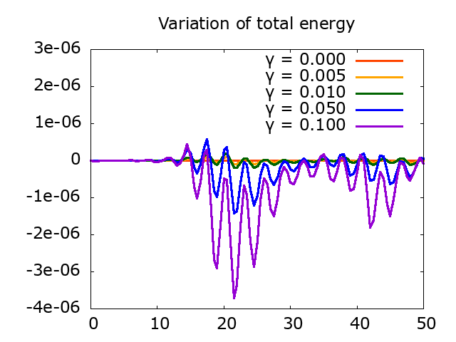
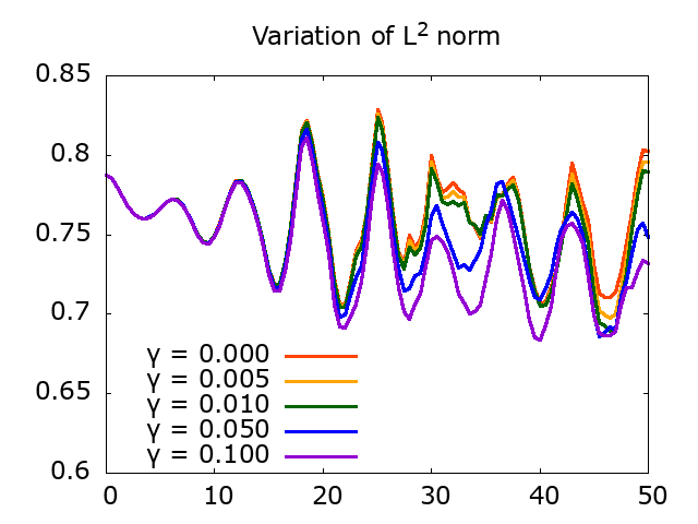
(a)	(b)
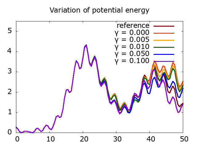
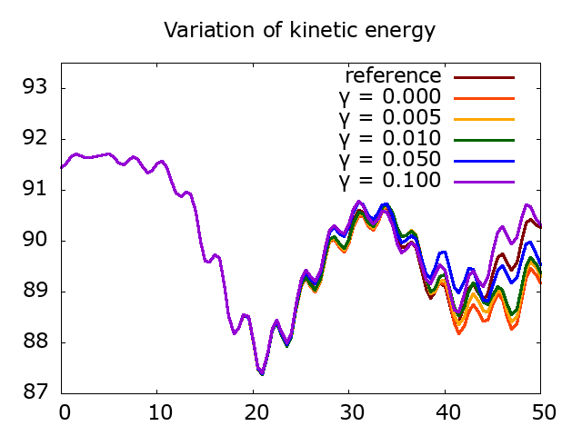
(c)	(d)

Figure 5.1. Test 2: time evolution of (a) the variation of the total energy, (b) the standard $L^{2}$ norm of $f$, (c) the potential energy and (d) the kinetic energy for $\alpha$ given by (2.15), with several values of $\gamma=0,...\,,\,10^{-1}$.

Finally, in Figure 5.2, we present the time evolution of $\alpha$ and the corresponding weighted $L^{2}$ norm for different values of $\gamma$. Since the initial data $\alpha(0)$ is the same for our simulations, we know that when $\gamma\leq\gamma^{\prime}$, we have $\alpha_{\gamma^{\prime}}(t)\leq\alpha_{\gamma}(t)$ (since $\alpha_{\gamma^{\prime}}$ decays faster than $\alpha_{\gamma}$) and then

$$\|f(t)\|_{L^{2}(\operatorname{d}\mu_{t}^{\prime})}\leq\|f(t)\|_{L^{2}(\operatorname{d}\mu_{t})},$$

where $\mu_{t}^{\prime}$ represents the measure associated to $\alpha_{\gamma^{\prime}}(t)$. We also notice that when $\gamma$ increases, the weighted $L^{2}$ norm $\|f(t)\|_{L^{2}(\operatorname{d}\mu_{t})},$ grows slowly, which is consistent with our estimate (5.2). Moreover, for a fixed $\gamma$, the time evolution of $\|f(t)\|_{L^{2}(\operatorname{d}\mu_{t})}$ first follows the growth of the potential energy which is almost exponentially fast, but when nonlinear effects dominate, it starts to oscillate and is stabilized. This last numerical result illustrates that the estimate (5.2) is certainly not optimal for large time…

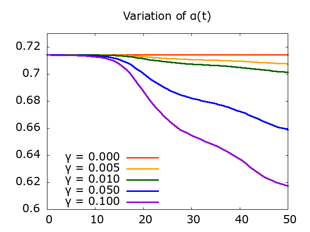
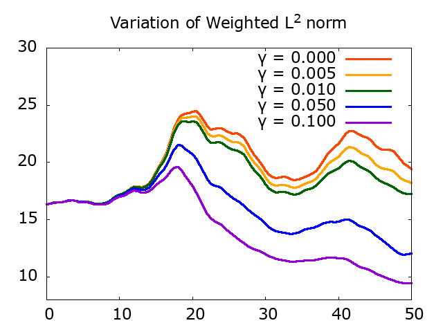
(a)	(b)

Figure 5.2. Test 2: time evolution of (a) the scaling function $\alpha$ and (b) the corresponding weighted $L^{2}$ norm of $f$, for $\alpha$ given by (2.15), with several values of $\gamma=0,...\,,\,10^{-1}$.

6. Conclusion & Perspectives

In this article we investigate the convergence analysis of a spectral Hermite discretization of the Vlasov-Poisson system with a time-dependent scaling factor allowing to prove the stability and convergence of the numerical solution in an appropriate functionnal framework. The control of this scaling factor, and more precisely a positive lower bound, is crucial to ensure completely the stability of the method and our proof follows carefully this dependency. Our analysis is limited to the one dimensional case for which the control of the electric field is straightforward. In a future work we would like to adapt our approach to the multi-dimensional case following the ideas in [3] for the control of the $L^{\infty}$ norm of the electric field in two and three dimensions.

References

- [1] T. P. Armstrong. Numerical studies of the nonlinear Vlasov equation. The Physics of Fluids, 10(6):1269–1280, 1967.
- [2] B. Ayuso, J. A. Carrillo, and C.-W. Shu. Discontinuous Galerkin methods for the one-dimensional Vlasov-Poisson system. Kinet. Relat. Models, 4(4):955–989, 2011.
- [3] B. Ayuso, J. A. Carrillo, and C.-W. Shu. Discontinuous Galerkin methods for the multi-dimensional Vlasov–Poisson problem. Mathematical Models and Methods in Applied Sciences, 22(12):1250042, 2012.
- [4] N. Besse. Convergence of a high-order semi-Lagrangian scheme with propagation of gradients for the one-dimensional Vlasov-Poisson system. SIAM J. Numer. Anal., 46(2):639–670, 2008.
- [5] M. Bessemoulin-Chatard and F. Filbet. On the stability of conservative discontinuous Galerkin/Hermite spectral methods for the Vlasov-Poisson system. Journal of Computational Physics, 451:110881, 2022.
- [6] C. K. Birdsall and A. B. Langdon. Plasma physics via computer simulation. McGraw-Hill, New York, 1985.
- [7] E. Camporeale, G. Delzanno, B. Bergen, and J. Moulton. On the velocity space discretization for the Vlasov–Poisson system: Comparison between implicit Hermite spectral and Particle-in-Cell methods. Computer Physics Communications, 198:47–58, 2016.
- [8] F. Charles, B. Després, and M. Mehrenberger. Enhanced convergence estimates for semi-Lagrangian schemes: application to the Vlasov-Poisson equation. SIAM J. Numer. Anal., 51(2):840–863, 2013.
- [9] Y. Cheng, I. M. Gamba, and P. J. Morrison. Study of conservation and recurrence of Runge–Kutta discontinuous Galerkin schemes for Vlasov–Poisson systems. Journal of Scientific Computing, 56(2):319–349, 2013.
- [10] Y. Di, Y. Fan, Z. Kou, R. Li, and Y. Wang. Filtered Hyperbolic Moment Method for the Vlasov Equation. Journal of Scientific Computing, 79(2):969–991, 2019.
- [11] R. Duclous, B. Dubroca, F. Filbet, and V. Tikhonchuk. High order resolution of the Maxwell–Fokker–Planck–Landau model intended for ICF applications. Journal of Computational Physics, 228(14):5072–5100, 2009.
- [12] F. Engelmann, M. Feix, E. Minardi, and J. Oxenius. Nonlinear effects from Vlasov’s equation. The Physics of Fluids, 6(2):266–275, 1963.
- [13] F. Filbet. Convergence of a finite volume scheme for the Vlasov-Poisson system. SIAM J. Numer. Anal., 39(4):1146–1169, 2001.
- [14] F. Filbet and E. Sonnendrücker. Comparison of Eulerian Vlasov solvers. Comput. Phys. Comm., 150(3):247–266, 2003.
- [15] F. Filbet and E. Sonnendrücker. Modeling and numerical simulation of space charge dominated beams in the paraxial approximation. Mathematical Models and Methods in Applied Sciences, 16(05):763–791, 2006.
- [16] F. Filbet and T. Xiong. Conservative Discontinuous Galerkin/Hermite Spectral Method for the Vlasov–Poisson System. Commun. Appl. Math. Comput., 2020.
- [17] J. C. M. Fok, B. Guo, and T. Tang. Combined Hermite spectral-finite difference method for the Fokker-Planck equation. Mathematics of computation, 71(240):1497–1528, 2001.
- [18] R. E. Heath, I. M. Gamba, P. J. Morrison, and C. Michler. A discontinuous Galerkin method for the Vlasov–Poisson system. Journal of Computational Physics, 231(4):1140–1174, 2012.
- [19] J. P. Holloway. Spectral velocity discretizations for the Vlasov-Maxwell equations. Transport theory and statistical physics, 25(1):1–32, 1996.
- [20] T. Y. Hou and R. Li. Computing nearly singular solutions using peseudo-spectral methods. Journal of Computational Physics, 226:379–397, 2007.
- [21] C. Johnson and J. Pitkäranta. An analysis of the discontinuous Galerkin method for a scalar hyperbolic equation. Mathematics of computation, 46(173):1–26, 1986.
- [22] G. Joyce, G. Knorr, and H. K. Meier. Numerical integration methods of the Vlasov equation. Journal of Computational Physics, 8(1):53–63, 1971.
- [23] A. J. Klimas and W. M. Farrell. A splitting algorithm for Vlasov simulation with filamentation filtration. J. Comput. Phys., 110(1):150–163, 1994.
- [24] K. Kormann and A. Yurova. A generalized Fourier–Hermite method for the Vlasov–Poisson system. BIT Numerical Mathematics, pages 1–29, 2021.
- [25] S. Le Bourdiec, F. De Vuyst, and L. Jacquet. Numerical solution of the Vlasov–Poisson system using generalized Hermite functions. Computer physics communications, 175(8):528–544, 2006.
- [26] P.-L. Lions and B. Perthame. Propagation of moments and regularity for the -dimensional Vlasov-Poisson system. Invent. Math., 105(2):415–430, 1991.
- [27] H. Ma, W. Sun, and T. Tang. Hermite spectral methods with a time-dependent scaling for parabolic equations in unbounded domains. SIAM journal on numerical analysis, 43(1):58–75, 2005.
- [28] H. Ma and T. Zhao. A stabilized Hermite spectral method for second-order differential equations in unbounded domains. Numerical Methods for Partial Differential Equations: An International Journal, 23(5):968–983, 2007.
- [29] G. Manzini, G. L. Delzanno, J. Vencels, and S. Markidis. A Legendre–Fourier spectral method with exact conservation laws for the Vlasov–Poisson system. Journal of Computational Physics, 317:82–107, 2016.
- [30] G. Manzini, D. Funaro, and G. L. Delzanno. Convergence of Spectral Discretizations of the Vlasov–Poisson System. SIAM Journal on Numerical Analysis, 55(5):2312–2335, 2017.
- [31] K. Pfaffelmoser. Global classical solutions of the Vlasov-Poisson system in three dimensions for general initial data. J. Differential Equations, 95(2):281–303, 1992.
- [32] J. W. Schumer and J. P. Holloway. Vlasov simulations using velocity-scaled Hermite representations. Journal of Computational Physics, 144(2):626–661, 1998.
- [33] M. Shoucri and G. Knorr. Numerical integration of the Vlasov equation. Journal of Computational Physics, 14(1):84–92, 1974.
- [34] J. W. Shumer and J. P. Holloway. Vlasov simulations using velocity-scaled Hermite representations. Journal of Computational Physics, 144(2):626–661, 1998.
- [35] E. Sonnendrücker, F. Filbet, A. Friedman, E. Oudet, and J.-L. Vay. Vlasov simulations of beams with a moving grid. Computer Physics Communications, 164(1-3):390–395, 2004.
- [36] E. Sonnendrücker, J. Roche, P. Bertrand, and A. Ghizzo. The semi-Lagrangian method for the numerical resolution of the Vlasov equation. Journal of Computational Physics, 149(2):201–220, 1999.
- [37] T. Tang. The Hermite spectral method for Gaussian-type functions. SIAM journal on scientific computing, 14(3):594–606, 1993.
- [38] S. Ukai and T. Okabe. On classical solutions in the large in time of two-dimensional Vlasov’s equation. Osaka Math. J., 15(2):245–261, 1978.
- [39] C. Yang and M. Mehrenberger. Highly accurate monotonicity-preserving semi-Lagrangian scheme for Vlasov-Poisson simulations. J. Comput. Phys., 446:Paper No. 110632, 33, 2021.
- [40] S. Zaki, L. Gardner, and T. Boyd. A finite element code for the simulation of one-dimensional Vlasov plasmas. I. Theory. Journal of Computational Physics, 79(1):184–199, 1988.
- [41] S. I. Zaki, T. Boyd, and L. Gardner. A finite element code for the simulation of one-dimensional Vlasov plasmas. II. Applications. Journal of Computational Physics, 79(1):200–208, 1988.