The Kähler geometry of toric manifolds

Preface

These notes are written for a mini-course I gave at the CIRM in Luminy in 2019. Their intended purpose was to present, in the context of smooth toric varieties, a relatively self-contained and elementary introduction to the theory of extremal Kähler metrics pioneered by E. Calabi in the 1980’s and extensively developed in recent years. The framework of toric varieties, used in both symplectic and algebraic geometry, offers a fertile testing ground for the general theory of extremal Kähler metrics and provides an important class of smooth complex varieties for which the existence theory is now understood in terms of a stability condition of the corresponding Delzant polytope. The notes do not contain any original material nor do they take into account some more recent developments, such as the non-Archimedean approach to the Calabi problem. I’m making them available on the arXiv because I continue to get questions about how they can be cited.

Acknowledgements

I am grateful to Éveline Legendre, Alexandro Lepé, Simon Jubert, Lars Sektnan, Isaque Viza de Souza, and Yicao Wang for their careful reading of previous versions of the manuscript, spotting and correcting typos and errors, and suggesting improvements. I have benefited from numerous discussions with Paul Gauduchon, Éveline Legendre and Lars Sektnan during the preparation of the notes. Special thanks are due to David Calderbank for his collaborations on the topic and for kindly allowing me to reproduce his elegant (unpublished) proof of Proposition 3.3.

Chapter 1 Delzant Theory

1.1. Hamiltonian group actions on symplectic manifolds

We start with some basic definitions in symplectic geometry.

Let $(M^{2m},\omega)$ be a symplectic manifold of real dimension $2m$, i.e. a smooth manifold endowed with a closed $2$-form $\omega$ which is non-degenerate at each point $p\in M$ meaning that $\omega_{p}:T_{p}M\to T^{*}_{p}M$ is an isomorphism. A simple linear algebra shows that the latter condition is also equivalent to $\omega_{p}^{\wedge m}\neq 0\in\wedge^{2m}(T^{*}_{p}M).$

Example 1.1.

The basic example of a symplectic manifold is $({\mathbb{R}}^{2m},\omega_{0})$ where, using the identification

$${\mathbb{R}}^{2m}\cong{\mathbb{C}}^{m}=\{z=(z_{1},\cdots,z_{m}):z_{i}=x_{i}+\sqrt{-1}y_{i},i=1,\ldots m\},$$

the symplectic form is

$$\omega_{0}:=\sum_{i=1}^{m}dx_{i}\wedge dy_{i}=\frac{\sqrt{-1}}{2}\sum_{i=1}^{n}dz_{i}\wedge d\bar{z}_{i}.$$

Example 1.2.

Let $M={\mathbb{S}}^{2}\subset{\mathbb{R}}^{3}$ be the unit sphere endowed with the atlas of ${\mathbb{S}}^{2}$ given by the stereographic projections from the north and the south poles, $N=(0,0,1)$ and $S=(0,0,-1)$, respectively. We denote by

$$\begin{split}x&=\frac{2u}{1+u^{2}+v^{2}},y=\frac{2v}{1+u^{2}+v^{2}},z=-\frac{1-u^{2}-v^{2}}{1+u^{2}+v^{2}},\ (u,v)\in{\mathbb{R}}^{2},\\ x&=\frac{2\tilde{u}}{1+\tilde{u}^{2}+\tilde{v}^{2}},y=\frac{2\tilde{v}}{1+\tilde{u}^{2}+\tilde{v}^{2}},z=\frac{1-\tilde{u}^{2}-\tilde{v}^{2}}{1+\tilde{u}^{2}+\tilde{v}^{2}},\ (\tilde{u},\tilde{v})\in{\mathbb{R}}^{2}\end{split}$$

the corresponding chart patches on ${\mathbb{S}}^{2}$. Recall that on ${\mathbb{S}}^{2}\setminus(\{N\}\cup\{S\})$, the transition between the coordiantes $(u,v)$ and $(\tilde{u},\tilde{v})$ is given by the diffeomorphism $\tilde{u}=\frac{u}{u^{2}+v^{2}},\tilde{v}=\frac{v}{u^{2}+v^{2}}$ of ${\mathbb{R}}^{2}\setminus\{(0,0)\}$. Then the $2$-form

$$\omega_{{\mathbb{S}}^{2}}:=\frac{4du\wedge dv}{(1+u^{2}+v^{2})^{2}}=-\frac{4d\tilde{u}\wedge d\tilde{v}}{(1+\tilde{u}^{2}+\tilde{v}^{2})^{2}}$$

introduces a symplectic structure on ${\mathbb{S}}^{2}$.

Definition 1.1.

Let $M$ be a smooth manifold and $G$ a Lie group. An action of $G$ on $M$ is a group homomorphism

$$\rho:G\to{\rm Diff}(M),$$

where ${\rm Diff}(M)$ stands for the diffeomorphism group of $M$. The action of $G$ is smooth if the evaluation map

$${\rm ev}:G\times M\to M,\ \ {\rm ev}(g,p):=\rho(g)(p),$$

is a smooth map between manifolds.

Let $(M,\omega)$ be a symplectic manifold and $G$ a Lie group acting smoothly on $M$. We say that $G$ acts symplectically on $(M,\omega)$ if

$$\rho(g)^{*}(\omega)=\omega.$$

Example 1.3.

Consider $(M,\omega)=({\mathbb{R}}^{2m},\omega_{0})$ as in Example 1.1. The action of the $m$-dimensional torus

$${\mathbb{T}}^{m}=(e^{\sqrt{-1}t_{1}},\ldots,e^{\sqrt{-1}t_{m}}),$$

given by

$$\rho(e^{\sqrt{-1}t_{1}},\ldots,e^{\sqrt{-1}t_{m}})(z):=(e^{\sqrt{-1}t_{1}}z_{1},\ldots,e^{\sqrt{-1}t_{m}}z_{m})$$

is symplectic.

Example 1.4 (Hamiltonian flows).

Let $f$ be a smooth function on $(M,\omega)$. Using the non-degeneracy of $\omega$, we define a vector field by

$$X_{f}:=-\omega^{-1}(df),$$

called the Hamiltonian vector field of $f$. Suppose that $X_{f}$ is complete, i.e. its flow $\varphi_{t}$ is defined for all $t\in{\mathbb{R}}$ (this always holds if $M$ is compact). Then, $\rho(t):=\varphi_{t}$ defines a symplectic action of ${\mathbb{R}}$ on $(M,\omega)$. Indeed, we have

$$\begin{split}\frac{d}{dt}_{|_{t=s}}(\varphi_{t}^{*}\omega)&=\varphi_{s}^{*}\Big{(}\frac{d}{dt}_{|_{t=0}}(\varphi^{*}_{t}\omega)\Big{)}\\ &=\varphi_{s}^{*}\Big{(}{\mathcal{L}}_{X_{f}}\omega\Big{)}\\ &=\varphi_{s}^{*}\Big{(}d\imath_{X_{f}}+\imath_{X_{f}}d)(\omega)\Big{)}\\ &=\varphi_{s}^{*}\Big{(}d(-df)\Big{)}=0,\\ \varphi_{0}^{*}(\omega)&=\omega.\end{split}$$

The previous two examples show that different groups (in particular ${\mathbb{T}}^{m}$ and ${\mathbb{R}}^{m}$) can possibly give rise to “equivalent” symplectic actions, in the sense that their images in ${\rm Diff}(M)$ are the same. A way to normalize the situation is to consider

Definition 1.2.

A symplectic action of a Lie group $G$ on $(M,\omega)$ is effective if the homomorphism $\rho:G\to{\rm Diff}(M)$ has trivial kernel.

Thus, the symplectic action of ${\mathbb{R}}^{m}=\{(t_{1},\ldots,t_{m})\}$ on $({\mathbb{R}}^{2m},\omega_{0})$ defined in Example 1.3 is not effective, whereas the action of ${\mathbb{T}}^{m}$ on the same manifold is. In the sequel, we shall be interested in effective symplectic actions.

Let $G$ be a Lie group acting smoothly on $M$. Denote by $\mathfrak{g}={\rm Lie}(G)$ its Lie algebra, i.e. $\mathfrak{g}$ is the vector space of left-invariant vector fields on $G$. For any $\xi\in\mathfrak{g}$, we denote by ${\rm exp}(t\xi)$ the corresponding 1-parameter subgroup of $G,$ and by $X_{\xi}$ the vector field on $M$ induced by the one parameter subgroup $\rho(\exp(t\xi))$ in ${\rm Diff}(M)$, i.e.

$$X_{\xi}(p):=\frac{d}{dt}_{|_{t=0}}\Big{(}\rho(\exp(t\xi))(p)\Big{)}.$$

The vector field $X_{\xi}$ is called fundamental vector field of $\xi\in\mathfrak{g}$.

We recall that $G$ also acts on itself by conjugation

$$\rho(g)(h):=ghg^{-1},\ \ g\in G,h\in G,$$

fixing the unitary element $e\in G$ and thus inducing a linear action on the vector space $T_{e}G\cong\mathfrak{g}$, called the adjoint action

$${\rm Ad}:G\to{\bf GL}(\mathfrak{g}).$$

The induced linear action on the dual vector space $T^{*}_{e}G\cong\mathfrak{g}^{*}$ is given by ${\rm Ad}^{*}(g)(\alpha):=\alpha\circ{\rm Ad}(g^{-1})$ and is called the co-adjoint action. We are now ready to give the definition of a hamiltonian action on $(M,\omega)$.

Definition 1.3.

Let $\rho:G\to{\rm Diff}(M)$ be a smooth action of a Lie group $G$ on $(M,\omega)$. It is said to be hamiltonian if there exists a smooth map

$$\mu:M\to\mathfrak{g}^{*},$$

called a momentum map, which satisfies the following two conditions.

1. For any $\xi\in\mathfrak{g}$, the fundamental vector field $X_{\xi}$ satisfies

   $$\omega(X_{\xi},\cdot)=-d\langle\mu,\xi\rangle,$$

   where $\langle\cdot,\cdot\rangle$ denotes the natural pairing between $\mathfrak{g}$ and its dual $\mathfrak{g}^{*}$.

2. $\mu$ is equivariant with respect to the action $\rho$ of $G$ on $M$ and the co-adjoint action ${\rm Ad}^{*}$ of $G$ on $\mathfrak{g}^{*}$, i.e.

   $$\mu\big{(}\rho(g)(p)\big{)}={\rm Ad}^{*}(g)\big{(}\mu(p)\big{)}.$$

Remark 1.1.

(a) Notice that the condition (i) of Definition 1.3 implies that any fundamental vector field $X_{\xi}$ is hamiltonian (see Example 1.4) with respect to the smooth function

(1.1) $$\mu_{\xi}(p):=\langle\mu(p),\xi\rangle.$$

In particular, hamiltonian actions are symplectic.

(b) By a standard argument in Lie theory, the condition (ii) of Definition 1.3 can be equivalently expressed as

$$d\mu_{\xi}(X_{\eta})=-\mu_{[\eta,\xi]}.$$

For any two smooth functions $f,h$ on $(M,\omega)$

$$\{f,h\}_{\omega}:=\omega(X_{f},X_{h})$$

is the so-called Poisson bracket. Thus, the condition (ii) of Definition 1.3 is equivalent to

(1.2) $$\{\mu_{\xi},\mu_{\eta}\}_{\omega}=-\mu_{[\xi,\eta]}.$$

An important example is the following

Example 1.5.

Suppose $G$ is a semi-simple compact Lie group with Lie algebra $\mathfrak{g}$, and ${\mathbb{T}}\subset G$ is a maximal torus with Lie algebra $\mathfrak{t}\subset\mathfrak{g}$. Complexifying, we also have a semi-simple complex Lie group $G^{{\mathbb{C}}}$ with Lie algebra $\mathfrak{g}^{c}{{\mathbb{C}}}:=\mathfrak{g}\otimes{\mathbb{C}}$, and a Cartan sub-algebra $\mathfrak{h}:=\mathfrak{t}\otimes{\mathbb{C}}$. A specific example which one can bear in mind is $G={\bf SU}(n)$, ${\mathbb{T}}=\{{\rm diag}(e^{\sqrt{-1}t_{1}},\ldots,e^{\sqrt{-1}t_{m}}):t_{1}+\cdots+t_{m}=0\}$. Then $G^{{\mathbb{C}}}={\bf SL}(n,{\mathbb{C}})$.

The general theory of semi-simple Lie algebras yields that $\mathfrak{g}^{{\mathbb{C}}}$ admits a root decomposition

$$\mathfrak{g}^{{\mathbb{C}}}=\mathfrak{h}\oplus\bigoplus_{\alpha\in R_{+}}(\mathfrak{g}^{{\mathbb{C}}}_{-\alpha}\oplus\mathfrak{g}^{{\mathbb{C}}}_{\alpha}),$$

where $R\subset\mathfrak{h}^{*}$ denotes the finite subspace of roots of $\mathfrak{g}^{{\mathbb{C}}}$ and $R=R_{+}\cup(-R_{+})$ with $R_{+}\cap(-R_{+})=\emptyset$ is the choice of a subset $R_{+}$ of positive roots. For $\alpha\in R$, we have set

$$\mathfrak{g}^{{\mathbb{C}}}_{\alpha}:=\{u\in\mathfrak{g}^{{\mathbb{C}}}:{\rm ad}_{x}(u)=\alpha(x)u,\ \forall x\in\mathfrak{h}\}.$$

We denote by $M$ an orbit in $\mathfrak{g}$ for the adjoint action ${\rm Ad}:G\to{\bf GL}(\mathfrak{g})$ and assume that $M$ is not a point. The general theory tells us that $M$ is aways the orbit of a non-zero element $x\in\mathfrak{t}$, and that such $x$ is unique if we require moreover that $-i\alpha(x)\geq 0$ for all $\alpha\in R_{+}$. If the unique $x\in\mathfrak{t}$ determined as above also satisfies $-i\alpha(x)>0$ for all $\alpha\in R_{+}$, then the orbit $M\cong G/{\mathbb{T}}$ is principal for the adjoint action of $G$, and $M$ is called a flag manifold. In general, $M\cong G/G_{x}$ where $G_{x}$ is the subgroup of $G$ fixing $x$ (and whose Lie algebra is $\mathfrak{g}_{x}={\rm Ker}({\rm ad}_{x})$).

In the case $G={\bf SU}(n),$ this corresponds to the basic fact that any hermitian matrix $a\in\sqrt{-1}{\bf su}(n,{\mathbb{C}})$ can be diagonalized by a conjugation with an element of ${\bf SU}(n)$. The diagonal matrix is uniquely determined up to a permutation of its (real) eigenvalues, so we can normalize it by ordering the eigenvalues in decreasing order. A hermitian matrix $a$ determines a regular orbit for the action of $G={\bf SU}(n)$ by conjugation precisely when $a$ has simple spectrum.

Each orbit $M$ admits a natural symplectic form $\omega$, called the Kirillov–Kostant–Souriau form, whose definition we now recall. As the tangent space $T_{y}M$ for any $y\in M$ is generated by the fundamental vector fields for the adjoint action of $G$, $T_{y}M$ can be identified with the image $\mathfrak{m}_{y}\subset\mathfrak{g}$ of the map

(1.3) $$u\to\frac{d}{dt}_{|_{t=0}}{\rm Ad}_{\exp(tu)}(y)=-{\rm ad}_{y}(u).$$

For $u,v\in\mathfrak{g}$, we denote by

$$\langle u,v\rangle:={\rm tr}(ad_{u}\circ ad_{v})$$

the Killing form of $\mathfrak{g}$. By assumption $\langle\cdot,\cdot\rangle$ is negative definite ($G$ being compact and semi-simple). We then set

$$\omega_{y}(u,v):=-\langle y,[u,v]\rangle,$$

where $u,v\in T_{y}M\cong{\rm Im}({\rm ad}_{y})$. Then $\omega$ gives rise to a symplectic structure on $M=G/G_{x}$. The main fact is

Proposition 1.1 (Kirillov–Kostant–Souriau).

The 2-form $\omega$ defines a symplectic structure on $M=G/G_{x}$, the adjoint action of $G$ on $(M,\omega)$ is hamiltonian with momentum map $\mu:M\to\mathfrak{g^{*}}$ identified with the inclusion $\imath:M\subset\mathfrak{g}$ composed with the Killing form $\langle\cdot,\cdot\rangle:\mathfrak{g}\to\mathfrak{g}^{*}.$

1.2. Hamiltonian actions of tori

We now specialize to the case when the Lie group $G={\mathbb{T}}^{k}$ is a $k$-dimensional torus.

Lemma 1.1.

Suppose $G={\mathbb{T}}^{k}$ acts symplectically on $(M,\omega)$. Then, the action is hamiltonian if and only if for any $\xi\in\mathfrak{g}$, there exists a smooth function $\mu_{\xi}$ on $M$, such that $\imath_{X_{\xi}}\omega=-d\mu_{\xi}$. In this case, the momentum map $\mu:M\to\mathfrak{g}^{*}$ is determined up to the addition of a vector in $\mathfrak{g}^{*}$.

Proof.

If the action of $G$ is hamiltonian, the existence of $\mu_{\xi}$ follows from Remark 1.1(a).

Conversely, suppose that each fundamental vector field $X_{\xi}$ is hamiltonian with respect to a smooth function $\mu_{\xi}$ on $M$. Choose a basis $\{\xi_{1},\ldots,\xi_{k}\}$ of $\mathfrak{g}$ and let $X_{1},\ldots,X_{k}$ and $\mu_{1},\ldots,\mu_{k}$ be the corresponding fundamental vector fields and hamiltonian function, respectively. We claim that for $\xi=\sum_{i=1}^{k}a_{i}\xi_{i}$, the function

(1.4) $$\mu_{\xi}:=\sum_{i=1}^{k}a_{i}\mu_{i}$$

is a hamiltonian of the induced fundamental vector field $X_{\xi}$. Indeed, since $G$ is abelian, $\exp(t\xi)=\exp(ta_{1}\xi_{1})\circ\cdots\circ\exp(ta_{k}\xi_{k})$ and, therefore, the induced fundamental vector field is $X_{\xi}=\sum_{i=1}^{k}a_{i}X_{\xi_{i}}$. The claim then follows trivially. Thus, we can define $\mu:M\to\mathfrak{g}^{*}$ by letting

$$\langle\mu(p),\xi\rangle:=\mu_{\xi}.$$

It remains to show that the condition (1.2) holds. As the co-adjoint action of an abelian group $G$ is trivial, this condition reduces to show that $\mu_{\xi}$ is an invariant function under the action of $G$. Equivalently, by Remark 1.1(b), we have to show that for any fundamental vector fields $X_{\xi},X_{\eta}$, the smooth function $\{\mu_{\xi},\mu_{\eta}\}_{\omega}=\omega(X_{\xi},X_{\eta})$ identically vanishes on $M$. Since the action of $G$ is symplectic, for any fundamental vector field $X_{\zeta},$ $\mathcal{L}_{X_{\zeta}}\omega=0$. It follows (by using that $G$ is abelian again) that $\mathcal{L}_{X_{\zeta}}(\omega(X_{\xi},X_{\eta}))=0$. Thus, $\omega(X_{\xi},X_{\eta})$ is a constant function on each orbit $\mathcal{O}\subset M$ for the action of $G$ on $M$. It is a standard fact that $\mathcal{O}$ is a homogeneous manifold $G/G_{p},$ where $p\in\mathcal{O}$ and $G_{p}$ is the stabilizer of $p$ in $G$, see e.g. [5]. As $G$ is compact, $\mathcal{O}$ is a compact manifold (see [5], Chapter 1, Corollary 1.3), and therefore the restriction of $\mu_{\xi}$ to $\mathcal{O}$ has a critical point. At this point, $\omega(X_{\xi},X_{\eta})=-d\mu_{\xi}(X_{\eta})=0$, thus showing that the function $\omega(X_{\xi},X_{\eta})$ is identically zero on $\mathcal{O}$, and hence on $M$.

The last statement trivially follows as we can take instead of $\mu_{i}$ the hamiltonian $\mu_{i}+\lambda_{i}$ with $\lambda_{i}\in{\mathbb{R}}$ or, equivalently, we can replace in (1.4) $\mu_{\xi}$ by $\mu_{\xi}+\langle\xi,\lambda\rangle$ for $\lambda\in\mathfrak{g}^{*}$. ∎

For the next result, we use the facts that if a compact Lie group $G$ acts effectively on $M$, then each orbit $\mathcal{O}=G(p)$ is a compact homogeneous manifold of dimension $\leq\dim G$ and, furthermore, that there exist an open dense subset $M^{0}\subset M$ of points whose orbits are of dimension $=\dim G$ (called principal orbits of $G$). We refer to [5] for a proof of these facts.

Lemma 1.2.

Suppose that $(M^{2m},\omega)$ admits an effective hamiltonian action of $G={\mathbb{T}}^{k}$. Then $k\leq m$.

Proof.

By the argument in the proof of Lemma 1.1, the tangent space $T_{p}\mathcal{O}$ of a principal orbit $\mathcal{O}=G(p)$ is $\omega_{p}$ isotropic subspace of $T_{p}M$. Its dimension ($=\dim G$), therefore, is $\leq m$. ∎

Example 1.6.

We return again to Example 1.3 and will now show that the symplectic action of ${\mathbb{T}}^{m}$ on $({\mathbb{R}}^{2m},\omega_{0})$ is hamiltonian. We shall work on the dense open subset $({\mathbb{C}}^{m})^{0}=\{(z_{1},\ldots,z_{m}):z_{i}\neq 0,\ \forall i=1,\ldots m\}$ of ${\mathbb{C}}^{m}\cong{\mathbb{R}}^{2m}$ on which we introduce polar coordinates $z_{i}=r_{i}e^{\sqrt{-1}\varphi_{i}},i=1,\ldots,m$. The symplectic $2$-form $\omega_{0}$ then becomes

$$\omega_{0}=\sum_{i=1}^{m}r_{i}dr_{i}\wedge d\varphi_{i},$$

whereas the fundamental vector fields $\{X_{1},\ldots,X_{m}\}$ associated to the standard basis of ${\mathbb{R}}^{m}=\{(t_{1},\ldots,t_{m})\}\cong{\rm Lie}({\mathbb{T}}^{m})$ are $X_{i}=\frac{\partial}{\partial\varphi_{i}}.$ It follows that $\imath_{X_{i}}\omega_{0}=-r_{i}dr_{i}=-d(\frac{1}{2}r_{i}^{2}).$ In other words, the smooth map $\mu:{\mathbb{C}}^{m}\to{\mathbb{R}}^{m}\cong\Big{(}{\rm Lie}({\mathbb{T}}^{m})\Big{)}^{*}$ defined by

(1.5) $$\mu(z):=\frac{1}{2}\big{(}|z_{1}|^{2},\ldots,|z_{m}|^{2}\big{)}$$

is a momentum map for the action of ${\mathbb{T}}^{m}$ on $({\mathbb{C}}^{m})^{0}$, and hence on ${\mathbb{C}}^{m}$ (by continuity). We also notice that

(1.6) $${\rm Im}(\mu)=C_{m}:=\{(x_{1},\ldots,x_{m})\in{\mathbb{R}}^{m}:x_{i}\geq 0\}.$$

Exercise 1.1.

Consider the ${\mathbb{S}}^{1}$-action on $({\mathbb{S}}^{2},\omega_{{\mathbb{S}}^{2}})$ corresponding to the rotation around the $z$-axis of ${\mathbb{R}}^{3}$, see Example 1.2. Show that this is hamiltonian with momentum map given by the $z$-ccordinate.

The central result in the theory is the following convexity result

Theorem 1.1 (Atiyah [4], Guillemin–Stenberg [27]).

Suppose ${\mathbb{T}}^{k}$ acts in a hamiltonian way on a connected compact symplectic manifold $(M,\omega)$, with momentum map $\mu:M\mapsto{\mathbb{R}}^{k}$. Then,

1. The image of $\mu$ is the convex hull $\Delta\subset{\mathbb{R}}^{k}$ of the images of the fixed points for the ${\mathbb{T}}^{k}$-action on $M$.

2. The pre-image of any point of $\Delta$ is connected.

Example 1.7 (Schür’s Theorem).

This is the main application of Theorem 1.1 given in [4]. In the general setting of Example 1.5, let us take $G={\bf SU}(n)$ and consider the orbit $M=M_{a}$ of all conjugated hermitian matrices to a given hermitian matrix $a$ by elements of $G$. We thus have a hamiltonian action on $(M,\omega)$ of the $(n-1)$-dimensional torus ${\mathbb{T}}\subset{\bf SU}(n)$ of diagonal matrices in ${\bf SU}(n)$. Furthermore, it easily follows by Proposition 1.1 that the momentum map for this action is

$$\mu(b)={\rm diag}(b_{11},\ldots,b_{nn}),$$

where $b$ is any hermitian matrix in $M_{a}$ and $(b_{11},\ldots,b_{nn})$ are the diagonal elements of $b$ (a vector in ${\mathbb{R}}^{n}$). Furthermore, the fixed points for the action of ${\mathbb{T}}$ on $M_{a}$ are precisely the diagonal hermitian matrices in $M_{a}$. We thus obtain from Theorem 1.1 the following classical result due to Schür.

Corollary 1.2.1.

Let $a$ be a hermitian matrix in ${\mathbb{C}}^{n}$ with spectrum $(\lambda_{1},\ldots,\lambda_{n})\in{\mathbb{R}}^{n}$. Then the diagonal elements of the hermitian matrices in the conjugacy class of $a$ by elements of ${\bf U}(n)$ consisting of all points in the convex hull in ${\mathbb{R}}^{n}$ of $\{(\lambda_{\sigma(1)},\ldots,\lambda_{\sigma(n)}),\sigma\in S_{n}\},$ where $S_{n}$ denotes the symmetric group of permutation of $n$-elements.

1.2.1. Toric symplectic manifolds and Delzant Theorem

In view of Lemma 1.2, we give the following

Definition 1.4.

A symplectic toric manifold is a compact connected symplectic manifold $(M^{2m},\omega)$ endowed with an effective hamiltonian action $\rho$ of a torus ${\mathbb{T}}$ with

$${\rm dim}\ {\mathbb{T}}=m=\frac{1}{2}{\rm dim}\ M.$$

Two toric symplectic manifolds $(M_{i},\omega_{i},{\mathbb{T}}_{i},\rho_{i}),i=1,2$ are considered equivalent if there exist an isomorphism of Lie groups $\phi:{\mathbb{T}}_{1}\to{\mathbb{T}}_{2}$ and a diffeomorphism $\Phi:M_{1}\to M_{2}$ with $\Phi^{*}\omega_{2}=\omega_{1}$, satisfying

$$\Phi(\rho_{1}(g)(p))=\rho_{2}(\phi(g))(\Phi(p)),\ \forall g\in{\mathbb{T}}_{1},\ \forall\ p\in M_{1}.$$

By Lemma 1.1, we can always assume that in this case the momentum maps $\mu_{i}$ of $(M_{i},\omega_{i},{\mathbb{T}}_{i},\rho_{i})$ are linked by $\mu_{1}=\mu_{2}\circ\Phi$.

By virtue of Theorem 1.1, the image of a toric symplectic manifold of dimension $2m$ is a compact convex polytope $\Delta$ in the $m$-dimensional vector space $\mathfrak{t}^{*}={\rm Lie}({\mathbb{T}})$. The Delzant theorem provides a classification (up to the equivalence of Definition 1.4) of symplectic toric manifolds $(M,\omega,{\mathbb{T}})$ in terms of the corresponding polytopes $\Delta\subset\mathfrak{t}^{*}$. To state it properly, we notice that being Lie algebra of a torus ${\mathbb{T}}$, the vector space $\mathfrak{t}$ comes equipped with a lattice $\Lambda\subset\mathfrak{t}$ such that $2\pi\Lambda={\rm exp}^{-1}(e)$ (where $e$ stands for the identity element of ${\mathbb{T}}$). In other words,

$$\exp:{\mathfrak{t}}/{2\pi\Lambda}\cong{\mathbb{T}}.$$

Definition 1.5.

Let $V$ be an $m$-dimensional real vector space whose dual space is $V^{*}$, and let $\Lambda\subset V$ be a lattice. We denote also by $V^{*}$ the affine space determined by $V^{*}$. Let $\Delta\subset V^{*}$ be a convex polytope written as the intersection of a minimal number of $d$ linear inequalities

$$\Delta=\{x\in V^{*}:L_{j}(x)=\langle u_{j},x\rangle+\lambda_{j}\geq 0,j=1,\ldots,d\},$$

where $u_{j}\in V$ are called (labelled) normals of $\Delta$ and $\lambda_{j}\in{\mathbb{R}}$. We shall refer to the collection ${\bf L}=\{L^{1},\ldots,L_{d}\}$ of affine-linear functions defining $\Delta$ as a labelling of $\Delta$, and to the couple $(\Delta,{\bf L})$ as a labelled polytope in $V$. We say that the data $(\Delta,{\bf L},\Lambda)$ define a Delzant polytope if the following conditions are satisfied:

1. $\Delta$ is compact;

2. $\Delta$ is simple, meaning that each vertex $x_{0}$ of $\Delta$ annihilates precisely $m$ of the affine functions in ${\bf L}$ and the corresponding normals form a basis of $V$;

3. $\Delta$ is integral, meaning that for each vertex $x_{0}$ of $\Delta$,

   $${\rm span}_{{\mathbb{Z}}}\{u_{j}\in V:L_{j}(x_{0})=\langle u_{j},x_{0}\rangle+\lambda_{j}=0\}=\Lambda.$$

We say that $(\Delta,{\bf L},\Lambda)$ defines a rational Delzant polytope if instead of (iii) we require the weaker assumption

1. $\Delta$ is rational, meaning that for each $L_{j}\in{\bf L}$, the normal $u_{j}\in\Lambda$.

Exercise 1.2.

Show that if the triple $(\Delta,{\bf L},\Lambda)$ is a Delzant polytope, then $(\Delta,\Lambda)$ determine the labelling ${\bf L}$. Is this true for a rational Delzant polytope $(\Delta,{\bf L},\Lambda)$?

Theorem 1.2 (Delzant [15]).

There exists a bijective correspondence between the equivalence classes of 2m-dimensional toric symplectic manifolds and equivalent Delzant polytopes $(\Delta,{\bf L},\Lambda)$ in an $m$-dimensional vector space $V^{*}$, up to the natural action of the affine group ${\rm Aff}(V^{*})$ on the triples $(\Delta,{\bf L},\Lambda)$.

We shall not develop in these notes a detailed proof of this key result, but in the next section we are going to sketch one direction of it, namely the Delzant construction which associates to a Delzant triple $(\Delta,{\bf L},\Lambda)$ a toric symplectic manifold $(M,\omega,{\mathbb{T}})$.

1.3. The complex projective space

We start with the following basic example of a toric symplectic manifold.

Recall that the (complex) $m$-dimensional projective space

$${\mathbb{C}}P^{m}={\mathbb{C}}^{m+1}\setminus\{0\}/{\mathbb{C}}^{*}$$

is the quotient of ${\mathbb{C}}^{m+1}\setminus\{0\}$ by the diagonal (holomorphic) action of ${\mathbb{C}}^{*}$ given by

$$(\lambda,z)\to\lambda z,\ \lambda\in{\mathbb{C}}^{*},\ z\in{\mathbb{C}}^{m+1}\setminus\{0\}.$$

This description naturally realizes $M={\mathbb{C}}P^{m}$ as a complex manifold, by passing from the homogenous coordinates $[z_{0},\ldots,z_{m}]$ (where $(z_{0},\ldots,z_{m})\in{\mathbb{C}}^{m+1}\setminus\{0\}$ and $[z_{0},\ldots,z_{m}]$ stands for the equivalence under the diagonal action of ${\mathbb{C}}^{*}$) to the affine charts $U_{i}\cong{\mathbb{C}}^{m}$ on the open subsets of ${\mathbb{C}}P^{m}$ where $z_{i}\neq 0.$ In order to describe the Fubini–Study metric on ${\mathbb{C}}P^{m}$, or its symplectic form, it is more convenient to consider the identification

$${\mathbb{C}}P^{m}={\mathbb{S}}^{2m+1}/{\mathbb{S}}^{1},$$

where ${\mathbb{S}}^{2m+1}\subset{\mathbb{C}}^{m+1}$ is the unit sphere with respect to the standard euclidean product of ${\mathbb{R}}^{2m+2}\cong{\mathbb{C}}^{m+1},$ and ${\mathbb{S}}^{1}$ denotes the diagonal circle action on ${\mathbb{S}}^{2m+1}\subset{\mathbb{C}}^{m+1}$ by

(1.7) $$\rho(e^{\sqrt{-1}t})(z_{0},\ldots,z_{m})=e^{\sqrt{-1}t}(z_{0},\ldots,z_{m}).$$

Definition 1.6.

Let $(M,\omega)$ be a symplectic manifold. An $\omega$-compatible riemannian metric $g$ on $M$ is a riemannian metric such that the field of endomorphisms $J$ defined by

$$g_{p}(J_{p}u,v)=\omega_{p}(u,v),\ \ \forall p\in M,\forall u,v\in T_{p}M,$$

is an almost-complex structure on $M$, i.e. satisfies

$$J_{p}^{2}=-{\rm Id}_{|_{T_{p}M}}.$$

We say that $(g,J)$ is an $\omega$-compatible almost-Kähler structure on $M$.

If, furthermore, $J$ is an integrable almost-complex structure, i.e. satisfies

(1.8) $$N^{J}(X,Y)=[X,Y]-[JX,JY]+J[JX,Y]+J[X,JY]=0,$$

then $(g,J)$ defines a compatible Kähler structure on $(M,\omega)$.

Remark 1.2.

(a) It is well-known (see e.g. [40]), and easy to show, that any symplectic manifold admits infinitely many compatible almost-Kähler structures. Actually, the space of such structures, denoted ${\mathcal{A}K}(\omega),$ is a contractible Fréchet manifold. The group ${\rm Symp}(M,\omega)$ of symplectomorphisms of $M$ naturally acts on $\mathcal{AK}(\omega)$ by pull-backs of the riemannian metrics $g$. It thus follows that for any compact subgroup $G\subset{\rm Symp}(M,\omega)$ one can take an average over $G$, and thus produce a $G$-invariant $\omega$-compatible almost-Kähler structure $(g,J)$ on $(M,\omega)$.

(b) By a result of Newlander–Nirenberg [42], the integrability condition (1.8) is equivalent to the existence of a holomorphic atlas on $M$, compatible with the almost-complex structure $J$, i.e. to $(M,J)$ being a complex manifold. There are many examples of symplectic manifolds which do not admit compatible Kähler structures.

In our situation, the standard flat metric of ${\mathbb{C}}^{m+1}={\mathbb{R}}^{2m+2}$

(1.9) $$g_{0}=\sum_{i=0}^{m}(dx_{i}^{2}+dy_{i}^{2})$$

is $\omega_{0}$-compatible and the corresponding almost complex structure $J_{0}$ is simply the standard complex structure on ${\mathbb{C}}^{m+1}$. As both $\omega_{0}$ and $g_{0}$ are preserved by the ${\mathbb{T}}^{m+1}$-action, we thus have a ${\mathbb{T}}^{m+1}$-invariant flat Kähler structure $(g_{0},J_{0})$ on ${\mathbb{C}}^{m+1}$. The restriction of the flat metric $g_{0}$ on ${\mathbb{C}}^{m+1}$ to ${\mathbb{S}}^{2m+1}$ induces the canonical round metric $g^{{\mathbb{S}}^{2m+1}}$ and the projection map (known as the Hopf fibration)

$$\pi:{\mathbb{S}}^{2m+1}\to{\mathbb{C}}P^{m},$$

provides an example of a riemannian submersion between $({\mathbb{S}}^{2m+1},g^{{\mathbb{S}}^{2m+1}})$ and the (uniquely determined) riemannian metric $g^{FS}$ on ${\mathbb{C}}P^{m},$ introduced by the property

$$\pi^{*}\Big{(}g^{FS}_{\pi(z)}\Big{)}=g_{z}^{{\mathbb{S}}^{2m+1}}{|_{H_{z}}},$$

where at each point $z\in{\mathbb{S}}^{2m+1}$, $H_{z}=\Big{(}{\rm Ker}(\pi_{*})_{z}\Big{)}^{\perp}$. We use a similar construction in order to endow ${\mathbb{C}}P^{m}$ with a symplectic form $\omega$, using the pointwise isomorphism $(\pi_{*})_{z}:H_{z}\cong T_{\pi(z)}{\mathbb{C}}P^{m}$ and the restriction of $\omega_{0}$ to the subspace $H_{z}$. As all tensor fields used in this construction are ${\mathbb{T}}^{m+1}$-invariant, and the ${\mathbb{S}}^{1}$-action (1.7) is obtained by restricting the action of ${\mathbb{T}}^{m+1}$ to its ${\mathbb{S}}^{1}$ subgroup $N=(e^{\sqrt{-1}t},\ldots,e^{\sqrt{-1}t})\subset{\mathbb{T}}^{m+1}$, there is a natural induced ${\mathbb{T}}^{m}={\mathbb{T}}^{m+1}/N$-action on ${\mathbb{C}}P^{m}={\mathbb{S}}^{2m+1}/N$. With respect to this data, $({\mathbb{C}}P^{m},\omega^{FS},{\mathbb{T}}^{m})$ is an example of a symplectic toric manifold. In fact, this is just a very particular case of a general fact in symplectic geometry, known as symplectic reduction, which we shall present below.

To this end, let us summarize the construction of ${\mathbb{C}}P^{m}$: by Example 1.6, $({\mathbb{C}}^{m+1},\omega_{0})$ is a symplectic manifold endowed with the hamiltonian action on ${\mathbb{T}}^{m+1}$ with momentum map

$$\mu_{{\mathbb{T}}^{m+1}}(z)=\frac{1}{2}(|z_{0}|^{2},\ldots,|z_{m}|^{2}).$$

$N\subset{\mathbb{T}}^{m+1}$ is a circle subgroup and the momentum map for the action of $N$ is therefore

$$\mu_{N}(z)=\frac{1}{2}\sum_{i=0}^{m}|z_{i}|^{2}.$$

Thus,

$${\mathbb{S}}^{2m+1}=\mu_{N}^{-1}\Big{(}\frac{1}{2}\Big{)}$$

is the level set of the momentum map $\mu_{N}$, and furthermore, $N$ acts freely on this level set. We are thus in the situation of the following fundamental result.

Proposition 1.2 (Marsden–Weinstein [39], Meyers [41]).

Let $N\subset G$ be a closed normal subgroup of a compact group $G$ acting in a hamiltonian way on a symplectic manifold $(\tilde{M},\tilde{\omega})$. Let ${\mu}_{G}:\tilde{M}\to\mathfrak{g}^{*}$ be a momentum map for the $G$-action, and ${\mu}_{N}:\tilde{M}\to\mathfrak{n}^{*}$ the corresponding momentum map for the $N$-action, obtained from ${\mu}_{G}$ by composing with the natural projection $\imath^{*}:\mathfrak{g}^{*}\to\mathfrak{n}^{*}$ (which is adjoint to the inclusion of the Lie algebras $\imath:\mathfrak{n}\subset\mathfrak{g}$).

Suppose further that $\tilde{c}\in\mathfrak{g}^{*}$ is a fixed point for the co-adjoint action of $G$ on $\mathfrak{g}^{*},$ such that $\imath^{*}(\tilde{c})=c$ is a regular point for $\mu_{N}$, and that the action of $N$ on $\mu_{N}^{-1}(c)$ is free.

Then, the $N$-invariant symplectic $2$-form $\tilde{\omega},$ restricted to $\mu_{N}^{-1}(c)$ defines a symplectic form on the manifold $M:=\Big{(}\mu_{N}^{-1}(c)\Big{)}/N$, and the natural action of $G/N$ on $M$ is hamiltonian with moment map, viewed as an $N$-invariant function on $\mu^{-1}_{N}(c)$, given by

$$\mu=\mu_{G}-\tilde{c}.$$

Proof.

By construction, $S:={\mu}_{N}^{-1}(c)\subset\tilde{M}$ is a closed submanifold of $\tilde{M}$ on which $G$ acts smoothly. To see that $G$ acts on $S$, notice that, by construction, $p\in S$ iff

(1.10) $$\langle\mu_{G}(p)-\tilde{c},\xi\rangle=0,\ \forall\xi\in\mathfrak{n}.$$

Using the equivariance of the momentum map, we have for any $g\in G$

$$\begin{split}\big{\langle}(\mu_{G}(g\cdot p)-\tilde{c}),\xi\big{\rangle}&=\big{\langle}{\rm Ad}^{*}_{g}(\mu_{G}(p))-\tilde{c},\xi\big{\rangle}\\ &=\big{\langle}{\rm Ad}^{*}_{g}(\mu_{G}(p)-\tilde{c}),\xi\big{\rangle}\\ &=\big{\langle}(\mu_{G}(p)-\tilde{c}),{\rm Ad}_{g^{-1}}(\xi)\big{\rangle}\\ &=\big{\langle}(\mu_{G}(p)-\tilde{c}),\xi\big{\rangle},\end{split}$$

where for passing from the second line to the third we have used that $\tilde{c}$ is a fixed point for the co-adjoint action, and for passing from the third line to the forth the fact that $N$ is a normal subgroup of $G$.

We denote by

$$i:S\hookrightarrow\tilde{M}$$

the inclusion map and by

$$\pi:S\to M$$

the projection map, which is a smooth submersion by the regularity assumption for $c$. It follows from (1.10) that ${\mu}_{G}-\tilde{c}$ is a smooth function on $S$ with values in the annihilator ${\rm Ann}(\mathfrak{n})\subset\mathfrak{g}^{*}$. The latter subspace is canonically identified with $\big{(}\mathfrak{g}/\mathfrak{n}\big{)}^{*}$. We summarize the construction in the following diagram:

(1.11) $$\begin{CD}\tilde{M}@>{{\mu}_{G}}>{}>\mathfrak{g}^{*}\\ @A{}A{i}A\Big{\|}\\ S@>{({\mu}_{G})_{|_{S}}}>{}>\mathfrak{g}^{*}\\ @V{}V{\pi}V@A{}A{\ell:=j+\tilde{c}}A\\ M@>{\mu}>{}>(\mathfrak{g}/\mathfrak{n})^{*}\end{CD}$$

where $j$ denotes the natural inclusion of $(\mathfrak{g}/\mathfrak{n})^{*}$ in $\mathfrak{g}^{*}$, and $\ell=j+\tilde{c}$ denotes the affine map from $(\mathfrak{g}/\mathfrak{n})^{*}$ to $\mathfrak{g}^{*}$ obtained by composing $j$ with the translation by $\tilde{c}$, i.e. $\ell(x)=j(x)+\tilde{c}$, for any $x$ in $(\mathfrak{g}/\mathfrak{n})^{*}$.

As $\pi:S\to M$ is a smooth submersion, at each $p\in S$ we let $V_{p}:={\rm Ker}(\pi_{*})_{p}$ be the vertical distribution. By Remark 1.2-(a), we can introduce an $\tilde{\omega}$-compatible, $G$-invariant riemannian metric $\tilde{g}$ on $\tilde{M}$, and use it to define the horizontal space

$$H_{p}:=V_{p}^{\perp_{\tilde{g}}}\subset T_{p}S.$$

As $\tilde{g}$ is $G$-invariant, $\pi:(S,\tilde{g})\to M$ defines a riemannian submersion, thus giving rise to a riemannian quotient metric $g$ on $M$ with the property

$$(\pi^{*}g)_{|_{H}}=\tilde{g}_{|_{H}}.$$

Similarly, there exists a $2$-form $\omega$ on $M$, determined by the property

$$(\pi^{*}\omega)_{|_{H}}=\tilde{\omega}_{|_{H}}.$$

We claim that $\omega$ is non-degenerate and closed.

To see the non-degeneracy of $\omega$, we observe that $g$ is an $\omega$-compatible riemannian metric. As $\tilde{g}$ is $\tilde{\omega}$-compatible on $\tilde{M}$, it is enough to show that the corresponding almost complex structure $\tilde{J}$ preserves the subspace $H_{p}\subset T_{p}S\subset T_{p}\tilde{M}$. This will follow if we show that for each $p\in S$,

$$T_{p}\tilde{M}=V_{p}\oplus\tilde{J}V_{p}\oplus H_{p}$$

is a $\tilde{g}_{p}$-orthogonal decomposition. For any $\xi\in\mathfrak{n}$, the corresponding fundamental vector field $X_{\xi}(p)$ belongs to $V_{p}$ and, furthermore, we have

(1.12) $$(\imath_{X_{\xi}}\tilde{\omega})|_{T_{p}S}=-d\big{(}\langle\mu_{G}-\tilde{c},\xi\rangle_{|_{S}}\big{)}=0.$$

Notice that, as the action of $N$ on $S$ is free, the fundamental vector fields $\{X_{\xi}(p),\xi\in\mathfrak{n}\}$ span $V_{p}$. Thus, (1.12) reads as $\tilde{J}V_{p}\perp_{\tilde{g}}(V_{p}\oplus H_{p})$. As $V_{p}\perp_{\tilde{g}}H_{p}$ by construction, the claim follows.

We now discuss the closedness of $\omega$. For any vector field $X$ on $M$, we denote by $\tilde{X}$ the corresponding horizontal lift to $S$, i.e. the unique section of $H\subset TS$ such that $\pi_{*}(\tilde{X})=X$. For any vector fields $X,Y$ on $M$, we thus have the orthogonal decomposition

(1.13) $$\widetilde{[X,Y]}_{p}=[\tilde{X},\tilde{Y}]_{p}+\Pi_{p}([\tilde{X},\tilde{Y}]_{p}),$$

where $\Pi_{p}(\cdot)$ denotes the orthogonal projection of $T_{p}S$ to $V_{p}$. Using Cartan’s formula and the fact that $V_{p}\subset{\rm Ker}(\tilde{\omega}_{p})$, we compute

$$\begin{split}d\omega(X,Y,Z)&=\sigma_{X,Y,Z}\Big{(}d(\omega(Y,Z))(X)-\omega([X,Y],Z)\Big{)}\\ &=\sigma_{\tilde{X},\tilde{Y},\tilde{Z}}\Big{(}d(\tilde{\omega}(\tilde{Y},\tilde{Z}))(\tilde{X})-{\tilde{\omega}}(\widetilde{[X,Y]},\tilde{Z})\Big{)}\\ &=\sigma_{\tilde{X},\tilde{Y},\tilde{Z}}\Big{(}d(\tilde{\omega}(\tilde{Y},\tilde{Z}))(\tilde{X})-\tilde{\omega}([\tilde{X},\tilde{Y}],\tilde{Z})\Big{)}\\ &=d\tilde{\omega}(\tilde{X},\tilde{Y},\tilde{Z})=0.\end{split}$$

We finally discuss the induced action of $G/N$ on $M$. The action of $[g]\in G/N$ on a point $\pi(p)\in S/N$ is defined by $\pi(g\cdot p)$. (This is well-defined as $S$ is invariant under the action of $G$, as we have already shown.) We have also observed that when restricted to $S$, the function $\nu:=\mu_{G}-\tilde{c}$ takes values in the annihilator $\mathfrak{n}_{0}\cong(\mathfrak{g}/\mathfrak{n})^{*}$ of $\mathfrak{n}$ in $\mathfrak{g}^{*}$. Using that $N$ is normal, and that $\mu_{G}$ is $G$-equivariant, it follows that $\mu_{G}$ is $N$-invariant. It then descends to define a smooth, $G/N$ equivariant function $\mu:M\to(\mathfrak{g}/\mathfrak{n})^{*}$ on $M=S/N$. By construction, for any $[\xi]\in\mathfrak{g}/\mathfrak{n}$,

$$\begin{split}d\langle\mu,[\xi]\rangle_{\pi(p)}&=d\langle\nu,\xi\rangle_{p}\\ &=d\langle\mu_{G},\xi\rangle_{p}\\ &=-(\imath_{X_{\xi}(p)}\tilde{\omega})_{|_{T_{p}S}}\\ &=-(\imath_{X_{\xi}(p)}\tilde{\omega})_{|_{H_{p}}}\\ &=-(\imath_{X_{[\xi]}}\omega)_{\pi(p)},\end{split}$$

where we have used that $V_{p}\subset{\rm Ker}(\tilde{\omega}_{p})$ and $\pi_{*}(X_{\xi})=X_{[\xi]}$. ∎

Exercise 1.3.

(1) Show that the induced $2$-form $\omega$ on $M$ in the proof of Proposition 1.2 is independent of the choice of a $G$-invariant $\tilde{\omega}$-compatible riemannian metric on $\tilde{M}$.

(2) Show that if $\tilde{g}$ is a $G$-invariant, $\tilde{\omega}$-compatible riemannian metric on $\tilde{M}$, which defines a Kähler structure on $\tilde{M}$, then the almost-Kähler structure $(g,\omega,J)$ on $M$ defined in the proof of Proposition 1.2 is Kähler.

(3) Show that the complex structure $J$ induced on $M=\mathbb{S}^{2m+1}/\mathbb{S}^{1}$ makes $(M,J)$ biholomorphic to ${\mathbb{C}}P^{m}=({\mathbb{C}}\setminus\{0\})/{\mathbb{C}}^{*}$ endowed with its atlas of affine charts.

Now we can apply Proposition 1.2 in order to conclude that $({\mathbb{C}}P^{m},\omega^{FS})$ is a toric symplectic manifold under the action of the torus ${\mathbb{T}}={\mathbb{T}}^{m+1}/{\mathbb{S}}^{1},$ and that the induced Fubini–Study metric $g^{FS}$ gives rise to a ${\mathbb{T}}$-invariant Kähler structure on $({\mathbb{C}}P^{m},\omega^{FS})$. Furthermore, the image of the induced momentum map

$$\mu:{\mathbb{C}}P^{m}\to(\mathfrak{t}^{m+1}/\mathfrak{t}^{1})^{*}\subset(\mathfrak{t}^{m+1})^{*}$$

is identified with the intersection of ${\rm Im}(\mu_{{\mathbb{T}}^{m+1}})=C_{m+1}=\{x_{i}\geq 0,i=0,\ldots,m\}\subset{\mathbb{R}}^{m+1}$ with the hyperplane $x_{0}+\cdots+x_{m}=\frac{1}{2}$, which is a simplex in this hyperplane. Alternatively, we can consider the subtorus ${\mathbb{T}}^{m}\subset{\mathbb{T}}^{m+1}$ defined by

$${\mathbb{T}}^{m}=(1,e^{\sqrt{-1}t_{1}},\cdots,e^{\sqrt{-1}t_{m}})$$

so that we have an exact sequence of Lie groups

$$\begin{CD}\{e\}@>{}>{}>{\mathbb{T}}^{m}@>{}>{}>{\mathbb{T}}^{m+1}@>{}>{}>{\mathbb{T}}^{m+1}/{\mathbb{S}}^{1}@>{}>{}>\{e\},\end{CD}$$

giving rise to an isomorphism between ${\mathbb{T}}={\mathbb{T}}^{m+1}/{\mathbb{S}}^{1}$ and ${\mathbb{T}}^{m}$. Using the induced projection of the dual Lie algebras $(\mathfrak{t}^{m+1})^{*}\to(\mathfrak{t}^{m})^{*}\cong{\mathbb{R}}^{m}$, the moment map $\mu$ sends ${\mathbb{C}}P^{m}$ onto the simplex

$$\Delta_{m}=\Big{\{}(x_{1},\ldots,x_{m}):\Big{(}\frac{1}{2}-\sum_{i=1}^{m}x_{i}\Big{)}\geq 0,x_{i}\geq 0,i=1,\ldots,m,\Big{\}}.$$

Finally, the lattice $\Lambda$ of the dual space $\mathfrak{t}^{m}$ is just the standard lattice ${\mathbb{Z}}^{m}\subset{\mathbb{R}}^{m}\cong({\mathbb{R}}^{m})^{*}$ and we thus conclude

Lemma 1.3.

$({\mathbb{C}}P^{m},\omega^{FS})$ is a toric symplectic manifold under the induced action of ${\mathbb{T}}^{m}$, classified by the standard simplex in $\Delta_{m}\subset{\mathbb{R}}^{m},$ labelled by

$${\bf L}=\Big{\{}L^{1}(x)=x_{1},\ldots,L_{m}(x)=x_{m},L_{m+1}(x)=\Big{(}\frac{1}{2}-\sum_{i=1}^{m}x_{i}\Big{)}\Big{\}},$$

and the standard lattice ${\mathbb{Z}}^{m}\subset({\mathbb{R}}^{m})^{*}$.

1.4. Toric symplectic manifolds from Delzant polytopes

The discussion in the previous subsection is the main tool of the explicit construction, proposed by Delzant in [15], which associates a toric symplectic manifold $(M_{\Delta},\omega,{\mathbb{T}})$ to any Delzant triple $(\Delta,{\bf L},\Lambda)$, as in Definition 1.5. We first notice that by the condition (iii) of Definition 1.5, the lattice $\Lambda$ is determined by the labelling ${\bf L}=\{L^{1}(x),\ldots,L_{d}(x)\}$. Indeed, $\Lambda$ is the span over ${\mathbb{Z}}$ of the linearizations $dL_{i}:=u_{i}\in V^{*}$ of the affine-linear functions $L_{j}(x)=\langle u_{j},x\rangle+\lambda_{i}\in{\bf L}$. We denote by ${\mathbb{T}}=V/2\pi\Lambda$ the corresponding torus, and by $\mathfrak{t}=V$ its Lie algebra. Thus, $\Delta\subset\mathfrak{t}^{*}$. With this in mind, we consider the linear map $\tau:{\mathbb{R}}^{d}\to\mathfrak{t},$ defined by

$$\tau(\xi_{1},\ldots,\xi_{d}):=\sum_{j=1}^{d}\xi_{j}u_{j}.$$

Using the Delzant condition (i)-(ii)-(iii), one checks that

Claim 1. $\tau$ sends the standard lattice ${\mathbb{Z}}^{d}$ of ${\mathbb{R}}^{d}$ onto $\Lambda$ and thus defines a homomorphism of tori

$$\tau:{\mathbb{R}}^{d}/2\pi{\mathbb{Z}}^{d}={\mathbb{T}}^{d}\to{\mathbb{T}}.$$

Claim 2. The kernel $N$ of $\tau:{\mathbb{T}}^{d}\to{\mathbb{T}}$ is a connected subgroup of ${\mathbb{T}}^{d}$, i.e. it is a $(d-m)$-dimensional torus. 

We denote by $\mathfrak{n}$ (resp. $\mathfrak{n}^{*}$) the Lie algebra (resp. its dual) of $N$. We thus have an exact sequence of Lie groups

$$\begin{CD}\{e\}@>{}>{}>N@>{\imath}>{}>{\mathbb{T}}^{d}@>{\tau}>{}>{\mathbb{T}}@>{}>{}>\{e\}\end{CD}$$

and the corresponding exact sequence of Lie algebras

$$\begin{CD}\{0\}@>{}>{}>\mathfrak{n}@>{\imath}>{}>{\mathbb{R}}^{d}@>{\tau}>{}>\mathfrak{t}@>{}>{}>\{0\},\end{CD}$$

and its dual sequence

(1.14) $$\begin{CD}\{0\}@>{}>{}>\mathfrak{t}^{*}@>{\tau^{*}}>{}>({\mathbb{R}}^{d})^{*}@>{\imath^{*}}>{}>\mathfrak{n}^{*}@>{}>{}>\{0\}.\end{CD}$$

We now consider the hamiltonian action of ${\mathbb{T}}^{d}$ on $({\mathbb{C}}^{d},\omega_{0})$ with momentum map $\mu_{{\mathbb{T}}^{d}}(z)=\frac{1}{2}(|z_{1}|^{2},\ldots,|z_{d}|^{2})\in({\mathbb{R}}^{d})^{*}.$ We denote by $\mu_{N}(z)=\imath^{*}\circ\mu_{{\mathbb{T}}^{d}}(z)$ the momentum map for the action of $N\subset{\mathbb{T}}^{d}$.

By acting with a translation on $\Delta$, we can assume without loss of generality that the origin of $\mathfrak{t}^{*}$ is in the interior of $\Delta$. Then, letting $\lambda:=(\lambda_{1},\ldots,\lambda_{d})=(L^{1}(0),\ldots,L_{d}(0))\in({\mathbb{R}}^{d})^{*},$ we have

Claim 3. $S:=\mu_{N}^{-1}(\imath^{*}({\lambda}))$ is a compact submanifold of ${\mathbb{C}}^{d}$.

As $\lambda_{i}>0$, $\lambda$ is in the interior of the momentum image $C_{d}=\{(\tilde{x}_{1},\ldots,\tilde{x}_{d})\in({\mathbb{R}}^{d})^{*}:\tilde{x}_{i}\geq 0\}$ of ${\mathbb{C}}^{d}$, showing that ${\lambda}$ is a regular point of $\mu_{{\mathbb{T}}^{d}}$. It follows that $\imath^{*}({\lambda})$ is a regular point of $\mu_{N}$. Thus, $S$ is a closed submanifold of ${\mathbb{C}}^{d}$. We still need to show that $S$ is compact. As the momentum map $\mu_{{\mathbb{T}}^{d}}:{\mathbb{C}}^{d}\to({\mathbb{R}}^{d})^{*}$ is manifestly proper, it is enough to show that $\mu_{{\mathbb{T}}^{d}}(S)$ is bounded.

By the very definition of $S$, $z\in S$ iff $\langle(\mu_{{\mathbb{T}}^{d}}(z)-\lambda),\xi\rangle=0,\ \forall\xi\in\mathfrak{n}$. Thus,

$$\mu_{{\mathbb{T}}^{d}}(S)=C_{d}\cap\{\tilde{x}\in({\mathbb{R}}^{d})^{*}:\langle(\tilde{x}-{\lambda}),\xi\rangle=0,\forall\xi\in\mathfrak{n}\}.$$

Let $\Delta^{\prime}=\tau^{*}(\Delta)+\lambda$ be the (compact) image of $\Delta$ under the inclusion $\tau^{*}$ composed with the translation $\lambda$, see (1.14). We claim that $\mu_{{\mathbb{T}}^{d}}(S)=\Delta^{\prime}$. Indeed, for $\tilde{x}=\tau^{*}(x)+\lambda$ with $x\in\Delta$, we have

(1.15) $$\begin{split}\tilde{x}_{i}&=\langle\tau^{*}(x),e_{i}\rangle+\lambda_{i}\\ &=\langle x,\tau(e_{i})\rangle+\lambda_{i}=\langle x,u_{i}\rangle+\lambda_{i}\\ &=L_{i}(x)\geq 0.\end{split}$$

As $\tilde{x}-\lambda=\tau^{*}(x)$, we have by the exact sequence (1.14),

(1.16) $$\langle(\tilde{x}-\lambda),\xi\rangle=0,\ \forall\xi\in\mathfrak{n}.$$

Thus, $\Delta^{\prime}\subset\mu_{{\mathbb{T}}^{d}}(S)$. For the other inclusion, observe that, again using (1.14), the equality (1.16) tell us that $\tilde{x}-\lambda=\tau^{*}(x)$ for some $x\in\mathfrak{t}^{*}$. Using $\tilde{x}_{i}\geq 0$ and the computation in (1.15), we conclude that $x\in\Delta$.

Claim 4. $N$ acts freely on $S$.

We first determine the stabilizer group of a point $z\in S,$ under the action of ${\mathbb{T}}^{d}$. It is a subtorus ${\mathbb{T}}_{z}\subset{\mathbb{T}}^{d}$ of dimension equal to the number of vanishing coordinates $z=(z_{1},...,z_{d})$, or equivalently, the number of vanishing coordinates $\tilde{x}=(\tilde{x}_{1},\ldots,\tilde{x}_{d})$ where $\tilde{x}=\mu_{{\mathbb{T}}^{d}}(z)\in({\mathbb{R}}^{d})^{*}$ is the momentum image of $z$. By the argument in the proof of Claim 3, $\mu_{{\mathbb{T}}^{d}}(S)=\Delta^{\prime}=\tau^{*}(\Delta)+\lambda$ and the number of vanishing coordinates of $\tilde{x}=\tau^{*}(x)+\lambda$ equals the number of vanishing labels $L_{j}$ at $x$. Thus, the maximum number is $m$ and it is achieved at the images of the vertices of $\Delta$. Suppose that $\tilde{x}=\mu_{{\mathbb{T}}^{d}}(z)\in\Delta^{\prime}$ is a vertex point. Up to a coordinate permutation, it can be written as $\tilde{x}=(0,...0,\tilde{x}_{m+1},\ldots,\tilde{x}_{d})$. Then, the stabilizer of $z$ is the torus ${\mathbb{T}}_{z}={\mathbb{T}}^{m}=(e^{\sqrt{-1}t_{1}},\ldots,e^{\sqrt{-1}t_{m}},1,\ldots,1)$. Notice that $\tau:{\mathbb{T}}_{z}\to{\mathbb{T}}$ is an isomorphism because of the condition (iii) in Definition 1.5. Thus,

$${\rm Stab}_{N}(z)={\rm Stab}_{{\mathbb{T}}^{d}}(z)\cap N={\rm Ker}(\tau)\cap N=\{e\}\cap N=\{e\},$$

showing that $N$ acts freely as the stabilizer of any point of $S$ is contained in the stabilizer of some vertex point.

As a final step, we let $(M,\omega)$ be the Kähler quotient of $({\mathbb{C}}^{d},\omega_{0},g_{0})$ at the momentum value $\lambda$, associated to $G={\mathbb{T}}^{d}$ and $N$, see Proposition 1.2. The verification that the momentum image of $M$ under the induced momentum map is $\Delta$ follows the above discussion.

Corollary 1.4.1 (Delzant [15]).

Any symplectic toric manifold $(M,\omega,{\mathbb{T}})$ admits an $\omega$-compatible ${\mathbb{T}}$-invariant Kähler structure $(g_{0},J_{0})$.

Exercise 1.4.

Show that any toric symplectic manifold $(M^{2m},\omega,{\mathbb{T}})$ equipped with a ${\mathbb{T}}$-invariant $\omega$-compatible Kähler structure $J$ is a projective variety, i.e. $(M^{2m},J)$ admits an holomorphic embedding into a complex projective space ${\mathbb{C}}P^{N}$.

Hint. Show that the Dolbeault cohomology $H^{2,0}(M,J)=\{0\}$ and use Hodge decomposition theorem to conclude that $M$ admits a Kähler structure $(\omega^{\prime},J)$ with $[\omega^{\prime}]\in H^{2}(M,{\mathbb{Q}})$. The conclusion then follows from the Kodaira embedding theorem, see e.g. [23].

1.5. Toric complex varieties from Delzant polytopes. Fans

Given a symplectic toric manifold $(M,\omega,{\mathbb{T}})$ classified by the Delzant triple $(\Delta,{\bf L},\Lambda)$, we can associate a complex manifold $M_{\Delta}^{{\mathbb{C}}}$ of dimension $m$ as follows: to each vertex $v\in\Delta$, we take a copy of ${\mathbb{C}}_{v}^{m}=\{(z_{1}^{v},\ldots,z_{m}^{v})\}$ and consider the identification ${\mathbb{T}}\cong{\mathbb{T}}^{m}=({\mathbb{S}}^{1})^{m}$ with respect to the lattice base $\{u_{v_{1}},\ldots,u_{v_{m}}\}$ given by the normals of the $v$-adjacent facets of $\Delta$; we denote this identification by ${\mathbb{T}}_{v}^{m}$ and endow the chart ${\mathbb{C}}_{v}^{m}$ with the standard action of ${\mathbb{T}}_{v}^{m}$, as in Example 1.3. If $w\in\Delta$ is another vertex, we consider the respective bases $\{u_{v_{1}},\ldots,u_{v_{m}}\}$ and $\{u_{w_{1}},\cdots,u_{w_{m}}\}$ of $\Lambda$ (corresponding to the normals of the $v$-adjacent and $w$-adjacent facets of $\Delta$), and let $A=(a_{ij})\in{\bf SL}(m,{\mathbb{Z}})$ be the coordinate transition matrix. We then identify the subset $({\mathbb{C}}^{*})^{m}_{v}\subset{\mathbb{C}}_{v}^{m}$ with the subset $({\mathbb{C}}^{*})^{m}_{w}\subset{\mathbb{C}}_{w}^{m}$ through the identification

(1.17) $$z_{j}^{w}=(z_{1}^{v})^{a_{j1}}\cdots(z_{m}^{v})^{a_{jm}},j=1,\ldots,m.$$

It is easily seen that (1.17) is an equivariant map with respect to the action of ${\mathbb{T}}_{v}^{m}$ on ${\mathbb{C}}_{v}^{m}$ and ${\mathbb{T}}_{w}^{m}$ on ${\mathbb{C}}_{w}^{n}$. This way, one obtains a complex space $M_{\Delta}^{{\mathbb{C}}}$ endowed with an affective holomorphic ${\mathbb{T}}$-action, covered by the affine charts ${\mathbb{C}}^{m}_{v}$ (parametrized by the vertices $v$ of $\Delta$) and identified at the intersections ${\mathbb{C}}^{m}_{v}\cap{\mathbb{C}}^{m}_{w}\cong({\mathbb{C}}^{*})^{m}$ as explained above. We shal denote by ${\mathbb{T}}^{{\mathbb{C}}}$ the induced $({\mathbb{C}}^{*})^{m}$-action.

To construct $M_{\Delta}^{{\mathbb{C}}}$ explicitly, one can use the Geometric Invariant Theory (GIT), see [33]: Accordingly, $M^{{\mathbb{C}}}_{\Delta}:=({\mathbb{C}}^{d})_{ss}/N^{{\mathbb{C}}}$ is the space of orbits for the holomorphic action of the complexified $(d-n)$-dimensional torus $N^{{\mathbb{C}}}\cong({\mathbb{C}}^{*})^{d-n}\subset({\mathbb{C}}^{*})^{d}$ (corresponding to $N\subset{\mathbb{T}}^{d}$) on the subset $({\mathbb{C}}^{d})_{ss}\subset{\mathbb{C}}^{d}$ of semi-stable points for the action of $N^{{\mathbb{C}}}$ on ${\mathbb{C}}^{d}$, i.e. the points such that the closure of the $N^{{\mathbb{C}}}$-orbit does not contain $0\in{\mathbb{C}}^{d}$. Considerations similar to the one in the proof of Claim 4 of Section 1.4 lead to the introduction of $({\mathbb{C}}^{*})^{d}/N^{{\mathbb{C}}}\cong({\mathbb{C}}^{*})^{m}$ equivariant affine charts on $({\mathbb{C}}^{d})_{ss}/N^{{\mathbb{C}}}$, parametrized by the vertices of $\Delta$ (which in turn determine sets of $(d-n)$ non-vanishing affine coordinates of ${\mathbb{C}}^{d}$ on which $N^{{\mathbb{C}}}$ acts transitively).

Exercise 1.5.

Show that if we start with the standard Delzant simplex $\Delta_{m}\subset{\mathbb{R}}^{m}$ and the standard lattice ${\mathbb{Z}}^{m}\subset({\mathbb{R}}^{m})^{*}$ as in Section 1.3, the resulting complex manifold $M^{{\mathbb{C}}}_{\Delta_{m}}$ constructed as above is ${\mathbb{C}}P^{m}$, endowed with its atlas of affine charts.

We notice that in order to construct $M_{\Delta}^{{\mathbb{C}}}$ we did not use the whole data from $(\Delta,{\bf L},\Lambda)$. The relevant information is captured by the normals $u_{j}=dL_{j}\in{\mathfrak{t}}$ adjacent to the set of vertices, and the combinatorial object which describes it is the so called Fan associated to $\Delta$.

Definition 1.7 (Fan).

Let $(\Delta,{\bf L},\Lambda)$ be a Delzant triple and $\mathcal{P}=\{F\subset\Delta\}$ the poset of closed facets of $\Delta$, partially ordered by the inclusion. The fan $\mathcal{F}(\Delta,{\bf L})$ of $(\Delta,{\bf L})$ is the union of polyhedral cones $\{\mathcal{C}_{F},F\in{\mathcal{P}}\}$ in $V^{*}$, defined by

$$\mathcal{C}_{F}=\{dL:L(x)\geq 0\ \forall x\in\Delta,L(x)=0\ \forall x\in F\}.$$

The central fact is

Theorem 1.3 (Lerman–Tolman [37]).

Suppose $J$ is an $\omega$-compatible, ${\mathbb{T}}$-invariant complex structure on the toric manifold $(M,\omega,{\mathbb{T}})$. Then, $(M,J)$ is ${\mathbb{T}}$-equivariantly biholomorphic to the complex manifold $M_{\Delta}^{{\mathbb{C}}}$ associated to the fan $\mathcal{F}(\Delta,{\bf L})$ of the corresponding Delzant triple $(\Delta,{\bf L},\Lambda)$.

Proof.

The idea of the proof is the following. The effective action of ${\mathbb{T}}$ on $(M,J)$ complexifies to an effective holomorphic action of a complex algebraic torus ${\mathbb{T}}^{{\mathbb{C}}}=({\mathbb{C}}^{*})^{m}$. The pre-images of the vertices of $\Delta$ are precisely the fixed points for ${\mathbb{T}}^{{\mathbb{C}}}$. At each such fixed point $p\in M$, ${\mathbb{T}}^{{\mathbb{C}}}$ induces a linear action on the complex space $(T_{p}M,J_{p})$. The holomorphic slice theorem (see e.g. [45, 31]) tells us that there exist a ${\mathbb{T}}^{{\mathbb{C}}}$-invariant neighbourhood $0\subset V\subset T_{p}M$, a ${\mathbb{T}}^{{\mathbb{C}}}$-invariant neighbourhood $p\subset U\subset M$ and a ${\mathbb{T}}^{{\mathbb{C}}}$-equivariant biholomorphism $f:V\to U$. Since the action of ${\mathbb{T}}^{{\mathbb{C}}}$ is effective, $U$ must be the whole $T_{p}M$, so we obtain an embedding $T_{p}M$ into $M$. This is a ${\mathbb{T}}^{{\mathbb{C}}}$-invariant affine chart ${\mathbb{C}}_{p}^{m}$ around $p$. The fan associated to this affine chart is a the simplicial cone $C_{m}^{*}$ dual to the Delzant image of $({\mathbb{C}}^{m},\omega_{0})$. Moreover, if $q\in M$ is another fixed point, and ${\mathbb{C}}_{q}^{m}$ the corresponding affine chart, then both ${\mathbb{C}}_{p}^{m}$ and ${\mathbb{C}}_{q}^{m}$ must contain the dense principal orbit ${\mathbb{T}}^{{\mathbb{C}}}(p_{0})\cong({\mathbb{C}}^{*})^{m}$ of a point $p_{0}\in M$. It is not difficult to see that on ${\mathbb{T}}^{{\mathbb{C}}}(p_{0})$, the transition map between $({\mathbb{C}}^{*})^{m}_{p}$ and $({\mathbb{C}}^{*})^{m}_{q}$ is precisely as described in the construction of $M_{\Delta}^{{\mathbb{C}}}$ associated to $\mathcal{F}=(C^{*}(\Delta),\Lambda)$. ∎

1.6. Equivariant blow-up

We explain now how to blow-up equivariantly a fixed point of the action of ${\mathbb{T}}$ on the complex manifold $M^{{\mathbb{C}}}_{\Delta}$ constructed in Section 1.5. Recall that $M^{{\mathbb{C}}}_{\Delta}$ is endowed with a ${\mathbb{T}}$-equivariant atlas of affine charts ${\mathbb{C}}^{m}_{v}$, parametrized by the the vertices $v$ of $\Delta$, such that the action ${\mathbb{T}}$ on each chart ${\mathbb{C}}^{m}_{v}$ is the standard action of ${\mathbb{T}}^{m}$ on ${\mathbb{C}}^{m}$, as described in Example 1.3. We notice that ${\mathbb{C}}^{m}_{v}={\mathbb{C}}^{m}$ is the complex manifold associated to (the fan of) the (unbounded) standard cone $C_{m}\subset{\mathbb{R}}^{m}$, and the standard lattice ${\mathbb{Z}}^{m}\subset({\mathbb{R}}^{m})^{*}$, via the construction in Section 1.5: indeed, $C_{m}$ has a unique vertex at the origin, and the inward primitive normals of the adjacent facets form the standard basis of $({\mathbb{R}}^{m})^{*}$, which define a single chart ${\mathbb{C}}_{0}^{m}$.

We now blow-up the origin of ${\mathbb{C}}^{m}$ and obtain as a resulting manifold $\widehat{{\mathbb{C}}_{0}^{m}}={\mathcal{O}}_{{\mathbb{C}}P^{m-1}}(-1)\to{\mathbb{C}}P^{m-1},$ the total space of the tautological bundle over ${\mathbb{C}}P^{m-1}$. The blow-down map $b:{\mathcal{O}}_{{\mathbb{C}}P^{m-1}}(-1)\to{\mathbb{C}}_{0}^{m}$ is explicitly given by

$$b\big{(}[w_{1},\ldots,w_{m}],\zeta(w_{1},\ldots,w_{m})\big{)}=(\zeta w_{1},\ldots,\zeta w_{m}),$$

where $[w_{1},\ldots,w_{m}]$ are homogeneous coordinates on ${\mathbb{C}}P^{m-1}$, and $\zeta$ is a fibre-wise coordinate of the tautological bundle (with respect to the generator $(w_{1},\ldots,w_{m})$). The inverse map, defined on ${{\mathbb{C}}}_{0}^{m}\setminus\{0\}$, is

$$b^{-1}(z_{1},\ldots,z_{m})=([z_{0},\ldots,z_{m}],(z_{1},\ldots,z_{m})),$$

showing that the action of ${\mathbb{T}}^{m}$ on ${\mathbb{C}}_{0}^{m}$ lifts to an action of ${\mathbb{T}}^{m}$ on $\widehat{{\mathbb{C}}_{0}^{m}}$, given in the above coordinates by

(1.18) $$\begin{split}&(e^{\sqrt{-1}t_{1}},\ldots,e^{\sqrt{-1}t_{m}})\cdot\big{(}[w_{1},\ldots,w_{m}];\zeta(w_{1},\ldots,w_{m})\big{)}=\\ &\big{(}[e^{\sqrt{-1}t_{1}}w_{1},\ldots,e^{\sqrt{-1}t_{m}}w_{m}],\zeta(e^{\sqrt{-1}t_{1}}w_{1},\ldots,e^{\sqrt{-1}t_{m}}w_{m})\big{)},\end{split}$$

thus making $b$ manifestly ${\mathbb{T}}^{m}$-equivariant.

Definition 1.8.

The (non-compact) manifold $\widehat{{\mathbb{C}}_{0}^{m}}={\mathcal{O}}(-1)_{{\mathbb{C}}P^{m-1}}$ endowed the action of ${\mathbb{T}}^{m}$ defined in (1.18) will be referred to as the equivariant blow up of $({\mathbb{C}}^{m},{\mathbb{T}}^{m})$.

Introducing affine charts on ${\mathbb{C}}P^{m-1}$ gives rise to $m$ affine charts ${\mathbb{C}}_{v_{1}}^{m},\ldots,{\mathbb{C}}_{v_{m}}^{m}$ on $\widehat{{\mathbb{C}}_{0}^{m}}$, such that the ${\mathbb{T}}^{m}$ action (1.18) becomes the standard action of ${\mathbb{T}}^{m}$ on each such chart. Furthermore, by writing down the transition between these charts one sees that $\widehat{{\mathbb{C}}_{0}^{m}}={\mathcal{O}}(-1)_{{\mathbb{C}}P^{m-1}}$ becomes the complex manifold associated to (the fan of) the unbounded polytope

$$\hat{C}_{m}:=\{L_{0}(x)=x_{1}+\cdots x_{m}-1\geq 0,L_{j}(x)=x_{j}\geq 0,j=1,\ldots,m\},$$

and standard lattice ${\mathbb{Z}}^{m}\subset({\mathbb{R}}^{m})^{*}$.

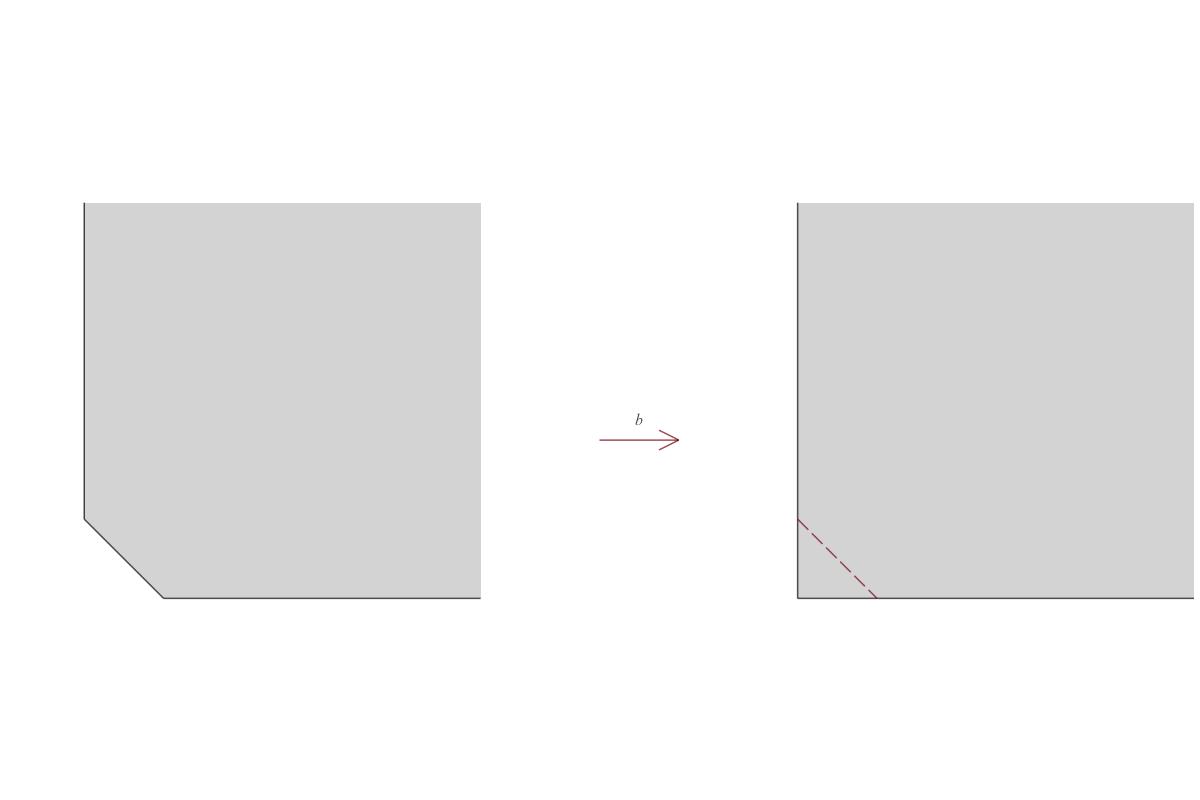
Figure 1.1. The polytopes of ${\widehat{\mathbb{C}}^{2}_{0}}$ and ${\mathbb{C}}^{2}$.

We thus get the following

Theorem 1.4.

Let $M_{\Delta}^{{\mathbb{C}}}$ be the compact complex manifold associated to a Delzant polytope $\Delta\subset{\mathbb{R}}^{m}$ with respect to the standard lattice ${\mathbb{Z}}^{m}\subset({\mathbb{R}}^{m})^{*}$. Let $w_{1},w_{2},\ldots,w_{m}$ be primitive inward-pointing edge vectors at a vertex $v$ of $\Delta$ and $\hat{\Delta}_{\varepsilon}$ the polytope obtained from $\Delta$ by replacing $v$ with the $m$-vertices $v+\varepsilon w_{i}$, $i=1,\ldots,m$ for some $\varepsilon>0$. Then, $\hat{\Delta}_{\varepsilon}$ is Delzant polytope too, and the corresponding complex manifold $M_{\hat{\Delta}_{\varepsilon}}^{{\mathbb{C}}}$ is obtained from $M_{\Delta}^{{\mathbb{C}}}$ by blowing up a fixed point for the torus action.

Exercise 1.6.

Identify the complex manifolds and the equivariant blowdown maps corresponding to the Delzant polytopes of Figure 2.

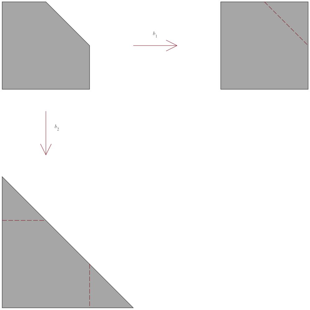
Figure 1.2.

.

1.7. Polarized projective toric varieties

There is a third facet of the story, which relates the smooth compact toric symplectic manifolds to the theory of polarized projective varieties. Recall that a smooth polarized projective complex variety is a compact complex manifold $M$ of complex dimension $m$, endowed with a very ample holomorphic line bundle $L\to M$, i.e. a holomorphic line bundle such that the Kodaira map [23]

$$\kappa:M\longrightarrow\mathrm{P}(W^{*}),$$

where $W=H^{0}(M,L)$ is the $(N+1)$-dimensional complex vector space of holomorphic sections of $L$, is a holomorphic embedding and $L=\kappa^{*}{\mathcal{O}}(1)_{W^{*}}$. In this case, one can identify $(M,L)$ with its embedded image $\tilde{M}=\kappa(M)\subset\mathrm{P}(W^{*})\cong{\mathbb{C}}P^{N},$ by considering the polarization of $\tilde{M}$ defined by the the restriction of the anti-tautological line bundle ${\mathcal{O}}(1)$ of ${\mathbb{C}}P^{N}$. In this setting, we have

Definition 1.9.

A toric polarized projective variety $\tilde{M}\subset{\mathbb{C}}P^{N}$ is an $m$-dimensional complex submanifold of ${\mathbb{C}}P^{N}$ which is the (Zariski) closure in ${\mathbb{C}}P^{N}$ of a principal orbit for the action of a complex $m$-dimensional complex torus ${\mathbb{T}}^{{\mathbb{C}}}\subset{\bf SL}(N+1,{\mathbb{C}})$ on ${\mathbb{C}}P^{N}$.

Denote by ${\mathbb{T}}$ the real $m$-dimensional torus corresponding to ${\mathbb{T}}^{{\mathbb{C}}}$, and let ${\mathbb{T}}^{N}\subset{\bf SL}(N+1,{\mathbb{C}})$ be a maximal real torus containing ${\mathbb{T}}$. As discussed in Section 1.3, ${\mathbb{C}}P^{N}$ admits a ${\mathbb{T}}^{N}$-invariant Fubini–Study Kähler metric $\omega^{FS}$ and it is not difficult to show that $2\omega^{FS}$ is the curvature of a ${\mathbb{T}}^{N}$-invariant hermitian metric on ${\mathcal{O}}(1)$. Restricting to $\tilde{M}$, we obtain a ${\mathbb{T}}$-invariant symplectic form $\omega$ on $\tilde{M}$, belonging to the deRham class $2\pi c_{1}(L)$. The ${\mathbb{T}}$-action is hamiltonian with respect to this symplectic structure, since ${\mathbb{T}}\subset{\mathbb{T}}^{N}\subset{\bf SL}(N+1,{\mathbb{C}})$ and the action of ${\mathbb{T}}^{N}$ is hamiltonian with respect to $2\omega^{FS}$. We thus have

Proposition 1.3.

Any smooth polarized toric complex variety is a symplectic toric manifold.

From the considerations in Section 1.5, we get a correspondence between smooth toric projective varieties and complex toric varieties defined via the Delzant construction. It is however not entirely clear how this correspondence translates in terms of Delzant polytopes or, in other words, how to construct a polarized toric variety from a given Delzant polytope. To explain this, we give the following

Definition 1.10 (Lattice polytopes).

Suppose $(\Delta,{\bf L},\Lambda)$ is a Delzant polytope as in Definition 1.5. We say that $(\Delta,{\bf L},\Lambda)$ is a lattice Delzant polytope if, moreover, all vertices of $\Delta$ belong to the dual lattice $\Lambda^{*}\subset V$.

For any lattice Delzant polytope, we can take a basis $\{e_{1},\ldots,e_{m}\}$ of $\Lambda$ and consider $\Delta\subset{\mathbb{R}}^{m}$ with the standard lattice $\Lambda^{*}={\mathbb{Z}}^{m}\subset{\mathbb{R}}^{m}$; the fact that $(\Delta,{\bf L},\Lambda)$ is a lattice Delzant polytope translates to the fact that the vertices of $\Delta$ are in ${\mathbb{Z}}^{m}$ (see Exercise 1.2). We denote by

$$A(\Delta):=\{\lambda^{(j)}=(\lambda_{1}^{(j)},\ldots,\lambda_{m}^{(j)}),j=0,\ldots,N\}$$

all the lattice points in $\Delta$. We then consider the $({\mathbb{C}}^{*})^{m}$-action on ${\mathbb{C}}P^{N}$, given in homogeneous coordinates by

$$(z_{1},\ldots,z_{m})\cdot[w_{0},\ldots,w_{N}]:=[(z_{1}^{\lambda_{1}^{(0)}}\cdots z_{m}^{\lambda^{(0)}_{m}})w_{0},\ldots,(z_{1}^{\lambda_{1}^{(N)}}\cdots z_{m}^{\lambda_{m}^{(N)}})w_{N}].$$

We associate to such a data the toric polarized variety $M_{A(\Delta)}\subset{\mathbb{C}}P^{N}$ which is the Zariski closure in ${\mathbb{C}}P^{N}$ of the $({\mathbb{C}}^{*})^{m}$-orbit of the point $[1,\ldots,1]\in{\mathbb{C}}P^{N}$ for this action. The basic fact is the following

Theorem 1.5 (Section 6.6 in [9]).

For any lattice Delzant polytope $\Delta$, $M_{A(\Delta)}\subset{\mathbb{C}}P^{N}$ is a smooth polarized toric projective variety whose Delzant polytope with respect to a ${\mathbb{T}}^{m}$-invariant Fubini–Study symplectic form in $2\pi c_{1}({\mathcal{O}}(1))$ is $\Delta\subset{\mathbb{R}}^{m}$ with lattice $\Lambda^{*}={\mathbb{Z}}^{m}$. In particular, $M_{A(\Delta)}$ is biholomorphic to the complex manifold $M^{{\mathbb{C}}}_{\Delta}$ defined in Section 1.5.

Example 1.8.

Let $\Delta\subset{\mathbb{R}}^{m}$ be the lattice Delzant simplex, defined by

$$\Delta=\{L_{0}=(1-\sum_{j=1^{n}}x_{j})\geq 0,L_{j}(x)=x_{j}\geq 0,j=1,\ldots m\}$$

and the standard lattice ${\mathbb{Z}}^{m}\subset({\mathbb{R}}^{m})$. $\Delta$. The set of lattice points of $\Delta$ is

$$A(\Delta)=\{\lambda^{(0)}=(0,\ldots,0),\lambda^{(j)}=e_{j},j=1,\ldots,m\},$$

where $e_{j}$ is the standard basis of ${\mathbb{R}}^{m}$. The Delzant construction identifies the corresponding symplectic toric manifold with $({\mathbb{C}}P^{m},2\omega^{FS})$, whereas Theorem 1.5 realizes $M_{A(\Delta)}$ as the closure in ${\mathbb{C}}P^{m}$ of a principal $({\mathbb{C}}^{*})^{m}$-orbit for the action

$$(z_{1},\ldots,z_{m})\cdot[w_{0},\ldots,w_{m+1}]=[w_{0},z_{1}w_{1},\ldots,z_{m}w_{m}],$$

which clearly is ${\mathbb{C}}P^{m}$. The induced symplectic structure on this polarized variety is again $2\omega^{FS}$.

Exercise 1.7.

Let $M_{A(\Delta)}\subset{\mathbb{C}}P^{N}$ be a toric polarized projective variety corresponding to a lattice Delzant polytope $\Delta\subset{\mathbb{R}}^{m}$ with respect to the lattice ${\mathbb{Z}}^{m}\subset{\mathbb{R}}^{m}$. Using that the sections of ${\mathcal{O}}(1)$ are identified with linear functions in homogeneous coordinates $[w_{0},\ldots,w_{N}]$ on ${\mathbb{C}}P^{N}$, show that the $({\mathbb{C}}^{*})^{m}$-action on $M_{A(\Delta)}$ defines a $({\mathbb{C}}^{*})^{m}$-action on the vector space $H^{0}(M_{A(\Delta)},L)$ of holomorphic sections of $L$. Furthermore, show that here is a basis $\{s_{0},\ldots,s_{N}\}$ of $H^{0}(M_{A(\Delta)},L)$, parametrized by the lattice points $\{\lambda^{(0)},\ldots,\lambda^{(N)}\}$ in $A(\Delta)$, such that $({\mathbb{C}}^{*})^{m}$ acts on $s_{j}$ by

$$(z_{1},\ldots,z_{m})\cdot s_{j}=(z_{1}^{\lambda_{1}^{(j)}}\cdots z_{m}^{\lambda_{m}^{(j)}})s_{j}.$$

1.8. Toric orbifolds

We briefly discuss here what happens with the Delzant construction reviewed in Section 1.4 when one starts with a rational Delzant triple $(\Delta,{\bf L},\Lambda)$, i.e satisfying the weaker conditions (i)-(ii)-(iii)’ of Definition 1.5. There are two points in the construction which deserve a special attention.

The first point is Claim 1. Consider for example the labelled Delzant simplex $(\Delta_{m},{\bf L})$ with ${\bf L}=\{L_{j}(x)=x_{j},j=1,\ldots m,L_{m+1}(x)=-\sum_{j=1}^{m}x_{j}+\frac{1}{2}\}$, corresponding to $({\mathbb{C}}P^{m},\omega^{FS}),$ and change the standard lattice $\Lambda={\mathbb{Z}}_{m}\subset({\mathbb{R}}^{m})^{*}$ with the lattice $\Lambda^{\prime}=\frac{1}{2}\Lambda$. The condition (iii)’ then holds for the triple $(\Delta_{m},{\bf L},\Lambda^{\prime})$. However, in this case,

$$N^{\prime}={\rm Ker}(\tau)=\mathbb{S}^{1}\times{\mathbb{Z}}_{2}^{m},$$

where ${\mathbb{Z}}_{2}^{m}:=(\pm 1,\pm 1,\ldots,\pm 1)\subset{\mathbb{T}}^{m+1}$. In particular, $N^{\prime}$ is no longer connected. Following the construction further, the quotient space will be

$$M^{\prime}={\mathbb{S}}^{2m+1}/N^{\prime}={{\mathbb{C}}P^{m}}/{{\mathbb{Z}}}^{m}_{2}.$$

Such a space is an example of an orbifold.

Definition 1.11.

An orbifold chart on a topological space $M$ is a triple $(\hat{U},\Gamma,\varphi)$ where:

1. $\hat{U}\subset{\mathbb{R}}^{n}$ is an open subset;

2. $\Gamma\subset{\bf GL}(n)$ is a finite subgroup acting on $\hat{U}$

3. $\varphi:\hat{U}/\Gamma\to M$ is a homeomorphism between $\hat{U}/\Gamma$ and an open subset $V\subset M$.

We denote by $\hat{\varphi}:\hat{U}\to M$ the induced $\Gamma$-invariant map.

An embedding between two orbifold charts $(\hat{U}_{1},\Gamma_{1},\hat{\varphi}_{1})$ and $(\hat{U}_{2},\Gamma_{2},\hat{\varphi}_{2})$ is a smooth embedding $\lambda:\hat{U}_{1}\to\hat{U}_{2}$ such that $\hat{\varphi}_{1}=\hat{\varphi}_{2}\circ\lambda$.

Two orbifold charts $(\hat{U}_{1},\Gamma_{1},\hat{\varphi}_{1})$ and $(\hat{U}_{2},\Gamma_{2},\hat{\varphi}_{2})$ are compatible if there exists an open subset $V\subset V_{1}\cap V_{2}$ (where we have set $V_{i}=\hat{\varphi}_{i}(\hat{U}_{i})$) and an orbifold chart $(\hat{U},\Gamma,\hat{\varphi})$ with $\hat{\varphi}(\hat{U})=V$, and two embeddings $\lambda_{i}:\hat{U}\to\hat{U}_{i},i=1,2$.

An orbifold $M$ of (real) dimension $n$ is a Hausdorff paracompact topological space, endowed with an open covering of compatible orbifold charts $\{(\hat{U}_{i},\Gamma_{i},\hat{\varphi}_{i})\}_{i\in I}$. A smooth function $f:M\to{\mathbb{R}}$ on an orbifold $M$ is defined by the property that on each orbifold chart $(\hat{U},\Gamma,\hat{\varphi})$, it pulls-back by $\hat{\varphi}$ to a $\Gamma$-invariant smooth function on $\hat{U}$. One can define smooth tensors on $M$ is a similar way.

The above phenomenon can be remedy by taking $\Lambda_{\rm min}={\rm span}_{{\mathbb{Z}}}\{u_{1},\ldots u_{d}\},$ which is the minimal (under the inclusion) lattice for which the condition (iii)’ is satisfied for the given labelling ${\bf L}$. The subgroup $N_{\rm min}$ will be then a torus and for any other choice of lattice $\Lambda$, the produced quotient space $S/N$ will be a quotient of $S/N_{\rm min}$ by the finite abelian group $\Lambda/\Lambda_{\rm min}$. Geometrically, this is translated to taking orbifold coverings, $S/N_{\rm min}$ being the simply connected orbifold covering all other quotients, see Thurston [50].

The second point is Claim 4. When we assume (iii)’ instead of (iii), the stabilizers for the ${\mathbb{T}}^{d}$-action on $S$ will be finite abelian groups, and in general so be the stabilizers of the action of $N$. However, once again the quotient space $S/N$ will be an orbifold in the sense of the above definition.

To summarize, we observed that

Proposition 1.4.

Suppose $(\Delta,{\bf L},\Lambda)$ is a rational Delzant triple, i.e. satisfies the conditions (i)-(ii)-(iii)’ of Definition 1.5. Then the Delzant construction associates to $(\Delta,{\bf L},\Lambda)$ a compact symplectic orbifold $(M,\omega)$ endowed with a Hamiltonian action of the torus ${\mathbb{T}}=V/2\pi\Lambda$ and momentum image $\Delta$.

The converse is also true, due to the following extension of Delzant’s correspondence to toric orbifolds

Theorem 1.6 (Lerman–Tolman [37]).

Compact symplectic orbifolds modulo equivalence are in bijective correspondence with rational Delzant triples modulo the action of the affine group.

We give below one specific example

Example 1.9 (The weighted projective spaces).

Similarly to the way we introduced the complex projective space, we can consider for any $(m+1)$-tuple of positive integers ${\bf a}=(a_{0},\ldots,a_{m})$ with ${g.c.d}(a_{0},\ldots,a_{m})=1$ the quotient space

$${\mathbb{C}}P^{m}_{\bf a}={\mathbb{C}}^{m+1}\setminus\{0\}/{\mathbb{C}}^{*}_{\bf a},$$

where ${\mathbb{C}}^{*}_{\bf a}$ denotes the ${\mathbb{C}}^{*}$ action $\rho_{\bf a}$ on ${\mathbb{C}}^{m+1}=(z_{0},\ldots,z_{m})$ by

$$\rho_{\bf a}(\lambda)(z):=(\lambda^{a_{0}}z_{0},\ldots,\lambda^{a_{m}}z_{m}).$$

Lemma 1.4.

${\mathbb{C}}P^{m}_{\bf a}$ is an orbifold, which is diffeomorphic (as an orbifold) to the quotient space

$${\mathbb{S}}^{2m+1}/{\mathbb{S}}^{1}_{\bf a}$$

where ${\mathbb{S}}^{1}_{\bf a}$ stands for the circle action $\rho_{\bf a}$ on ${\mathbb{S}}^{2m+1},$ given by

$$\rho_{\bf a}(e^{\sqrt{-1}t})(z)=(e^{\sqrt{-1}a_{0}t},\ldots,e^{\sqrt{-1}a_{m}t}).$$

The proof of this result is left as an exercise. We can now easily modify the construction of the toric structure on ${\mathbb{C}}P^{m}$ and get the following

Lemma 1.5.

The orbifold ${\mathbb{C}}P_{\bf a}^{m}$ admits a toric Kähler structure $(g,\omega,J)$ obtained by the Delzant construction starting with the rational Delzant triple $(\Delta_{m},{\bf L}_{\bf a},\Lambda_{\bf a})$ where $\Delta_{m}\subset{\mathbb{R}}^{m}$ is the standard simplex labelled as

$$\begin{split}\Delta_{m}:=&\Big{\{}(x_{1},\ldots,x_{m}):L_{j}(x)=\Big{(}\frac{a_{0}\cdots a_{m}}{a_{j}}\Big{)}x_{j}\geq 0,j=1,\ldots,m,\\ &\ \ \ \ \ L_{m+1}(x)=\Big{(}\frac{a_{0}\cdots a_{m}}{a_{0}}\Big{)}\Big{(}\frac{1}{2}-\sum_{j=1}^{m}x_{j}\Big{)}\geq 0\Big{\}},\end{split}$$

and the lattice $\Lambda_{\bf a}$ is defined by

$$\Lambda_{\bf a}:={\rm span}_{{\mathbb{Z}}}\Big{\{}\Big{(}\frac{a_{0}\cdots a_{m}}{a_{j}}\Big{)}e_{j}^{*},\ j=1,\ldots,m,\ \Big{(}\frac{a_{0}\cdots a_{m}}{a_{0}}\Big{)}(e_{1}^{*}+\cdots+e_{m}^{*})\Big{\}}$$

where $\{e_{j}^{*}\}_{j=1}^{m}$ stands for the standard basis of $({\mathbb{R}}^{m})^{*}$.

Chapter 2 Abreu–Guillemin Theory

2.1. The orbit space of a toric manifold

Let $(M,\omega,{\mathbb{T}})$ be a toric symplectic manifold and $\mu:M\to\Delta$ the corresponding Delzant polytope. We denote by

$$M_{\rm red}:=M/{\mathbb{T}}$$

the space of orbits for the ${\mathbb{T}}$-action on $M$, which is a compact Hausdorff space with respect to the quotient topology, see e.g. [5]. The momentum map $\mu$ being ${\mathbb{T}}$-invariant descends to a continuous map $\check{\mu}:M_{\rm red}\to\Delta$. Some important ingredients in Delzant’s theorem are the following

Fact 1. $\check{\mu}$ is a bijection.

Fact 2. Delzant’s proof [15] shows that the pre-image $p=\mu^{-1}(x)$ of a point $x\in\Delta$ situated on an open face $F^{0}\subset\Delta$ of co-dimension $\ell$ has a stabilizer ${\mathbb{T}}_{p}$ which is a torus of dimension $\ell$. In particular, the pre-image of a point $x\in\Delta^{0}$ is a principal orbit isomorphic to ${\mathbb{T}}$. We shall denote $M^{0}:=\mu^{-1}(\Delta^{0})$ the dense open subset of $M$ consisting of points having principal orbits. As ${\mathbb{T}}$ acts freely on $M^{0}$, $\mu:M^{0}\to\Delta^{0}$ is a principal ${\mathbb{T}}$-bundle over $\Delta^{0}$.

Another fact coming from [15] is

Fact 3. $M_{\rm red}$ and $\Delta$ both admit “differentiable structure” of manifolds with corners induced from the smooth structure of $M$, and $\check{\mu}$ is a diffeomorphism in this category, ([32], Proposition C7).

Exercise 2.1.

Check Facts 1–3 for the symplectic manifold $(M,\omega)$ associated to a Delzant polytope $(\Delta,{\bf L},\Lambda)$ via the construction in Section 1.4.

The differentiable structure on $\Delta\subset\mathfrak{t}^{*}$ is the one naturally induced by restricting to $\Delta$ the smooth functions on $\mathfrak{t}^{*}$. To see how it is related to the smooth structure on $M$, we notice the following

Lemma 2.1.

(Schwarz [48]) A ${\mathbb{T}}$-invariant function $f(p)$ on $M$ is smooth iff

$$f(p)=\varphi(\mu(p))$$

for some smooth function $\varphi(x)$ on $\mathfrak{t}^{*}$.

In the case when $(M,\omega,{\mathbb{T}})=({\mathbb{R}}^{2},\omega_{0},{\mathbb{S}}^{1})$, this is a well-know result by Whitney; in general, Lemma 2.1 can be easily derived from ([15], Lemme 5). Because of this basic fact, we shall often write $f(x)$ for the composition $f(p)=\varphi(\mu(p))$.

2.2. Toric Kähler metrics: local theory

To simplify the presentation, we fix a basis $\{e_{1},\ldots,e_{m}\}$ of ${\mathfrak{t}}$ and denote by $K_{j}=X_{e_{j}}$ the induced fundamental vector fields; we shall also identify ${\mathfrak{t}}^{*}\cong({\mathbb{R}}^{m})^{*}$ by using the dual basis $\{e_{1}^{*},\ldots,e_{m}^{*}\}$ and write $x=(x_{1},\ldots,x_{m})$ for the elements of ${\mathfrak{t}}^{*}$. As explained in the previous section, on $M^{0}$, $K_{1},\ldots,K_{m}$ are functionally independent, i.e. for each point $p\in M^{0}$, $(K_{1}\wedge\cdots\wedge K_{m})(p)\neq 0$. We shall also identify the coordinate function $x_{i}=\langle x,e_{i}\rangle$ with the momentum function $\langle\mu,e_{i}\rangle$ on $M$, i.e. we write

(2.1) $$\imath_{K_{i}}\omega=-dx_{i}.$$

Let $(g,J)$ be a ${\mathbb{T}}$-invariant $\omega$-compatible Kähler structure on $M$. Letting

$$H_{ij}=g(K_{i},K_{j})$$

we get a ${\mathbb{T}}$-invariant smooth function on $M$, which will tacitly identify with a smooth function $H_{ij}(x)$ on $\Delta$, see Fact 2 above. We denote by ${\bf H}_{x}=(H_{ij}(x))$ the corresponding symmetric matrix with smooth entries over $\Delta$. In a more intrinsic language, we regard ${\bf H}$ as a smooth function over $\Delta$ with values in $S^{2}{\mathfrak{t}}^{*}$ by letting

$${\bf H}_{x}(\xi_{1},\xi_{2}):=g_{p}(X_{\xi_{1}},X_{\xi_{2}})$$

for any $\xi_{1},\xi_{2}\in{\mathfrak{t}}$ and any $p\in\mu^{-1}(x)$.

On $\Delta^{0}$, ${\bf H}$ is positive definite and we denote by ${\bf G}:={\bf H}^{-1}$ the inverse matrix; equivalently, ${\bf G}$ is a smooth $S^{2}{\mathfrak{t}}$-valued function on $\Delta^{0}$.

Notice that, by (2.1),

(2.2) $$dx_{i}(JK_{j})=-\omega(K_{i},JK_{j})=--g(JK_{i},JK_{j})=-g(K_{i},K_{j})=-H_{ij}(x).$$

We now consider the vector fields $\{K_{1},\ldots,K_{m},JK_{1},\ldots,JK_{m}\}$. They form a basis of $T_{p}M$ at each $p\in M^{0}$ (because $\{K_{1},\ldots,K_{m}\}$ span an $m$-dimensional space and $\{JK_{1},\ldots,JK_{m}\}$ span its $g$-orthogonal complement) and satisfy

(2.3) $$[K_{i},K_{j}]=[K_{i},JK_{j}]=[JK_{i},JK_{j}]=0,$$

where for the second identity we used that ${\mathbb{T}}$ preserves $J$, whereas for the third identity we used the integrability of $J$, see (1.8). We now denote by

$$\{\theta_{1},\ldots,\theta_{m},J\theta_{1},\ldots,J\theta_{m}\}$$

the dual basis of $T^{*}M^{0},$ corresponding to

$$\{K_{1},\ldots,K_{m},JK_{1},\ldots,JK_{m}\},$$

where for a $1$-form $\theta$ we set $J\theta(X)=-\theta(JX)$, for any vector field $X$. The commuting relation (2.3) is equivalent to

(2.4) $$d\theta_{i}=0=d(J\theta_{i}),\ \ i=1,\ldots m.$$

As the $1$-forms $J\theta_{i}$ satisfy

$$\imath_{K_{j}}J\theta_{i}=0,\ \ \mathcal{L}_{K_{j}}J\theta_{i}=0,$$

in terms of the ${\mathbb{T}}$-bundle structure $\mu:M^{0}\to\Delta 0$, each $J\theta_{i}$ is basic, i.e. $J\theta_{i}=\mu^{*}(\alpha_{i})$ of a closed $1$-form $\alpha_{i}$ on $\Delta^{0}$. As $\Delta^{0}$ is contractible, we can write

(2.5) $$J\theta_{i}=-dy_{i}$$

for some smooth function $y_{i}(x),$ defined on $\Delta^{0}$ up to an additive constant (as usual, we omit the pull-back by $\mu$ in the notation). Furthermore, by (2.2), we find

(2.6) $$\begin{split}-J\theta_{i}&=dy_{i}=\sum_{j=1}^{m}G_{ij}(x)dx_{j},\\ Jdx_{i}&=\sum_{j=1}^{m}H_{ij}(x)\theta_{j}.\end{split}$$

The $1$-forms $\{\theta_{1},\ldots,\theta_{m}\}$ define a $1$-form ${\boldsymbol{\theta}}$ with values ${\mathfrak{t}}={\rm Lie}({\mathbb{T}})$, by letting

(2.7) $${\boldsymbol{\theta}}=\sum_{i=1}^{m}\theta_{i}\otimes e_{i},$$

whose curvature is identically zero. The symplectic $2$-form $\omega$ then becomes

(2.8) $$\omega:=\langle d\mu\wedge{\boldsymbol{\theta}}\rangle=\sum_{i=1}^{m}dx_{i}\wedge\theta_{i},$$

whereas the Kähler metric is

(2.9) $$\begin{split}g&=\sum_{i,j=1}^{m}g(K_{i},K_{j})\Big{(}\theta_{i}\otimes\theta_{j}+J\theta_{i}\otimes J\theta_{j}\Big{)}\\ &=\sum_{i,j=1}^{m}H_{ij}\Big{(}\theta_{i}\otimes\theta_{j}+dy_{i}\otimes dy_{j}\Big{)}\\ &=\sum_{i,j=1}^{m}\Big{(}G_{ij}dx_{i}\otimes dx_{j}+H_{ij}\theta_{i}\otimes\theta_{j}\Big{)}\\ &=\langle d\mu,{\bf G},d\mu\rangle+\langle{\boldsymbol{\theta}},{\bf H},{\boldsymbol{\theta}}\rangle.\end{split}$$

Lemma 2.2 (Guillemin [25]).

Let $(M,\omega,{\mathbb{T}})$ be a symplectic toric manifold with Delzant polytope $\Delta$ and $(g,J)$ an $\omega$-compatible ${\mathbb{T}}$-invariant Kähler structure. Then, on $M^{0}$, $(g,\omega)$ can be written in the form (2.8)–(2.9), where $G_{ij}=\frac{\partial^{2}u}{\partial x_{i}\partial x_{j}}$ for a smooth, strictly convex function $u(x)$ on $\Delta^{0}$, called symplectic potential of $g$. Conversely, for any strictly-convex smooth function $u$ on $\Delta^{0}$, the riemannian metric on $M^{0}$ defined by (2.9) with ${\bf G}={\rm Hess}(u),\ {\bf H}={\bf G}^{-1}$ and the flat connection $1$-form ${\boldsymbol{\theta}}$ defines an $\omega$-compatible, ${\mathbb{T}}$-invariant Kähler structure on $M^{0}$.

Proof.

We shall denote with subscript $f_{,k}$ the partial derivative $\frac{\partial f}{\partial x_{k}}$ of a smooth function $f$ on $\Delta$. Letting

$$\beta:=\sum_{i=1}^{m}y_{i}dx_{i},$$

we have by (2.6)

$$d\beta=\sum_{i=1}^{m}dy_{i}\wedge dx_{i}=\sum_{i,j=1}^{m}G_{ij}dx_{i}\wedge dx_{j}=0.$$

By the Poincaré Lemma on $\Delta^{0}$, $\beta=du$ for some smooth function $u$ on $\Delta^{0}$, i.e. $y_{i}=u_{,i}$. It follows that

(2.10) $$G_{ij}=y_{i,j}=u_{,ij}=({\rm Hess}(u))_{ij}$$

Conversely, for the metric (2.9), we let $G_{ij}=g(K_{i},K_{j})$ and suppose that (2.10) holds true. It follows that the $1$-forms

$$-J\theta_{i}=\sum_{j=1}^{m}G_{ij}dx_{j}=\sum_{j=1}^{m}u_{,ij}dx_{j}$$

are closed. As $\theta_{i}$ are closed too (by the assumption that ${\boldsymbol{\theta}}$ is flat), we get a basis of $\Lambda^{1,0}(M^{0},J)$ of closed $(1,0)$-forms $-J\theta_{i}+\sqrt{-1}\theta_{i}$, so writing locally $-J\theta_{i}+\sqrt{-1}\theta_{i}=dy_{i}+\sqrt{-1}dt_{i}$ we get holomorphic coordinates $y_{i}+\sqrt{-1}t_{i}$ for $J$, i.e. $J$ is integrable. ∎

We have seen in Chapter 1 that the action of ${\mathbb{T}}\cong(\mathbb{S}^{1})^{m}$ on $(M,J)$ extends to an (effective) holomorphic action of the complex torus ${\mathbb{T}}^{{\mathbb{C}}}\cong({\mathbb{C}}^{*})^{m}$. Fixing a point $p_{0}\in M^{0}$, we can identify $M^{0}$ with the orbit ${\mathbb{T}}^{{\mathbb{C}}}(p_{0})\cong({\mathbb{C}}^{*})^{m}$. Using the polar coordinates $(r_{i},t^{0}_{i})$ on each ${\mathbb{C}}^{*}$, this identification gives rise the so-called angular coordinates

$$\boldsymbol{t}=(t^{0}_{1},\ldots,t^{0}_{m}):M^{0}\to\mathfrak{t}/2\pi\Lambda.$$

If another reference point is chosen, $\boldsymbol{t}$ varies by an additive constant in $\mathfrak{t}$. Writing $\boldsymbol{\theta}=d\boldsymbol{t}$, we have

Definition 2.1.

For a fixed $\omega$-compatible, ${\mathbb{T}}$-invariant complex structure $J$ on $(M,\omega,{\mathbb{T}})$ (corresponding to a symplectic potential $u(x)$ on $\Delta^{0}$), and a base point $p_{0}\in M^{0}$ (giving rise to angular coordinates ${\bf t}=\sum_{i=1}^{m}t_{i}e_{i}$ with respect to a basis $e=\{e_{1},\ldots,e_{m}\}$ of ${\mathfrak{t}}$), the functions $\{x_{1},\ldots,x_{m};t_{1},\ldots,t_{m}\}$ on $\Delta^{0}\times{\mathbb{T}}$ are called momentum-angle coordinates associated to $(g,J)$.

2.3. The scalar curvature

Recall that if $(M^{2m},J,g,\omega)$ is a Kähler manifold, the riemannian metric $g$ induces a hermitian metric (still denoted by $g$) on the anti-canonical complex line bundle $K^{-1}(M)=\wedge^{m}(T^{1,0}M)$, where $TM\otimes{\mathbb{C}}=T^{1,0}M\oplus T^{0,1}M$ is the type decomposition of the complexified tangent bundle of $M$ into $\sqrt{-1}$ and $-\sqrt{-1}$ eigen-spaces of $J$. Furthermore, $K^{-1}(M)$ has a canonical holomorphic structure, induced by the holomorphic structure of $T^{1,0}M$ (for which the holomorphic vector fields are the holomorphic sections). The Ricci-form $\rho^{g}$ of $g$ is defined in terms of the curvature of the Chern connection $\nabla^{g}$ of $(K^{-1}(M),g)$, by

$$R_{X,Y}^{\nabla^{g}}=\sqrt{-1}\rho_{g}(X,Y).$$

In the Kähler case, $\nabla^{g}$ coincides with the induced connection on $K^{-1}(M)$ by the Levi–Civita connection of $g$, and the $2$-form $\rho_{g}$ is essentially the Ricci tensor ${\rm Ric}_{g}$ of $g$, i.e. we have

$$\rho_{g}(X,Y)={\rm Ric}_{g}(JX,Y).$$

It thus follows that the scalar curvature $s_{g}:={\rm tr}_{g}({\rm Ric}_{g})$ of $g$ is equivalently given by

(2.11) $$s_{g}={\rm tr}_{\omega}(\rho_{g}):=2m\Big{(}(\rho_{g}\wedge\omega^{m-1})/\omega^{m}\Big{)}.$$

We now consider a ${\mathbb{T}}$-invariant, $\omega$-compatible Käher metric on a symplectic toric manifold $(M,\omega,{\mathbb{T}})$, written on $M^{0}$ in the form (2.9) where ${\bf G}={\rm Hess}(u)$ for a symplectic potential $u\in S(\Delta,{\bf L})$.

Lemma 2.3 (Abreu [1]).

The Ricci form of $(g,J)$ is given by

$$\rho_{g}=-\frac{1}{2}\sum_{i,j,k=1}^{m}H_{ij,ik}dx_{k}\wedge\theta_{j}$$

whereas the scalar curvature is

$$s_{g}=-\sum_{i,j=1}^{m}H_{ij,ij},$$

where we recall that for $u\in S(\Delta,{\bf L})$, $H_{ij}=({\rm Hess}(u))^{-1}_{ij}=u^{,ij}$.

Proof.

As the fundamental vector fields $K_{i}$ preserve $J$,

$$\sigma:=(K_{1}-\sqrt{-1}JK_{1})\wedge\cdots\wedge(K_{m}-\sqrt{-1}JK_{m})$$

is a holomorphic section on $K^{-1}(M)$ which does not vanish on $M^{0}$. It is a well-known fact (see e.g. [56]) that the (Chern) Ricci form is then given on $M^{0}$ by

$$\rho_{g}=-\frac{1}{2}dd^{c}\log|\sigma|_{g}^{2}.$$

In our case, $|\sigma|_{g}^{2}=2^{m}{\rm det}(g(K_{i},K_{j}))={\rm det}\ {\bf H}$, so we obtain

$$\begin{split}d^{c}\log\det{\bf H}&={\rm tr}\Big{(}{\bf H}^{-1}d^{c}{\bf H}\Big{)}=\sum_{i,j,k}G_{ij}H_{ij,k}Jdx_{k}\\ &=\sum_{i,j,k,\ell}G_{ij}H_{ij,k}H_{k\ell}\theta_{\ell}\\ &=-\sum_{i,j,k,\ell}G_{ij,k}H_{ij}H_{k\ell}\theta_{\ell}\\ &=-\sum_{i,j,k,\ell}G_{ik,j}H_{ij}H_{k\ell}\theta_{\ell}\\ &=\sum_{i,j,k,\ell}G_{ik}H_{ij}H_{k\ell,j}\theta_{\ell}\\ &=\sum_{j,\ell}H_{j\ell,j}\theta_{\ell}.\end{split}$$

We then compute

(2.12) $$\begin{split}\rho_{g}&=-\frac{1}{2}dd^{c}\log\det{\bf H}\\ &=-\frac{1}{2}\sum_{i,j,k}H_{ij,ik}dx_{k}\wedge\theta_{j}.\end{split}$$

The formula for $s_{g}$ follows from (2.11), by using that $\omega=\sum_{i}dx_{i}\wedge\theta_{i}$ and (2.12). ∎

2.4. Symplectic versus complex: the Legendre transform

We now turn our attention to the function $y_{j}=u_{,j}$ on $M^{0}$ introduced in (2.6). For a choice of angular coordinates $\theta_{j}=dt_{j}$ we have $-J\theta_{j}+\sqrt{-1}\theta_{j}=dy_{j}+\sqrt{-1}dt_{j}$ and $y_{j}+\sqrt{-1}t_{j}$ define $J$-holomorphic coordinates on $M^{0}$; exponentiating, we obtain another set of holomorphic coordinates $z_{j}:=e^{y_{j}}e^{\sqrt{-1}t_{j}}$ on $M^{0}$.

Now, choosing $\{e_{1},\ldots,e_{m}\}$ to be a basis of $\Lambda$, and considering the action of the flows of $\{K_{1},\ldots,K_{m};JK_{1},\ldots,JK_{m}\}$ around the reference point $p_{u}\in M^{0}$ corresponding to the unique minima $x_{u}\in\Delta^{0}$ of $u$ under the momentum map and $t_{j}(p_{0})=0$, we see that $(z_{1},\ldots,z_{m})$ provide an ${\mathbb{T}}^{{\mathbb{C}}}$ equivariant identification

(2.13) $$\Phi_{p_{u},u,e}:({\mathbb{C}}^{*})^{m}\cdot p_{u}\cong(M^{0},J),$$

A subtle point in the construction is that $\Phi_{p_{u},u,e}$ depends upon the choice of $u$ and the basis $e=\{e_{1},\ldots,e_{m}\}$ of $\mathfrak{t}$.

Definition 2.2 (Legendre transform).

Let $u$ be a strictly convex smooth function on $\Delta^{0}$. Letting $y_{j}(x):=u_{,j}(x)$ and

$${y}(x):=\sum_{i=1}^{m}y_{i}(x)e_{i}=(du)_{x}\in(T_{x}\Delta^{0})^{*}\cong({\mathfrak{t}}^{*})^{*}={\mathfrak{t}}$$

be the map from $\Delta^{0}$ to ${\mathfrak{t}}$, we define the Legendre transform of $u(x)$ to be the function $\phi(y)=\phi(y_{1},\ldots,y_{m})$ satisfying

(2.14) $$\phi(y(x))+u(x)=\langle y(x),x\rangle,$$

where ${x}=\sum_{i=1}^{m}x_{i}e_{i}^{*}$ is seen as a smooth function from $\Delta^{0}$ to ${\mathfrak{t}}^{*}$.

Lemma 2.4 (Guillemin [25]).

Let $(g,J)$ be an $\omega$-compatible, ${\mathbb{T}}$-invariant Kähler structure on $(M,\omega,{\mathbb{T}})$ with symplectic potential $u(x)$ defined on $\Delta^{0}$. Then, the Legendre transform $\phi(y)$ of $u(x)$ is a Kähler potential of the symplectic form $\omega$ on $M^{0}$, i.e. satisfies

$$\omega=dd^{c}\phi,$$

where $d^{c}\phi=Jd\phi$.

Proof.

By its very definition,

$$\phi(y(x))=\sum_{i=1}^{m}y_{i}x_{i}-u(x)=\sum_{i=1}^{m}x_{i}u_{,i}-u(x),$$

so that

$$d\phi=\sum_{i=1}^{m}\Big{(}d(x_{i}u_{,i})-u_{,i}dx_{i}\Big{)}=\sum_{i,j=1}^{m}x_{i}u_{,ij}dx_{j}=\sum_{i,j=1}^{m}x_{i}G_{ij}dx_{j},$$

$$\begin{split}dd^{c}\phi=dJd\phi&=d\sum_{i,j=1}^{m}x_{i}G_{ij}Jdx_{j}\\ &=d\sum_{i,j,k=1}^{m}x_{i}G_{ij}H_{jk}\theta_{k}\\ &=\sum_{i=1}^{m}dx_{i}\wedge\theta_{i}=\omega\end{split}$$

∎

2.5. The canonical toric Kähler metric

We now compute the symplectic potential of the Kähler metric $(g_{0},J_{0})$ induced by the flat Kähler structure $(\tilde{g}_{0},\tilde{J}_{0})$ on ${\mathbb{C}}^{d}$ via the Delzant construction, see Section 1.4. We use the general form (2.9) of a ${\mathbb{T}}$-invariant, $\omega$-compatible Kähler structure and adopt the following

Definition 2.3.

The reduced metric $g_{\rm red}$ associated to $g$ written as (2.9) on the fibration $\mu:M^{0}\to\Delta^{0}$ is

$$g_{\rm red}=\sum_{i,j=1}^{m}G_{ij}dx_{i}\otimes dx_{j}.$$

Geometrically, $g_{\rm red}$ is the unique metric on $\Delta^{0}$ such that

$$\mu:(M^{0},g)\to\Delta^{0}$$

is a riemannian submersion.

Lemma 2.5 (Calderbank–David–Gauduchon [7]).

In the setting of Proposition 1.2 suppose, moreover, that $G$ acts freely on $\tilde{M}$ and $G/N$ acts freely on $M$. Denote respectively by ${\tilde{g}}_{\rm red}$ the reduced metric on $\tilde{M}\cong{\rm Im}\mu_{g}\subset\mathfrak{g}^{*}$ and by $g_{\rm red}$ the reduced metric on $M/(G/N)\cong{\rm Im}\mu\subset(\mathfrak{g}/\mathfrak{n})^{*}$. Then,

$$g_{\rm red}=\ell^{*}{\tilde{g}}_{\rm red},$$

see (1.11).

Proof.

Let $q\in M$ and $p\in S$ with $q=\pi(p)$. We decompose, orthogonally with respect to $\tilde{g}_{p}$, $T_{p}S=T_{p}G(p)\oplus(T_{p}G(p))^{\perp}$ and observe that, by the definition of reduced metric, for any $\tilde{X}\in(T_{p}G(p))^{\perp}$, $|\tilde{X}|_{\tilde{g}}=|(\mu_{G})_{*}\tilde{X}|_{{\tilde{g}}_{\rm red}}$. Let $X:=\pi_{*}(\tilde{X})$. We have, by the definition of $g$, $|X|_{g}=|\tilde{X}|_{\tilde{g}}$ and as $X$ is orthogonal to the tangent space at $q$ of $G/N(q)$, we deduce $|\mu_{*}(X)|_{g_{\rm red}}=|(\mu_{G})_{*}\tilde{X}|_{{\tilde{g}}_{\rm red}}$. The claim follows. ∎

We turn again to Example 1.6.

Example 2.1 (The symplectic potential of the flat Kähler structure).

Let $({\mathbb{C}}^{d},\tilde{g}_{0},\tilde{J}_{0},\tilde{\omega}_{0})$ be the flat Kähler structure of ${\mathbb{C}}^{d}$. Then, the reduced metric is written on the interior of the cone $C_{d}^{0}=\{\tilde{x}_{i}>0\}$ as

$$(\tilde{g}_{0})_{\rm red}=\frac{1}{2}\sum_{i=1}^{d}\frac{d\tilde{x}_{i}\otimes d\tilde{x}_{i}}{\tilde{x}_{i}}.$$

To see this, recall that the flat metric $\tilde{g}_{0}$ on ${\mathbb{R}}^{2d}$ can be written in polar coordinates $(r_{i},t_{i}),i=1,\ldots,d$ as

$$\tilde{g}_{0}=\sum_{i=1}^{d}dr_{i}^{2}+r_{i}^{2}dt_{i}^{2}.$$

We have already observed in Example 1.6 that the momentum coordinates are $\tilde{x}_{i}=r_{i}^{2}/2$.

Theorem 2.1 (Guillemin [25]).

The symplectic potential of the induced Kähler structure $(g_{0},J_{0})$ via the Delzant construction is

$$u_{0}(x)=\frac{1}{2}\sum_{j=1}^{d}L_{j}\log L_{j}.$$

Proof.

We have already observed in Section 1.4 that the map $\ell=j+\tilde{c}$ in (1.11) is given by $y_{j}=L_{j}(x)$. It follows from Lemma 2.5 and Example 2.1 above that

$$g_{\rm red}=\frac{1}{2}\sum_{j=1}^{d}\frac{dL_{j}\otimes dL_{j}}{L_{j}}.$$

The claimed expression for the symplectic potential follows easily. ∎

2.6. Toric Kähler metrics: compactification

We now turn to global questions. To this end we suppose that $(g_{0},J_{0})$ is a globally defined, ${\mathbb{T}}$-invariant, $\omega$-compatible Kähler metric on a compact toric symplectic manifold $(M,\omega)$. For instance, we can take the metric provided by Corollary 1.4.1. We denote by ${\bf G}_{0}={\rm Hess}(u_{0})$ and $\boldsymbol{\theta}_{0}$ the hessian of the symplectic potential and the angular coordinates of this fixed reference metric. We can take for instance $u_{0}$ and $\boldsymbol{\theta}_{0}$ to be symplectic potential and connection $1$-form of the Guillemin Kähler metric, see Theorem 2.1.

Lemma 2.6.

Suppose $g$ is an invariant Kähler structure, given on $M^{0}$ by (2.9), where $\boldsymbol{\theta}=\boldsymbol{\theta}_{0}$ are the angular coordinates of $g_{0}$. Then $g$ extends to a Kähler structure on $M$ provided that

(2.15) $$\ \ \ \ \ \ \ {\bf G}-{\bf G}_{0}\ \ is\ \ smooth\ \ on\ \ \Delta,$$

(2.16) $${\bf G}_{0}{\bf G}^{-1}{\bf G}_{0}-{\bf G}_{0}\ \ is\ \ smooth\ \ on\ \ \Delta$$

Proof.

The key point is that it suffices to show that $g$ extends as smooth tensor on $M$: Indeed, $g$ will be then non-degenerate as the endomorphism it defines with respect to $\omega$ will be, by continuity, an almost-complex structure $J$ everywhere; the latter will be integrable everywhere by continuity too. For the smoothness of $g$, we compute (on $M^{0}$):

$$\begin{split}g-g_{0}&=\langle d\mu,{\bf G}-{\bf G}_{0},d\mu\rangle+\langle{\boldsymbol{\theta}}_{0},{\bf H}-{\bf H}_{0},{\boldsymbol{\theta}}_{0}\rangle\\ &=\langle d\mu,{\bf G}-{\bf G}_{0},d\mu\rangle+\langle J_{0}d\mu,{\bf G_{0}}({\bf H}-{\bf H}_{0}){\bf G}_{0},J_{0}d\mu\rangle\\ &=\langle d\mu,{\bf G}-{\bf G}_{0},d\mu\rangle+\langle J_{0}d\mu,{\bf G_{0}}{\bf H}{\bf G}_{0}-{\bf G}_{0},J_{0}d\mu\rangle.\end{split}$$

The claim follows. ∎

Exercise 2.2 (Abreu’s boundary conditions [2]).

Show that (2.15) and (2.16) are equivalent to

(2.17) $$\ \ \ \ \ \ \ {\bf G}-{\bf G}_{0}\ \ is\ \ smooth\ \ on\ \ \Delta,$$

(2.18) $${\bf G}_{0}^{-1}{\bf G}\ \ is\ \ smooth\ \ and\ \ nondegenerate\ \ on\ \ \Delta.$$

Exercise 2.3.

[2] Show that the conditions (2.17)-(2.18) are equivalent to

(2.19) $$u-\frac{1}{2}\sum_{j=1}^{d}L_{j}\log L_{j}\ is\ smooth\ on\ \Delta.$$

(2.20) $${\rm det}({\rm Hess}(u))\times\Big{(}\prod_{j=1}^{d}L_{j}(x)\Big{)}\ is\ positive\ and\ smooth\ on\ \Delta.$$

There is, however, a subtle point in the above theory (which I believe is often neglected in the literature): in order to apply the sufficient conditions (2.15)-(2.16) or (2.17)-(2.18), we need to use the angular coordinates defined by the initial metric $g_{0}$. This is the main difficulty to show that the conditions are also necessary. The following criterion is established in [3].

Proposition 2.1.

A smooth, positive definite $S^{2}({\mathfrak{t}}^{*})$-valued function ${\bf H}$ on $\Delta^{0}$ corresponds via (2.9) to a ${\mathbb{T}}$-invariant $\omega$-compatible almost-Kähler structure on $M$ if and only if ${\bf H}$ satisfies the following conditions.

1. [smoothness] ${\bf H}$ has a smooth extension as a $S^{2}({\mathfrak{t}}^{*})$-valued function on $\Delta$;

2. [boundary conditions] If $x$ belongs to a co-dimension one face $F_{j}\subset\Delta$ with normal $u_{j}\in{\mathfrak{t}}$, then

   $${\bf H}_{x}(u_{j},\cdot)=0,\ \ \ d{\bf H}_{x}(u_{j},u_{j})=2u_{j}.$$

3. [positivity] Let $F^{0}\subset\Delta$ be the interior of a face of $\Delta$ and denote by ${\mathfrak{t}}_{F}\subset{\mathfrak{t}}$ the subspace spanned by the normals of all labels vanishing on $F^{0}$. Then, the restriction of ${\bf H}$ to $F^{0}$, viewed as a $S^{2}({\mathfrak{t}}_{F}^{0})$-valued function for ${\mathfrak{t}}_{F}^{0}={\rm ann}({\mathfrak{t}}_{F})\subset{\mathfrak{t}}^{*}$ is positive definite.

Exercise 2.4.

State and prove Proposition 2.1 in the case $m=1$.

Lemma 2.7.

Suppose $g,g^{\prime}$ are two ${\mathbb{T}}$-invariant, $\omega$-compatible Kähler structures on a compact toric symplectic manifold $(M,\omega,{\mathbb{T}})$ which induce the same $S^{2}({\mathfrak{t}})$-valued function ${\bf G}$ on $\Delta^{0}$. Then $g$ and $g^{\prime}$ are isometric under a ${\mathbb{T}}$-equivariant symplectomorphism.

Proof.

Fix $p_{0}\in M^{0}$ and let ${\bf t}$ (resp. ${\bf t}^{\prime}$) be the angular coordinates determined by $g$ (resp. $g^{\prime}$). The map $\Psi^{0}$ which sends $\bf t$ to ${\bf t}^{\prime}$ and leaves $x$ unchanged defines a ${\mathbb{T}}$-equivariant symplectomorphism on $M^{0},$ which sends $g$ to $g^{\prime}$. As $(M,g)$ is complete, we can extend $\Psi^{0}$ to an isometry of the metric spaces $(M,g)$ and $(M,g^{\prime})$, so to a riemannian isometry by a well-known result (see e.g. [34]). ∎

Definition 2.4.

For any compact convex labelled polytope $(\Delta,{\bf L})$, we denote by ${\mathcal{S}}(\Delta,{\bf L})$ the space of smooth strictly convex functions $u$ defined on the interior of $\Delta^{0}$, such that ${\bf H}={\rm Hess}(u)^{-1}$ satisfies the conditions of Proposition 2.1, or equivalently, the conditions (2.17)-(2.18).

Combining Lemma 2.6, Exercise 2.2, Proposition 2.1 and Lemma 2.7, we obtain the following key result

Theorem 2.2 (Abreu [1, 2]).

There exists a bijection between the space of ${\mathbb{T}}$-invariant, $\omega$-compatible Kähler structures $(g,J)$ on $(M,\omega,{\mathbb{T}})$, modulo the action of the group of ${\mathbb{T}}$-equivariant symplectomorphisms, and the space ${\mathcal{S}}(\Delta,{\bf L})$ modulo the additive action of the space of affine-linear functions.

One can further refine Theorem 2.2.

Proposition 2.2 (Donaldson [19]).

The functional space ${\mathcal{S}}(\Delta,{\bf L})$ of symplectic potentials of globally defined ${\mathbb{T}}$-invariant, $\omega$-compatible Kähler metrics on $(M,\omega,{\mathbb{T}}$) can be equivalently defined as the sub-space of the space ${\mathcal{C}}(\Delta)$ of convex continious functions on $\Delta$, such that

1. [convexity] The restriction of $u$ to the interior of any face of $\Delta$ (including $\Delta^{0}$) is a smooth strictly convex function.

2. [asymptotic behaviour] $u-\frac{1}{2}\sum_{j=1}^{d}L_{j}\log L_{j}$ is smooth on $\Delta$.

Chapter 3 The Calabi Problem and Donaldson’s theory

3.1. The Calabi problem on a toric manifold

In [6], Calabi introduced the notion of an extremal Kähler metric $(g,\omega)$ on a complex manifold $(M,J)$

Definition 3.1 (Calabi [6]).

A Kähler metric $(g,\omega)$ on a complex manifold $(M,J)$ is called extremal if the $\omega$ hamiltonian vector field $X_{g}:=\omega^{-1}(ds_{g})$ preserves the complex structure $J$, i.e. ${\mathcal{L}}_{X_{g}}J=0$.

Constant scalar curvature (CSC) Kähler metrics are examples, and, motivated by the Uniformization Theorem for complex curves, Calabi proposed the problem of finding an extremal Kähler metric $(g,\omega)$ in a given deRham class $[\omega]\in H^{2}(M,{\mathbb{R}})$. This is known as the Calabi Problem, and is of greatest interest in current research in Kähler geometry.

We now turn to the toric case, and observe the following ramification of the Calabi problem.

Lemma 3.1.

Suppose $(g,J)$ is a ${\mathbb{T}}$-invariant, $\omega$-compatible Kähler metric on $(M,\omega,{\mathbb{T}}),$ corresponding to a symplectic potential $u\in{\mathcal{S}}(\Delta,{\bf L})$. Then $g$ is extremal iff $s_{g}$ is the pull back by the momentum map of an affine-linear function $s(x)=\langle\xi,x\rangle+\lambda$ on $\Delta$.

Proof.

As $g$ is ${\mathbb{T}}$ invariant, its scalar curvature is a ${\mathbb{T}}$-invariant function on $M$, whence is the pull back by the momentum map of a smooth function $s(x)$ on $\Delta$. It thus follows from (2.8) that on $M$, $X_{g}=\omega^{-1}(ds)=\sum_{i}s_{,i}K_{i}$. As each $K_{i}$ preserves $J$, the condition $\mathcal{L}_{X_{g}}J=0$ reads as

$$\begin{split}0=JK_{j}\cdot s_{,i}=(ds_{,i})(JK_{j})&=-\sum_{k}s_{,ik}Jdx_{k}(K_{j})=-\sum_{k,\ell}s_{,ik}H_{k\ell}\theta_{\ell}(K_{j})\\ &=-\sum_{k}s_{,ik}H_{kj}\end{split}$$

As ${\bf H}$ is non-degenerate on $\Delta^{0}$, it follows that $s_{,ik}=0$, i.e. $s(x)$ must be an affine-linear function on $\Delta^{0}$, and hence on $\Delta$.

Conversely, for any affine-linear function $s(x)=\langle\xi,x\rangle+\lambda$, $\omega^{-1}ds=X_{\xi}$, which preserves $J$. ∎

A key observation of Donaldson [18] is that the affine-linear functions $s(x)$ in Lemma 3.1 is in fact predetermined from the labelled polytope $(\Delta,{\bf L})$. To state the precise result, we need to introduce measures on $\Delta$ and $\partial\Delta$. The standard Lebesgue measure $dv=dx_{1}\wedge\ldots\wedge dx_{m}$ on ${\mathfrak{t}}^{*}\cong{\mathbb{R}}^{m}$ and the labels ${\bf L}=(L^{1},\ldots,L_{d})$ of $\Delta$ induce a measure $d\sigma$ on each facet $F_{i}\subset\partial\Delta$ by letting

(3.1) $$dL_{i}\wedge d\sigma=u_{i}\wedge d\sigma=-dv.$$

Proposition 3.1 (Donaldson [18]).

Suppose $(\Delta,{\bf L})$ is a compact convex simple labelled polytope in ${\mathfrak{t}}^{*}$. Then, there exists a unique affine-linear function $s_{(\Delta,{\bf L})}$ on ${\mathfrak{t}}^{*}$, called the extremal affine-linear function of $(\Delta,{\bf L})$ such that for any affine-linear function $f$

(3.2) $$2\int_{\partial\Delta}fd\sigma-\int_{\Delta}s_{(\Delta,{\bf L})}fdv=0.$$

Furthermore, if for $u\in{\mathcal{S}}(\Delta,{\bf L})$ the metric (2.9) is extremal, i.e. satisfies

$$-\sum_{i,j=1}^{m}\big{(}({\rm Hess}(u))^{-1}\big{)}_{ij,ij}=s(x)=\langle\xi,x\rangle+\lambda,$$

then the affine-linear function $s(x)$ must be equal to $s_{(\Delta,{\bf L})}$.

Before we give the proof of this important result, we start with a technical observation.

Lemma 3.2.

Let ${\bf H}$ be any smooth $S^{2}{\mathfrak{t}}^{*}$-valued function on $\Delta$ which satisfies the boundary conditions of Proposition 2.1, but not necessarily the positivity condition. Then, for any smooth function $\varphi$ on $\Delta$

(3.3) $$\int_{\Delta}\Big{(}\sum_{i,j=1}^{m}H_{ij,ij}\Big{)}\varphi\ dv=\int_{\Delta}\Big{(}\sum_{i,j=1}^{m}{H}_{ij}\varphi_{,ij}\Big{)}dv\\ -2\int_{\partial\Delta}\varphi d\sigma.$$

Proof.

The proof is elementary and uses integration by parts: recall that for any smooth ${\mathfrak{t}}^{*}$-valued function $V=(V_{1},\ldots,V_{m})$ on ${\mathfrak{t}}^{*}$, Stokes theorem gives

(3.4) $$\int_{\Delta}\sum_{j=1}^{m}V_{j,j}dv=-\sum_{k=1}^{d}\int_{F_{k}}\langle V,dL_{k}\rangle d\sigma,$$

where we have used the convention (3.1) for $d\sigma$. We shall use the identity

(3.5) $$\sum_{i,j=1}^{m}\varphi_{,ij}{H}_{ij}=\sum_{i,j=1}^{m}\varphi H_{ij,ij}-\sum_{j=1}^{m}V_{j,j},$$

where

(3.6) $$V_{j}:=\varphi\sum_{i=1}^{m}H_{ij,i}-\sum_{i=1}^{m}\varphi_{,i}H_{ij}.$$

It follows by (3.5) and (3.4) that

(3.7) $$\int_{\Delta}\sum_{i,j=1}^{m}\varphi_{,ij}H_{ij}dv=\int_{\Delta}\sum_{i,j=1}^{m}\varphi H_{ij,ij}+\sum_{k=1}^{d}\int_{F_{k}}\langle V,dL_{k}\rangle d\sigma.$$

On each facet $F_{k}$ we have, using a basis $\{e_{1},\ldots e_{m}\}$ of ${\mathfrak{t}}$,

(3.8) $$\begin{split}\langle dL_{k},V\rangle&=\sum_{j=1}^{m}\langle dL_{k},e_{j}^{*}\rangle V_{j}\\ &=\sum_{j=1}^{m}\langle dL_{k},e_{j}^{*}\rangle(\varphi\sum_{i=1}^{m}H_{ij,i}-\sum_{i=1}^{m}\varphi_{,i}H_{ij})\\ &=\varphi\sum_{i=1}^{m}\langle d{\bf H}(dL_{k},e_{i}),e_{i}^{*}\rangle-\sum_{i=1}^{m}{\bf H}(dL_{k},d\varphi).\end{split}$$

Using the boundary conditions of Proposition 2.1, we have ${\bf H}(dL_{k},\cdot)=0$ on $F_{k}$ and (by choosing a basis $e_{1}=dL_{k},e_{2},\ldots,e_{m}$ with $e_{j}^{*}$ tangent to $F_{k}$ for $j>1$)

$$\sum_{i=1}^{m}\langle d{\bf H}(dL_{k},e_{i}),e_{i}^{*}\rangle=2.$$

Substituting back in (3.8) and (3.7) completes the proof. ∎

Remark 3.1.

Taking $\varphi$ to be an affine-linear function, Lemma 3.2 shows that the $L^{2}$ projection to the space of affine-linear functions of the expression $-\sum_{i,j=1}^{m}H_{ij,ij}$ is independent of $H$. When $H_{ij}=H^{u}_{ij}$ corresponds to a toric Kähler metric, this observation yields that the $L^{2}$ projection of the scalar curvature to the space of affine-linear functions is independent of the symplectic potential $u$.

Proof of Proposition 3.1.

Writing

$$s_{(\Delta,{\bf L})}=a_{0}+\sum_{j=1}^{m}a_{j}x_{j},$$

the condition (3.2) gives rise to a linear system with positive-definite symmetric matrix

(3.9) $$\begin{split}a_{0}\int_{\Delta}x_{i}dv+\sum_{j=1}^{m}a_{j}\int_{\Delta}x_{j}x_{i}dv&=2\int_{\partial\Delta}x_{i}d\sigma\\ a_{0}\int_{\Delta}dv+\sum_{j=1}^{m}a_{j}\int_{\Delta}x_{j}dv\ \ \ \ \ &=2\int_{\partial\Delta}d\sigma,\end{split}$$

which therefore determines $(a_{0},\ldots,a_{m})$ uniquely.

We now suppose ${\bf H}=(H_{ij})$ is a smooth $S^{2}({\mathfrak{t}}^{*})$-valued function on $\Delta$ which satisfies the boundary conditions of Proposition 2.1 and

(3.10) $$-\sum_{i,j=1}^{m}H_{ij,ij}=s(x)=\langle\xi,x\rangle+\lambda.$$

We are going to show that $s(x)=s_{(\Delta,{\bf L})}$. Notice that to this end we do not assume that ${\bf H}$ satisfies the positivity conditions of Proposition 2.1 nor that ${\bf H}={\rm Hess}(u)^{-1}$ for some $u\in{\mathcal{S}}(\Delta,{\bf L})$. Indeed, by Lemma 3.2 applied to an affine-linear function $\varphi=f$, we get that $s(x)$ satisfies the defining property (3.2). ∎

Definition 3.2.

Let $(\Delta,{\bf L})$ be a labelled compact convex simple polytope in ${\mathbb{R}}^{m}$, ${\mathcal{S}}(\Delta,{\bf L})$ the space of strictly convex smooth function on $\Delta^{0}$ satisfying the conditions of Proposition 2.1 and $s_{(\Delta,{\bf L})}$ the extremal affine function of $(\Delta,{\bf L})$. Then the non-linear PDE

(3.11) $$s(u):=-\sum_{i,j=1}^{m}(u^{,ij})_{,ij}=s_{(\Delta,{\bf L})}$$

is called the Abreu equation. If $(\Delta,{\bf L},\Lambda)$ is a Delzant triple, solutions of (3.11) correspond to extremal ${\mathbb{T}}$-invariant, $\omega$-compatible Kähler metrics on the toric symplectic manifold $(M,\omega,{\mathbb{T}})$.

3.2. Donaldson–Futaki invariant

We now introduce an obstruction to the existence of solutions of (3.11), due to Donaldson [18].

Definition 3.3 (Donaldson-Futaki invariant).

Given a labelled compact convex simple polytope $(\Delta,{\bf L})$ in ${\mathbb{R}}^{m}$, we define the functional

(3.12) $${\mathcal{F}}_{(\Delta,{\bf L})}(\varphi):=2\int_{\partial\Delta}\varphi d\sigma-\int_{\Delta}s_{(\Delta,{\bf L})}\varphi dv$$

acting on the space of continuous functions on $\Delta$. $\mathcal{F}_{(\Delta,{\bf L})}$ is called the Donaldson–Futaki invariant associated to $(\Delta,{\bf L})$

Proposition 3.2 (Donaldson [18]).

If $(\Delta,{\bf L})$ admits a solution of (3.11), then

$${\mathcal{F}}_{(\Delta,{\bf L})}(\varphi)>0$$

for any smooth convex function $\varphi$ on $\Delta$ which is not affine-linear.

Proof.

Using Lemma 3.2 we find

$${\mathcal{F}}_{(\Delta,{\bf L})}(\varphi)=\int_{\Delta}\sum_{i,j=1}^{m}H_{ij}\varphi_{,ij}dv\geq 0$$

where we have used the convexity of $\varphi$ for the inequality. Furthermore, as ${\bf H}>0$ on $\Delta^{0}$, the inequality is strict unless $\varphi_{,ij}=0$, i.e. $\varphi$ is affine-linear. ∎

Exercise 3.1 (Donaldson [18]).

Show that the statement of Proposition 3.2 holds true for continuous convex functions $\varphi$ which are smooth on the interior $\Delta^{0}$ and are not affine-linear.

3.3. Uniqueness

We show now that the solution of (3.11) is unique up to the addition of affine-linear functions.

Theorem 3.1 (D. Guan [24]).

Any two solutions $u_{1},u_{2}\in{\mathcal{S}}(\Delta,{\bf L})$ of (3.11) differ by an affine-linear function. In particular, on a compact toric Kähler manifold or orbifold $(M,\omega,{\mathbb{T}})$, there exists at most one, up to a ${\mathbb{T}}$-equivariant isometry, $\omega$-compatible ${\mathbb{T}}$-invariant extremal Kähler metric $(g,J)$.

Proof.

Consider the functional

(3.13) $$\mathcal{E}_{(\Delta,{\bf L})}(u):=\mathcal{F}_{(\Delta,{\bf L})}(u)-\int_{\Delta}\Big{(}\log\det\mathop{\mathrm{Hess}}(u)-\log\det\mathop{\mathrm{Hess}}(u_{0})\Big{)}\,dv,$$

referred to as the relative $K$-energy of $(\Delta,{\bf L})$ with respect to ${\mathbb{T}}$. It is well-defined for elements $u\in{\mathcal{S}}(\Delta,{\bf L})$ by virtue of the equivalent boundary conditions (2.17)-(2.18). Using the formula $d\log\det{\bf A}=\mathop{\mathrm{tr}}\nolimits{\bf A}^{-1}d{\bf A}$ for any non-degenerate matrix ${\bf A}$ and Lemma 3.2, one computes the first variation of $\mathcal{E}_{(\Delta,{\bf L})}$ at $u$ in the direction of $\dot{u}$

$$\begin{split}\Big{(}d\mathcal{E}_{(\Delta,{\bf L})}\Big{)}_{u}(\dot{u})=&\mathcal{F}_{(\Delta,{\bf L})}(\dot{u})-\int_{\Delta}\sum_{i,j=1}^{m}{H}^{u}_{ij}\dot{u}_{,ij}dv\\ =&\int_{\Delta}\Big{[}\Big{(}-\sum_{i,j=1}^{m}{H}^{u}_{ij}\Big{)}_{,ij}\Big{)}-s_{(\Delta,{\bf L})}\Big{]}\dot{u}\ dv,\end{split}$$

showing that the critical points of $\mathcal{E}_{(\Delta,{\bf L})}$ are precisely the solutions of (3.11). Furthermore, using $d{\bf A}^{-1}=-{\bf A}^{-1}d{\bf A}{\bf A}^{-1}$, the second variation of $\mathcal{E}_{(\Delta,{\bf L})}$ at $u$ in the directions of $\dot{u}$ and $\dot{v}$ is computed to be

$$\Big{(}d^{2}\mathcal{E}_{(\Delta,{\bf L})}\Big{)}_{u}(\dot{u},\dot{v})=\int_{\Delta}\mathop{\mathrm{tr}}\nolimits\Big{(}\big{(}\mathop{\mathrm{Hess}}(u)\big{)}^{-1}\mathop{\mathrm{Hess}}(\dot{u})\big{(}\mathop{\mathrm{Hess}}(u)\big{)}^{-1}\mathop{\mathrm{Hess}}(\dot{v})\Big{)}dv,$$

showing that $\mathcal{E}_{(\Delta,{\bf L})}$ is convex. In fact, as $\mathop{\mathrm{Hess}}(u)$ is positive definite and $\mathop{\mathrm{Hess}}(\dot{u})$ is symmetric, the vanishing $\Big{(}d^{2}\mathcal{E}_{\Delta,{\bf L},f}\Big{)}_{u}(\dot{u},\dot{u})=0$ is equivalent to $\dot{u}$ being affine-linear.

It follows from (2.17)-(2.18) that for any two elements $u_{1},u_{2}\in{{\mathcal{S}}}(\Delta,{\bf L})$, $u(t)=tu_{1}+(1-t)u_{2},\ t\in[0,1]$ is a curve in ${{\mathcal{S}}}(\Delta,{\bf L})$ with tangent vector $\dot{u}=u_{1}-u_{2}$. Using the convexity of $\mathcal{E}_{(\Delta,{\bf L})}$, it follows that that if $u_{1}$ and $u_{2}$ are two solutions of (3.11) (equivalently, $u_{1}$ and $u_{2}$ are critical points of $\mathcal{E}_{(\Delta,{\bf L})}$), then $u_{1}-u_{2}$ must be affine-linear. ∎

Corollary 3.3.1.

If (3.11) admits a solution $u^{*}\in{\mathcal{S}}(\Delta,{\bf L})$, then the relative K-energy $\mathcal{E}_{(\Delta,{\bf L})}$ atteints its minimum at $u^{*}$.

Proof.

The arguments in the proof of Theorem 3.1 show that $\mathcal{E}_{(\Delta,{\bf L})}$ is convex on ${\mathcal{S}}(\Delta,{\bf L})$. The solution $u^{*}$ being a critical point of $\mathcal{E}_{(\Delta,{\bf L})}$, it is therefore a global minima. ∎

3.4. K-stability

Definition 3.4 (Toric K-stability).

We say that a labelled compact convex simple polytope $(\Delta,{\bf L})$ in ${\mathbb{R}}^{m}$ is $K$-semistable if

(3.14) $${\mathcal{F}}_{(\Delta,{\bf L})}(\varphi)\geq 0$$

for any convex piecewise affine-linear (PL) function $\varphi={\max}(f_{1},\ldots,f_{k})$ on $\Delta$. The labelled polytope $(\Delta,{\bf L})$ is $K$-stable, if moreover, equality in (3.14) is achieved only for the affine-linear functions $\varphi$. If $(\Delta,{\bf L},\Lambda)$ is a Delzant triple, we say that the corresponding toric symplectic manifold$(M,\omega,{\mathbb{T}})$ is $K$-stable iff $(\Delta,{\bf L})$ is.

An immediate corollary of Proposition 3.2 is the following

Corollary 3.4.1 (Donaldson [18]).

If (3.11) admits solution, then $(\Delta,{\bf L})$ is K-semistable.

This can be improved to

Theorem 3.2 (Zhou–Zhu [58]).

If (3.11) admits a solution $u\in{{\mathcal{S}}}(\Delta,{\bf L})$ then $(\Delta,{\bf L})$ is K-stable.

Proof.

The proof is elementary and uses integration by parts (similar to the proof of Lemma 3.2) in order to obtain a distribution analogue of (3.3) in the case when $\varphi$ is a PL convex function. For simplicity we will check that if (3.11) admits a solution $u\in{S}(\Delta,{\bf L})$, then ${\mathcal{F}}_{(\Delta,{\bf L})}$ is strictly positive for a simple convex PL function $\varphi$, i.e. $\varphi={\rm max}(L,\tilde{L})$ where $L$ and $\tilde{L}$ are affine-linear functions on ${\mathfrak{t}}^{*}$ with $L-\tilde{L}$ vanishing in the interior of $\Delta$; as $\mathcal{F}_{(\Delta,{\bf L})}(\tilde{L})=0$ by (3.2) we can assume without loss of generality that $\tilde{L}\equiv 0$.

Denote by $F=\Delta\cap\{L=0\}$ the ‘crease’ of $\varphi$. This introduces a partition $\Delta=\Delta^{\prime}\cup\Delta^{\prime\prime}$ of $\Delta$ into $2$ sub-polytopes with $F$ being a common facet of the two. Notice that $\varphi$ is affine-linear over each $\Delta^{\prime}$ and $\Delta^{\prime\prime}$, being zero over $\Delta^{\prime\prime}$, say. Furthermore, $dL$ defines an inward normal for $\Delta^{\prime}$ (by convexity) and we use (3.1) to define a measure $d\sigma$ on $\partial\Delta^{\prime}$. Let us write $\partial\Delta^{\prime}=F\cup\partial\Delta_{0}$, where $\partial\Delta_{0}$ is the union of facets of $\Delta^{\prime}$ which belong to $\partial\Delta$. We then have (using that $\varphi\equiv 0$ on $\Delta^{\prime\prime}$)

$$\begin{split}\mathcal{F}_{(\Delta,{\bf L})}(\varphi)=&\,2\int_{\partial\Delta}\varphi d\sigma-\int_{\Delta}s_{(\Delta,{\bf L})}\varphi dv\\ =&\,2\int_{\partial\Delta_{0}}\varphi d\sigma-\int_{\Delta^{\prime}}s_{(\Delta,{\bf L})}\varphi dv.\end{split}$$

We now use (3.7) and (3.8) over $\Delta^{\prime}$ with ${H}_{ij}$ satisfying the conditions of Proposition 2.1 on $\Delta$ and $-\sum_{ij}H_{ij,ij}=s_{(\Delta,{\bf L})}$. Noting that $\varphi$ is affine-linear over $\Delta^{\prime}$, i.e. $\varphi_{,ij}=0$ we have

$$\begin{split}-\int_{\Delta^{\prime}}s_{(\Delta,{\bf L})}\varphi dv=&\int_{\Delta^{\prime}}\varphi\Big{(}\sum_{i,j=1}^{m}{H}_{ij,ij}\Big{)}dv\\ =&-2\int_{\partial\Delta_{0}}\varphi d\sigma\\ &-\int_{F}\Big{(}\varphi\sum_{i=1}^{m}\langle d{\bf H}(dL,e_{i}),e_{i}^{*}\rangle\Big{)}d\sigma\\ &+\int_{F}{\bf H}(dL,dL)d\sigma.\end{split}$$

As $\varphi$ vanishes on $F$, the term at the third line is zero, so that

(3.15) $$\mathcal{F}_{(\Delta,{\bf L})}(\varphi)=\int_{F}{\bf H}(dL,dL)d\sigma>0,$$

as ${\bf H}$ is positive definite over $\Delta^{0}$. ∎

Thus motivated, the central conjecture is

Conjecture 3.1 (Donaldson [18]).

(3.11) admits a solution in ${\mathcal{S}}(\Delta,{\bf L})$ if and only if $(\Delta,{\bf L})$ is $K$-stable.

3.5. Toric test configurations

In this section we shall explain the notion of toric test configuration which gives a geometrical meaning of the convex PL functions appearing in the definition of K-stability.

We suppose that $(\Delta,{\bf L})\subset{\mathbb{R}}^{m}$ is a Delzant polytope with respect to (the dual of) the standard lattice ${\mathbb{Z}}^{m}\subset{\mathbb{R}}^{m}$, corresponding to a symplectic toric manifold $(M,\omega,{\mathbb{T}}^{m})$, and $f={\rm max}(f_{1},\ldots,f_{p})$ is a convex PL function over $\Delta$, with $f_{1},\ldots,f_{p}$ being a minimal set of affine-linear functions with rational coefficients defining $f$. Multiplying $f$ by a suitable denominator, we can assume without loss that all $f_{i}$’s have integer coefficients. We choose $R>0$ such that $(R-f)$ is strictly positive on $\Delta$, and consider the labelled polytope in ${\rm P}\subset{\mathbb{R}}^{m+1}={\mathbb{R}}^{m}\times{\mathbb{R}}$, defined by

(3.16) $${\rm P}=\Big{\{}(x,x_{m+1})\in{\mathbb{R}}^{m+1}:x\in\Delta,0\leq x_{m+1}\leq(R-f(x))\Big{\}}.$$

We further assume that the polytope ${\rm P}$ is rational Delzant  with respect to the labels

$$\Big{\{}L_{j}(x)\geq 0,\ x_{m+1}\geq 0,\ (R-x_{m+1}-f_{i}(x))\geq 0,\ j=1,\ldots,d,\ i=1,\ldots,p\Big{\}},$$

where ${\bf L}=(L_{1}(x),\ldots,L_{d}(x))$ are the labels of $\Delta$, and (the dual of) the lattice ${\mathbb{Z}}^{m+1}\subset{\mathbb{R}}^{m+1}$. For simplicity, we shall assume that ${\rm P}$ is Delzant, i.e. that it gives rise to a smooth toric symplectic $2(m+1)$-dimensional manifold $(\mathcal{M},\Omega)$, but the discussion below holds in the general orbifold case.

We denote by ${\mathbb{T}}^{m+1}={\mathbb{T}}^{m}\times{\mathbb{S}}^{1}_{(m+1)}$ the corresponding torus, with ${\mathbb{T}}^{m}$ identified with the torus acting on $M$. Notice that $\Delta$ is a facet of ${\rm P}$, whose pre-image is a smooth submanifold $\tilde{M}\subset\mathcal{M}$. The Delzant construction identifies the stabilizer of points in $\tilde{M}^{0}$ with the circle subgroup ${\mathbb{S}}^{1}_{(m+1)}\subset{\mathbb{T}}^{m+1}$, so that with respect to the induced action of ${\mathbb{T}}^{m+1}/{\mathbb{S}}^{1}_{(m+1)}\cong{\mathbb{T}}^{m}$, $(\tilde{M},\Omega_{|_{\tilde{M}}})$, is equivariantly isomorphic to $(M,\omega)$ by Delzant’s theorem. We shall thus assume without loss of generality that $M=\tilde{M}$ and $\omega=\Omega_{|_{\tilde{M}}}$.

Let us now choose an $\Omega$-compatible ${\mathbb{T}}^{m+1}$-invariant complex structure ${\mathcal{J}}$ on $\mathcal{M}$, which induces a ${\mathbb{T}}^{m}$-invariant $\omega$-compatible complex structure $J$ on $(M,\omega)$. Donaldson [18, Proposition 4.2.1] shows that with respect to the ${\mathbb{C}}^{*}$-action $\rho:{\mathbb{C}}^{*}\to{\rm Aut}(\mathcal{M})$ induced by ${\mathbb{S}}^{1}_{(m+1)}$, the complex $(m+1)$-dimensional manifold $(\mathcal{M},\Omega,\rho)$ is an example of a Kähler test configuration associated to the Kähler manifold $(M,\omega)$, meaning that the following are satisfied:

Definition 3.5 (Kähler test configurations).

A smooth Kȧhler test configuration associated to a compact complex $m$-dimensional Kähler manifold $(M,\omega)$ is a compact complex $(m+1)$-dimensional Kȧhler manifold $(\mathcal{M},\Omega)$ endowed with a ${\mathbb{C}}^{*}$-action $\rho$, such that

1. there is a surjective holomorphic map $\pi:\mathcal{M}\to{\mathbb{C}}P^{1}$ such that each fibre $M_{\tau}:=\pi^{-1}(\tau)\cong M$ for $\tau\in{\mathbb{C}}P^{1}\setminus\{0\}$;

2. the ${\mathbb{C}}^{*}$-action $\rho$ on $\mathcal{M}$ is equivariant with respect to the standard ${\mathbb{C}}^{*}$-action on ${\mathbb{C}}P^{1}$ fixing $0$ and $\infty$;

3. there is a ${\mathbb{C}}^{*}$-equivariant biholomorphism $\alpha:\mathcal{M}\setminus M_{0}\to M\times({\mathbb{C}}P^{1}\setminus\{0\})$ with respect to the ${\mathbb{C}}^{*}$-action $\rho$ and the standard action of ${\mathbb{C}}^{*}$ on the second factor of the product.

4. $\mathcal{M}$ is endowed with a Kähler metric $\Omega$, which restricts to the Kähler metric $\omega$ on $M\cong M_{1}$.

To see the existence of such equivariant $\pi$ in our toric case, it is instructive to think of the blow down map $b_{1}$ plotted in Figure 2. The Delzant polytope at the lhs is associated to a PL convex function over the interval whereas the Delzant polytope at the rhs represents the product ${\mathbb{C}}P^{1}\times{\mathbb{C}}P^{1}$. It this case, $M={\mathbb{C}}P^{1}$ is one of the factors of the product, and the projection to the other factor ${\mathbb{C}}P^{1}$ defines the map $\pi$. Notice that for this example, $\pi^{-1}(0)={\mathbb{C}}P^{1}\cup E$ is the union of a copy of $M$ with the exceptional divisor of the blow-up, which is also the pre-image of the facets of the polytope satisfying $(R-f)=0$.

Definition 3.6 (Toric test configuration).

Let $(M,\omega)$ be a toric Kähler manifold with labelled Delzant polytope $(\Delta,{\bf L})$ in ${\mathbb{R}}^{m}$ with respect to the lattice ${\mathbb{Z}}^{m}$. A Kähler test configuration $(\mathcal{M},\Omega,\rho$) for $(M,\omega)$ obtained from a rational PL convex function $f$ as above is called toric test configuration.

We shall now express the Donaldson–Futaki invariant (3.12) of the PL function $f$ defining a toric test configuration in terms of a differential-geometric quantity on $\mathcal{M}$. To simplify notation, we shall denote by ${\rm Scal}(\Omega)$ the scalar curvature of the corresponding Kähler metric on $\mathcal{M}$ (defined by $(\Omega,J)$). We also notice that the momentum map of the sub-torus ${\mathbb{T}}^{m}\subset{\mathbb{T}}^{m+1}$ sends $\mathcal{M}$ onto $\Delta$ (which is the projection of ${\rm P}$ to ${\mathbb{R}}^{m}$) and, with a slight abuse of notation, we shall denote by $s_{(\Delta,{\bf L})}$ the smooth function on $\mathcal{M}$ obtained by pulling back the extremal affine-linear function $s_{(\Delta,{\bf L})}$ associated to $(M,\omega)$. We then have

Lemma 3.3.

In the above setting, the Donaldson–Futaki invariant (3.12) associated to the convex PL function $f$ is given by

(3.17) $$\begin{split}(2\pi)^{m+1}{\mathcal{F}}_{(\Delta,{\bf L})}(f)=&-\int_{\mathcal{M}}\Big{(}{\rm Scal}(\Omega)-s_{(\Delta,{\bf L})}\Big{)}\frac{\Omega^{m+1}}{(m+1)!}\\ &+(8\pi)\int_{M}\frac{\omega^{m}}{m!}.\end{split}$$

Proof.

We write $(x,x^{\prime})\in{\mathbb{R}}^{m}\times{\mathbb{R}}$ for the linear coordinates on ${\mathbb{R}}^{m+1}$ and let $dx$ and $dx\wedge dx^{\prime}$ denote the standard Lebesgue measures on ${\mathbb{R}}^{m}$ and ${\mathbb{R}}^{m+1}$, respectively. In what follows, ${\mathrm{P}}$ (resp. $\partial{\rm P})$ denotes the Delzant polytope (resp. its boundary) in ${\mathbb{R}}^{m}\times{\mathbb{R}}$ corresponding tp $(\mathcal{M},\Omega,{\mathbb{T}}^{m+1})$, $\Delta\subset{\rm P}$ being the facet corresponding to $x^{\prime}=0$. Using the description (2.8) of the Kähler forms $\omega$ and $\Omega$ in momentum/angular coordinates, we get

(3.18) $$(8\pi)\int_{M}\frac{\omega^{m}}{m!}=4(2\pi)^{m+1}\int_{\Delta}dx$$

(3.19) $$\begin{split}\int_{\mathcal{M}}s_{(\Delta,{\bf L})}\frac{\Omega^{m+1}}{(m+1)!}&=(2\pi)^{m+1}\int_{\rm P}s_{(\Delta,{\bf L})}(x)dx\wedge dx^{\prime}\\ &=(2\pi)^{m+1}\int_{\Delta}s_{(\Delta,{\bf L})}(x)(R-f(x)dx.\end{split}$$

Using Lemma 2.3 for ${\rm Scal}(\Omega)$ and (3.3) with $\varphi=1$ on ${\rm P}$, we compute

(3.20) $$\begin{split}&\frac{1}{(2\pi)^{m+1}}\int_{\mathcal{M}}{\rm Scal}(\Omega)\frac{\Omega^{m+1}}{(m+1)!}=2\int_{\partial P}d\sigma_{\partial\rm P}\\ &=2\Big{(}\int_{\Delta}dx+\int_{(R-f)(\Delta)}d\sigma_{(R-f)(\Delta)}+\int_{\partial\Delta}(R-f)d\sigma_{\partial\Delta}\Big{)}\\ &=2\Big{(}2\int_{\Delta}dx+\int_{\partial\Delta}(R-f)d\sigma_{\partial\Delta}\Big{)},\end{split}$$

where for passing from the second line to the third we have used that $d\sigma_{(R-f)(\Delta)}$ is defined by the equality

$$df\wedge d\sigma_{(R-f)(\Delta)}=dx\wedge dx^{\prime}.$$

Lemma 3.3 now follows easily by combining (3.18), (3.19) and (3.20). ∎

Remark 3.2.

(a) In the special case when $s_{(\Delta,{\bf L})}=\lambda$ is a constant, which means that $(M,\omega,J)$ has vanishing Futaki invariant, one can further specify the expression in the rhs of (3.17) as follows. By (3.2) with $f=1$ we obtain $\lambda=2\frac{\int_{\partial\Delta}d\sigma}{\int_{\Delta}dv}$ whereas (3.3) yields $\int_{\Delta}s(u)=2\int_{\partial\Delta}d\sigma$. It thus follows that

$$\begin{split}\lambda&=\frac{\int_{\Delta}s(u)dv}{\int_{\Delta}dv}\\ &=\frac{\int_{M}{\rm Scal}(\omega)\omega^{m}}{\int_{M}\omega^{m}}\\ &=4\pi m\frac{c_{1}(M)\cdot[\omega]^{m-1}[M]}{[\omega]^{m}[M]},\end{split}$$

where ${\rm Scal}(\omega)$ stands for the induced toric Kähler metric on $M$ and $u$ for its symplectic potential. Substituting in (3.17), we obtain the following co-homological expression for the Donaldson–Futaki invariant

$$\begin{split}{\mathcal{F}}(\mathcal{M},\Omega)&:=(2\pi)^{m}{\mathcal{F}}_{(\Delta,{\bf L})}(f)\\ &=-2\Big{[}\Big{(}\frac{c_{1}(\mathcal{M})\cdot[\Omega]^{m}[\mathcal{M}]}{m!}\Big{)}-\Big{(}\frac{c_{1}(M)\cdot[\omega]^{m-1}(M)}{(m-1)!}\Big{)}\Big{(}\frac{{\rm Vol}(\mathcal{M},\Omega)}{{\rm Vol}(M,\omega)}\Big{)}\Big{]}\\ &+4{\rm Vol}(M,\omega).\end{split}$$

This formula makes sense for any Kähler test configuration (see Definition 3.5) and only depends upon the deRham classes $[\Omega]$ on $\mathcal{M}$ and $[\omega]$ on $M$. By Corollary 3.4.1, ${\mathcal{F}}(\mathcal{M},\Omega)\geq 0$ on any toric Kähler test configuration $({\mathcal{M}},\Omega)$ associated to $(M,\omega)$, with equality if and only if $\mathcal{M}$ corresponds to a single rational affine-linear function $f$. This is the original notion of K-stability going back to Tian [52]. In this integral form, the Futaki invariant of a test configuration was first used by Odaka [43, 44] and Wang [55] to study (possibly singular) polarized projective test configurations.

(b) It turns out that the expression at the rhs of (3.17) makes sense for any ${\mathbb{T}}$-invariant Kähler test configuration associated to a Kähler manifold $(M,\omega)$ endowed with a maximal compact torus ${\mathbb{T}}$ in its reduced group of complex automorphisms, and it merely depends upon the deRham classes $[\omega]$ and $[\Omega]$ and the momentum image $\Delta$ of $M$ for that action of ${\mathbb{T}}$. This leads to the notion of a ${\mathbb{T}}$-relative Donaldson–Futaki invariant ${\mathcal{F}}^{{\mathbb{T}}}(\mathcal{M},[\Omega])$ of a compatible test configuration. This point of view has been taken and developed in [17, 16, 46, 47, 35] for a general Kähler manifold, where an extension of Corollary 3.4.1 is also obtained.

3.6. Uniform K-stability

Let ${\mathcal{C}}(\Delta)$ denote the set of continuous convex functions on $\Delta$ (continuity follows from convexity on the interior of $\Delta$), ${\mathcal{C}}_{\infty}(\Delta)\subset{\mathcal{C}}(\Delta)$ the subset of those functions which are smooth on the interior $\Delta^{0}$, and ${\mathcal{S}}(\Delta,{\bf L})\subset{\mathcal{C}}_{\infty}(\Delta)$ the set of symplectic potentials. Note that, by virtue of Proposition 2.2, if $u\in{\mathcal{S}}(\Delta,{\bf L})$ and $f\in{\mathcal{C}}_{\infty}(\Delta)$, with $f$ smooth on all of $\Delta$, then $u+f\in{\mathcal{S}}(\Delta,{\bf L})$. Conversely, the difference of any two functions in ${\mathcal{S}}(\Delta,{\bf L})$ is a function in ${\mathcal{C}}_{\infty}(\Delta)$ which is smooth on $\Delta$.

The affine-linear functions act on ${\mathcal{C}}(\Delta)$ and ${\mathcal{C}}_{\infty}(\Delta)$ by translation. Let ${\mathcal{C}}^{*}(\Delta)$ be a slice for the action on ${\mathcal{C}}(\Delta)$ which is closed under positive linear combinations, and ${\mathcal{C}}_{\infty}^{*}(\Delta)$ the induced slice in ${\mathcal{C}}_{\infty}(\Delta)$. Then any $f$ in ${\mathcal{C}}(\Delta)$ can be written uniquely as $f=\pi(f)+g$, where $g$ is affine-linear and $\pi(f)\in{\mathcal{C}}^{*}(\Delta)$ for a linear projection $\pi$. Functions in ${\mathcal{C}}^{*}(\Delta)$ are sometimes said to be normalized.

Example 3.1.

[18] If $x_{0}\in\Delta^{0}$ is a fixed interior point, a slice as above is given by

$${\mathcal{C}}^{*}(\Delta):=\Big{\{}f\in{\mathcal{C}}(\Delta):f(x)\geq f(x_{0})=0\Big{\}}.$$

Example 3.2.

[49] Another natural choice for the slice is given by

$${\mathcal{C}}^{*}(\Delta):=\Big{\{}f\in{\mathcal{C}}(\Delta):\int_{\Delta}f(x)g(x)\,dv=0\ \ \forall\ g\ \text{affine-linear}\Big{\}}.$$

Definition 3.7.

Let $||\cdot||$ be a semi-norm on ${\mathcal{C}}(\Delta)$ which indices a norm (in the obvious sense) on ${\mathcal{C}}^{*}(\Delta)$. We say that $||\cdot||$ is tamed if there exists $C>0$ such that

$$\frac{1}{C}||\cdot||_{1}\leq||\cdot||\leq C||\cdot||_{\infty},$$

where $||\cdot||_{1}:=\int_{\Delta}|\cdot|\,dv$ is the $L^{1}$-norm and $||\cdot||_{\infty}$ is the $C^{0}$-norm on ${\mathcal{C}}(\Delta)$.

Example 3.3.

The $L^{p}$ norm $||f||_{p}:=\Big{(}\int_{\Delta}|f|^{p}\,dv\Big{)}^{1/p}$ defines a tamed norm on the slices defined in Examples 3.1 and 3.2 for any $p\geq 1$.

Exercise 3.2.

Donaldson considers in [18] the slice ${\mathcal{C}}^{*}(\Delta)$ of Example 3.1 with the norm $||f||_{*}:=\int_{\partial\Delta}fd\sigma$. Show that $||\cdot||_{*}$ is tamed. Hint. Use that $f$ is a positive convex function.

Remark 3.3.

(a) For any tamed norm $||\cdot||$, both the spaces of PL convex functions and smooth convex functions on the whole of $\Delta$ are dense in ${\mathcal{C}}^{*}(\Delta)$.

(b) With respect to a tamed norm $||\cdot||$, $\mathcal{F}_{(\Delta,{\bf L})}$ is well defined and continuous on ${\mathcal{C}}^{*}(\Delta)$.

In this general situation arguments of Donaldson [18] together with an enhancement by Zhou–Zhu [59] can be used to prove the following key result.

Proposition 3.3 (Donaldson [18], Zhou–Zhu [59]).

For any $\lambda>0$ the following are equivalent:

• $\mathcal{F}_{(\Delta,{\bf L})}(f)\geq\lambda||\pi(f)||$ for all $f\in{\mathcal{C}}(\Delta)$, where $\mathcal{F}_{(\Delta,{\bf L})}$ is the Donaldson–Futaki linear functional (3.12);

• for all $0\leq\delta<\lambda$ there exists $C_{\delta}$ such that ${\mathcal{E}}_{(\Delta,{\bf L})}(u)\geq\delta||\pi(u)||+C_{\delta}$ for all $u\in{\mathcal{S}}(\Delta,{\bf L})$, where $\mathcal{E}_{(\Delta,{\bf L})}$ is the relative K-energy introduced in (3.13).

Proof.

As ${\mathcal{F}}_{(\Delta,{\bf L})}(f)$ and and ${\mathcal{E}}_{(\Delta,{\bf L})}(u)$ are unchanged by the addition of an affine-linear function, it suffices to prove the equivalence for normalized $f$ and $u$.

(i)$\Rightarrow$(ii) For any bounded function $a$ on $\Delta$, one can define a modified Futaki invariant ${\mathcal{F}}_{a}$ by replacing the second integral (over $\Delta$) in the formula (3.12) by $-\int_{\Delta}a(x)f(x)\,dv$. Similarly, one can define a modified K-energy ${\mathcal{E}}_{a}$ using ${\mathcal{F}}_{a}$ instead of ${\mathcal{F}}_{(\Delta,{\bf L})}$ in the formula (3.13). Donaldson [18] shows that ${\mathcal{E}}_{a}$ (which is introduced on the space ${\mathcal{S}}(\Delta,{\bf L})$) can be extended to ${\mathcal{C}}_{\infty}(\Delta)$ (in fact on a slightly larger space) taking values in $(-\infty,+\infty]$.

For any bounded functions $a,b$, there is a constant $C=C_{a,b}>0$ with $|{\mathcal{F}}_{a}(f)-{\mathcal{F}}_{b}(f)|\leq C||f||$ for all $f\in{\mathcal{C}}^{*}(\Delta)$, because $||\cdot||$ bounds the $L^{1}$ norm on ${\mathcal{C}}^{*}(\Delta)$ by assumption. Let us write $C=(1+k)C-kC$ for an arbitrary $k\geq 0$ and take $b$ to be the extremal affine-linear function $b=s_{(\Delta,{\bf L})}$, so that ${\mathcal{F}}_{b}={\mathcal{F}}_{(\Delta,{\bf L})}$, whereas we can take $a=s(u_{0})$ be the scalar curvature of the canonical potential $u_{0}\in{\mathcal{S}}(\Delta,{\bf L})$. Thus, $u_{0}$ trivially solves the equation $s(u_{0})=a$.

By assumption, $|{\mathcal{F}}_{a}(f)-{\mathcal{F}}_{(\Delta,{\bf L})}(f)|\leq C\lambda^{-1}(1+k){\mathcal{F}}_{(\Delta,{\bf L})}(f)-kC||f||$ for all $f\in{\mathcal{C}}_{\infty}^{*}(\Delta)$ and so ${\mathcal{F}}_{a}(f)\leq(1+C\lambda^{-1}(1+k)){\mathcal{F}}_{(\Delta,{\bf L})}(f)-kC||f||$. Turning this around,

$${\mathcal{F}}_{(\Delta,{\bf L})}(f)\geq\varepsilon{\mathcal{F}}_{a}(f)+\delta||f||,$$

where $0<\varepsilon:=(1+C\lambda^{-1}(1+k))^{-1}<1$ and $\delta:=kC\lambda(\lambda+C(1+k))^{-1}$. Notice that $\delta$ is an injective function of $k\in[0,\infty)$ with range $[0,\lambda)$. For any normalized $u\in{\mathcal{S}}(\Delta,{\bf L})$ now we estimate

$${\mathcal{E}}_{(\Delta,{\bf L})}(u) =-\int_{\Delta}\Big{(}\log\det(\mathrm{Hess}\,u)-\log\det(\mathrm{Hess}\,u_{0})\Big{)}\,dv+{\mathcal{F}}_{(\Delta,{\bf L})}(u)$$

$$\geq-\int_{\Delta}\Big{(}\log\det(\mathrm{Hess}\,u)-\log\det(\mathrm{Hess}\,u_{0})\Big{)}\,dv+\varepsilon{\mathcal{F}}_{a}(u)+\delta||u||$$

$$={\mathcal{E}}_{a}(\varepsilon u)+\delta||u||+m{\rm Vol}(\Delta)\log\varepsilon={\mathcal{E}}_{a}(\varepsilon u)+\delta||\pi(u)||+m{\rm Vol}(\Delta)\log\varepsilon.$$

It is shown in [18], Proposition 3.3.4 that ${\mathcal{E}}_{a}$ is bounded below on the space ${\mathcal{C}}_{\infty}(\Delta)$.  Letting $C_{\delta}$ be a lower bound of ${\mathcal{E}}_{a}$ plus $m{\rm Vol}(\Delta)\log\varepsilon$, the claim follows.

(ii)$\Rightarrow$(i) Suppose ${\mathcal{E}}_{(\Delta,{\bf L})}(u)\geq\delta||u||+C_{\delta}$ for all normalized $u\in{\mathcal{S}}(\Delta,{\bf L})$. We shall fix one such $u$. By density and continuity (see Remark 3.3), it suffices to prove (i) for $f\in{\mathcal{C}}_{\infty}^{*}(\Delta)$ which are smooth on $\Delta$. Then for all $k>0$, $u+kf\in{\mathcal{S}}(\Delta,{\bf L})$ and so ${\mathcal{E}}_{(\Delta,{\bf L})}(u+kf)\geq\delta||u+kf||+C_{\delta}$. We thus find

$$k{\mathcal{F}}_{(\Delta,{\bf L})}(f) ={\mathcal{E}}_{(\Delta,{\bf L})}(u+kf)-{\mathcal{E}}_{(\Delta,{\bf L})}(u)+\int_{\Delta}\log\Big{(}\frac{\det\mathrm{Hess}\,(u+kf)}{\det\mathrm{Hess}\,u}\Big{)}\,dv$$

$$\geq\delta||u+kf||+C_{\delta}+\int_{\Delta}\log\Big{(}\frac{\det\mathrm{Hess}\,(u+kf)}{\det\mathrm{Hess}\,u}\Big{)}\,dv-{\mathcal{E}}_{(\Delta,{\bf L})}(u)$$

$$\geq\delta||u+kf||+\tilde{C}_{\delta}$$

with $\tilde{C}_{\delta}=C_{\delta}-{\mathcal{E}}_{(\Delta,{\bf L})}(u)$ (for the fixed $u\in{\mathcal{S}}(\Delta,{\bf L})$), since the ratio of the determinants is at least one for $k$ sufficiently large. Dividing by $k$ and letting $k\to\infty$ we obtain ${\mathcal{F}}_{(\Delta,{\bf L})}(f)\geq\delta||f||$. Since this is true for all $0\leq\delta<\lambda$ and all smooth functions in ${\mathcal{C}}_{\infty}(\Delta)$, we have (see Remark 3.3) that ${\mathcal{F}}_{(\Delta,{\bf L})}(f)\geq\lambda||f||$ for all $f\in{\mathcal{C}}(\Delta)$. ∎

Remark 3.4.

In the case $||\cdot||=||\cdot||_{*}$ of Example 3.1 and Exercise 3.2, the implication (i)$\Rightarrow$(ii) of Proposition 3.3 is due to Donaldson [18] when $\delta=0$, and to Zhou–Zhu [59] for some $\delta>0$. The proof presented here is due to David Calderbank [8].

Definition 3.8 (Uniform K-stability [49]).

A compact convex simple labelled polytope $(\Delta,{\bf L})$ for which the condition (i) of Proposition 3.3 is satisfied for some constant $\lambda>0$ is called uniformly K-stable with respect to the chosen slice ${\mathcal{C}}_{\infty}^{*}(\Delta)$ and norm $||\cdot||$. We say that $(\Delta,{\bf L})$ is $L^{p}$ uniformly K-stable if it is uniformly K-stable with respect to the slice introduced in Example 3.2 and the $L^{p}$ norm with $p\geq 1$, see Example 3.3. We say that $(\Delta,{\bf L})$ is $*$-uniformly K-stable if it is uniformly K-stable with respect to the slice introduced in Example 3.1 and norm in Exercise 3.2.

Using that convex PL functions are dense in ${\mathcal{C}}(\Delta)$ (see Remark 3.3), uniform K-stability can be equivalently introduced by requiring that the condition (i) of Proposition 3.3 is satisfied on convex PL functions. Thus, uniform K-stability (with respect to any tamed norm) is a stronger condition on $(\Delta,{\bf L})$ than the K-stability. 

A key result in [18] is the following

Theorem 3.3 (Donaldson [18]).

If $(\Delta,{\bf L})$ is a compact convex labelled polygone in ${\mathbb{R}}^{2}$ such that the corresponding extremal affine-linear function $s_{(\Delta,{\bf L})}$ is strictly positive on $\Delta$, then $(\Delta,{\bf L})$ is K-stable if and only if it is $*$-uniformly K-stable.

Notice that the above result applies in particular to labelled polygons $(\Delta,{\bf L})$ for which $s_{(\Delta,{\bf L})}$ is constant. In this case, we also have

Theorem 3.4 (Székelyhidi [49]).

If $(\Delta,{\bf L})$ is a compact convex labelled polygone in ${\mathbb{R}}^{2}$ such that the corresponding extremal affine-linear function $s_{(\Delta,{\bf L})}$ is constant, then $(\Delta,{\bf L})$ is K-stable if and only if it is $L^{2}$-uniformly K-stable.

We end this section by mentioning the following generalization of Theorem 3.2.

Theorem 3.5 (Chen–Li–Sheng [10]).

If $(\Delta,{\bf L})$ is a compact convex simple labelled polytope in ${\mathbb{R}}^{m}$ such that the Abreu equation (3.11) admits a solution in ${\mathcal{S}}(\Delta,{\bf L})$, then $(\Delta,{\bf L})$ is $*$-uniformly K-stable.

3.7. Existence: an overview

3.7.1. The Chen–Cheng and He results

We review here a recent breakthrough in the general existence theory of extremal Kähler metrics, due to Chen–Cheng [12, 13] in the constant scalar curvature case, with an enhancement by He [30] to cover the extremal Kähler metric case. The key notion for these results to hold is the properness of the relative K-energy with respect to a reductive complex Lie group, first introduced by Tian [51] in the Fano case, and adapted by Zhou–Zhu [59] to the general Kähler case. We start by explaining the general setting.

Let $(M,J)$ be a compact $m$-dimensional complex manifold admitting a Kähler metric $g_{0}$ with Kähler form, $\omega_{0}$. It is well known (see e.g. [22]) that the group of complex automorphisms ${\rm Aut}(M)$ of $(M,J)$ is a complex Lie group with Lie algebra identified with the real smooth vector fields on $M$ whose flow preserves $J$. We denote by ${\rm Aut}_{0}(M)$ its connected component to the identity.

We let

$${\mathcal{H}}(M)=\{\phi\in{\mathcal{C}}^{\infty}(M):\omega_{\phi}=\omega_{0}+dd^{c}\phi>0\}$$

be the space of smooth Kähler potentials relative to $\omega_{0}$. As ${\mathbb{R}}$ acts on ${\mathcal{H}}(M)$ by translation, preserving the Kähler metric $\omega_{\phi}$, it is convenient to choose a slice (or normalization) $\mathcal{H}^{0}(M),$ establishing a bijection between Kähler metrics with Kähler forms in the deRham class $[\omega_{0}]$ and elements of ${\mathcal{H}}^{0}(M)$. One popular normalization is ${\mathcal{H}}^{0}(M)=\big{\{}\phi\in{\mathcal{H}}(M):\,\int_{M}\phi\,\omega_{\phi}^{m}=0\big{\}}$ but we shall use below another choice for ${\mathcal{H}}^{0}(M)$. For any chosen normalization ${\mathcal{H}}^{0}(M)$, we will write

$$\phi=\phi^{0}+const,$$

where $\phi\in{\mathcal{H}}(M)$ and $\phi^{0}\in{\mathcal{H}}^{0}(M)$. Furthermore, for any $\sigma\in{\rm Aut}_{0}(M)$, we denote by $\sigma[\phi]\in{\mathcal{H}}^{0}(M)$ the unique $\omega_{0}$-relative Kähler potential in ${\mathcal{H}}^{0}(M)$ associated to the Kähler form $\sigma^{*}(\omega_{\phi})$.

We now fix a (real) connected compact subgroup $K\subset{\rm Aut}_{0}(M)$ and denote by $G=K^{{\mathbb{C}}}\subset{\rm Aut}_{0}(M)$ its complexification, i.e. the smallest closed complex subgroup in ${\rm Aut}(M)$ containing $K$. By a standard averaging argument, we can assume that the initial Kähler structure $(g_{0},J,\omega_{0})$ is invariant under the action of $K$, and consider the subspace ${\mathcal{H}}(M)^{K}\subset{\mathcal{H}}(M)$ of $K$-invariant Kähler potentials in ${\mathcal{H}}(M)$. Thus, with a chosen normalisation ${\mathcal{H}}^{0}(M)$, the space ${\mathcal{H}}^{0}(M)^{K}:={\mathcal{H}}^{0}(M)\cap{\mathcal{H}}(M)^{K}$ parametrizes the $K$-invariant Kähler metrics on $(M,J)$ whose Kähler forms belong to $[\omega_{0}]$.

Let $d$ be a distance on ${\mathcal{H}}(M)$. For $\phi_{1},\phi_{2}\in{\mathcal{H}}(M)$, we let

(3.21) $$d_{G}(\phi_{1},\phi_{2}):=\inf_{\sigma\in G}d(\phi_{1},\sigma[\phi_{2}]),$$

where, we recall, $\phi^{0}\in{\mathcal{H}}^{0}(M)$ denotes the normalized Kähler potential of $\omega_{\phi}$ for the chosen normalization ${\mathcal{H}}^{0}(M)$.

Definition 3.9 (Tian [51]).

Let ${\mathcal{E}}^{K}$ be a functional defined on the space $\mathcal{H}(M)^{K}$ and $d$ a distance on ${\mathcal{H}}^{K}(M)$. We say that ${\mathcal{E}}^{K}$ is $G$-proper with respect to $d$ if

1. ${\mathcal{E}}^{K}$ is bounded on ${\mathcal{H}}(M)^{K}$;

2. for any sequence $\phi_{i}\in{\mathcal{H}}^{0}(M)^{K}$ with $d_{G}(\phi_{0},\phi_{i})\to\infty$, ${\mathcal{E}}^{K}(\phi_{i})\to\infty$.

It is useful to notice that if $K_{0}\subset K$ is a compact subgroup with complexification $G_{0}\subset G$, and ${\mathcal{E}}^{K}$ is the restriction to ${\mathcal{H}}(M)^{K}$ of a functional ${\mathcal{E}}^{K_{0}}$ on ${\mathcal{H}}(M)^{K_{0}}$ which is $G_{0}$-proper, then ${\mathcal{E}}^{K}$ is also $G$-proper. We also notice that the above notion of properness depends upon the choice of normalization ${\mathcal{H}}^{0}(M)$.

The normalization we shall use is given by

(3.22) $${\mathcal{H}}^{0}(M):=\{\phi\in{\mathcal{H}}(M):{\mathcal{I}}(\phi)=0\},$$

where the functional ${\mathcal{I}}:{\mathcal{H}}(M)\to{\mathbb{R}}$ is introduced by the formula

(3.23) $${\mathcal{I}}(\phi)=\int_{M}\phi\Big{(}\sum_{j=0}^{m}\omega_{0}^{m-j}\wedge\omega_{\phi}^{j}\Big{)}=0.$$

It is known that (see [22], Chapter 4) a smooth segment $\phi(t)$ starting at $\phi_{0}=0$ belongs to ${\mathcal{H}}^{0}(M)$ iff

(3.24) $$\int_{M}\dot{\phi}(t)\,\omega_{\phi(t)}^{m}=0,\ \forall t.$$

Furthermore, the distance relevant to us will be the one considered by Darvas in [14]: For any smooth segment $\phi(t)\in{\mathcal{H}}(M),t\in[0,1]$, its length can be defined by

$$\int_{0}^{1}\Big{(}\int_{M}\big{|}\dot{\phi}(t)\big{|}\frac{\omega_{\phi(t)}^{m}}{m!}\Big{)}dt.$$

We then define $d_{1}(\phi_{1},\phi_{2})$ to be the infimum of the lengths of all segments with endpoints $\phi_{1}$ and $\phi_{2}$.

It is known (see e.g. [22]) that the group of complex automorphisms ${\rm Aut}_{0}(M)$ admits a closed connected subgroup ${\rm Aut}_{r}(M)$, called reduced group of automorphisms, whose Lie algebra is the space of real vector fields whose flow preserves $J$, and which vanish somewhere on $M$. Furthermore, we let ${\mathbb{T}}\subset{\rm Aut}_{r}(M)$ be a maximal (real) subtorus of ${\rm Aut}_{r}(M)$, and denote by $G=T^{{\mathbb{C}}}\subset{\rm Aut}_{r}(M)$ its complexification (which is a maximal complex subtorus of ${\rm Aut}_{r}(M)$). By a result of Calabi (see [22], Chapter 3), if there exists an extremal Kähler metric $\omega_{\phi}$ for some $\phi\in{\mathcal{H}}(M)$, then there is also an isometric extremal Kähler metric $\omega_{\tilde{\phi}}$ with $\tilde{\phi}\in{\mathcal{H}}(M)^{{\mathbb{T}}}$. Thus, without loss, one can reduce the problem of finding extremal Kähler metric in the de Rham class of $\omega_{0}$ to the related problem on ${\mathcal{H}}^{0}(M)^{{\mathbb{T}}}$. Furthermore, there is a natural functional ${\mathcal{E}}^{{\mathbb{T}}}:{\mathcal{H}}^{0}(M)^{{\mathbb{T}}}\to{\mathbb{R}}$, called the ${\mathbb{T}}$-relative K-energy and introduced by Mabuchi [38] and Guan [24], whose critical points are precisely the Kähler potentials in ${\mathcal{H}}^{*}(M)^{{\mathbb{T}}}$, corresponding to ${\mathbb{T}}$-invariant extremal Kähler metrics in $[\omega_{0}]$ (see [22], Chapter 4). Classically, the relative K-energy is introduced with respect to a fixed maximal subgroup $K\subset{\rm Aut}_{r}(M)$, and acts on the space of Kähler potentials in ${\mathcal{H}}^{*}(M)^{K}$, but it is not difficult to see (using that the extremal vector field is central in the Lie algebra of $K$) that its definition actually extends to ${\mathcal{H}}(M)^{{\mathbb{T}}}$ for any maximal torus ${\mathbb{T}}\subset K$.

The main result of [13, 30] can be then stated as follows.

Theorem 3.6 (Chen–Cheng [13], He [30]).

Suppose ${\mathbb{T}}\subset{\rm Aut}_{r}(M)$ is a maximal real torus and $G={\mathbb{T}}^{{\mathbb{C}}}$ its complexification inside ${\rm Aut}(M)$. If the relative $K$-energy ${\mathcal{E}}^{{\mathbb{T}}}$ acting on ${\mathcal{H}}(M)^{{\mathbb{T}}}$ is $G$-proper with respect to the distance $d_{1}$ and the normalization (3.22), then there exists $\phi\in{\mathcal{H}}(M)^{{\mathbb{T}}}$ such that $\omega_{\phi}$ is an extremal Kähler metric.

We now turn to the toric case. Let $(M,\omega)$ be a smooth toric symplectic manifold, classified by its Delzant polytope $(\Delta,{\bf L},\Lambda)$. In this case ${\mathbb{T}}$ is a maximal torus in ${\rm Aut}_{r}(M)$ for any ${\mathbb{T}}$-invariant compatible complex structure $J$ on $M$.

Using the identification (2.13), for any $u\in{\mathcal{S}}(\Delta,{\bf L})$ we associate a function $F_{u}(z)$ on $({\mathbb{C}}^{m})^{*}$, defined by

$$F_{u}(z)=\phi(y)=\phi(\frac{1}{2}\log|z_{1}|^{2},\ldots,\frac{1}{2}\log|z_{m}|^{2}),$$

where $\phi(y)$ is given by (2.14). Furthermore, Lemma 2.4 tels us that the ${\mathbb{T}}^{m}$-invariant function $F_{u}(z)$ introduces a Kähler form $\omega_{u}:=dd^{c}F_{u}(z)$ on $M^{0}=({\mathbb{C}}^{*})^{m}\cdot p_{u}$, which extends to a smooth Kähler metric $(g_{u},\omega_{u},J_{u})$ on $M$ by identifying $(M^{0},J_{u})$ to $({\mathbb{C}}^{*})^{m}$ via (2.13). Let $u_{0}$ be the canonical symplectic potential given in Theorem 2.1. Then, on $({\mathbb{C}}^{*})^{m}$, the corresponding Kähler forms $\omega_{0}:=dd^{c}F_{u}$ and $\omega_{u}=dd^{c}F_{u}$ are related by

$$\omega_{u}=\omega_{0}+dd^{c}(F_{u}(z)-F_{u_{0}}(z))=\omega_{0}+dd^{c}\phi_{u}$$

for the ${\mathbb{T}}^{m}$-invariant smooth function $\phi_{u}(z):=F_{u}(z)-F_{u_{0}}(z)$ on $({\mathbb{C}}^{*})^{m}\cdot p_{0}$, satisfying

(3.25) $$\phi_{u}\,\textrm{extends smoothly on}\ M.$$

The point is that now $\omega_{u}$ and $\omega_{0}$ define two different Kähler metrics on the same complex manifold $M_{\Delta}^{{\mathbb{C}}}$, and $\phi_{u}$ extends to a ${\mathbb{T}}$-invariant Kähler potential with respect to $\omega_{0}$, i.e. $\phi_{u}\in{\mathcal{H}}(M)^{{\mathbb{T}}}$. Conversely, using the dual Legendre transform, one can show that any ${\mathbb{T}}$-invariant Kähler potential $\phi\in{\mathcal{H}}(M)^{{\mathbb{T}}}$ with respect to $\omega_{0}$ gives rise to a symplectic potential $u\in{\mathcal{S}}(\Delta,{\bf L})$ with $\phi=\phi_{u}$. A key feature of this correspondance is that if we take a path $u(t)\in{\mathcal{S}}(\Delta,{\bf L})$ and consider the corresponding path $\phi(t):=\phi_{u_{t}}\in{\mathcal{H}}(M)^{{\mathbb{T}}}$, formula (2.14) shows that

(3.26) $$\dot{u}(t)=-\dot{\phi}(t).$$

We shall now fix a point $p_{0}$ on $M^{0}$, corresponding to $x_{0}\in\Delta^{0}$, a basis $e$ of $\Lambda$, and consider the slice

$${\mathcal{C}}_{\infty}^{*}(\Delta):=\Big{\{}f\in{\mathcal{C}}^{*}_{\infty}(\Delta):f(x_{0})=0\ \textrm{and}\ d_{x_{0}}f=0\Big{\}}$$

introduced in Example 3.1. We shall denote ${\mathcal{S}}^{*}(\Delta,{\bf L}):={\mathcal{S}}(\Delta,{\bf L})\cap{\mathcal{C}}_{\infty}^{*}(\Delta)$ the corresponding slice in the space of symplectic potentials. Under this normalization, we have $p_{u}=p_{0}$ in (2.13).

However, the above normalization for the symplectic potentials is not consistent with the normalization (3.22) for the corresponding relative Kähler potentials, so we further consider the actions of ${\mathbb{R}}$ and ${\mathbb{T}}^{{\mathbb{C}}}$ on ${\mathcal{H}}^{0}(M)^{{\mathbb{T}}}$. The point is that if $\tilde{u}=u+c$ for $u\in{\mathcal{S}}^{*}(\Delta,{\bf L})$, then we have $\tilde{y}_{i}=y_{i}$ and $\tilde{\phi}=\phi-c$ in (2.14). Similarly, if we act on $\phi\in{\mathcal{H}}^{0}(M)^{{\mathbb{T}}}$ with an element $\gamma\in{\mathbb{T}}^{{\mathbb{C}}}$, this will result in translation of $y_{j}$, and in modifying the corresponding symplectic potential by adding an affine-linear function. We now introduce a different slice on ${\mathcal{C}}_{\infty}(\Delta)$:

(3.27) $${{\mathcal{C}}}_{\infty}^{0}(\Delta):=\Big{\{}f\in{\mathcal{C}}_{\infty}(\Delta):df_{x_{0}}=0\ \textrm{and}\ \int_{\Delta}f\,dv=\int_{\Delta}u^{*}_{0}\,dv\Big{\}},$$

where, we recall, $u_{0}^{*}=\pi(u_{0})$ is the ${\mathcal{C}}_{\infty}^{*}(\Delta)$ normalization of the canonical symplectic potential. Letting ${\mathcal{S}}^{0}(\Delta,{\bf L})={\mathcal{S}}(\Delta,{\bf L})\cap{\mathcal{C}}^{0}_{\infty}(\Delta)$ be the corresponding slice in the space of symplectic potentials, we have

Lemma 3.4.

For any path $\tilde{u}(t)$ in ${\mathcal{S}}^{0}(\Delta,{\bf L})$, the corresponding $\omega_{0}$-relative Kähler potentials $\phi(t)=\phi_{\tilde{u}(t)}$ obtained by (2.14) belong to ${\mathcal{H}}^{0}(M)^{{\mathbb{T}}}$ and satisfy

$$\frac{d}{dt}\tilde{u}(t)=-\frac{d}{dt}\phi(t).$$

Conversely, any path in ${\mathcal{H}}^{0}(M)^{{\mathbb{T}}}$ comes from a path $\tilde{u}(t)$ in ${\mathcal{S}}^{0}(\Delta,{\bf L})$, up to the action of ${\mathbb{T}}^{{\mathbb{C}}}$.

Proof.

We have already observed that the formula for the variations holds for any path. Using this and (3.24), it follows that $\mathcal{I}(\phi(t))=const$. As ${\mathcal{S}}^{0}(\Delta,{\bf L})$ is convex and $u^{*}_{0}\in{\mathcal{S}}^{0}(\Delta,{\bf L})$, it follows that $\mathcal{I}(\phi(t))=0$. In the other direction, the relative Kähler potential $\phi(t)$ can be pulled back by an element $\gamma_{t}\in{\mathbb{T}}^{{\mathbb{C}}}$ so that the symplectic potential associated to $\gamma_{t}^{*}(\phi_{t})$ satisfies the normalization condition at $x_{0}$. ∎

Through the above correspondence, one can relate as in [18, 58] the relative $K$-energy ${\mathcal{E}}^{{\mathbb{T}}}$ acting on ${\mathcal{H}}^{0}(M)^{{\mathbb{T}}}$ to the functional ${\mathcal{E}}_{(\Delta,{\bf L})}$ defined in (3.13), acting on ${\mathcal{S}}^{0}(\Delta,{\bf L})$. We are now ready to state and prove our main observation in this section.

Proposition 3.4.

Suppose $(\Delta,{\bf L})$ is a $*$-uniformly K-stable Delzant labelled polytope, corresponding to toric Kähler manifold $(M,\omega_{0},J)$. Then the relative K-energy ${\mathcal{E}}^{{\mathbb{T}}}$ is ${\mathbb{T}}^{{\mathbb{C}}}$-proper on ${\mathcal{H}}(M)^{{\mathbb{T}}}$ with respect to the distance $d_{1}$ and the normalization (3.22).

Proof.

We use the bijection between the $\omega_{0}$-relative Kähler potentials in ${\mathcal{H}}^{0}(M)^{{\mathbb{T}}}$ and symplectic potentials $\tilde{u}\in{\mathcal{S}}^{0}(\Delta,{\bf L})$ established in Lemma 3.4 in order to deduce the ${\mathbb{T}}^{{\mathbb{C}}}$-properness of ${\mathcal{E}}^{{\mathbb{T}}}$ from the property (ii) in Proposition 3.3 of the functional ${\mathcal{E}}_{(\Delta,{\bf L})}$.

Let $\phi_{j},j=1,\ldots,\infty$ be a sequence in ${\mathcal{H}}^{0}(M)^{{\mathbb{T}}}$ with $d_{1,G}(0,\phi_{j})\to\infty$. Denote by $\tilde{u}_{j}\in{\mathcal{S}}^{0}(\Delta,{\bf L})$ the corresponding sequence of normalized symplectic potentials. We write

$$\tilde{u}_{j}=u^{*}_{j}+\langle a_{j},x\rangle+c_{j}\ \ j=0,1,\ldots,\infty,$$

where $u^{*}_{j}:=\pi(\tilde{u}_{j})$ is the projection of $\tilde{u}_{j}$ to the slice ${\mathcal{S}}^{*}(\Delta,{\bf L})$ and $\langle a_{j},x\rangle+c_{j}$ are affine-linear functions on ${\mathfrak{t}}^{*}$. By acting with an element $\gamma_{j}\in({\mathbb{C}}^{*})^{m}$ on $\phi_{j}$ we can assume that $a_{j}=0$ and thus

$$\tilde{u}_{j}=u^{*}_{j}+\frac{1}{{\rm Vol}(\Delta)}\int_{\Delta}(u^{*}_{0}-\tilde{u}^{*}_{j})\,dv\ \ j=0,1,\ldots,\infty.$$

Let us consider the path $\tilde{u}_{j}(t)=(1-t)u_{0}^{*}+t\tilde{u}_{j}\in{\mathcal{S}}^{0}(\Delta,{\bf L})$. Using Lemma 3.4, the $d_{1}$-length of this path is $C_{m}\int_{\Delta}|\tilde{u}_{j}-u^{*}_{0}|\,dv$ where $C_{m}=(2\pi)^{m}$. Thus, we have

(3.28) $$\begin{split}d_{1,G}(0,\phi_{j})&\leq d_{1}(0,\gamma_{j}[\phi_{j}])\\ &\leq C_{m}\int_{\Delta}|\tilde{u}_{j}-u^{*}_{0}|\,dv\\ &=C_{m}\int_{\Delta}\Big{|}(u^{*}_{j}-u^{*}_{0})+\frac{1}{{\rm Vol}(\Delta)}\int_{\Delta}(u^{*}_{0}-\tilde{u}^{*}_{j})\,dv\Big{|}\,dv\\ &\leq(C_{m}+1)\int_{\Delta}|u_{j}^{*}-u^{*}_{0}|\,dv.\end{split}$$

Thus, $d_{1,G}(0,\phi_{j})\to\infty$ yields $\int_{\Delta}|u^{*}_{j}|\,dv\to\infty$.

Now, by assumption, $(\Delta,{\bf L})$ is $*$-uniform K-stable and by Proposition 3.3 (ii) we have

$$\begin{split}{\mathcal{E}}^{{\mathbb{T}}}(\phi_{j})={\mathcal{E}}_{(\Delta,{\bf L})}(\tilde{u}_{j})&\geq\delta||u_{j}^{*}||_{*}+C_{\delta}\\ &\geq\delta^{\prime}\int_{\Delta}|u^{*}_{j}|\,dv+C_{\delta}\to\infty,\end{split}$$

where for passing from the first line to the second we have used that $||\cdot||_{*}$ bounds the $L^{1}$-norm, see Exercise 3.2. ∎

Corollary 3.7.1.

Suppose $(\Delta,{\bf L})$ is a $*$-uniformly K-stable Delzant labelled polytope, corresponding to a toric Kähler manifold $(M,\omega_{0},J)$. Then $(M,J)$ admits a ${\mathbb{T}}$-invariant extremal Kähler metric whose Kähler form is in the deRham class $[\omega_{0}]$. Equivalently, the Abreu equation (3.11) admits a solution in ${\mathcal{S}}(\Delta,{\bf L})$.

Proof.

This follows from Theorem 3.6 and Proposition 3.4, using the bijection between the $\omega_{0}$ relative Kähler potentials in ${\mathcal{H}}^{0}(M)$ and symplectic potentials $\tilde{u}\in{\mathcal{S}}^{0}(\Delta,{\bf L})$ established in Lemma 3.4. ∎

3.7.2. Donaldson’s result

We now discuss the Donaldson existence result in dimension $m=2$.

Theorem 3.7 (Donaldson [21]).

Suppose $(\Delta,{\bf L})$ is a labelled compact convex simple polytope in ${\mathbb{R}}^{2}$ for which the affine-linear extremal function $s_{(\Delta,{\bf L})}$ is constant and $(\Delta,{\bf L})$ is $K$-stable. Then (3.11) admits a solution. In particular, a compact symplectic toric $4$-manifold admits a CSC Kähler metric iff it is K-stable and its extremal affine-linear function is constant.

An extension to the extremal case, under the $*$-uniform stability assumption and positivity of $s_{(\Delta,{\bf L})}$, appears in [11].

3.7.3. The continuity method

The main idea of the approach in [21] is to use the continuity method over paths $(\Delta,{\bf L}(t)),\ t\in[0,1]$ of labelled, compact, convex, simple Delzant polytopes in ${\mathbb{R}}^{m}$, where the labels $L_{j}^{t}(x)=\langle u_{j}^{t},x\rangle+\lambda_{j}^{t}$ vary in a continuous way. We thus introduce

Definition 3.10.

Let $\Delta\subset({\mathbb{R}}^{m})^{*}$ be a given compact, convex, simple polytope which has $d$ codimension-one faces and

$${\bf L}=\{L^{1}(x),\cdots,L_{d}(x)\}$$

is a chosen labelling. The cone $N(r)\subset{\mathbb{R}}^{d}$ of admissible labels of $\Delta$ is

$$N(r):=\Big{\{}{\bf L}(r)=\{\frac{1}{r_{1}}L^{1}(x),\ldots,\frac{1}{r_{d}}L_{d}(x)\}:\ r_{i}>0\Big{\}}.$$

Thus, ${\bf L}(1,\ldots,1)={\bf L}$. We further introduce the subspaces

1. $SN(r)\subset N(r)$ the subset of normals for which $(\Delta,{\bf L}(r))$ is $K$-stable;

2. $CN(r)\subset N(r)$ the subset of normals for which the extremal affine-linear function of $(\Delta,{\bf L}(r))$ is constant;

3. $SCN(r)=CN(r)\cap SN(r)$.

The basic observation is

Lemma 3.5.

$SN(r)$ is a convex subset of $N(r)\cong\{r_{i}>0\}\subset{\mathbb{R}}^{d}$ whereas $CN(r)$ is the (convex) cone obtained by intersecting $N(r)$ with a co-dimension $m$ hyperplane of ${\mathbb{R}}^{d}$. In particular, $SCN(r)$ is convex too.

Proof.

By the definition (3.1) of the measure on $\partial\Delta$, $d\sigma$ depends linearly on $r=(r_{1},\ldots,r_{d})$. Thus, the RHS of (3.9) depends linearly on $r$, and so does the extremal affine-linear function $s_{(\Delta,{\bf L}(r))}$. This shows that $CN(r)$ is a the intersection of $N(r)$ with a co-dimension $m$ hyperplane in ${\mathbb{R}}^{d}$. Finally, by the above arguments, the Donaldson–Futaki invariant $\mathcal{F}_{(\Delta,{\bf L}(r))}(\varphi)$ (see (3.12)) depends linearly on $r$, showing the first claim too. ∎

Thus, given a $K$-stable labelled polytope polytope $(\Delta,{\bf L})$, the continuity method of [21] consists of establishing the following

1. There exists a canonical choice $r_{0}\in SCN(r)$ such that on $(\Delta,{\bf L}(r_{0}))$ (3.11) admits a solution. Connecting $r_{0}$ and $r_{1}:=(1,\ldots,1)$ by a linear segment, we obtain a path of labelled polytopes $(\Delta,{\bf L}(t)),\ t\in[0,1]$ such that: (a) for any $t$, $(\Delta,{\bf L}(t))$ is K-stable and its extremal affine-linear function is a constant; (b) for $t=0$, (3.11) admits solution.

2. If (3.11) admits a solution in ${\mathcal{S}}(\Delta,{\bf L}(t_{0}))$ for $t_{0}\in[0,1]$, then there exists $\varepsilon_{0}>0$ such that (3.11) admits a solution in ${\mathcal{S}}(\Delta,{\bf L}(t))$ for any $|t-t_{0}|<\varepsilon_{0}$.

3. The subset $\{t\in[0,1]:\eqref{Abreu-equation}\ {\rm admits\ a\ solution\ in}\ {\mathcal{S}}(\Delta,{\bf L}(t))\}$ is closed.

The hardest part is Step 3. We discuss below how to obtain Steps 1 and 2.

3.7.4. The canonical solution

This concerns Step 1. The original method in [20] uses a result of Arezzo–Pacard. However, in [20], an alternative, simpler approach is suggested, modulo a suitable generalization of a result of [54] to arbitrary labelled polytopes, which is now available due to E. Legendre [36]. We follow this second approach.

Suppose $(\Delta,{\bf L},\Lambda)$ is a Delzant triple. It is well-known that the corresponding Kähler manifold $(M,J_{0},\omega)$ is Fano, i.e. satisfies

$$c_{1}(M,J_{0})=\frac{1}{2\pi}[\omega]$$

if and only if $(\Delta,{\bf L},\Lambda)$ is a reflexive lattice polytope in $(V^{*},\Lambda^{*})$, where $\Lambda^{*}\subset V^{*}$ denotes the dual lattice of $\Lambda\subset V$. Recall that a lattice polytope in $(V^{*},\Lambda^{*})$ is a polytope whose vertices belong to $\Lambda^{*}$. The dual polytope $\Delta^{*}\subset V$ is defined by

$$\Delta^{*}=\{v\in V:(v,x)+1\geq 0,\forall x\in\Delta\},$$

and $\Delta$ is reflexive if $\Delta^{*}$ is also a lattice Delzant polytope in $(V,\Lambda)$. It is easy to see that for such reflexive Delzant polytopes $(\Delta,{\bf L},\lambda)$, $L_{j}(0)=\lambda$ is independent of $j$, i.e., in a more affine-invariant way, there is an interior point $x_{0}\in\Delta$ and a positive constant $\lambda>0$ such that

(3.29) $$L_{j}(x_{0})=\lambda,\ \forall L_{j}\in{\bf L}$$

Of course, this condition makes sense for an arbitrary labelled convex polytope $(\Delta,{\bf L})$

Definition 3.11.

We say that a convex, simple labelled polytope $(\Delta,{\bf L})$ is monotone if there exists an interior point $x_{0}\in\Delta$ for which (3.29) is satisfied.

The reason for the name is the following

Lemma 3.6.

Suppose $(\Delta,{\bf L})$ is a monotone labelled simple convex polytope and and $u\in{\mathcal{S}}(\Delta,{\bf L})$ a symplectic potential defining a Kähler metric (2.9) on $\Delta^{0}\times{\mathbb{T}}^{m}$. Then,

$$\rho_{g}-\frac{1}{\lambda}\omega=\frac{1}{2}dd^{c}f,$$

for a smooth function on $\Delta,$ called a Ricci potential of $u$.

Proof.

We can translate $(\Delta,{\bf L})$ and assume without loss of generality that $x_{0}$ is the origin in $V$. We now use (2.12) and Lemma 2.4 to write

$$\rho_{g}-\frac{1}{\lambda}\omega=\frac{1}{2}dd^{c}\Big{(}\log\det\big{(}{\rm Hess}(u)\big{)}-\frac{2}{\lambda}(-u(x)+\sum_{i=1}^{m}x_{i}u_{,i})\Big{)}.$$

Using the boundary conditions restated in Exercise 2.3, it is easily seen that

(3.30) $$\begin{split}f(u):=&\log\det\big{(}{\rm Hess}(u)\big{)}-\frac{2}{\lambda}(-u(x)+\sum_{i=1}^{m}x_{i}u_{,i})\\ =&\sum_{j=1}^{d}\Big{(}-\log L_{j}-\frac{1}{\lambda}(-L_{j}\log L_{j}+\sum_{i=1}^{m}x_{i}(L_{j}\log L_{j})_{,i})\Big{)}+\ {\rm smooth}\\ =&\sum_{j=1}^{d}\Big{(}-\log L_{j}-\frac{1}{\lambda}(-L_{j}\log L_{j}+(L_{j}-\lambda)\log L_{j})\Big{)}+\ {\rm smooth}\\ =&\ \ {\rm smooth}.\end{split}$$

∎

If $(\Delta,{\bf L},\Lambda)$ is a Delzant triple satisfying (3.29), using that $\frac{1}{2\pi}\rho_{g}$ represents $c_{1}(M,J)$, Lemma 3.6 explicitly shows the Fano property of $(M,J,\omega)$. In this case, Wang–Zhu [54] proved the following important result

Theorem 3.8 (Wang–Zhu [54]).

Suppose $(\Delta,{\bf L})$ is a monotone Delzant polytope for which the extremal affine-linear function $s_{(\Delta,{\bf L})}$ is constant. Then there exists $u\in{\mathcal{S}}(\Delta,{\bf L})$ such that $\rho_{g}=\frac{1}{\lambda}\omega$, i.e. the corresponding ${\mathbb{T}}$-invariant, $\omega$-compatible metric on $(M,\omega,{\mathbb{T}})$ is Kähler–Einstein. In particular, $u$ is a solution to (3.11).

The proof of this result itself uses the continuity method. By Lemma 3.6, we want to solve for each $t\in[0,1]$

(3.31) $$\frac{\det\big{(}{\rm Hess}(u_{0}+\varphi)\big{)}}{\det\big{(}{\rm Hess}(u_{0})\big{)}}=\exp{\Big{(}\frac{2t}{\lambda}(-\varphi(x)+\sum_{i=1}^{m}x_{i}\varphi_{,i})-f_{0}(x)\Big{)}},$$

where $(u_{0},f_{0})$ are the symplectic and Ricci potentials of the canonical metric $(g_{0},J_{0})$. For $t=0$, the existence of a solution $u_{0}+\varphi\in{\mathcal{S}}(\Delta,{\bf L})$ follows from Yau’s theorem [57] of prescribing the Ricci form in a given Kähler class on $M_{\Delta}^{{\mathbb{C}}}=(M,J_{0})$. The openness follows too from a standard argument on $M_{\Delta}^{{\mathbb{C}}}$. The closedness reduces, via the method of [57], to a uniform $C^{0}(M)$ bound for the solutions $\varphi_{t}$ of (3.31), see e.g. [53, 60]. The latter is derived in [54] by using only the convexity of $\Delta\subset({\mathbb{R}}^{m})^{*}$.

An extension of Theorem 3.8 to arbitrary compact convex simple labelled polytopes was obtain by E. Legendre [36], building on the general strategy suggested in [20] to apply the machinery of global analysis to compact simple labelled polytopes which are not necessarily Delzant. Recall that by Theorem 1.3, if $(\Delta,{\bf L})$ is Delzant, there are natural holomorphic chart ${\mathbb{C}}^{m}_{v}$ associated to a vertex $v$ of $\Delta$, and two different charts are identified using the relation (1.17). We can match this with the discussion in Section 2.4. Indeed, fixing a reference point $p_{0}\in M^{0}$ with $x_{0}=\mu(p_{0})\in\Delta^{0}$ and, by adding an affine-linear function to $u$, we assume $y_{i}(x_{0})=u_{,i}(x_{0})=0$. Furthermore, at each vertex $v\in\Delta$ we use the identification (2.13) with $e_{v}=\{u^{v}_{1},\ldots,u^{v}_{m}\}$ being the basis obtained from the normals of facets containing $v$. We can also translate the vertex $v$ at the origin so that, by the boundary conditions, $u=\frac{1}{2}\sum_{j=1}^{m}(x_{j}\log x_{j}-x_{j})+\varphi$ for some smooth function $\varphi(x)$ on $\Delta$. Then, the $J$ holomorphic coordinates

$$z_{j}^{u}=e^{u_{,j}}e^{\sqrt{-1}t_{j}}=z_{j}^{0}e^{\varphi_{,j}}$$

allow to extend the identification $\Phi_{u,p_{0},e_{v}}:({\mathbb{C}}^{*})_{v}^{m}\to M^{0}$ to an equivariant embedding $\Phi_{u,p_{0},e_{v}}:{\mathbb{C}}^{m}_{v}\to(M,J)$. Choosing another vertex $w$, we get that $\Phi_{u,p_{0},e_{v}}$ and $\Phi_{u,p_{0},e_{w}}$ are related via (1.17). Now, for any $u\in{\mathcal{S}}(\Delta,{\bf L})$, Lemma 2.4 shows that the function on ${\mathbb{C}}^{m}_{v}$ defined by

$$F_{v}(z)=\phi(y)=\phi(\frac{1}{2}\log|z_{1}|^{2},\ldots,\frac{1}{2}\log|z_{m}|^{2})$$

satisfies

1. $2i\partial\bar{\partial}F_{v}>0$,

2. $F_{v}(z)$ is invariant under the linear action of ${\mathbb{T}}_{v}^{m}$ on ${\mathbb{C}}^{m}_{v}$;

3. $F_{w}=F_{v}+\sum_{i=1}^{m}(v-w)_{i}\log|z_{i}|,$

where the third relation reflects the fact that each time we translate the polytope to ensure the corresponding vertex is at the origine. Conversely, any such collection of functions gives rise to $u\in{\mathcal{S}}(\Delta,{\bf L})$.

When $(\Delta,{\bf L})$ is not Delzant, we cannot use (1.17) in order to construct a complex manifold $M^{{\mathbb{C}}}_{\Delta}$. But we still have “charts” for the “quotient space” $|M|=M^{{\mathbb{C}}}_{\Delta}/{\mathbb{T}}\cong\Delta$. More precisely, for each vertex $v$ we have maps $\Phi_{u,v}:{\mathbb{C}}_{v}^{m}\to\Delta$ where $r_{i}=|z_{i}|$ are the radial coordinates on ${\mathbb{C}}_{v}^{m}$. We can thus define an embedding of $\Phi_{u,v}:[0,\infty)_{v}^{m}\to\Delta$ by letting $r_{i}=y_{i}=u_{,i}$. The identification (1.17) has now sense if we replace $z_{i}$ with $r_{i}$, and thus we associate to $\Delta$ a Hausdorff topological space $|M|$ which admits “uniformizing” charts $\Phi_{v}:{\mathbb{C}}^{m}_{v}/{\mathbb{T}}^{m}_{v}\to|M|$, precisely as in the definition (1.11) for orbifolds, but now the groups $\Gamma_{i}\cong{\mathbb{T}}_{v}^{m}$ are tori. Furthermore, we can define the sheaf of smooth functions of $|M|$ by pull back to each ${\mathbb{C}}_{v}^{m}$, etc. Using the relevant analysis in such charts, Legendre has proved

Theorem 3.9 (Legendre [36]).

Theorem 3.8 holds true for any compact convex simple labelled polytope $(\Delta,{\bf L})$.

The main advantage of this is the following

Theorem 3.10 (Donaldson [20], Legendre [36]).

Let $(\Delta,{\bf L})$ be a labelled compact convex simple polytope in $({\mathbb{R}}^{m})^{*}$. Then there exits a unique up to an overall positive scale labelling ${\bf L}^{*}$ such that $(\Delta,{\bf L}^{*})$ is monotone and $s_{(\Delta,{\bf L}^{*})}$ is constant.

Proof.

For any interior point $x^{*}\in\Delta^{0}$ we let $r(x^{*})=(L^{1}(x^{*}),\ldots,L_{d}(x^{*}))\in N(r)$ and

$${\bf L}^{*}:=\Big{(}\frac{L^{1}(x)}{L^{1}(x^{*})},\ldots,\frac{L_{d}(x)}{L_{d}(x^{*})}\Big{)},$$

be the corresponding label, so that $(\Delta,{\bf L}^{*})$ is monotone. We want to show that one can choose $x^{*}$ so that $s_{(\Delta,{\bf L}^{*})}\equiv a_{0}^{*}$ is a constant function. By the last relation in (3.9),

$$a_{0}^{*}=2\frac{\int_{\partial\Delta}d\sigma_{{\bf L}^{*}}}{{\rm Vol}(\Delta)}$$

whereas the other $m$ relations give

$$\int_{\partial\Delta}x_{i}d\sigma_{{\bf L}^{*}}=\frac{\int_{\partial\Delta}d\sigma_{{\bf L}^{*}}}{{\rm Vol}(\Delta)}\int_{\Delta}x_{i}dv.$$

We thus obtain a linear system for the unknown $x^{*}$:

(3.32) $$\sum_{j=1}^{d}L_{j}(x^{*})\int_{F_{j}}x_{i}d\sigma_{L_{j}}=\Big{(}\frac{\int_{\Delta}x_{i}dv}{\int_{\Delta}dv}\Big{)}\Big{(}\sum_{j=1}^{d}L_{j}(x^{*})\int_{F_{j}}d\sigma_{L_{j}}\Big{)},\ \ i=1,\ldots,m.$$

In order to show that (3.32) has a unique solution we shall use the following elementary

Lemma 3.7.

Let $f(x)=\langle u,x\rangle+\lambda$ be an affine-linear function on ${\mathbb{R}}^{m}$. Then

$$\sum_{j=1}^{d}\Big{(}\int_{F_{j}}fd\sigma_{L_{j}}\Big{)}u_{j}=-\Big{(}\int_{\Delta}dv\Big{)}u\in({\mathbb{R}}^{m})^{*}.$$

The proof of Lemma 3.7 is left as an exercise, and can be obtained easily starting from a triangulation of $\Delta$ as the union of simplexes with a common vertex at the interior of $\Delta$.

We now suppose, without loss of generality, that $0\in\Delta^{0}$, and the initial labelling ${\bf L}$ satisfies $L_{j}(0)=1,$ i.e.

$$L_{j}(x)=\langle u_{j},x\rangle+1,\ \ j=1,\ldots,d.$$

By Lemma 3.7,

(3.33) $$\begin{split}x^{*}_{i}&=-\frac{1}{{\rm Vol}(\Delta)}\sum_{j=1}^{d}\langle u_{j},x^{*}\rangle\int_{F_{j}}x_{i}d\sigma_{L_{j}}\\ &=-\frac{1}{{\rm Vol}(\Delta)}\sum_{j=1}^{d}L_{j}(x^{*})\int_{F_{j}}x_{i}d\sigma_{L_{j}}+\frac{1}{{\rm Vol}(\Delta)}\int_{\partial\Delta}x_{i}d\sigma_{\bf L}\\ &=\frac{1}{{\rm Vol}(\Delta)}\Big{(}\int_{\partial\Delta}x_{i}d\sigma_{\bf L}-\int_{\partial\Delta}x_{i}d\sigma_{\bf L^{*}}\Big{)}.\\ 0&=\langle u_{j},x^{*}\rangle\int_{F_{j}}d\sigma_{L_{j}}=\sum_{j=1}^{d}L_{j}(x^{*})\int_{F_{j}}d\sigma_{L_{j}}-\int_{\partial\Delta}d\sigma_{\bf L}\\ &=\int_{\partial\Delta}d\sigma_{\bf L}-\int_{\partial\Delta}d\sigma_{\bf L^{*}}\end{split}$$

and (3.32) becomes

$$x_{i}^{*}=\frac{1}{{\rm Vol}(\Delta)^{2}}\Big{(}\int_{\Delta}dv\int_{\partial\Delta}x_{i}d\sigma_{\bf L}-\int_{\Delta}x_{i}dv\int_{\partial\Delta}d\sigma_{\bf L}\Big{)}.$$

∎

Bibliography

- [1] M. Abreu, Kähler geometry of toric varieties and extremal metrics, Internat. J. Math 9 (1998), 641–651.
- [2] M. Abreu, Kähler metrics on toric orbifolds, J. Differential Geom. 58 (2001), 151–187.
- [3] V. Apostolov, D. M. J. Calderbank, P. Gauduchon and C. Tønnesen-Friedman, Hamiltonian -forms in Kähler geometry II Global classification, J. Differential Geom. 68 (2004), 277–345.
- [4] M. F. Atiyah, Convexity and commuting Hamiltonians, Bull. London Math. Soc. 14 (1982), 1–15.
- [5] G. Bredon, Introduction to Compact Transformation Groups, Pure and Applied Mathematics, 46, Academic Press, New York-London, 1972.
- [6] E. Calabi, Extremal Kähler metrics, in Seminar on Differential Geometry, pp. 259–290, Ann. of Math. Stud. 102, Princeton Univ. Press, Princeton, N.J., 1982.
- [7] D.M.J. Calderbank, L. David and P. Gauduchon, The Guillemin formula and Kähler metrics on toric symplectic manifolds, J. Symplectic Geom. 1 (2003), 767–784.
- [8] D.M.J. Calderbank, unpublished manuscript, 2009.
- [9] A. Cannas da Silva, Symplectic toric manifolds, in “Symplectic geometry of integrable Hamiltonian systems ”(Barcelona, 2001)’, 85–173, Adv. Courses Math. CRM Barcelona, Birkhäuser, Basel, 2003.
- [10] B. Chen, A.-M. Li and L. Sheng, Uniform K-stability for extremal metrics on toric varieties, Journal of Differential Equations 257 (2014), 1487–1500.
- [11] B. Chen, A.-M. Li and L. Sheng, Extremal metrics on toric surfaces, preprint arXiv:1008.2607.
- [12] X. Chen, J. Cheng, On the constant scalar curvature Kähler metrics I – A priori estimates, J. Amer. Math. Soc. 34 (2021), 909–936 .
- [13] X. X. Chen and J. Cheng, On the constant scalar curvature Kähler metrics II – Existence results, J. Amer. Math. Soc. 34 (2021), 937–1009.
- [14] T. Darvas, The Mabuchi geometry of finite energy classes, Amer. J. Math. 139 (2017), 1275–1313.
- [15] T. Delzant, Hamiltoniens périodiques et image convexe de l’application moment, Bull. Soc. Math. France 116 (1988), 315–339.
- [16] R. Dervan, Relative K-stability for Kähler manifolds, Math. Ann. 372 (2018), 859–889.
- [17] R. Dervan and J. Ross, K-stability for Kähler manifolds, Math. Res. Lett. 24 (2017), 689–739.
- [18] S. K. Donaldson, Scalar curvature and stability of toric varieties, J. Differential Geom. 62 (2002), 289–349.
- [19] S. K. Donaldson, Interior estimates for solutions of Abreu’s equation, Collect. Math. 56 (2005) 103–142.
- [20] S.K. Donaldson, Extremal metrics on toric surfaces: a continuity method, J. Differential Geom. 79 (2008), 389–432.
- [21] S.K. Donaldson, Constant scalar curvature metrics on toric surfaces, Geom. Funct. Anal. 19 (2009), 83–136.
- [22] P. Gauduchon, Calabi’s extremal Kähler metrics: An elementary introduction, Lecture Notes available upon request.
- [23] P. Griffiths and J. Harris, Principles of Algebraic Geometry, Wiley Classics Library, John Wiley and Sons, Inc., New York, 1994.
- [24] D. Guan, On modified Mabuchi functional and Mabuchi moduli space of Kähler metrics on toric bundles, Math. Res. Let. 6 (1999), 547–555.
- [25] V. Guillemin, Kähler structures on toric varieties, J. Differential Geom. 40 (1994), 285–309.
- [26] V. Guillemin, Moment Maps and Combinatorial Invariants of Hamiltonian -spaces, Progress in Mathematics 122, Birkhauser, Boston, 1994.
- [27] V. Guillemin and S. Sternberg, Convexity properties of the moment mapping, Invent. Math. 67 (1982) 491–513.
- [28] V. Guillemin and S. Sternberg, Riemann sums over polytopes, Ann. Inst. Fourier (Grenoble) 57 (2007), no. 7, 2183–2195.
- [29] T. Hisamoto, Uniform stability and coercivity for equivariant test configurations, arXiv:1610.07998.
- [30] W. He, On Calabi’s extremal Kähler metrics and properness, Trans. Amer. Math. Soc. 372 (2019), 5595–5619.
- [31] P. Heinzner and F. Loose, Reduction of complex Hamiltonian -spaces, Geom. Funct. Anal. 4 (1994) 288–297.
- [32] Y. Karshon and E. Lerman, Non-compact symplectic toric manifolds, preprint (2009), arXiv: 0907.2891.
- [33] F. Kirwan, Cohomology of quotients in symplectic and algebraic geometry. Mathematical Notes, 31. Princeton University Press, Princeton, NJ, 1984.
- [34] S. Kobayashi and K. Nomizu, Foundations of Differential Geometry, I,II, Interscience Publishers (1963).
- [35] A. Lahdili, Kähler metrics with constant weighted scalar curvature and weighted K-stability, Proc. London Math. Soc. 119 (2019), 1065–114.
- [36] E. Legendre, Toric Kähler–Einstein metrics and convex compact polytopes, J. Geom. Anal. 26 (2016), 399–427.
- [37] E. Lerman and S. Tolman, Hamiltonian torus actions on symplectic orbifolds and toric varieties, Trans. Amer. Math. Soc. 349 (1997), 4201–423.
- [38] T. Mabuchi, K-energy maps integrating Futaki invariants, Tohoku Math. J. (2) 38 (1986), 575–593.
- [39] J. Marsden and A. Weinstein, Reduction of symplectic manifolds with symmetry, Rep. Mathematical Phys. 5 (1974), 121–130.
- [40] D. McDuff and D. Salamon, Introduction to Symplectic Topology, Oxford Mathematical Monographs, Oxford University Press, New York, 1995.
- [41] K. Meyer, Symmetries and integrals in mechanics, Dynamical Systems (Proc. Sympos., Univ. Bahia, Salvador, 1971), 259–272. Academic Press, New York, 1973.
- [42] A. Newlander and L. Nirenberg, Complex analytic coordinates in almost complex manifolds, Ann. of Math. 65 (1957), 391–404.
- [43] Y. Odaka, The GIT stability stability of polarixed varieties via discrepency, Ann. Math. (2) 177 (2013), 645–661.
- [44] Y. Odaka, A generalization of the Ross-Thomas slope theory, Osaka J. Math. 50 (2013), 171–185.
- [45] R. Sjamaar, Holomorphic slices, symplectic reduction and multiplicities of representations, Ann. of Math. (2) 141 (1995), 87–129.
- [46] Z. Sjöström Dyrefelt, K-semistability of cscK manifolds with transcendental cohomology class, J. Geom. Anal. 28 (2018), 2927–2960.
- [47] Z. Sjöström Dyrefelt, On K-polystability of cscK manifolds with transcendental cohomology class (with Appendix by R. Dervan), Int. Math. Res. Notices, 2020 (2020), 2769–2817.
- [48] G.W. Schwarz, Smooth functions invariant under the action of a compact Lie group, Topology 14 (1975) 63–68.
- [49] G. Székelyhidi, Extremal metrics and K-stability, PhD. Thesis, Imperial College London (2006).
- [50] W. Thurston, The Geometry and Topology of Three-Manifolds, New Jersey: Princeton University Press, 1997.
- [51] G. Tian, The K-energy on hypersurfaces and stability, Comm. Anal. Geom. 2 (1994), 239–265.
- [52] G. Tian, Kähler-Einstein metrics with positive scalar curvature, Inv. Math. 130 (1997), 1–37.
- [53] G. Tian and X. Zhu, Uniqueness of Kȧhler–Ricci soliton, Acta Math. 184 (2000), 271–305.
- [54] X.-J. Wang and X. Zhu, Kähler–Ricci solitons on toric manifolds with positive first Chern class, Adv. Math. 188 (2004), 87–103.
- [55] X. Wang Heigh and GIT weight, Math. Res. Letter. 19 (2012), 909–926.
- [56] R. O. Wells, Differential Analysis on Complex Manifolds, second edition, Graduate Texts in Mathematics 65, Springer-Verlag, New York-Berlin, 1980.
- [57] S.T. Yau, On the Ricci curvature of a compact Kähler manifold and the complex Monge-Ampère equation, Comm. Pure Appl. Math. 31 (1978), 339–411.
- [58] B. Zhou and X. Zhu, -stability on toric manifolds, Proc. Amer. Math. Soc. 136 (2008), 3301–3307.
- [59] B. Zhou and X. Zhu, Relative K-stability and modified K-energy on toric manifolds, Adv. Math. 2019 (2008), 1327–1362.
- [60] X. Zhu, Kähler–Ricci soliton type equations on compact complex manifolds with . J. Geom. Anal. 10 (2000), 759–774.