Solvent distribution effects on quantum chemical calculations with quantum computers

Abstract

We present a combination of three-dimensional reference interaction site model self-consistent field (3D-RISM-SCF) theory and the variational quantum eigensolver (VQE) to consider the solvent distribution effects within the framework of quantum-classical hybrid computing. The present method, 3D-RISM-VQE, does not include any statistical errors from the solvent configuration sampling owing to the analytical treatment of the statistical solvent distribution. We apply 3D-RISM-VQE to compute the spatial distribution functions of solvent water around a water molecule, the potential and Helmholtz energy curves of NaCl, and to conduct Helmholtz energy component analysis of H₂O and NH${}_{4}^{+}$. Moreover, we utilize 3D-RISM-VQE to analyze the extent to which solvent effects alter the efficiency of quantum calculations compared with calculations in the gas phase using the $L^{1}$-norms of molecular electronic Hamiltonians. Our results demonstrate that the efficiency of quantum chemical calculations on a quantum computer in solution is virtually the same as in the gas phase.

I Introduction

Quantum computers have the potential to reveal the electronic structure of molecules that are intractable using conventional methodsReiher et al. (2017). Quantum computers are classified into fault-tolerant quantum computers and noisy intermediate-scale quantum (NISQ) devicesPreskill (2018). Fault-tolerant quantum computers require a tremendous amount of qubits to enable error-correction schemes that protect qubits from noise and, thus, take a very long time to develop. Quantum phase estimation (QPE) is a well-known quantum algorithm for fault-tolerant quantum computers. On the other hand, NISQ devices are quantum devices with a few dozen to a hundred or more qubits and do not feature error-correction schemes. Quantum-classical hybrid algorithms combining a NISQ device and a conventional computer have been actively studied. The variational quantum eigensolver (VQE)Peruzzo et al. (2014) is a representative and widely-used example of such an algorithm. Pioneering research has used noisy quantum devices for quantum chemical energy calculations of small molecules in gas phase, e.g., HeH⁺ with a photonic quantum devicePeruzzo et al. (2014), H₂, LiH, and BeH₂ with a superconducting quantum processorKandala et al. (2017), and H₂O with a trapped-ion quantum computerNam et al. (2020).

Since most chemical processes progress in solution, it is highly desirable to extend quantum chemical methods for quantum computers to include solvent effects. Algorithm development on solvent environment effects in quantum computing is a nascent research direction but is expected to greatly expand the applicability of quantum computers in the future. Thus far, studies have considered solvent effects within the framework of quantum computing. Castaldo et al. unified the VQE and an implicit solvent model, i.e., the polarizable continuum model (PCM)  Castaldo et al. (2021). The PCM model has also been used by Blunt et al. to estimate the computational costs of the QPE for a protein–ligand binding system Blunt et al. (2022). Izsak et al. introduced a simple multilayer approach (the ONIOM approach, also known as subtractive QM/MM) for the VQE and QPE Izsák et al. (2022). Parrish et al. used explicit solvent models such as the standard additive QM/MM approach  Parrish et al. (2021); Hohenstein et al. (2022). However, in these studies, there is little discussion of the impact of solvation effects on the computational efficiency of quantum computation, although Izsak et al. and Blunt et al. have provided cost estimates for the QPE in the presence of solvents.

Computational cost is a core issue in the study of quantum algorithms. Algorithm development for quantum chemical calculations using quantum computers has advanced rapidly in recent years because of the prospect that quantum computing can accelerate molecular electronic structure calculations. This potential acceleration has been driving the development of quantum algorithms, necessitating the study of computational efficiency. In this context, it is crucial to address the following question: to what extent does the efficiency of quantum computing change when solvent effects are taken into account?

A fundamental quantity for measuring quantum computational cost is the $L^{1}$-norm of the Hamiltonian in qubit representation. The efficiencies of both the VQE and QPE largely depend on the $L^{1}$-norm Koridon et al. (2021). In the case of fault-tolerant quantum computing, the gate complexities of non-Clifford gates, such as T and Toffoli gates, determine the wall-time. For instance, the gate count of the QPE based on the linear combination of unitaries directly depends on the $L^{1}$-norm Berry et al. (2019). In the qDRIFT algorithm for Hamiltonian simulation utilizing a random compiler, the gate probabilities depend on the $L^{1}$-norm and its componentsCampbell (2019). Techniques for reducing $L^{1}$-norm value using symmetries or the interaction picture have been considered by Loaiza et alLoaiza et al. (2022). In the framework of the VQE, the variance in the expectation value of the Hamiltonian (i.e., its energy) directly relates to the $L^{1}$-norm. Several shot-optimization techniques have been developed to determine the required number of measurements of the Hamiltonian in order to minimize the variance Wecker et al. (2015); Rubin et al. (2018); Arrasmith et al. (2020). A summary of the $L^{1}$-norm dependence of the quantum algorithms can be found in Koridon et al. Koridon et al. (2021), whose study also shows that orbital localization can reduce the value of the $L^{1}$-norm.

How the cost of quantum computing varies with or without solvent molecules can be answered by examining differences in the Hamiltonians of liquid and gas phases. Although the Hamiltonian of a molecule in the gas phase can be uniquely prepared, it has large arbitrariness in the liquid phase. Countless numbers of solvent molecules in solution can influence the electronic structure of a solute molecule. Solvent molecules move as a result of complex solute–solvent and solvent–solvent interactions. The properties of solute molecules in a solution are evaluated by the ensemble average of the configuration of solvent molecules. It is crucial but challenging to evaluate solvent configurations because sampling configurations includes a statistical error.

An approach to avoid the arbitrariness of the electronic Hamiltonian in the liquid phase involves utilizing a statistical theory of solvation Ten-no et al. (1993, 1994); Sato et al. (1996). This approach, initiated by Ten-no et al., is called reference interaction site model self-consistent field (RISM-SCF) theory. Since its development, RISM-SCF has been extended to incorporate a three-dimensional distribution function using the three-dimensional reference interaction site model (3D-RISM) theory Hirata (2003); Beglov and Roux (1997); Kovalenko and Hirata (1998). The resulting theory is thus called the 3D-RISM-SCF theory Kovalenko and Hirata (1999); Sato et al. (2000); Okamoto et al. (2019). These theories (RISM-SCF/3D-RISM-SCF) solve the Schrödinger equation of solute electronic wave function and the RISM/3D-RISM integral equation and determine the electronic structure of a solute and the spatial distribution of solvents simultaneously in a self-consistent manner. These theories have been applied to various chemical processes, such as chemical reactions in solution, liquid–solid interfaces, biological processes, etcYoshida and Sato (2021).

In this paper, we present a combination method of VQE and 3D-RISM-SCF, termed 3D-RISM-VQE, and propose quantum computing of molecules surrounded by a statistically distributed solvent. Because the 3D-RISM-VQE is free from the statistical error of the solvents’ configuration, it is considered a favorable method by which to assess solvent distribution effects on the VQE using a quantum processor. We emulated small quantum devices using computers and investigated the solvent distribution effect on several systems by 3D-RISM-VQE. The spatial distribution of water around H₂O and the potential and Helmholtz energy curves of NaCl are examined. Then, the Helmholtz energy components of H₂O and NH${}_{4}^{+}$ were analyzed. Another contribution involves evaluating the quantum computational cost of the Hamiltonian modification to include the solvent effect. $L^{1}$-norm analysis was performed to reveal the additional quantum computational costs required to include the solvent effect.

II Theory and computational method

II.1 A brief review of 3D-RISM-SCF theory

II.1.1 Solvated Hamiltonian

The solvated Hamiltonian $\mathcal{H}_{\rm solv}$ can be given by the Hamiltonian of the isolated solute $\mathcal{H}_{\rm iso}$ and the solute–solvent interaction term $\mathcal{V}_{\rm solv}$ using a point-charge model as follows:

$$\mathcal{H}_{\rm solv} :=\mathcal{H}_{\rm iso}+\mathcal{V}_{\rm solv}$$ (1)

$$\,=\mathcal{H}_{\rm iso}-\sum_{i=1}^{N_{e}}\sum_{I=1}^{N_{\rm ref}}\frac{q_{I}}{|{\bm{r}_{i}}-{\bm{r}_{I}}|},$$ (2)

where $N_{e}$ and $N_{\rm ref}$ are the number of electrons and reference points to represent the solvent structure, respectively. ${\bm{r}_{i}}$ is the coordinate of the $i$-th electron, ${\bm{r}_{I}}$ is that of the $I$-th reference point and $q_{I}$ is the solvent charge density represented as the point charge on the $I$-th reference point. The solvent charge density $q_{I}$ contains the information on the spatial distribution of a solvent around a solute, or $g_{v}({\bm{r}_{I}})$, where $v$ is the index of the interactive atomic site of the solvent. The distribution function $g_{v}({\bm{r}_{I}})$ is calculated by solving the 3D-RISM equation Hirata (2003).

II.1.2 3D-RISM equation

A formulation of the 3D-RISM equation is as follows:

$$g_{v}({\bm{r}})=1+\sum_{v^{\prime}\in{\rm solvent}}c_{v^{\prime}}({\bm{r}^{\prime}})*\chi_{v^{\prime}v}(|{\bm{r}^{\prime}}-{\bm{r}}|),$$ (3)

where $c_{v}({\bm{r}})$ and $\chi_{v^{\prime}v}$ are the direct correlation function of the solvent and the solvent susceptibility function, respectively. The symbol $*$ denotes a convolution integral. Hereafter, we may omit the index $I$ and represent ${\bm{r}_{I}}$ as ${\bm{r}}$ when obvious. The 3D-RISM equation itself cannot be solved and requires another equation to provide the approximate relation between $c_{v}({\bm{r}})$ and $g_{v}({\bm{r}})$. Such equations are termed closure relations; the hyper-netted chain and the Kovalenko–Hirata (KH) closures are representative of these relations. KH closureKovalenko and Hirata (1999) is given by:

$$g_{v}({\bm{r}}) =\begin{cases}\begin{matrix}{\rm exp}(d_{v}({\bm{r}}))&(d_{v}({\bm{r}})\leq 0),\\ 1+d_{v}({\bm{r}})&(d_{v}({\bm{r}})>0),\end{matrix}\end{cases}$$ (4)

$$d_{v}({\bm{r}}) =-\beta u_{v}({\bm{r}})+g_{v}({\bm{r}})-c_{v}({\bm{r}})-1$$ (5)

where $\beta$ is an inverse temperature and $u_{v}({\bm{r}})$ is the interaction potential between the solute and solvent site $v$ at position ${\bm{r}}$. The interaction potential is usually given by the sum of the Lennard-Jones and electrostatic terms as follows:

$$u_{v}({\bm{r}}) =\sum_{u\in{\rm solute}}4\varepsilon_{uv}\left\{\left(\frac{\sigma_{uv}}{r_{uv}}\right)^{12}-\left(\frac{\sigma_{uv}}{r_{uv}}\right)^{6}\right\}$$

$$\quad+q_{v}V_{\rm ESP}({\bm{r}}),$$ (6)

where $\sigma_{uv}$ and $\varepsilon_{uv}$ are the Lennard-Jones parameters between the solute site $u$ and solvent site $v$, $q_{v}$ is the point charge of the solvent site $v$, and $V_{\rm ESP}({\bm{r}})$ is the electrostatic potential at position ${\bm{r}}$ depending on the electronic structure of the solute, whose formulation is shown later.

II.1.3 3D-RISM-SCF theory

3D-RISM-SCF theory combines electronic structure theory and 3D-RISM. The procedure involves the self-consistent treatment of solute electrostatic potential and solvent charge density. Solvent charge density of 3D-RISM is calculated as follows:

$$q_{I}=\sum_{v\in{\rm solvent}}\rho_{v}q_{v}g_{v}({\bm{r}})\delta^{3},$$ (7)

where $\rho_{v}$ and $\delta^{3}$ are the average densities of atom $v$ and the volume element, respectively.

The electrostatic potential of the solute is then given by

$$V_{\rm ESP}({\bm{r}}_{I}) =\sum_{A=1}^{N_{\rm atom}}\frac{Z_{A}}{|{\bm{r}}_{I}-{\bm{r}}_{A}|}$$

$$\quad-\sum_{\alpha,\beta}D_{\alpha\beta}\left\langle\chi_{\alpha}\left|\frac{1}{|{\bm{r}}_{I}-{\bm{r}}^{\prime}|}\right|\chi_{\beta}\right\rangle.$$ (8)

The first term is the potential from the nuclei of the solute. ${\bm{r}}_{A}$ and $Z_{A}$ are the coordinate and the nuclear charge of the $A$-th atom. $N_{\rm atom}$ is the number of atoms in the solute. The second term refers to the electrons, whose coordinate is ${\bm{r}}^{\prime}$. $D_{\alpha\beta}$ is the matrix element of the density matrix, whose indices are the $\alpha$-th and $\beta$-th atomic orbitals. The electrostatic potential is updated using the density matrix, which is derived from Eq. (2) and delivered to the Eq. (6) in order to solve the 3D-RISM equation. Subsequently, the 3D-RISM and closure equations are solved to obtain the solvent charge density [Eq. (7)].

The steps above are repeated until the Helmholtz energy $\mathcal{A}$ converges. The Helmholtz energy is defined as follows:

$$\mathcal{A} :=E_{\rm solute}+\Delta\mu$$ (9)

$$\,=\langle\Psi_{\rm solv}|\mathcal{H}_{\rm iso}|\Psi_{\rm solv}\rangle+\Delta\mu.$$ (10)

The first term $E_{\rm solute}$ is the total energy of the solute. This term is the expectation value of the Hamiltonian of the isolated solute $\mathcal{H}_{\rm iso}$ using the wave function of the solute $\Psi_{\rm solv}$ in a solvent. The second term is the solvation free energy. The expression of $\Delta\mu$ depends the choice of closure relationshipKovalenko and Hirata (1999); Sato et al. (2000); Hirata (2003).

II.2 3D-RISM-VQE theory

We propose a combination of 3D-RISM and the VQE by extending the 3D-RISM-SCF method. During VQE, variational optimization is performed to minimize the expectation value $\langle\Psi_{\rm solv}({\bm{\theta}})|\mathcal{\widetilde{H}}_{\rm solv}|\Psi_{\rm solv}({\bm{\theta}})\rangle$ with respect to the rotational angles ${\bm{\theta}}$ of the quantum circuit. Hereafter, an expectation value is abbreviated as $\langle\mathcal{\widetilde{H}}_{\rm solv}({\bm{\theta}})\rangle$. The solvated Hamiltonian $\mathcal{H}_{\rm solv}$ must be converted into the Pauli-operators form as follows:

$$\mathcal{\widetilde{H}}_{\rm solv}=\sum_{l=1}^{L}h_{l}P_{l},$$ (11)

where $P_{l}$ is the Pauli operator, and the tilde signifies a qubit representation, and coefficients $\{h_{l}\}$ are obtained from molecular integrals.

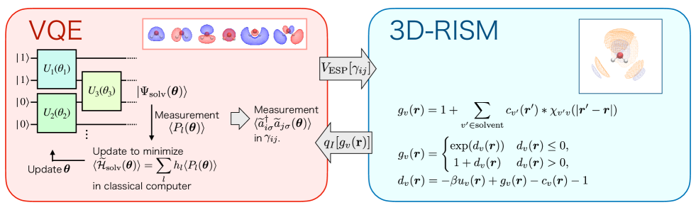
Figure 1: The scheme of 3D-RISM-VQE.

VQE and 3D-RISM computations are repeated to obtain the self-consistent solvent charge density and solute density matrix. In 3D-RISM-VQE, the solute density matrix can be obtained from measurements. The density matrix ${\bm{D}}$ is given by the follows:

$$D_{\alpha\beta}=\sum_{i,j}C_{\alpha i}\gamma_{ij}C_{j\beta}^{*},$$ (12)

where $C_{\alpha i}$ is the coefficient of atomic orbital $\chi_{\alpha}$ in the $i$-th molecular orbital. The one electron reduced density matrix (1-RDM) ${\bm{\gamma}}$ is represented as follows:

$$\gamma_{ij}=\begin{cases}\sum_{\sigma}\langle\widetilde{a}_{i\sigma}^{\dagger}\widetilde{a}_{j\sigma}({\bm{\theta}})\rangle&\textrm{(active space)}\\ 2\delta_{ij}&\textrm{(core)}\\ 0&\textrm{(else)},\end{cases}$$ (13)

where $a_{i\sigma}^{\dagger}$ and $a_{i\sigma}$ are the creation and annihilation operators of the spin orbital $i\sigma$. The value of ${\bm{\gamma}}$ in active space can be obtained by measurements of the expectation value $\sum_{\sigma}\langle\widetilde{a}_{i\sigma}^{\dagger}\widetilde{a}_{j\sigma}({\bm{\theta}})\rangle$ via a qubit representation using a quantum computer.

We summarize to show the self-consistent scheme of the 3D-RISM-VQE in Figure 1. The expectation value $\langle\mathcal{\widetilde{H}}_{\rm solv}({\bm{\theta}})\rangle$ is minimized with respect to the rotational angle ${\bm{\theta}}$ of the quantum circuit. Using the variationally optimized wave function, the value of 1-RDM in Eq. (13) is computed, and $V_{\rm ESP}({\bm{r}}_{I})$ is prepared for 3D-RISM calculations. To prepare $\mathcal{H}_{\rm solv}$, the 3D-RISM equation (Eq. (3)) and a closure relation are solved to obtain $g_{v}({\bm{r}})$ and $\Delta\mu$. $\mathcal{H}_{\rm solv}$ is updated using the new solvent charge density $q_{I}$. Finally, the Helmholtz energy of the 3D-RISM-VQE can be obtained using the self-consistent procedure between VQE and 3D-RISM calculations.

II.3 $L^{1}$-norm from the Pauli-operator formed Hamiltonian

The $L^{1}$-norm of the $L$-dimensional vector ${\bm{h}}=[h_{1}\,h_{2}\,\cdots\,h_{L}]\in\mathbb{R}^{L}$, which is a coefficient vector of the qubit-represented Hamiltonian such as Eq. (11), is defined as follows Berry et al. (2020):

$$\lambda:=\|{\bm{h}}\|_{1}=\sum_{l=1}^{L}|h_{l}|.$$ (14)

In this paper, $L^{1}$-norm values do not include the coefficient of the identity operator $I$.

III Computational Details

We have implemented the 3D-RISM-VQE method using PySCFSun et al. (2020, 2018), OpenFermionMcClean et al. (2020), and QulacsSuzuki et al. (2021) libraries. PySCF was used to calculate molecular integrals, natural orbitals, and second-quantized electronic Hamiltonians. OpenFermion was used to transform a fermionic operator into a qubit representation. We employed the Jordan–Wigner (JW) transformation for fermion-to-qubit mapping. Qulacs was employed as a quantum circuit emulator. We utilized the disentangled unitary coupled-cluster singles and doubles (UCCSD) ansatzKutzelnigg (1982); Kutzelnigg and Koch (1983); Kutzelnigg (1985); Bartlett et al. (1989); Kutzelnigg (1991); Taube and Bartlett (2006); Peruzzo et al. (2014); Evangelista et al. (2019) for VQE. The active space of VQE is denoted as ($m$e, $n$o), where $m$ and $n$ are the number of electrons and spatial orbitals, respectively.

3D-RISM calculations were performed using the RISMiCal program packageYoshida (2020). 3D-RISM uses Kovalenko–Hiraka (KH) closureKovalenko and Hirata (1999); Sato et al. (2000), and water as the solvent. The number of reference points for the 3D-RISM calculation is given as a three-dimensional grid. For each direction of the $x$, $y$, and $z$-axis, $128$ points were generated with $\delta=0.25$ Å spacing. TIP3PJorgensen et al. (1983) with modified hydrogen parameters and OPLS-AAJorgensen and Gao (1986) models was used for H₂O and NH${}_{4}^{+}$, respectively, regarding the Lennard-Jones parameters for the solutes. The modified hydrogen parameters were $\sigma_{H}=0.4$ Åand $\varepsilon_{H}=192.5$ J mol^-1.

The geometry of the solutes was optimized using the Gaussian16 package Revision CFrisch et al. (2016). Geometry optimizations were performed at the B3LYP/6-31G* level using the PCM. For Edminston–Ruedenberg (ER) localization in $L^{1}$-norm analysis, we use a fortran code fcidump_rotation.f90, which is part of the NECI program packageGuther et al. (2020). We performed the ER localization with all occupied and virtual orbitals, and a convergence criterion was $1.0\times 10^{-6}$.

Three-dimensional molecular figures of the distribution functions of the solvent and molecular orbitals were visualized using VMDHumphrey et al. (1996).

IV Result and discussion

First, we show the distribution functions of solvent water $g_{v}({\bm{r}})$, which is self-consistently determined for the electronic ground-state of the solute water molecule. Second, we discuss the potential and Helmholtz energy curves of a NaCl molecule in water. Next, the Helmholtz energy and the related quantities of H₂O and NH${}_{4}^{+}$ in water were investigated. Finally, the $L^{1}$-norms of the solvated Hamiltonian in a qubit representation are shown to elucidate the degree to which the solvent effect influences the difficulty of quantum computations.

IV.1 Spatial distribution of solvent

To determine the solvation structure intuitively, we first visualized its three-dimensional distribution functions $g_{v}({\bm{r}})$ in Figure 2, resulting from the 3D-RISM-VQE(8e, 6o) calculation with the 6-31G* basis set. The arched bilayered solvent shell near the solute oxygen and on the opposite side of the two hydrogens of the solute can be identified; the inside layer is $g_{{\rm H}}({\bm{r}})$ and the outside is $g_{{\rm O}}({\bm{r}})$. Two other distributions of $g_{{\rm O}}({\bm{r}})$ and $g_{{\rm H}}({\bm{r}})$ are situated around the two hydrogen atoms and on the opposite side of the solute oxygen.

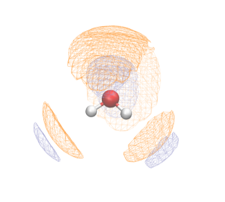
Figure 2: Spatial distribution functions of water around H₂O. Orange and ice-blue colorations correspond to $g_{{\rm O}}({\bm{r}})$ and $g_{{\rm H}}({\bm{r}})$. Isovalues are 2.4 and 1.8, respectively.

Contour plots of the distribution functions $g_{v}({\bm{r}})$ are shown in Figure 3. The solute water molecule is positioned on the $x=0$ plane, and the distribution functions on the same plane are shown. The resulting distribution functions $g_{v}({\bm{r}})$ are reliable compared to previous 3D-RISM studiesBeglov and Roux (1997). Figure 3 (a) shows the distribution when $v={\rm O}$ and the two significant peaks exist, symmetrically, close to the solute H and on the other side of the solute O across from the solute H. These peaks occur because solute H atoms are polarized positively and attract the negatively charged O site via electrostatic interaction. A small peak around $(y,z)=(0,3)$ is related to the distribution of solvent H atoms.

(a) $g_{{\rm O}}({\bm{r}})$

(b) $g_{{\rm H}}({\bm{r}})$

Figure 3: Contour plot showing the spatial distributions of water around an H₂O molecule on the $x=0$ plane. The diameter of the solute atoms is $\sigma_{uv}$.

Figure 3 (b) shows that the distribution $g_{{\rm H}}({\bm{r}})$ indicating a sharp peak around $(y,z)=(0,1.5)$. This peak indicates that the negatively polarized solute O atom is attracted to the solvent H sites, which are positively charged. The small peak of $g_{{\rm O}}({\bm{r}})$ around $(y,z)=(0,3)$ is related to this prominent peak because of intramolecular correlation. Similarly, the two small peaks of $g_{{\rm H}}({\bm{r}})$ in the lower part of the figure are correlated to the two large peaks of $g_{{\rm O}}({\bm{r}})$. Therefore, 3D-RISM-VQE can calculate appropriate distribution functions of solvent water.

IV.2 Energy curves of NaCl

Figure 4 shows the potential energy curve of NaCl dissociation, where the points were calculated at 0.25 Å intervals. The cc-pVTZ basis set was chosen. The potential energy is defined as the sum of the expectation value of $\mathcal{H}_{\rm iso}$ and the solute–solvent binding energyOkamoto et al. (2019). We employed the natural orbitals of CCSD to include electron correlation effectively. The potential energies of 3D-RISM-VQE(2e, 2o) stabilize at approximately 0.15 eV at 3.00 Å  and 0.18 eV at 7.00 Å  compared with the 3D-RISM-SCF calculations using restricted Hartree-Fock (RHF), termed 3D-RISM-RHF. The energy difference between them is slightly larger in the region where the interatomic distance $R$ is long. The curve of 3D-RISM-VQE(6e, 8o) becomes more stable at approximately 2.7 eV as a result of the electron correlation effect. The largest stabilization is 2.76 eV at 2.00 Å.

The potential energy curve does not exhibit any minima in this region. In the gas phase, the two ionic species may have made contact via electrostatic interactionsZeiri and Balint-Kurti (1983). On the other hand, in water, this figure shows the dissociative features of NaCl without forming a chemical bond from the viewpoint of total potential energy. This agrees with the conclusions of the one-dimensional RISM-MCSCF calculationsOkamoto et al. (2019).

Figure 5 shows the Helmholtz energy curve of NaCl. Unlike the potential energy, an energy minimum around $R/{\rm\AA}=2.50$ to $2.75$ is present. At this bond length, the ions are considered to be in contact. In the (2e, 2o) case, the Helmholtz energy difference from 3D-RISM-RHF is nearly constant, about $-0.17$ to $-0.18$ eV. In the (6e, 8o) case, the difference is also nearly constant in the R/Å$\geq$ 2.75 region, about $-2.71$ to $-2.72$ eV. The difference in the tightly contact ion pair region becomes slightly larger, and the maximum is $-2.78$ eV at 2.00 Å. Stabilizations in the two VQEs are almost independent of the interatomic distance because the natural orbitals in the active space are localized in the Cl atom.

Another shallow minimum is found at around 5.00 Å in the two 3D-RISM-VQE and -RHF calculations. At this minimum, the two ions are not in contact, but the solvent waters are distributed between them. This is a feature of the so-called solvent-shared ion pairHirata (2003); Brini et al. (2017); Yao and Kanai (2018).

The Helmholtz energy of the ionic pair dissociation determined by our calculations is not lower than that of the minimum of the contact ions; this agrees with the results of an ab initio molecular dynamics studyYao and Kanai (2018), although the statistical ensemble is not the same as RISM.

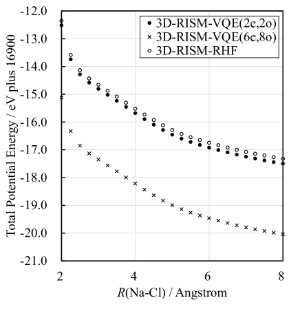
Figure 4: Potential energy curve of NaCl calculated by combined 3D-RISM and VQE or restricted Hartree-Fock (RHF), respectively.

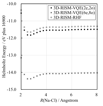
Figure 5: The Helmholtz energy curve of NaCl calculated by combined 3D-RISM and VQE or RHF, respectively.

IV.3 H₂O and NH${}_{4}^{+}$

IV.3.1 Helmholtz energies

Table 1 shows the values of the Helmholtz energy $\mathcal{A}$, the free energy components $\langle\mathcal{H_{\rm iso}}({\bm{\theta}})\rangle$ and $\Delta\mu$, and the expectation value of the solvated Hamiltonian $\langle\mathcal{H_{\rm solv}}({\bm{\theta}})\rangle$. This table shows that the solute energy $\langle\mathcal{H_{\rm iso}}({\bm{\theta}})\rangle$ predominantly contributes to the free energy $\mathcal{A}$. The value of $\mathcal{A}$ decreases systematically in both molecules as the basis set or active space becomes larger. The energy of the solute $\langle\mathcal{H_{\rm iso}}({\bm{\theta}})\rangle$ has the same trend as $\mathcal{A}$, and the contribution of $\Delta\mu$ to the free energy is minimal.

As the active space expands, the value of the solvation free energy $\Delta\mu$ increases less than the decrease of $\langle\mathcal{H_{\rm iso}}({\bm{\theta}})\rangle$. It is considered that the electronic interaction between solute and solvent is given by the multiplication of the distributions of the solvent and electrons and a small part of the electrons move into virtual orbitals to stretch the distribution via electronic correlation. However, it should be reiterated that the contribution of $\Delta\mu$ is much smaller than that of $\langle\mathcal{H_{\rm iso}}({\bm{\theta}})\rangle$.

The value of $\langle\mathcal{H_{\rm solv}}({\bm{\theta}})\rangle$ is comparable to that of $\langle\mathcal{H_{\rm iso}}({\bm{\theta}})\rangle$, and the contribution of solute–solvent interaction $\langle\mathcal{V_{\rm solv}}({\bm{\theta}})\rangle$ is minor in comparison. Regarding $\langle\mathcal{H_{\rm solv}}({\bm{\theta}})\rangle$, there was no clear increasing or decreasing trend against the sizes of the basis set and the active space.

Table 1: Helmholtz energy components and expectation values of solvated Hamiltonians of H₂O and NH${}_{4}^{+}$ in aqueous solution (in a.u.).

Molecule	Basis set	Method	$\mathcal{A}$	$\langle\mathcal{H}_{\rm iso}({\bm{\theta}})\rangle$	$\Delta\mu$	$\langle\mathcal{H}_{\rm solv}({\bm{\theta}})\rangle$
H2O	STO-3G	3D-RISM-VQE(2e, 2o)	$-$74.9651	$-$74.9651	0.0001	$-$75.3240
		3D-RISM-VQE(8e, 6o)	$-$75.0138	$-$75.0152	0.0014	$-$75.3489
	6-31G	3D-RISM-VQE(2e, 2o)	$-$75.9988	$-$75.9781	$-$0.0207	$-$76.6014
		3D-RISM-VQE(8e, 6o)	$-$76.0086	$-$75.9905	$-$0.0181	$-$76.5833
	6-31G*	3D-RISM-VQE(2e, 2o)	$-$76.0178	$-$76.0044	$-$0.0134	$-$76.5387
		3D-RISM-VQE(8e, 6o)	$-$76.0271	$-$76.0159	$-$0.0112	$-$76.5225
NH${}_{4}^{+}$	STO-3G	3D-RISM-VQE(2e, 2o)	$-$55.9672	$-$55.8685	$-$0.0987	$-$53.6213
		3D-RISM-VQE(4e, 4o)	$-$55.9693	$-$55.8706	$-$0.0987	$-$53.6235
		3D-RISM-VQE(6e, 6o)	$-$55.9977	$-$55.8990	$-$0.0986	$-$53.6509
		3D-RISM-VQE(8e, 8o)	$-$56.0462	$-$55.9478	$-$0.0983	$-$53.7024
	6-31G	3D-RISM-VQE(2e, 2o)	$-$56.6154	$-$56.5161	$-$0.0993	$-$54.2678
		3D-RISM-VQE(4e, 4o)	$-$56.6159	$-$56.5166	$-$0.0993	$-$54.2670
		3D-RISM-VQE(6e, 6o)	$-$56.6235	$-$56.5244	$-$0.0991	$-$54.2764
		3D-RISM-VQE(8e, 8o)	$-$56.6365	$-$56.5376	$-$0.0989	$-$54.2906
	6-31G*	3D-RISM-VQE(2e, 2o)	$-$56.6287	$-$56.5294	$-$0.0994	$-$54.2806
		3D-RISM-VQE(4e, 4o)	$-$56.6293	$-$56.5299	$-$0.0994	$-$54.2798
		3D-RISM-VQE(6e, 6o)	$-$56.6366	$-$56.5373	$-$0.0992	$-$54.2882
		3D-RISM-VQE(8e, 8o)	$-$56.6492	$-$56.5502	$-$0.0990	$-$54.3030

IV.3.2 Evaluation of 1-norm

The $L^{1}$-norm values of the Hamiltonians with and without solvent effect are compared in Table 2. The values of $\lambda$ by Bravyi–Kitaev (BK) and symmetry conserving BK transformations are the same as those obtained by JW transformation. Table 2 shows that the $\lambda$ value using canonical molecular orbital (CMO) is almost unchanged when adding the solvent effect; the ER-localized orbital indicates a similar trend. This can be explained if the expectation values of $\mathcal{H_{\rm solv}}$ and $\mathcal{H_{\rm iso}}$ are comparable, as shown in Table 1, and implies that a quantum computer could perform quantum chemical calculations of a molecule in solution at practically the same cost as in gas.

Koridon et al. demonstrated that orbital localizations could decrease the $L^{1}$-norm value compared to CMOKoridon et al. (2021). However, the reduction effect is not apparent in our analysis. Our molecules are small, and the difference between delocalized and localized orbitals is also small.

Table 2: Values of $\lambda$ with the methods for molecules in gas (g) and in solution (s).

Molecule	Method	STO-3G				6-31G				6-31G*
		CMO	s/g ratio	ER	s/g ratio	CMO	s/g ratio	ER	s/g ratio	CMO	s/g ratio	ER	s/g ratio
H2O	RHF	72		80		160		139		327		365
	3D-RISM-VQE(2e, 2o)	72	100.3%	81	100.3%	153	96.0%	139	99.5%	326	99.8%	364	99.8%
	3D-RISM-VQE(8e, 6o)	72	100.3%	81	100.3%	153	96.1%	139	100.0%	328	100.3%	364	99.9%
NH${}_{4}^{+}$	RHF	73		78		230		178		475		429
	3D-RISM-VQE(2e, 2o)	71	97.2%	76	97.4%	233	101.5%	181	101.9%	480	101.0%	434	101.1%
	3D-RISM-VQE(4e, 4o)	71	97.3%	76	97.4%	233	101.6%	181	101.8%	480	101.0%	434	101.1%
	3D-RISM-VQE(6e, 6o)	71	97.4%	76	97.4%	234	101.9%	180	101.5%	481	101.1%	434	101.2%
	3D-RISM-VQE(8e, 8o)	71	97.2%	76	97.4%	233	101.5%	181	101.9%	480	101.0%	434	101.1%

V Conclusion

3D-RISM-VQE combines VQE and 3D-RISM-SCF theory. The electronic structure of the solute is affected by the countless number of solvent molecules, and the electrostatic interaction term from the solvent is added into the solute Hamiltonian in a QM/MM manner. Using an analytical treatment of the solvent distribution, the present method does not include errors from the solvent configuration sampling.

We have demonstrated the spatial distribution functions $g_{v}({\bm{r}})$ around an H₂O, showing that the present method can give reasonable distributions of solvent water. We have also shown the potential and Helmholtz energy curves of NaCl. The dissociative feature of the potential energy curve, previously shown by one-dimensional RISM-MCSCFOkamoto et al. (2019), was successfully reproduced. The minimum of the Helmholtz energy curve corresponds to the ions in contact. A dissociation of molecular species is one of the essential themes that can cause static electronic correlation. In the case of H₂O and NH${}_{4}^{+}$, the Helmholtz energy components and the expectation values of the solvated Hamiltonians were investigated. The expectation values of the solute Hamiltonian are dominant in both the Helmholtz energy and the expectation value of the solvated Hamiltonian. Finally, we analyzed the $L^{1}$-norm of the modified Hamiltonian in a qubit representation, which is a key to quantifying the algorithmic scaling of various quantum algorithms. The $L^{1}$-norm value of the solvated Hamiltonian is almost the same as that in the gas phase, implying that the efficiency of quantum chemical computations including solvent effects on a quantum computer are virtually the same as those in gas phases.