Structure of electrolyte solutions at non-uniformly charged surfaces on a variety of length scales

Abstract

The structures of dilute electrolyte solutions close to non-uniformly charged planar substrates are systematically studied within the entire spectrum of microscopic to macroscopic length scales by means of a unified classical density functional theory (DFT) approach. This is in contrast to previous investigations, which are applicable either to short or to long length scales. It turns out that interactions with microscopic ranges, e.g., due to the hard cores of the fluid molecules and ions, have negligible influence on the formation of non-uniform lateral structures of the electrolyte solutions. This partly justifies the Debye-Hückel approximation schemes applied in previous studies of that system. In general, a coupling between the lateral and the normal fluid structures leads to the phenomenology that, upon increasing the distance from the substrate, less details of the lateral non-uniformities contribute to the fluid structure, such that ultimately only large-scale surface features remain relevant. It can be expected that this picture also applies to other fluids characterized by several length scales.

I Introduction

Historically, the theoretical study of solid-fluid interfaces has naturally started with the investigation of idealized surfaces with laterally uniform properties Gibbs ; Helmholtz1879 ; Gouy1909 ; Gouy1910 ; Chapman1913 ; Grahame1947 instead of realistic models of surfaces with geometrical, chemical, or electrical non-uniformities. This approach was justified, on the one hand, by the initial lack of knowledge about the microscopic structure of real surfaces, and, on the other hand, by the computational advantages gained from exploiting lateral symmetries. However, in particular in the context of electrochemistry and colloidal science, efforts have been made to include surface non-uniformities into the theoretical description. A pioneering contribution is due to Richmond Richmond1974 ; Richmond1975 , who studied the effective interaction of two parallel planar dielectric bodies with non-uniform surface charge distributions mediated by a dilute electrolyte solution in between, assuming that the linearized Poisson-Boltzmann (Debye-Hückel) approximation Debye1923 (see also Refs. Russel1989 ; McQuarrie2000 ; Hunter2001 ) is applicable. In recent years the issue of electrolyte solutions close to non-uniformly charged substrates within the Debye-Hückel approximation BenYaakov2013 ; Ghosal2017 ; Mussotter2018 ; Sherwood2020 , (non-linearized) Poisson-Boltzmann theory Adar2016 ; Adar2018 , as well as statistical field theory Naji2010 ; Naji2014 ; Ghodrat2015a ; Ghodrat2015b ; Naji2018 has been addressed intensively (see also the review in Ref. Adar2017 ). These studies are focused on large length scales, either by ignoring the microscopic fluid structure of the electrolyte solution or by modelling its long-ranged structure within a square gradient approximation (see Ref. Mussotter2018 ). Moreover, microscopic approaches, e.g., Monte Carlo (MC) simulations Bakhshandeh2015 ; Zhou2017 or classical density functional theory (DFT) McCallum2017 ; Mussotter2020 , have been used. But, due to technical reasons, theses studies were limited to rather small systems and special types of surface charge non-uniformities. Thus an approach is missing which exhibits the accuracy of a DFT combined with the efficiency of a Debye-Hückel approximation, in order to span the whole range from microscopic to macroscopic length scales.

The present study suggests a step in this direction. This novel method consists of a quadratic expansion of the density functional not about the bulk profiles (as within the Debye-Hückel approximation), but about the profiles of a planar-symmetric (i.e., quasi one-dimensional) system. The surprising observation is, that microscopic hard-core contributions turn out to be quantitatively irrelevant for the formation of the lateral structure. In this respect, disregarding the size of the fluid molecules and ions by using the Debye-Hückel approximation for laterally non-uniform modes, as done in many previous studies, is justified. However, the present investigation suggests, that, in contrast to those previous studies, the Debye-Hückel approximation should not be used for the planar-symmetric contributions, which require more sophisticated descriptions including, e.g., finite size effects.

Our contribution is structured as follows: Section II describes the considered model of an electrolyte solution in contact with a non-uniformly charged substrate and the formalism to infer the structural quantities. Results concerning the number density profiles in the normal and in the lateral directions as well as concerning the interfacial tension as function of the length scales of the lateral non-uniformities are presented and discussed in Sec. III. Conclusions about the general structural features of electrolyte solutions in contact with non-uniformly charged substrates are summarized in Sec. IV.

II Model and formalism

II.1 Non-uniformly charged substrate

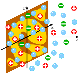
Figure 1: A planar, non-uniformly charged substrate with negatively charged (bright, yellow) and charge-neutral (dark, brown) regions is in contact with a dilute univalent electrolyte solution (solvent blue, cations red, anions green). The $x$-$y$-plane of a three-dimensional Cartesian coordinate system coincides with the substrate surface, whereas the $z$-direction points in normal direction towards the bulk of the electrolyte solution.

We consider a flat substrate with dielectric constant $\varepsilon_{s}$ the surface of which coincides with the $x$-$y$-plane of a three-dimensional Cartesian coordinate system; the $z$-direction is pointing towards the fluid at $z>0$ (see Fig. 1). The substrate is non-uniformly charged with the surface charge density $\sigma(\mathbf{u})$ at the lateral position $\mathbf{u}=(x,y)$. In the present study periodic surface charge densities of the form

$$\sigma(\mathbf{u})=\sum_{k,\ell\in\mathbb{Z}}\widehat{\sigma}_{k\ell}\ \exp\left(\frac{2\pi i}{L}(kx+\ell y)\right),$$ (1)

are analyzed. The Fourier coefficients $\widehat{\sigma}_{k\ell}\in\mathbb{C}$, which fulfill the constraints $\widehat{\sigma}_{k,\ell}^{*}=\widehat{\sigma}_{-k,-\ell}$ for $\sigma(u)\in\mathbb{R}$, and the lateral length scale $L>0$ are free parameters. It will turn out that the periodicity of the lateral surface charge distribution is of no physical relevance, but it is technically convenient.

II.2 Charged hard spheres

The charged substrate is in contact with a dilute univalent electrolyte solution comprising three species of charged hard spheres: the solvent (species $i=0$), cations (species $i=+$), and anions (species $i=-$). Each species $i$ is characterized by its hard-core radius $R_{i}$ and the valency $Z_{i}$ with $Z_{0}=0,Z_{+}=1,Z_{-}=-1$. For simplicity, all radii are chosen to be equal, i.e., $R_{0}=R_{+}=R_{-}=:R$. The bulk number densities of the electrolyte solution are given by $\overline{\varrho}_{0}$ and $\overline{\varrho}_{+}=\overline{\varrho}_{-}=:I$, which is called the ionic strength. This leads to the packing fraction $\displaystyle\eta=\frac{4\pi}{3}R^{3}(\overline{\varrho}_{0}+2I)$. From the Bjerrum length $\displaystyle\ell_{B}:=\frac{\beta e^{2}}{4\pi\varepsilon_{0}\varepsilon_{f}}$, which is expressed in terms of the thermal energy $\beta^{-1}=k_{B}T$, the elementary charge $e$, the vacuum electric permittivity $\varepsilon_{0}$, and the fluid dielectric constant $\varepsilon_{f}$, one obtains the Debye length $\kappa^{-1}$ with $\kappa^{2}=8\pi\ell_{B}I$.

II.3 Density functional method

Close to the substrate the number density profile $\varrho_{i}(\mathbf{r})$ of the fluid species $i$ varies as function of the position $\mathbf{r}=(x,y,z)=(\mathbf{u},z)$, whereas $\varrho_{i}(\mathbf{u},z\to\infty)\to\overline{\varrho}_{i}$. The set of all three number density profiles is abbreviated by $\varrho:=(\rho_{0},\rho_{+},\rho_{-})$. The equilibrium number density profiles minimize the grand potential density functional $\Omega[\varrho]$ Evans1979 ; Evans1990 ; Evans1992 , which, in the present investigation, is approximated by

$$\beta\Omega[\varrho]=\int\mathrm{d}^{3}r\bigg{\{} \ \sum_{i}\varrho_{i}(\mathbf{r})\left[\ln\left(\frac{\varrho_{i}(\mathbf{r})}{\zeta_{i}}\right)-1+\beta V_{i}(z)\right]$$

$$\ +\Phi(n(\mathbf{r}))+\frac{\beta\varepsilon_{0}\varepsilon(z)}{2}\left(\nabla\psi(\mathbf{r})\right)^{2}\bigg{\}}.$$ (2)

Here and in the following the common convention is in place that a $d$-dimensional integration runs over $\mathbb{R}^{d}$ unless the integration domain is specified. Equation (2) is to be understood as an asymptotic relation in the thermodynamic limit, i.e., first all calculations are performed in a finite domain which is extended to $\mathbb{R}^{3}$ subsequently. The thermodynamic limit is guaranteed to exist, i.e., $\beta\Omega[\varrho]$ scales as the volume of the system, because the number density profiles $\rho_{i}(\mathbf{r})$ are bounded due to the imposed lateral periodicity of the system (see Eq. (1)) and due to the bulk limits $\varrho_{i}(z\to\pm\infty)$. In Eq. (2), $\displaystyle\zeta_{i}=\Lambda_{i}^{-3}\exp(\beta\mu_{i})$, with the thermal wavelength $\Lambda_{i}$ and the chemical potential $\mu_{i}$, denotes the (bulk) fugacity of species $i\in\{0,+,-\}$. The hard-wall potential

$$V_{i}(z)=\begin{cases}\infty&\text{for $z\leq R_{i}$}\\ 0&\text{for $z>R_{i}$}\end{cases}$$ (3)

implies that the fluid particles cannot penetrate into the substrate. The hard-core interaction among the fluid particles is described in terms of the White-Bear (mark I) excess free energy Roth2002 , which is given by an excess free energy density $\Phi(n(r))$ expressed in terms of ten weighted densities

$$n_{\alpha}(\mathbf{r})=\sum_{i}\int\mathrm{d}^{3}r^{\prime}\,\omega_{\alpha,i}(\mathbf{r}-\mathbf{r^{\prime}})\varrho_{i}(\mathbf{r^{\prime}})$$ (4)

that are indexed by $\alpha$ and that follow from the number density profiles $\varrho_{i}$ via the weight functions $\omega_{\alpha,i}$. The electrostatic potential $\psi(\mathbf{r})$ fulfills Gauß’s law

$$\nabla\cdot\left(-\varepsilon_{0}\varepsilon(z)\nabla\psi(\mathbf{r})\right)=\sigma(\mathbf{u})\delta(z)+Q(\mathbf{r}),$$ (5)

where $Q(\mathbf{r}):=e\sum_{i}Z_{i}\varrho_{i}(\mathbf{r})$ and

$$\varepsilon(z)=\begin{cases}\varepsilon_{s}&\text{for $z\leq 0$}\\ \varepsilon_{f}&\text{for $z>0$}\end{cases}$$ (6)

with the boundary conditions

$$\frac{\partial\psi}{\partial z}\Big{|}_{(\mathbf{u},z=-\infty)} =0,$$ (7)

$$-\varepsilon_{0}\left(\varepsilon_{f}\frac{\partial\psi}{\partial z}\Big{|}_{(\mathbf{u},z=0^{+})}-\varepsilon_{s}\frac{\partial\psi}{\partial z}\Big{|}_{(\mathbf{u},z=0^{-})}\right) =\sigma(\mathbf{u}),$$ (8)

$$\psi\Big{|}_{(\mathbf{u},z=\infty)} =0$$ (9)

for all $\mathbf{u}\in\mathbb{R}^{2}$ in lateral direction. In order to guarantee the existence of the thermodynamic limit we consider a globally charge-neutral system; actually Lebowitz and Lieb have shown that slightly weaker but rather artificial conditions would also suffice Lebowitz1969 . Globally charge-neutral systems exhibit the gauge symmetry $\psi\mapsto\psi+\text{const}$, which is used to fix the value of the electrostatic potential at $z=\infty$ by means of the Dirichlet boundary condition (see Eq. (9)). This implies the Neumann boundary condition $\displaystyle\frac{\partial\psi}{\partial z}\Big{|}_{(\mathbf{u},z=\infty)}=0$. For a globally charge-neutral system the electric displacement $\displaystyle-\varepsilon_{0}\varepsilon\frac{\partial\psi}{\partial z}$ has to be the same at $z=-\infty$ and at $z=\infty$, which leads to Eq. (7). Finally, Eq. (8), which is obtained by integrating Eq. (5) over an infinitessimally small box around the point $(\mathbf{u},z=0)$, describes the discontinuity of the electric displacement at the charged surface $z=0$.

The equilibrium number density profiles $\varrho_{i}(\mathbf{r})$ vanish for $z\leq R_{i}$ due to the hard wall (see Eq. (3)), whereas for $z>R_{i}$ they fulfill the Euler-Lagrange equations

$$0= \ \frac{\delta\beta\Omega}{\delta\rho_{i}(\mathbf{r})}[\varrho]$$

$$= \ \ln\left(\frac{\varrho_{i}(\mathbf{r})}{\zeta_{i}}\right)+\beta eZ_{i}\psi(\mathbf{r})+$$

$$\ \sum_{\alpha}\int\mathrm{d}^{3}r^{\prime}\,\frac{\partial\Phi}{\partial n_{\alpha}}(n(\mathbf{r^{\prime}}))\,\omega_{\alpha,i}(\mathbf{r^{\prime}}-\mathbf{r}).$$ (10)

The set of equations (5) and (7)–(10) is technically too demanding to be solvable numerically for an arbitrary lateral length scale $L$. In order to proceed, Eqs. (5) and (7)–(10) are first solved for the laterally uniform charge distribution $\sigma^{(1)}:=\widehat{\sigma}_{00}$, which renders the quasi one-dimensional number density profiles, the weighted densities, and the electrostatic potential denoted as $\varrho_{i}^{(1)}(z)$, $n_{\alpha}^{(1)}(z)$, and $\psi^{(1)}(z)$, respectively.

The quadratic expansion of the density functional in Eq. (2) about $\varrho_{i}^{(1)}(z)$ in terms of $\Delta\varrho_{i}(\mathbf{u},z):=\varrho_{i}(\mathbf{r}=(\mathbf{u},z))-\varrho_{i}^{(1)}(z)$ yields the approximation $\Omega[\varrho]\approx\Omega[\varrho^{(1)}]+\Delta\Omega[\Delta\varrho]$ with $\Delta\varrho:=(\Delta\varrho_{0},\Delta\varrho_{+},\Delta\varrho_{-})$, where

$$\beta\Delta\Omega[\Delta\varrho]=$$ (11)

$$\ \frac{1}{2}\int\mathrm{d}^{3}r\,\bigg{(}\sum_{i}\frac{(\Delta\varrho_{i}(\mathbf{r}))^{2}}{\varrho_{i}^{(1)}(z)}+\beta\varepsilon_{0}\varepsilon(z)\,(\nabla\Delta\psi(\mathbf{r}))^{2}+$$

$$\ \phantom{\frac{1}{2}\int\mathrm{d}^{3}r\,\bigg{(}}\sum_{\alpha,\alpha^{\prime}}\frac{\partial^{2}\Phi}{\partial n_{\alpha}\partial n_{\alpha^{\prime}}}(n^{(1)}(z))\,\Delta n_{\alpha}(\mathbf{r})\Delta n_{\alpha^{\prime}}(\mathbf{r})\bigg{)}$$

with $\Delta n_{\alpha}(\mathbf{u},z)=n_{\alpha}(\mathbf{u},z)-n^{(1)}_{\alpha}(z)$ and $\Delta\psi(\mathbf{u},z)=\psi(\mathbf{u},z)-\psi^{(1)}(z)$. (Note that here “$\Delta$” is not the Laplace operator $\mathbf{\nabla}^{2}$).

The equilibrium profiles $\Delta\rho_{i}(\mathbf{r})$ fulfill the Euler-Lagrange equations

$$0= \ \frac{\delta\beta\Delta\Omega}{\delta\Delta\rho_{i}(\mathbf{r})}[\Delta\varrho]$$

$$= \ \frac{\Delta\varrho_{i}(\mathbf{r})}{\rho^{(1)}_{i}(z)}+\beta eZ_{i}\,\Delta\psi(\mathbf{r})+$$ (12)

$$\ \sum_{\alpha,\alpha^{\prime}}\int\mathrm{d}^{3}r^{\prime}\,\frac{\partial^{2}\Phi}{\partial n_{\alpha}\partial n_{\alpha^{\prime}}}(n^{(1)}(z^{\prime}))\,\omega_{\alpha,i}(\mathbf{r^{\prime}}-\mathbf{r})\Delta n_{\alpha^{\prime}}(\mathbf{r^{\prime}})$$

for $z>R_{i}$.

Introducing the lateral Fourier-transform

$$\widehat{f}(\mathbf{q}):=\int\mathrm{d}^{2}u\,f(\mathbf{u})\exp(-i\mathbf{q}\cdot\mathbf{u}),\quad\mathbf{q}\in\mathbb{R}^{2},$$ (13)

for functions $f(\mathbf{u})$ of the lateral coordinates $\mathbf{u}\in\mathbb{R}^{2}$, from Eq. (12) one obtains

$$0= \frac{\Delta\widehat{\varrho}_{i}(\mathbf{q},z)}{\rho^{(1)}_{i}(z)}+\beta eZ_{i}\,\Delta\widehat{\psi}(\mathbf{q},z)+$$ (14)

$$\sum_{\alpha,\alpha^{\prime}}\!\int\!\!\mathrm{d}z^{\prime}\!\frac{\partial^{2}\Phi}{\partial n_{\alpha}\partial n_{\alpha^{\prime}}}(n^{(1)}(z^{\prime}))\,\widehat{\omega}_{\alpha,i}(\mathbf{q},z^{\prime}\!-\!z)\Delta\widehat{n}_{\alpha^{\prime}}(\mathbf{q},z^{\prime})$$

for $z>R_{i}$ with

$$\Delta\widehat{n}_{\alpha}(\mathbf{q},z)=\sum_{i}\int\mathrm{d}z^{\prime}\,\widehat{\omega}_{\alpha,i}(\mathbf{q},z-z)\Delta\widehat{\varrho}_{i}(\mathbf{q},z^{\prime}).$$ (15)

Moreover, the lateral Fourier transformation of Gauß’s law (see Eq. (5)) leads, due to Eq. (6), to the Helmholtz equations

$$\frac{\partial^{2}\Delta\widehat{\psi}}{\partial z^{2}}(\mathbf{q},z)-|\mathbf{q}|^{2}\Delta\widehat{\psi}(\mathbf{q},z) =-\frac{\Delta\widehat{Q}(\mathbf{q},z)}{\varepsilon_{0}\varepsilon_{f}}$$

for $$z>0$$, (16)

$$\frac{\partial^{2}\Delta\widehat{\psi}}{\partial z^{2}}(\mathbf{q},z)-|\mathbf{q}|^{2}\Delta\widehat{\psi}(\mathbf{q},z) =-\frac{\Delta\widehat{Q}(\mathbf{q},z)}{\varepsilon_{0}\varepsilon_{s}}=0$$

for $$z<0$$, (17)

where $\displaystyle\Delta\widehat{Q}(\mathbf{q},z)=e\sum_{i}Z_{i}\Delta\widehat{\varrho}_{i}(\mathbf{q},z)$. Finally, the boundary conditions Eqs. (7)–(9) take the form

$$\frac{\partial\Delta\widehat{\psi}}{\partial z}\Big{|}_{(\mathbf{q},z=-\infty)} =0,$$ (18)

$$\varepsilon_{f}\frac{\partial\Delta\widehat{\psi}}{\partial z}\Big{|}_{(\mathbf{q},z=0^{+})}-\varepsilon_{s}\frac{\partial\Delta\widehat{\psi}}{\partial z}\Big{|}_{(\mathbf{q},z=0^{-})} =-\frac{\Delta\widehat{\sigma}(\mathbf{q})}{\varepsilon_{0}},$$ (19)

$$\Delta\widehat{\psi}\Big{|}_{(\mathbf{q},z=\infty)} =0.$$ (20)

Here $\Delta\widehat{\sigma}(\mathbf{q})$ is the lateral Fourier transform of the non-uniform contribution $\Delta\sigma(\mathbf{u}):=\sigma(\mathbf{u})-\sigma^{(1)}$ to the surface charge density.

The Helmholtz equation at $z<0$ (see Eq. (17)) and the Neumann boundary condition at $z=-\infty$ (see Eq. (18)) lead to solutions of the form $\displaystyle\Delta\widehat{\psi}(\mathbf{q},z)=\Delta\widehat{\psi}(\mathbf{q},0)\exp(|\mathbf{q}|z)$ for $z<0$. Then, from Eq. (19) one obtains the Robin boundary condition

$$\varepsilon_{f}\frac{\partial\Delta\widehat{\psi}}{\partial z}\Big{|}_{(\mathbf{q},z=0^{+})}-\varepsilon_{s}|\mathbf{q}|\Delta\widehat{\psi}\Big{|}_{(\mathbf{q},z=0)}=-\frac{\Delta\widehat{\sigma}(\mathbf{q})}{\varepsilon_{0}},$$ (21)

which, together with the Dirichlet boundary condition at $z=\infty$ (see Eq. (20)), determines the solution of the Helmholtz equation in Eq. (16). Note that in the first term of Eq. (21) the upper limit of $\displaystyle\frac{\partial\Delta\widehat{\psi}}{\partial z}$ occurs, because this quantity is discontinuous at the surface $z=0$ due to Eq. (19), whereas in the second term of Eq. (21) $\Delta\widehat{\psi}$ can be evaluated at the surface, because the electrosatic potential is continuous everywhere.

In the set of equations (14)–(21) the individual Fourier modes, indicated by $\mathbf{q}$, are decoupled, and the remaining $z$-coordinate normal to the substrate leads to a quasi one-dimensional problem, which can be efficiently solved numerically.

Moreover, any function $f(\mathbf{u})$ with $f(x+L,y)=f(x,y+L)=f(x,y)$ for all $\mathbf{u}=(x,y)\in\mathbb{R}^{2}$ can be written as

$$f(\mathbf{u}=(x,y))=\sum_{k,\ell\in\mathbb{Z}}f_{k\ell}\exp\left(\frac{2\pi i}{L}(kx+\ell y)\right)$$ (22)

with the the Fourier transform

$$\ \widehat{f}(\mathbf{q}=(q_{x},q_{y}))=$$

$$\ \sum_{k,\ell\in\mathbb{Z}}(2\pi)^{2}f_{k\ell}\,\delta\left(q_{x}-\frac{2\pi k}{L}\right)\delta\left(q_{y}-\frac{2\pi\ell}{L}\right),$$ (23)

which can be non-zero only for lateral wave numbers $\displaystyle\mathbf{q}=\mathbf{q}_{k\ell}:=\frac{2\pi}{L}(k,l)$ with $k,\ell\in\mathbb{Z}$. Therefore, the determination of the (approximate) equilibrium number density profiles $\varrho_{i}(\mathbf{r})$ merely requires to calculate the Fourier transforms $\Delta\widehat{\varrho}_{i}(\mathbf{q},z)$ as solutions of Eqs. (14)–(21) for $\mathbf{q}=\mathbf{q}_{k\ell}$ with $k,\ell\in\mathbb{Z}$.

II.4 Interfacial tension

Besides the profiles $\varrho_{i}(\mathbf{r})=\varrho_{i}^{(1)}(z)+\Delta\varrho_{i}(\mathbf{r})$, $Q(\mathbf{r})=Q^{(1)}(z)+\Delta Q(\mathbf{r})$, and $\psi(\mathbf{r})=\psi^{(1)}(z)+\Delta\psi(\mathbf{r})$, from Eqs. (14)–(21) the following discussion also addresses the interfacial tension $\gamma$ as a common surface quantity. Here it is defined w.r.t. the geometrical substrate surface at $z=0$. If $\gamma^{(1)}$ is the interfacial tension of a uniformly charged substrate with surface charge density $\sigma^{(1)}$, one obtains the deviation $\Delta\gamma:=\gamma-\gamma^{(1)}$ due to non-uniformities within the quadratic approximation (see Eq. (11)) as

$$\Delta\gamma=\frac{\Delta\Omega_{L}[\Delta\varrho]}{L^{2}}=\frac{1}{2L^{2}}\int\limits_{[0,L)^{2}}\mathrm{d}^{2}u\,\Delta\sigma(\mathbf{u})\Delta\psi(\mathbf{u},0),$$ (24)

where $\Delta\Omega_{L}$ means integration over $\mathbf{r}=(\mathbf{u},z)\in[0,L)^{2}\times\mathbb{R}$ in Eq. (11), i.e., over one lateral periodic image. This expression can be obtained by multiplying Eq. (12) with $\Delta\varrho_{i}(\mathbf{r})$, summing over $i$, integrating w.r.t. $\mathbf{r}$, and inserting the resulting equation into Eq. (11).

II.5 Parameters

The main focus of the present study is the dependence of the profiles $\varrho_{i}(\mathbf{r})$, $Q(\mathbf{r})$, and $\psi(\mathbf{r})$ as well as of the interfacial tension $\gamma$ on the characteristic length scale $L$ of the lateral charge non-uniformities. The remaining numerous model parameters are fixed to certain realistic values.

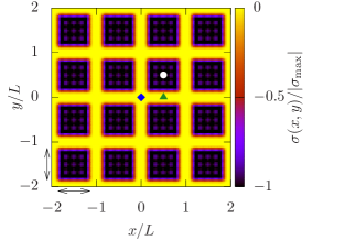
Figure 2: The non-uniform surface charge density $\sigma(x,y)$ comprising 25 Fourier modes (see Eq. (26)) considered in the present investigation is a continuous approximation of a substrate with half of its area being charge-neutral and the other half being made up of charged square patches of side length $L/\sqrt{2}$ (indicated by the double arrows in the lower left corner) with surface charge density $\sigma_{\text{max}}$. The restriction to a finite number of Fourier modes gives rise to slight artifacts such as smooth instead of step-like variations as well as undulations (see the apparent substructure in the dark square areas) instead of plateaus. The mean surface charge density is $\displaystyle\sigma^{(1)}=\frac{\sigma_{\text{max}}}{2}$. The charged patches are arranged on a (two-dimensional) square lattice with periodicity $L$, which sets the lateral length scale of this structure. Figure 3 displays the number density profiles $\varrho_{i}(\mathbf{u},z)$ along the $z$-direction at three lateral positions $\mathbf{u}=(x,y)$: $\mathbf{u}=(0,0)$ (blue diamond), $\mathbf{u}=(L/2,0)$ (green triangle), and $\mathbf{u}=(L/2,L/2)$ (white dot).

As a non-trivial surface structure we choose a two-dimensional square lattice with periodicity $L>0$ such that the surface charge density takes the constant value $\sigma_{\text{max}}$ for one half of the surface and $0$ for the other half. This leads to an average surface charge density $\displaystyle\sigma^{(1)}=\frac{\sigma_{\text{max}}}{2}$ and in Eq. (1) to the Fourier coefficients

$$\widehat{\sigma}_{k\ell}=\sigma^{(1)}\,(-1)^{k+\ell}\,\mathop{\mathrm{missing}}{sinc}\left(\frac{\pi k}{\sqrt{2}}\right)\,\mathop{\mathrm{missing}}{sinc}\left(\frac{\pi\ell}{\sqrt{2}}\right),$$ (25)

where the $\mathop{\mathrm{missing}}{sinc}$ function is defined as $\displaystyle\mathop{\mathrm{missing}}{sinc}(t)=\frac{\sin(t)}{t}$ for $t\not=0$ and $\mathop{\mathrm{missing}}{sinc}(t)=1$ for $t=0$. However, in order to limit the computational demand only Fourier modes with $|k|,|\ell|\leq 5$ are used here. The resulting surface charge density

$$\sigma(\mathbf{u}):=\sum_{k,\ell=-5}^{5}\widehat{\sigma}_{k\ell}\exp\left(\frac{2\pi i}{L}(kx+\ell y)\right)$$ (26)

is a continuous approximation of the actually considered step-like structure (see Fig. 2).

In addition to the thermal energy $\beta^{-1}$ as the energy unit and the elementary charge $e$ as the charge unit, the Debye length $\kappa^{-1}$ is chosen as the length unit. Setting the fluid particle radii to be equal, i.e., $R_{0}=R_{+}=R_{-}=R$, the model comprises the following six dimensionless parameters:

$$\ L^{*}:=\kappa L,\ \sigma^{*}:=\frac{\sigma^{(1)}}{e\kappa^{2}},\ \eta=\frac{4\pi}{3}R^{3}(\overline{\varrho}_{0}+\overline{\varrho}_{+}+\overline{\varrho}_{-}),$$

$$\ \kappa R,\ \kappa\ell_{B},\ \text{and}\ \frac{\varepsilon_{s}}{\varepsilon_{f}}.$$ (27)

In the following, the dependence of structural quantities on $L^{*}$ over two decades is discussed, and two values of the parameter $\displaystyle\sigma^{*}\in\{-1.1,-3.3\}$ are considered.

For the remaining parameters in Eq. (27), fixed values are chosen according to an aqueous solution $(\overline{\varrho}_{0}\approx 56\,\mathrm{M},R\approx 0.13\,\mathrm{nm},\ell_{B}\approx 0.7\,\mathrm{nm},\varepsilon_{f}\approx 80)$ with ionic strength $I\approx 8.5\,\mathrm{mM}$, i.e., $\kappa\approx 0.3\,\mathrm{nm}^{-1}$, in contact with a substrate with dielectric constant $\epsilon_{s}\approx 8$:

$$\eta\approx 0.3,\ \kappa R\approx 0.039,\ \kappa\ell_{B}\approx 0.21,\ \text{and}\ \frac{\varepsilon_{s}}{\varepsilon_{f}}\approx 0.1.$$ (28)

Note that here number densities are specified as molar concentrations in moles per liter: $1\,\mathrm{M}=1\,\mathrm{mol\,dm^{-3}}\approx 0.6022\,\mathrm{nm}^{-3}$.

Given an aqueous electrolyte solution in contact with a uniformly charged surface the saturation surface charge density $\displaystyle\sigma_{\text{sat}}=\frac{e\kappa}{\pi\ell_{B}}$ denotes the crossover between a weakly charged surface with $|\sigma^{(1)}|<\sigma_{\text{sat}}$, for which the linearized Poisson-Boltzmann (i.e., Debye-Hückel) equation is applicable, and a strongly charged surface with $|\sigma^{(1)}|>\sigma_{\text{sat}}$, for which the full non-linear Poisson-Boltzmann equation is required Bocquet2002 . For the aqueous electrolyte solution specified above, the saturation surface charge density is given by $\sigma_{\text{sat}}\approx 2.2\,\mu\mathrm{C}\,\mathrm{cm}^{-2}$, which corresponds to a crossover value $\displaystyle\sigma^{*}_{\text{sat}}:=\frac{\sigma_{\text{sat}}}{e\kappa^{2}}=\frac{1}{\pi\kappa\ell_{B}}\approx 1.5$. The two values $\sigma^{*}=-1.1$ and $-3.3$, which will be considered in the following, have been chosen to represent the cases of weakly and strongly charged surfaces, respectively.

III Results and Discussion

III.1 Normal profiles

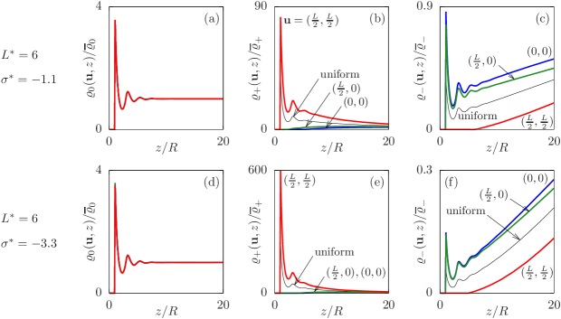
Figure 3: The plots show the number density profiles $\varrho_{i}(\mathbf{u},z)$ of the solvent ($i=0$) (see the panels (a) and (d)), of the cations ($i=+$) (see the panels (b) and (e)), and of the anions ($i=-$) (see the panels (c) and (f)) close to a planar, non-uniformly charged substrate corresponding to Fig. 2 with periodicity $L^{*}=\kappa L=6$ and mean surface charge $\displaystyle\sigma^{*}=\frac{\sigma^{(1)}}{e\kappa^{2}}=-1.1$ (see the panels (a)–(c)) and $-3.3$ (see the panels (d)–(f)). The number density profiles $\varrho_{i}(\mathbf{u},z)$ are given as functions of the normal coordinate $z>0$ for three representative lateral positions in the lateral elementary cell $[0,L)\times[L,0)$ (see Fig. 2): at the origin $\mathbf{u}=(0,0)$ (blue curves corresponding to the blue diamond), close to an edge $\mathbf{u}=(L/2,0)$ (green curves corresponding to the green triangle), and at the center point $(L/2,L/2)$ (red curves corresponding to the white dot). For comparison the number density profiles $\varrho_{i}^{(1)}(z)$ for a uniform charge distribution with surface charge density $\sigma^{(1)}$ is shown (thin black curves). For $z\to\infty$ all profiles approach the corresponding bulk number densities $\overline{\varrho}_{i}$. Close to the substrate the typical layering due to the hard cores of the fluid particles is clearly visible. Whereas the solvent number density $\varrho_{0}(\mathbf{u},z)$ (see panels (a) and (d)) varies barely as function of the lateral position $\mathbf{u}$ or the surface charge $\sigma^{*}$, the cation number density $\varrho_{+}(\mathbf{u},z)$ (see panels (b) and (e)) and the anion number densities $\varrho_{-}(\mathbf{u},z)$ (see panels (c) and (f)) are sensitive to both $\mathbf{u}$ and $\sigma^{*}$. Note that the surface charge is negative here, i.e., $\sigma^{*}<0$, so that the cations accumulate at and the anions are depleted from lateral positions close to the charged square patches of the substrate (see Fig. 2).

Figure 3 displays the number density profiles $\rho_{i}(\mathbf{u},z),i\in\{0,+,-\}$, as functions of the normal coordinate $z>0$ for three characteristic lateral positions $\mathbf{u}=(x,y)=(0,0)$ (blue curves, blue diamond in Fig. 2), $(L/2,0)$ (green curves, green triangle in Fig. 2), and $(L/2,L/2)$ (red curves, white dot in Fig. 2) at a corner, at an edge, and at the center of the lateral elementary cell $[0,L)\times[0,L)\subseteq\mathbb{R}^{2}$, respectively, for $L^{*}=6$. Panels (a)–(c) show the case $\sigma^{*}=-1.1$ whereas panels (d)–(f) show the case $\sigma^{*}=-3.3$. For comparison the corresponding profiles $\varrho_{i}^{(1)}(z)$ close to a uniformly charged substrate are depicted (see the thin black curves). It can be observed that the solvent number density profiles $\varrho_{0}(\mathbf{u},z)$ (see Figs. 3(a) and (d)) are largely insensitive to the lateral position $\mathbf{u}$ and to the magnitude of the surface charge density $|\sigma^{*}|$, because the solvent particles in the present model are electrically neutral and non-polar. Within a model for a polar solvent one can expect variations of $\varrho_{0}(\mathbf{u},z)$ to occur upon changing $\mathbf{u}$ or $\sigma^{*}$.

As the surface charge is negative, the cation number densities $\varrho_{+}(\mathbf{u},z)$ close to the substrate surface are larger than in the bulk, whereas the anion number density profiles $\varrho_{-}(\mathbf{u},z)$ close to the substrate are smaller than in the bulk. As expected, these trends are particularly pronounced for highly charged surfaces, i.e., large values of $|\sigma^{*}|$, and at lateral positions $\mathbf{u}$ corresponding to highly charged regions on the substrate.

According to Eq. (14) the lateral structure, expressed in terms of $\Delta\widehat{\varrho}_{i}(\mathbf{q},z)$, is determined by the electrostatic potential, represented by $\Delta\widehat{\psi}(\mathbf{q},z)$, as well as by the hard-core interaction, given by the third expression in Eq. (14). Upon ignoring the hard-core contribution one obtains approximate lateral number density variations

$$\Delta\widehat{\varrho}_{i}(\mathbf{q},z)\approx\Delta\widehat{\varrho}_{i}^{\text{DH}}(\mathbf{q},z):=-\beta eZ_{i}\varrho_{i}^{(1)}(z)\Delta\widehat{\psi}(\mathbf{q},z),$$ (29)

which resemble those within linear Poisson-Boltzmann (i.e., Debye-Hückel) theory. Inverse Fourier transformation leads to

$$\Delta\varrho_{i}^{\text{DH}}(\mathbf{u},z)=-\beta eZ_{i}\varrho_{i}^{(1)}(z)\Delta\psi(\mathbf{u},z)$$ (30)

so that

$$\varrho_{i}^{\text{DH}}(\mathbf{u},z):= \ \varrho_{i}^{(1)}(z)+\Delta\varrho_{i}^{\text{DH}}(\mathbf{u},z)$$

$$= \ \varrho_{i}^{(1)}(z)\left(1-\beta eZ_{i}\Delta\psi(\mathbf{u},z)\right).$$ (31)

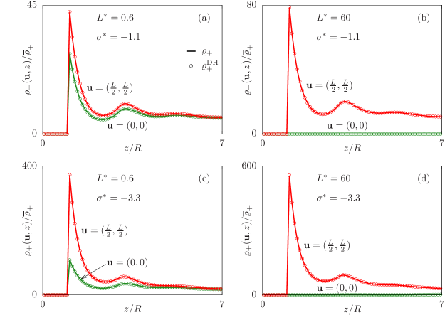
Figure 4: In order to assess the approximation $\varrho_{i}(\mathbf{r})\approx\varrho_{i}^{\text{DH}}(\mathbf{r})$ for the full number density profiles $\varrho_{i}(\mathbf{r})$ (solid curves) by the Debye-Hückel profiles $\varrho_{i}^{\text{DH}}(\mathbf{r})$ (circles) as defined in Eq. (31), the cation profiles ($i=+$) are shown for the two values $L^{*}=0.6$ (see panels (a) and (c)) and $L^{*}=60$ (see panels (b) and (d)), the two values $\sigma^{*}=-1.1$ (see panels (a) and (b)) and $\sigma^{*}=-3.3$ (see panels (c) and (d)), as well as for two lateral positions $\mathbf{u}=(0,0)$ (green curves) and $(L/2,L/2)$ (red curves). We find excellent quantitative agreement. For the large length $L^{*}=60$ the number densities $\varrho_{+}(\mathbf{u},z)$ are close to the bulk number density $\overline{\varrho}_{+}$ at the lateral position $\mathbf{u}=(0,0)$, where the substrate is uncharged within a radius of a few Debye lengths (see the green curves and circles in panels (b) and (d)).

Figure 4 compares the full number density profiles $\varrho_{i}(\mathbf{u},z)$ (solid curves) with the corresponding Debye-Hückel approximations $\varrho_{i}^{\text{DH}}(\mathbf{u},z)$ (circles) according to Eq. (31) at the lateral positions $\mathbf{u}=(0,0)$, i.e., at the origin (in green), and at $\mathbf{u}=(L/2,L/2)$, i.e., in the center of the elementary cell (in red), for lateral length scales $L^{*}\in\{0.6,60\}$, and surface charges $\sigma^{*}\in\{-1.1,-3.3\}$. It turns out, that the approximation $\varrho_{i}(\mathbf{r})\approx\varrho_{i}^{\text{DH}}(\mathbf{r})$ is reliable to a high degree, i.e., the hard-core contribution as the last term in Eq. (14) can be safely ignored. Whereas the hard-core interaction plays an important role for the number density profiles $\varrho_{i}^{(1)}(z)$ close to laterally uniformly charged substrates, it does not influence the lateral structure formation significantly.

Since the hard-core contribution as the last term in Eq. (14) is quantitatively negligible, one ends up with the approximation

$$\Delta\widehat{Q}(\mathbf{q},z)\approx \ e\sum_{i}Z_{i}\left(-\beta eZ_{i}\varrho^{(1)}_{i}(z)\right)\Delta\widehat{\psi}(\mathbf{q},z)$$

$$= \ -\beta e^{2}\sum_{i}Z_{i}^{2}\varrho^{(1)}_{i}(z)\Delta\widehat{\psi}(\mathbf{q},z)$$

$$= \ -\beta e^{2}\left(\varrho^{(1)}_{+}(z)+\varrho^{(1)}_{-}(z)\right)\Delta\widehat{\psi}(\mathbf{q},z)$$ (32)

which is equally valid.

Upon inserting Eq. (32) into the Helmholtz equation for $z>0$ (see Eq. (16)) one obtains

$$\frac{\partial^{2}\Delta\widehat{\psi}}{\partial z^{2}}(\mathbf{q},z)=\left(|\mathbf{q}|^{2}+\widetilde{\kappa}(z)^{2}\right)\Delta\widehat{\psi}(\mathbf{q},z)$$ (33)

with the abbreviation

$$\widetilde{\kappa}(z):=\sqrt{4\pi\ell_{B}\left(\varrho^{(1)}_{+}(z)+\varrho^{(1)}_{-}(z)\right)}.$$ (34)

For $z\to\infty$ the quantity $\widetilde{\kappa}(z)$ approaches the inverse Debye length, i.e., $\widetilde{\kappa}(z)\to\kappa$, as in this limit $\varrho_{\pm}^{(1)}(z)\to I$. Figure 5 shows, that $\widetilde{\kappa}(z)/\kappa$ attains its bulk value $1$ already a few particle radii $R$ away from the substrate.

Hence beyond a few particle radii $R$ away from the substrate, i.e., at $z\gg R$, Eq. (33) reduces to

$$\frac{\partial^{2}\Delta\widehat{\psi}}{\partial z^{2}}(\mathbf{q},z)\simeq\left(|\mathbf{q}|^{2}+\kappa^{2}\right)\Delta\widehat{\psi}(\mathbf{q},z),$$ (35)

with the solution

$$\Delta\widehat{\psi}(\mathbf{q},z)\propto\exp\left(-\frac{z}{\lambda(|\mathbf{q}|)}\right),\qquad\text{$z\gg R$,}$$ (36)

with the normal decay length

$$\lambda(q):=\frac{1}{\sqrt{q^{2}+\kappa^{2}}}.$$ (37)

According to Eq. (29), in the range $z\gg R$ the modes of the lateral structure $\Delta\widehat{\varrho}_{i}(\mathbf{q},z)$ decay on the same normal length scale $\lambda(|\mathbf{q}|)$. Whereas the decay length $\lambda(q)$ is a bulk quantity, the proportionality prefactor of the asymptotics in Eq. (36) dependson the surface charge density (see Eq. (21)) as well as on details of the ion number density profiles $\varrho^{(1)}_{+}(z)$ and $\varrho^{(1)}_{-}(z)$ (see Eqs. (33) and (34)).

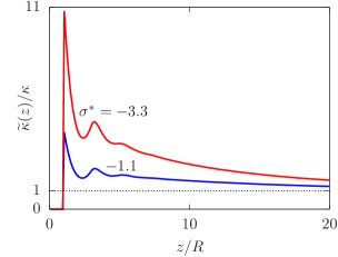
Figure 5: For $z\to\infty$ the function $\widetilde{\kappa}(z)$, defined in Eq. (34), approaches the inverse Debye length $\kappa$. Beyond the hard-core layering range, $\widetilde{\kappa}(z)/\kappa$ attains unity within a few particle radii $R$.

III.2 Lateral profiles

The length scale, on which the lateral modes $\mathbf{q}$ decay in the normal direction, is given by $\lambda(|\mathbf{q}|)$ (see Eq. (37)). It attains its maximum value $\kappa^{-1}$, i.e., the Debye length, at $\mathbf{q}=0$. Accordingly, the normal decay length $\lambda(|\mathbf{q}|)$ is not larger than the Debye length $\kappa^{-1}$. Upon increasing $|\mathbf{q}|$ the normal decay length $\lambda(|\mathbf{q}|)$ decreases monotonically.

Since $\sigma^{(1)}=\widehat{\sigma}_{00}$ and

$$\Delta\sigma(\mathbf{u}=(x,y))=\sigma(\mathbf{u})-\sigma^{(1)}=$$

$$\sum_{\begin{smallmatrix}k,\ell\in\mathbb{Z}\\ (k,\ell)\not=(0,0)\end{smallmatrix}}\widehat{\sigma}_{k\ell}\ \exp\left(\frac{2\pi i}{L}(kx+\ell y)\right),$$ (38)

i.e., $\Delta\widehat{\sigma}(\mathbf{q}=\mathbf{q}_{00}=0)=0$ due to Eq. (23), the smallest wave number $\displaystyle|\mathbf{q}|=|\mathbf{q}_{k\ell}|=\frac{2\pi}{L}\sqrt{k^{2}+\ell^{2}}$ contributing to a lateral structure is $\displaystyle q_{\text{min}}=|\mathbf{q}_{\pm 1,0}|=|\mathbf{q}_{0,\pm 1}|=\frac{2\pi}{L}$. Hence the lateral structure induced by a non-uniformly charged substrate decays in normal direction on the length scale

$$\lambda_{\text{max}} =\lambda(q_{\text{min}})=\frac{1}{\displaystyle\sqrt{\left(\frac{2\pi}{L}\right)^{2}+\kappa^{2}}}=\frac{L}{\sqrt{(2\pi)^{2}+(L^{*})^{2}}}$$

$$\simeq\begin{cases}\displaystyle\frac{L}{2\pi},&\text{for $L^{*}\ll 2\pi$}\\[7.0pt] \kappa^{-1},&\text{for $L^{*}\gg 2\pi$.}\end{cases}$$ (39)

Figure 6 displays the dependence of $\lambda_{\text{max}}$ on the length scale parameter $L^{*}=\kappa L$. At short length scales $L^{*}\ll 2\pi$ a linear dependence is found, which crosses over to $\lambda_{\text{max}}\simeq\kappa^{-1}$ (Debye length) at large length scales $L^{*}\gg 2\pi$.

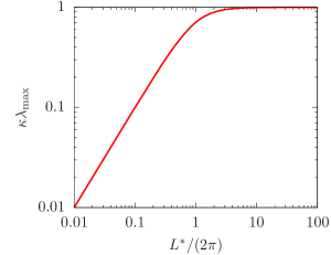
Figure 6: At $L^{*}=\kappa L\approx 2\pi$ the largest normal decay length $\lambda_{\text{max}}$ of the laterally non-uniform modes (see Eq. (39)) crosses over from a linear regime at short length scales $L^{*}\ll 2\pi$ to $\lambda_{\text{max}}\simeq\kappa^{-1}$ (i.e., the Debye length) at large length scales $L^{*}\gg 2\pi$.

From the quantitatively reliable approximation $\varrho_{i}(\mathbf{r})\approx\varrho^{\text{DH}}_{i}(\mathbf{r})$ (see the previous Subsec. III.1 and in particular Fig. 4) one can infer that the lateral structure of the electrolyte solution, i.e., $\varrho_{i}(\mathbf{r})$, is determined by the lateral structure of the electrostatic potential $\psi(\mathbf{r})$ (see Eq. (31)). Accordingly, Fig. 7 displays two sequences of lateral profiles of the electrostatic potential $\psi(\mathbf{u},z)$, i.e., functions of $\mathbf{u}$ with $z$ fixed, at the normal positions $z=0$, $R$, $\lambda_{\text{max}}$, and $2\lambda_{\text{max}}$ for $L^{*}=0.6$ (left column: (a), (c), (e), (g)) and $60$ (right column: (b), (d), (f), (h)). Qualitatively, the difference of the electrostatic potential between lateral positions associated with large and with small surface charge densities diminishes with increasing distance from the substrate. However, although the normal decay length $\lambda_{\text{max}}$ is very different for the two cases ($\kappa\lambda_{\text{max}}\approx 0.1$ for $L^{*}=0.6$ and $\kappa\lambda_{\text{max}}\approx 1$ for $L^{*}=60$), the decay of the lateral structure of the two as function of $z/\lambda_{\text{max}}$ is similar.

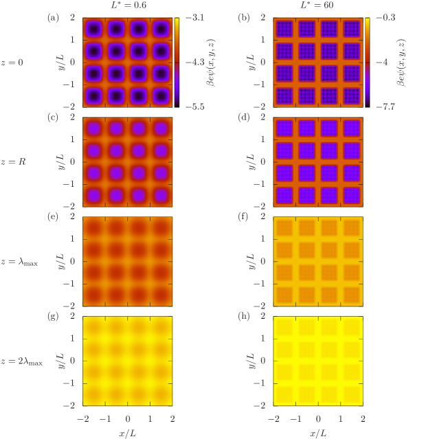
Figure 7: The reduced electrostatic potential $\beta e\psi(\mathbf{u},z)$ as function of the lateral position $\mathbf{u}$ for fixed distances $z\geq 0$ from the substrate determines, and hence represents, the lateral structure of the electrolyte solution (see Eq. (31)). The left column corresponds to the case $L^{*}=0.6$ (short lateral length scale) and the right column to the case $L^{*}=60$ (large lateral length scale). For each case, the lateral structure decays in normal direction on the length scale of $\lambda_{\text{max}}$ (see Eq. (39)). The contrast between charged and neutral parts of the substrate at $z=0$ is clearly visible (see panels (a) and (b)). In the first contact layer of the fluid at $z=R$ (see panels (c) and (d)), the contrast is still present, but slightly blurred. At the distance $z=\lambda_{\text{max}}$ (see panels (e) and (f)) the contrast is diminished substantially and even more so at $z=2\lambda_{\text{max}}$ (see panels (g) and (h)). The decay of the lateral structure as function of $z/\lambda_{\text{max}}$ is similar, irrespective of the lateral length scale $L^{*}$. Upon increasing $z$, for $L^{*}=0.6$ the rectangular shape of the charged pattern is washed out in favor of circular patterns. For $L^{*}=60$ the rectangular shape of the patterns remains even for $z=2\lambda_{\text{max}}$.

III.3 Interfacial tension

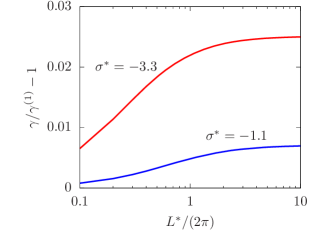
Figure 8: Upon increasing the lateral length scale $L^{*}$ the interfacial tension $\gamma$ increases with respect to its value $\gamma^{(1)}$ of a uniformly charged substrate. In sync with the behavior of the normal decay length $\lambda_{\text{max}}$ (see Eq. (39) and Fig. 6), the interfacial tension $\gamma$ levels off for $L^{*}\gg 2\pi$.

The findings discussed so far lead to the picture of a surface layer of thickness $\lambda_{\text{max}}$ in which a non-uniform surface charge density, characterized by a lateral length scale $L$, can be sensed by the electrolyte solution. This thickness $\lambda_{\text{max}}$ is found to increase as function of $L$ as long as $L^{*}=\kappa L\ll 2\pi$, whereas it is approximately constant for $L^{*}\gg 2\pi$. Therefore, one can expect that the interfacial tension $\gamma$ (see Subsec. II.4) exhibits the same trend. This is indeed the case, as it is shown in Fig. 8 for the surface charges $\sigma^{*}=-3.3$ (red curve) and $-1.1$ (blue curve). However, the interfacial tension $\gamma$ of a non-uniformly charged substrate turns out to be limited to at most a few percent above the interfacial tension $\gamma^{(1)}$ of a uniformly charged substrate with the same mean surface charge density.

IV Summary, conclusions, and Outlook

The present investigation is devoted to the structure formation in a dilute electrolyte solution close to a non-uniformly charged planar substrate (see Fig. 1). In dilute electrolyte solutions the Debye screening length $\kappa^{-1}$ is substantially larger than the size of the fluid molecules $R$ so that, in principle, the spatial region of according thickness $\kappa^{-1}$ close to a charged substrate can be sensitive to the surface charge distribution. However, the lateral length scale $L$ of the charge distribution on the substrate turns out to play a role, too. In the present study periodic charge distributions with periodicity $L$ of arbitrary magnitude are considered (see Fig. 2), and the corresponding laterally non-uniform number density profiles of the fluid particles are calculated via expansion about the profiles of a uniform substrate with the same mean surface charge density (see Fig. 3). It is found that the lateral structure is mainly determined by the electrostatic potential, i.e., not by molecular-ranged forces like the hard-core interaction, so that the laterally non-uniform contributions of the number density profiles can be accurately approximated by a Debye-Hückel-like expression (see Eq. (31)), disregarding hard-core contributions (see Fig. 4). As a consequence, for normal distances not too close to the substrate, i.e., at $z$-coordinates with $\widetilde{\kappa}(z)/\kappa$ in Fig. 5 close to unity, the lateral contributions of the electrostatic potential, and hence of the number densities, decay on the scale $\lambda_{\text{max}}$ given in Eq. (39) (see Fig. 6). For lateral length scales $L$ with $L^{*}=\kappa L\ll 2\pi$, the normal decay length is varying with $L$ according to $\lambda_{\text{max}}\approx L/(2\pi)$, whereas for $L^{*}\gg 2\pi$ it levels off at the value of the Debye length, $\lambda_{\text{max}}\approx\kappa^{-1}$. As shorter length scales $L^{*}\ll 2\pi$ decay more rapidly than larger ones, a washing out of fine details at increasing distance from the surface occurs (see Fig. 7). Ultimately only structures at length scales $L^{*}\gg 2\pi$ contribute to the lateral structure. In terms of the interfacial tension of the non-uniformly charged substrate an increase with $L$ is observed for $L^{*}\ll 2\pi$ which saturates for $L^{*}\gg 2\pi$ (see Fig. 8).

Equation (36) in conjunction with Eq. (31) states, that at distances $z\gg\lambda(q)$ (see Eq. (37)) details of a surface charge distribution with wave number $q=|\mathbf{q}|$ become irrelevant for the lateral structure of an adjacent electrolyte solution. Hence, at larger distances from the substrate, only less fine details of a surface charge distribution can be resolved. Ultimately, at distances $z\gtrsim\kappa^{-1}$ details with wave numbers $q=|\mathbf{q}|\gtrsim\kappa$, i.e. with lateral length scales $L\lesssim 2\pi\kappa^{-1}$, are washed out so that only surface structures with lateral length scales $L\gtrsim 2\pi\kappa^{-1}$ matter. The strength of the influence of these large-scale structures decay exponentially with a decay length given by the Debye screening length $\kappa^{-1}$. Therefore, when modeling electrolyte solutions with molecular length scale $R$, one can safely ignore surface non-uniformities at length scales $L\lesssim 2\pi R$, which, for molecular fluids, can be close to a nanometer. Finally, the present study shows that macroscopic descriptions of electrolyte solutions, i.e., on length scales larger than the Debye length $\kappa^{-1}$, are carried out consistently by considering surface details on lateral length scales larger than $2\pi\kappa^{-1}$ only.

Two main conclusions can be drawn from the present study: (i) Microscopic hard-core interactions have negligible influence on the lateral structure formation of electrolyte solutions close to non-uniformly charged substrates. (ii) Fine details of lateral non-uniformities have negligible influence beyond a certain (short) distance from the substrate. Accordingly, the approach of disregarding the size of molecules and treating them as point particles (see many previous theoretical studies concerning the interaction between non-uniformly charged colloidal particles) can be justified or readily adjusted. Generally, the present study shows that on macroscopic length scales only macroscopically large features of the surface structure are visible. This allows for local descriptions of fluids in terms of partial differential equations, e.g., the Young-Laplace equation in hydrostatics. The dominant correlation length of a fluid, which for a dilute electrolyte solution of a non-critical solvent is the Debye length, separates length scales into macroscopic and microscopic ones. From a microscopic point of view, there is a smooth crossover of the fluid structure from small to large length scales, whereas microsopic details can be safely ignored from a macroscopic point of view.

Several directions of applications of the gained insight are conceivable: The presented approach, i.e., to consider deviations from laterally uniform reference density profiles and to ignore hard-core interactions, could be exploited in various numerical analyses of fluid structures, including computer simulations. This way studies of large laterally non-uniform systems could become feasible. Furthermore, given a certain length scale, the above insight is useful in order to distinguish relevant from irrelevant surface details. This is of importance not only for theoretical considerations or numerical applications, but also for efficiently solving practical problems, such as guiding flows in nanochannels, patterning surface structures of catalytic reactors, or designing electrochemical devices. Finally, a common understanding of the small effect microscopic features have on macroscopic length scales (and vice versa) could be helpful for the scientific discourse by avoiding confusion when comparing experimental or theoretical results obtained within methods the spatial resolution of which are associated with incompatible length scales.

References

- (1) J.W. Gibbs, The scientific papers, Vol. 1 (Longmans, London, 1961).
- (2) H. Helmholtz, Studien über electrische Grenzschichten, Ann. Phys. Chem. 7, 337 (1879).
- (3) M. Gouy, Sur la constitution de la charge électrique à la surface d’un électrolyte, C.R. Acad. Sci. 149, 654 (1909).
- (4) M. Gouy, Sur la constitution de la charge électrique à la surface d’un électrolyte, J. Physique 9, 457 (1910).
- (5) D.L. Chapman, A Contribution to the Theory of Electrocapillarity, Philos. Mag. 25, 475 (1913).
- (6) D.C. Grahame, The electrical double layer and the theory of electrocapillarity, Chem. Rev. 41, 441 (1947).
- (7) P. Richmond, Electrical Forces between Particles with Arbitrary Fixed Surfce Charge Distributions in Ionic Solution, J. Chem. Soc.: Faraday Trans. 2 70, 1066 (1974).
- (8) P. Richmond, Electrical Forces between Particles with Discrete Periodic Surface Charge Distributions in Ionic Solution, J. Chem. Soc.: Faraday Trans. 2 70, 1154 (1975).
- (9) P. Debye and E. Hückel, Zur Theorie der Elektrolyte, Phys. Z. 24, 185 (1923).
- (10) W.B. Russel, D.A. Saville, and W.R. Schowalter, Colloidal Dispersions (Cambridge University Press, Cambridge, 1989).
- (11) D.A. McQuarrie, Statistical mechanics (Universal Science Books, Sausalito, 2000).
- (12) R.J. Hunter, Foundations of Colloid Science (Oxford University Press, Oxford, 2001).
- (13) D. Ben-Yaakov, D. Andelman, and H. Diamant, Interaction between heterogeneously charged surfaces: surface patches and charge modulation, Phys. Rev. E 87, 022402 (2013).
- (14) S. Ghosal and J.D. Sherwood, Screened Coulomb interactions with non-uniform surface charge, Proc. R. Soc. A 473, 20160906 (2017).
- (15) M. Mußotter, M. Bier, and S. Dietrich, Electrolyte solutions at heterogeneously charged substrates, Soft Matter 14, 4126 (2018).
- (16) J.D. Sherwood and S. Ghosal, Effect of Nonzero Solid Permittivity on the Electrical Repulsion between Charged Surfaces, Langmuir 36, 2592 (2020).
- (17) R.M. Adar and D. Andelman, Electrostatic attraction between overall neutral surfaces, Phys. Rev. E 94, 022803 (2016).
- (18) R.M. Adar and D. Andelman, Osmotic pressure between arbitrarily charged surfaces: a revisited approach, Eur. Phys. J. E 41, 11 (2018).
- (19) A. Naji, D.S. Dean, J. Sarabadani, R.R. Horgan, and R. Podgornik, Fluctuation-induced interaction between randomly charged dielectrics, Phys. Rev. Lett. 104, 060601 (2010).
- (20) A. Naji, M. Ghodrat, H. Komaie-Moghaddam, and R. Podgornik, Asymmetric Coulomb fluids at randomly charged dielectric interfaces: anti-fragility, overcharging and charge inversion, J. Chem. Phys. 141, 174704 (2014).
- (21) M. Ghodrat, A. Naji, H. Komale-Moghaddam, and R. Podgornik, Ion-mediated interactions between net-neutral slabs: weak and strong disorder effects, J. Chem. Phys. 143, 234701 (2015).
- (22) M. Ghodrat, A. Naji, H. Komaie-Moghaddama, and R. Podgornik, Strong coupling electrostatics for randomly charged surfaces: antifragility and effective interactions, Soft Matter 11, 3441 (2015).
- (23) A. Naji,K. Hejazi, E. Mahgerefteh, and R. Podgornik, Charged nanorods at heterogeneously charged surfaces, J. Chem. Phys. 149, 134702 (2018).
- (24) R.M. Adar, D. Andelman, and H. Diamant, Electrostatics of patchy surfaces, Adv. Colloid Interface Sci. 247, 198 (2017).
- (25) A. Bakhshandeh, A.P. dos Santos, A. Diehl, and Y. Levin, Interaction between random heterogeneously charged surfaces in an electrolyte solution, J. Chem. Phys. 142, 194707 (2015).
- (26) S. Zhou, Effective electrostatic interactions between two overall neutral surfaces with quenched charge heterogeneity over atomic length scale, J. Stat. Phys. 169, 1019 (2017).
- (27) C. McCallum, S. Pennathur, and D. Gillespie, Two-Dimensional electric double layer structure with heterogeneous surface charge, Langmuir 33, 5642 (2017).
- (28) M. Mußotter, M. Bier, and S. Dietrich, Heterogeneous surface charge confining an electrolyte solution, J. Chem. Phys. 152, 234703 (2020).
- (29) R. Evans, The nature of the liquid-vapour interface and other topics in the statistical mechanics of non-uniform, classical fluids, Adv. Phys. 28, 143 (1979).
- (30) R. Evans, Microscopic theories of simple fluids and their interfaces, in Les Houches, Session XLVIII, 1988 — Liquides aux interfaces / Liquids at interfaces, edited by J. Charvolin, J.F. Joanny, and J. Zinn-Justin (North-Holland, Amsterdam, 1990), p. 1.
- (31) R. Evans, Density functionals in the theory of nonuniform fluids, in Fundamentals of inhomogeneous fluids, edited by D. Henderson (Marcel Dekker, New York, 1992), p. 85.
- (32) R. Roth, R. Evans, A. Lang, and G. Kahl, Fundamental measure theory for hard-sphere mixtures revisited: The white bear version, J. Phys.: Condens. Matter 14, 12063 (2002).
- (33) J.L. Lebowitz and E.H. Lieb, Existence of Thermodynamics for Real Matter with Coulomb Forces, Phys. Rev. Lett. 22, 631 (1969).
- (34) L. Bocquet, E. Trizac and M. Aubouy, Effective charge saturation in colloidal suspensions, J. Chem. Phys. 117, 8138 (2002).