OOD-Probe: A Neural Interpretation of Out-of-Domain Generalization

Abstract

The ability to generalize out-of-domain (OOD) is an important goal for deep neural network development, and researchers have proposed many high-performing OOD generalization methods from various foundations. While many OOD algorithms perform well in various scenarios, these systems are evaluated as “black-boxes”. Instead, we propose a flexible framework that evaluates OOD systems with finer granularity using a probing module that predicts the originating domain from intermediate representations. We find that representations always encode some information about the domain. While the layerwise encoding patterns remain largely stable across different OOD algorithms, they vary across the datasets. For example, the information about rotation (on RotatedMNIST) is the most visible on the lower layers, while the information about style (on VLCS and PACS) is the most visible on the middle layers. In addition, the high probing results correlate to the domain generalization performances, leading to further directions in developing OOD generalization systems.

1 Introduction

Out-of-domain (OOD) generalization is an essential goal in developing deep neural network systems. Most existing approaches to developing OOD-generalizable systems follow the invariance principle (Arjovsky et al., 2020), stating that the data representation should allow the optimal predictor performance to match across environments. Two avenues of work stem from this invariance principle. The first avenue focuses on learning a data representation that remains invariant across environments. This goal can translate to regularization terms that minimize the discrepancy across environments (Li et al., 2018a), or auxiliary learning objectives encouraging the representations to be indistinguishable (Ganin et al., 2015; Li et al., 2018b). The second avenue focuses on letting the optimal predictor performance match across environments. To align the predictors, we can align the gradients (Shahtalebi et al., 2021; Shi et al., 2021; Koyama & Yamaguchi, 2021; Parascandolo et al., 2020) or prevent the predictors to become overly confident (Pezeshki et al., 2021; Wald et al., 2021). This avenue requires a diverse collection of environments, which can be implemented by perturbing the domains by group (Sagawa* et al., 2020), data samples (Krueger et al., 2021; Yan et al., 2020), features (Huang et al., 2020), or some combinations thereof (Huang et al., 2022).

Each paper proposes some improvements against multiple previous algorithms and verifies by evaluating accuracy-based scores in novel domains, including the worst group and leave-one-domain-out accuracy (Gulrajani & Lopez-Paz, 2020; Ye et al., 2021; Hendrycks et al., 2021). While these evaluation protocols provide a holistic perspective for the performance of the networks, they do not reveal the intrinsic mechanisms of generalization. Many questions remain unanswered, including:

1. Do the neural networks arrive at invariant representations somewhere in the network? If yes, where?

2. Do the OOD generalization algorithms encourage the neural networks to learn generalizable representations? If yes, how well do these representations generalize?

We argue that, to answer these questions, we should inspect the intermediate representations of the deep neural networks. To attempt answers, we resort to a tool widely used in the interpretable AI literature – probing. After the deep neural networks are trained, a diagnostic classifier (“probe”) is trained to predict a target from the intermediate representations. A higher probing performance indicates the representation is more relevant to the target (Alain & Bengio, 2017). Probing analysis reveals many aspects about the intrinsics of deep neural networks (primarily language models), including the encoded semantic knowledge (Pavlick, 2022) and linguistic structures (Rogers et al., 2020; Manning et al., 2020). For example, Tenney et al. (2019) found that BERT (Devlin et al., 2019), a Transformer-based language model, automatically forms a pipeline to process textual data in a way that resembles traditional NLP pipelines. The probing results, together with some co-occurrence statistics, can predict the extent to which a feature influences the model’s predictions (Lovering et al., 2021). Probing has demonstrated strong potential for examining the intrinsic mechanisms of deep neural networks.

To answer Q1 and Q2, we set up a framework, OOD-Probe, that attaches an auxiliary probing module to the deep neural network models. OOD-Probe predicts the domain attribute from the intermediate representations.

We apply OOD-Probe to 22 algorithms in DomainBed (Gulrajani & Lopez-Paz, 2020). Overall, the neural networks do not arrive at truly invariant representations. In addition, the probing results reveal interesting patterns that persist across algorithms and differ across datasets. On RotatedMNIST (Ghifary et al., 2015), the lower layers show easier-to-decode domain attributes. On VLCS (Fang et al., 2013) and PACS (Li et al., 2017a), the middle layers show the most easily decodable domain attribute. The higher probing performances also correlate well to the OOD generalization performances. In aggregate, probing performance is predictive of domain generalization performance and provides evaluations in finer granularity. We call for further attention to the models’ intrinsics and discuss how probing can help develop OOD generalization systems. Our analysis codes will be released at anonymized-url.

2 Method

2.1 Problem setting

We want to set up a neural network system that learns a mapping $f:x\in\mathcal{X}_{e}\rightarrow y\in\mathcal{Y}_{e}$, for $e\in\mathcal{E}$. In the “leave-one-domain-out” setting of OOD generalization problem, the system $f$ is trained on $M$ training environments $\mathcal{E}_{tr}=\{e_{1},e_{2},...,e_{M}\}$ and tested on a novel environment $e_{M+1}$.

The neural network $f$ learns a representation $\Phi$ to represent the random variable $X$ and preserve rich information about $Y$. Usually, the neural networks contain a Featurizer (e.g., ResNet (He et al., 2016) or multilayer CNNs) and a Classifier (e.g., Linear), as shown in Figure 1. Both types of Featurizer contain multiple intermediate representations. For multilayer CNNs, we probe the representation for each layer. For ResNet, since the residual connections within each block accelerates the passage of information, we probe the representation from each block.

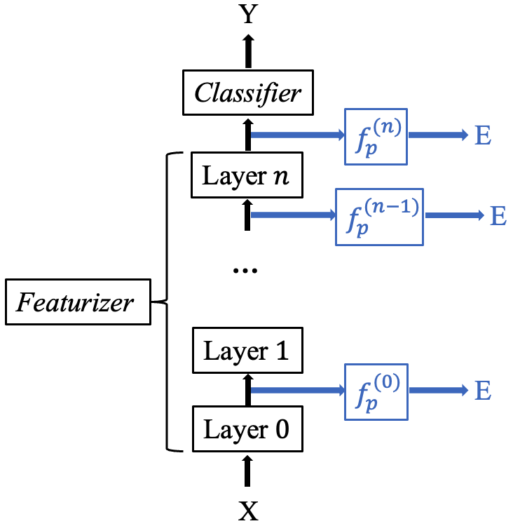
Figure 1: A schematic diagram of the proposed framework. The blue parts constitute of the probing module.

2.2 Probing module

The key component in our neural explanation framework is a probing module, which consists of one or more probes. For a representation $\Phi$ of a trained neural network, we attach a probe, which is a post-hoc classifier that predicts a predefined target: $f_{p}:\Phi\rightarrow T$, where the choice of $T$ depends on the (e.g., linguistic) aspect of the representations to be examined (Ettinger et al., 2018; Conneau & Kiela, 2018). We set the target $T$ as the environment label $E$. Without loss of generality, one can designate alternative targets as the probing target.

Explaining OOD with probing accuracy

Many other chocies of $\textrm{Perf}(f_{p})$ have been discussed in the probing literature, including the minimum description length of an imaginary channel that transmits information from $\Phi$ to $E$ (Voita & Titov, 2020), or some variants of $\Phi-E$ mutual information (Pimentel et al., 2020; Hou & Sachan, 2021; Hewitt et al., 2021). These can be approximated by combinations of cross-entropy losses of probing classifiers. Practically, the precise estimation of information-theoretic terms involving high-dimensional random variables (e.g., $\Phi$) is extremely hard due to limitations of existing estimators (McAllester & Stratos, 2020; Song & Ermon, 2019). Accuracy is still the most popular choice of $\textrm{Perf}(f_{p})$ for classification-type probing problems (Belinkov, 2021; Ravichander et al., 2021; Conneau et al., 2018). In this paper, we also use accuracy. This widely used $\textrm{Perf}(f_{p})$ score allows for comparison to the performances of OOD generalization algorithms – we elaborate the analyses in Section 4.

3 Experimental setup

3.1 Data

We use four datasets that are widely used in the OOD generalization literature: RotatedMNIST (Ghifary et al., 2015), ColoredMNIST (Arjovsky et al., 2020), VLCS (Fang et al., 2013), and PACS (Li et al., 2017a). These datasets specify classification problems in multiple domains. The variable that denotes the domain, $E$, affects the joint distributions $P(X,Y)$ in distinct manners.

In RotatedMNIST, $E$ specifies the degree of rotation of the handwritten digits. The $E$ in ColoredMNIST corresponds to the proportion of images assigned a colour (red or green). The $f_{p}:\Phi\rightarrow E$ probing classification performances would be low if the model relies on the digits’ shapes but not other factors (e.g., the rotated angle and the colours).

In PACS, $E$ specifies four distinct styles of images – photo, art painting, cartoon, and sketch – all containing images belonging to seven classes: dog, elephant, giraffe, guitar, horse, house, and person. $E$ in VLCS specifies the originating dataset, all of which contain images belonging to five common categories: bird, cat, chair, dog, person. In both PACS and VLCS, the $f_{p}:\Phi\rightarrow E$ probing classification performance would be low if the representation describes the content but not the styles of the objects.

3.2 OOD Algorithms

We attach the probing module to evaluate 22 DomainBed algorithms using their default hyperparameters. The average test-domain out-split accuracies in leave-one-domain-out evaluation are reported in Table 1.

3.3 Setting up the probing module

The most popular type of classifier in the probing literature is a fully-connected linear classifier. Compared to more complicated classifiers, linear classifiers are higher in selectivity (Hewitt & Liang, 2019), i.e., there is a more significant accuracy difference between highly informative representations and less informative ones (specified by control experiments).

Many algorithms in OOD generalization either use multilayer CNNs or ResNet as the Featurizer. The immediate input to the Classifier is a $D$-dimensional vector. All other hidden representations at layer $i$ follow the shape $(C^{(i)},H^{(i)},W^{(i)})$, where $C^{(i)}$, $H^{(i)}$, and $W^{(i)}$ are the number of channels, height, and width at the $i^{\textrm{th}}$ layer, respectively. We flatten the representations to $C^{(i)}\times H^{(i)}\times W^{(i)}$-dimensional vectors and input them to the probes.

Two types of Featurizer are used in our experiments: 4-layer CNN for RotatedMNIST and ColoredMNIST, and a ResNet-18 for VLCS and PACS. For the former, we attach a probe at the output of each Conv layer. For the latter, we attach a probe at the output of each block. For both types of networks, we add a classifier to probe the output of the Featurizer.

3.4 Probing procedure

We checkpoint the neural networks trained by OOD generalization algorithms and train the probing classifiers from the frozen checkpoints using the same train/validation splits as the OOD training. The probing also follow a “leave-one-domain-out” setting: to probe a model $f$ trained on domains $\mathcal{E}_{tr}$ (i.e., leaving out $e_{M+1}$), we train the probing classifier on the same domains to predict $1..M$.

How many data samples are enough for the probes? We used an off-the-shelf script to recommend probing dataset sizes based on the finite function space bound (Zhu et al., 2022). For the probes we set up, we need between 230k to 270k data samples to bound the uncertainty of the probing accuracy within $\pm 2\%$, and one epoch (containing $N=5,000$ batches of 64 data samples, totaling 320k data samples) suffices. As an empirical note, most probes’ validation accuracies saturate with much fewer than one epoch of samples. Figure 4 and 5 (in the Appendix) provide some examples.

4 Experiment Results

4.1 DG algorithms do not remove environment-specific information

Figure 3 shows the probing accuracy results $\textrm{Perf}(f_{p})$, averaged across all domains in the “leave-one-domain-out” setting. To interpret the accuracy results, let us first define a “dummy classifier” as one that randomly selects a label with uniform probability. On any dataset with n_class distinct labels, the dummy classifier is expected to achieve $\frac{1}{\textrm{n\_class}}$ accuracy – a dummy accuracy. While a worse accuracy is achievable, it is not a meaningful baseline. We set $\frac{1}{\textrm{n\_class}}$ to the lower bounds for the colour bars in Figure 3.

An accuracy higher than the dummy accuracy by a large margin requires much information from either the data samples or the data distributions. This is observed in all four datasets and most probing tests, indicating that OOD algorithms do not completely remove the environment-specific information. Why is this the case? Here are two alternative hypotheses:

• While the complete removal of environment-specific information is a desirable goal, the domain-invariant representations are hard to arrive at for current DNN-based learning systems.

• In addition to being invariant among environments, the representations should also be highly beneficial for the original classification problem $f:\Phi\rightarrow Y$. The multiple optimization goals define a complex game where the optimal representations themselves follow a “trade-off” among these goals.

4.2 Layerwise patterns across algorithms

Following the rows of Figure 3, consistent patterns are observable. $\textrm{Perf}(f_{p})$ decreases as we probe the upper layers for RotatedMNIST. The probing results on ColoredMNIST show a similar pattern, but this trend is not as consistent across algorithms. Note that the probing performances are only slightly above the dummy accuracy at all layers.

On VLCS and PACS, an “increase-then-decrease” pattern is visible as we probe into higher layers. The representations from the middle blocks of ResNet-18 encode the domain information in easier-to-decode manners than the remaining blocks. Note that the representation from a block, $\Phi^{(i+1)}$, is processed from the representation of the previous block, $\Phi^{(i)}$. Therefore, the data processing inequality guarantees that the information about the environment does not decrease as the block number $i$ increases, i.e., $I(\Phi^{(i)}\,;\,E)\geq I(\Phi^{(i+1)}\,;\,E)$. In other words, the ResNets do not increase the domain information – they encode the domain information more linearly in the middle parts.

Note that the algorithms with similar generalization performance $\textrm{Perf}(f_{g})$ could have markedly different probing performances $\textrm{Perf}(f_{p})$. For example, CDANN and CORAL achieve $\textrm{Perf}(f_{g})$ of 0.97 and 0.98, respectively, on RotatedMNIST. Their probing performances on lower layers are similar, but on the last hidden representation, they get $\textrm{Perf}(f_{p})^{(4)}$ of 0.55 and 0.26, respectively. When the models do not generalize, their representations might encode more or less linearly readable information about the environments.

4.3 Layerwise correlations to the OOD performance

To further understand the utility of the probing performances, we compute the Pearson correlation of $\textrm{Perf}(f_{p})$ and $\textrm{Perf}(f_{g})$. Note that the algorithms with values markedly ($\geq 3\sigma$ where $\sigma$ is the std in Table 1) different from the results report by the DomainBed paper are removed. Table 2 (in Appendix) shows the results. Additionally, Figure 2 in the Appendix shows the correlation heatmaps. The lower layers of networks on RotatedMNIST show strong correlations, indicating that a linear encoding of the rotation might be beneficial for the generalization. The linear encoding of the styles on PACS shows a similar correlation trend, as reflected by the high correlation values on probes 2 and 3. This trend is slightly different for VLCS, where the Probe_2 results, which show the highest $\textrm{Perf}(f_{p})$, do not correlate as strongly to the OOD performance.

The above correlations might be affected by some confounding factors, e.g., the inclusion of individual algorithms. To control for this factor, we also compute the correlation w.r.t each algorithm. Tables 3-6 (in Appendix) show the results. In general, $\textrm{Perf}(f_{p})$ are positively correlated to $\textrm{Perf}(f_{g})$ for RotatedMNIST, ColoredMNIST, and PACS. The correlations are mostly negative for VLCS.

5 Discussion

Setting up probing targets

The environment attribute $E$ is the most convenient target to use, but whether it is the most suitable probing target to set up remains an open question. Our intuition is that a feature $T$ can be a better alternative for the environment attribute $E$ if it can specify the data shift between the environments concretely. Otherwise, one can always use the environment attribute. The interpretable NLP literature has many attempts to run carefully-controlled trials that use features to specify the difference between the environments (Warstadt & Bowman, 2020; McCoy et al., 2019; Kaushik et al., 2019). While this approach to constructing datasets is expensive, it allows the designated features to serve as informative probing targets.

Fine-grained evaluations for generalization

The findings from OOD-Probe open up several possibilities for improving OOD generalization using fine-grained evaluation signals, at least in the following two ways. First, since different modules in the network demonstrate different mechanisms for processing domain-related information, targeted designs may be beneficial. For example, objective functions can be set up to encourage learning linear encoding of target features in lower layers. Second, probing allows a convenient feedback “dashboard” for viewing the effects of design choices in building DNN models.

Privacy, fairness, and societal impacts

The problem of learning and evaluating high-quality representations that are invariant across domains has broad societal impacts. In privacy, the “domain attribute” can be the personal identity. This problem can translate to “removing the speaker attribute from voice while keeping the sounds recognizable” (Tomashenko et al., 2022). If the “domain attribute” refers to the demographic property, the problem can be formulated as learning a rich and fair representation (Zemel et al., 2013). The algorithms that remove protected attributes can have profound long-term impacts on multiple groups (Liu et al., 2018; Khani & Liang, 2021) – we defer to Mehrabi et al. (2022) for a summary.

6 Conclusion

While OOD generalization is an appealing goal for developing deep neural network systems, their evaluations can be more fine-grained. We propose OOD-Probe, a flexible framework that inspects the neural networks and provides layerwise scores regarding their encoding of the domain attributes. We find patterns that differ across several OOD datasets but remain relatively stable across many algorithms on DomainBed. The probing results show correlation and predictability to the generalization performance, opening up future paths in developing generalizable neural networks.

Appendix

Appendix A Experimental Results

Table 1: Domain generalization leave-one-domain-out accuracy ($\pm$ std)

Algorithm	RotatedMNIST	ColoredMNIST	VLCS	PACS
ANDMask (Parascandolo et al., 2020)	$0.96\pm 0.03$	$0.55\pm 0.30$	$0.69\pm 0.18$	$0.79\pm 0.10$
CAD (Ruan et al., 2021)	$0.97\pm 0.02$	$0.51\pm 0.33$	$0.67\pm 0.12$	$0.71\pm 0.12$
CDANN (Li et al., 2018b)	$0.97\pm 0.03$	$0.54\pm 0.30$	$0.53\pm 0.27$	$0.18\pm 0.08$
CORAL (Sun & Saenko, 2016)	$0.98\pm 0.01$	$0.51\pm 0.23$	$0.73\pm 0.16$	$0.83\pm 0.07$
CondCAD (Ruan et al., 2021)	$0.97\pm 0.02$	$0.49\pm 0.33$	$0.66\pm 0.08$	$0.77\pm 0.09$
DANN (Ganin et al., 2015)	$0.97\pm 0.03$	$0.53\pm 0.33$	$0.44\pm 0.26$	$0.21\pm 0.05$
ERM (Vapnik, 1991)	$0.98\pm 0.02$	$0.52\pm 0.25$	$0.74\pm 0.16$	$0.83\pm 0.07$
GroupDRO (Sagawa* et al., 2020)	$0.98\pm 0.02$	$0.55\pm 0.22$	$0.73\pm 0.15$	$0.83\pm 0.07$
IB_ERM (Ahuja et al., 2021)	$0.98\pm 0.01$	$0.50\pm 0.29$	$0.74\pm 0.14$	$0.79\pm 0.08$
IB_IRM (Ahuja et al., 2021)	$0.20\pm 0.07$	$0.51\pm 0.01$	$0.49\pm 0.10$	$0.13\pm 0.07$
IRM (Arjovsky et al., 2020)	$0.70\pm 0.12$	$0.56\pm 0.06$	$0.49\pm 0.10$	$0.16\pm 0.09$
MLDG (Li et al., 2017b)	$0.97\pm 0.02$	$0.52\pm 0.27$	$0.73\pm 0.15$	$0.86\pm 0.07$
MMD (Li et al., 2018a)	$0.98\pm 0.02$	$0.37\pm 0.23$	$0.72\pm 0.18$	$0.82\pm 0.06$
MTL (Blanchard et al., 2021)	$0.98\pm 0.01$	$0.53\pm 0.26$	$0.74\pm 0.14$	$0.85\pm 0.06$
Mixup (Yan et al., 2020)	$0.97\pm 0.02$	$0.52\pm 0.35$	$0.76\pm 0.16$	$0.83\pm 0.08$
RSC (Huang et al., 2020)	$0.97\pm 0.03$	$0.53\pm 0.33$	$0.74\pm 0.10$	$0.80\pm 0.10$
SD (Pezeshki et al., 2021)	$0.98\pm 0.02$	$0.51\pm 0.25$	$0.74\pm 0.17$	$0.81\pm 0.09$
SagNet (Nam et al., 2021)	$0.98\pm 0.02$	$0.52\pm 0.29$	$0.75\pm 0.15$	$0.83\pm 0.07$
SelfReg (Kim et al., 2021)	$0.98\pm 0.01$	$0.51\pm 0.31$	$0.76\pm 0.14$	$0.82\pm 0.08$
TRM (Xu & Jaakkola, 2021)	$0.98\pm 0.02$	$0.53\pm 0.32$	$0.65\pm 0.02$	$0.83\pm 0.06$
VREx (Krueger et al., 2021)	$0.98\pm 0.02$	$0.56\pm 0.29$	$0.74\pm 0.15$	$0.86\pm 0.06$

Table 2: Pearson correlations of probing performance $\textrm{Perf}(f_{p})$ and domain generalization performance $\textrm{Perf}(f_{g})$. ^∗ and ^∗∗ indicate $p<0.05$ and $p<0.01$, respectively.

Data	Probe 0	Probe 1	Probe 2	Probe 3	Probe 4	Probe 5
RotatedMNIST	0.7955∗∗	0.8982∗∗	0.7451∗∗	0.4026	0.0268	N/A
ColoredMNIST	-0.1859	-0.0489	0.4389∗	0.3646	0.2607	N/A
VLCS	0.6781∗∗	-0.1489	0.1147	0.8437∗∗	0.8434∗∗	0.8732∗∗
PACS	-0.5936∗∗	0.6171∗∗	0.7291∗∗	0.9703∗∗	0.8202∗∗	0.6592∗∗

Figure 2: Correlation within the probing results, and those between the probing performances and the OOD generalization performances.

Figure 3: Probing accuracies on four datasets. The color bars scale from $\frac{1}{\textrm{n\_class}}$ to $1.00$.

Figure 4: Probing accuracy on a checkpoint of ERM on ColoredMNIST. The test environment of ERM is 0, which is left out by the probe.

Figure 5: Probing accuracy on a checkpoint of ERM on VLCS with test environment set to 0.

((a)) Probe 0 ($28\times 28$). It is relatively easy to tell apart both the originating domain (rotated angles) and the contents.

((b)) Probe 1 ($14\times 14$). The contents are less obvious, but the degrees of rotations are still visible.

((c)) Probe 2 ($14\times 14$). The representations appear more abstract than the previous layers, but we can still guess the rotation angles to some extent.

((d)) Probe 3 ($14\times 14$). Neither the digit contents nor the rotation angles remain intelligible. However, the probing classifiers can reach .75 accuracy.

Figure 6: Intermediate representations of Rotated MNIST (trained by ERM) as the inputs of the first four probes. The fifth probe takes one-dimensional inputs, whereas only two-dimensional representations are intelligible via plotting. Each representation contains 64, 128, 128, and 128 channels, respectively. Only one channel is (randomly) sampled to visualize.

Table 3: Correlations between probing results and generalization accuracies, on RotatedMNIST

Algorithm	Probe_0	Probe_1	Probe_2	Probe_3	Probe_4	Probe_5
ANDMask	0.2881	0.9437∗∗∗	0.9572∗∗∗	0.9483∗∗∗	0.9964∗∗∗	N/A
CAD	0.6126	0.9242∗∗∗	0.856∗∗	0.8381∗∗	0.8411∗∗	N/A
CDANN	0.8551∗∗	0.83∗∗	0.9461∗∗∗	0.9482∗∗∗	0.9499∗∗∗	N/A
CORAL	0.8307∗∗	0.8858∗∗	0.9213∗∗∗	0.9198∗∗∗	0.0953	N/A
CondCAD	0.9311∗∗∗	0.9198∗∗∗	0.9481∗∗∗	0.8669∗∗	0.5268	N/A
DANN	0.6012	0.8587∗∗	0.9222∗∗∗	0.921∗∗∗	0.9667∗∗∗	N/A
ERM	0.8494∗∗	0.8367∗∗	0.8013∗	0.8496∗∗	0.9335∗∗∗	N/A
GroupDRO	0.7032	0.8758∗∗	0.8952∗∗	0.8978∗∗	0.9108∗∗	N/A
IB_ERM	0.6786	0.6929	0.8788∗∗	0.7546∗	0.3893	N/A
IB_IRM	0.4827	0.6954	0.724	0.4284	0.0707	N/A
IRM	0.4979	0.8738∗∗	0.8717∗∗	0.9316∗∗∗	0.8896∗∗	N/A
MLDG	0.7268	0.9349∗∗∗	0.9366∗∗∗	0.9632∗∗∗	0.8557∗∗	N/A
MMD	0.7999∗	0.8775∗∗	0.933∗∗∗	0.9493∗∗∗	0.6374	N/A
MTL	0.8572∗∗	0.8059∗	0.8892∗∗	0.8879∗∗	0.9716∗∗∗	N/A
Mixup	0.5907	0.8608∗∗	0.6677	0.7965∗	0.9684∗∗∗	N/A
RSC	0.7001	0.9388∗∗∗	0.9051∗∗	0.9155∗∗	0.9747∗∗∗	N/A
SD	0.917∗∗	0.913∗∗	0.9409∗∗∗	0.9573∗∗∗	0.7983∗	N/A
SagNet	0.7862∗	0.8598∗∗	0.9141∗∗	0.9094∗∗	0.9466∗∗∗	N/A
SelfReg	0.9142∗∗	0.8514∗∗	0.9222∗∗∗	0.9134∗∗	0.7575∗	N/A
TRM	0.6009	0.8282∗∗	0.8852∗∗	0.9188∗∗∗	0.9054∗∗	N/A
VREx	0.6077	0.8968∗∗	0.8604∗∗	0.8569∗∗	0.9847∗∗∗	N/A

Table 4: Correlations between probing results and generalization accuracies, on ColoredMNIST

Algorithm	Probe_0	Probe_1	Probe_2	Probe_3	Probe_4	Probe_5
ANDMask	0.9697	0.986	0.9852	0.9888∗	0.9981∗∗	N/A
CAD	0.9747	0.9725	0.9585	0.9872	0.9896∗	N/A
CDANN	0.9585	0.9726	0.9725	0.9981∗∗	0.9623	N/A
CORAL	0.9903∗	0.9992∗∗	0.9968∗	0.9993∗∗	0.9908∗	N/A
CondCAD	0.9827	0.9997∗∗	0.9928∗	0.6784	0.2138	N/A
DANN	0.9263	0.9764	0.9781	0.9818	0.7047	N/A
ERM	0.9762	0.9873	0.9933∗	0.9874	0.9907∗	N/A
GroupDRO	0.9788	0.9885∗	0.9858	0.9776	0.9818	N/A
IB_ERM	0.9879∗	0.9761	0.9955∗	0.9847	0.9747	N/A
IB_IRM	0.2722	0.2686	0.1684	0.1637	0.7736	N/A
IRM	0.945	0.9233	0.983	0.9998∗∗	0.9792	N/A
MLDG	0.9782	0.9993∗∗	0.9953∗	0.9908∗	0.9861	N/A
MMD	0.9185	0.995∗	0.9824	0.7451	1.0∗∗∗	N/A
MTL	0.9722	0.9907∗	0.9868	0.9881∗	0.999∗∗	N/A
Mixup	0.971	0.9871	0.9861	0.9983∗∗	0.7062	N/A
RSC	0.9578	0.9568	0.979	0.9941∗	-0.0878	N/A
SD	0.9787	0.9948∗	0.9837	1.0∗∗∗	0.9861	N/A
SagNet	0.982	0.9935∗	0.9822	0.9837	0.9255	N/A
SelfReg	0.9868	0.9951∗	0.9892∗	0.9777	0.7666	N/A
TRM	0.991∗	0.9978∗∗	0.9942∗	0.9377	0.2663	N/A
VREx	0.9688	0.9866	0.9787	0.9851	0.5169	N/A

Table 5: Correlations between probing results and generalization accuracies, on VLCS

Algorithm	Probe_0	Probe_1	Probe_2	Probe_3	Probe_4	Probe_5
ANDMask	-0.7884	-0.6042	-0.8627	-0.7988	-0.6038	-0.9108∗
CAD	-0.8111	-0.6155	-0.6242	-0.7604	-0.7486	-0.9077∗
CDANN	0.0623	-0.5973	-0.3463	0.5724	0.021	0.5191
CORAL	-0.6874	-0.3425	-0.4622	-0.6697	-0.7194	-0.6265
CondCAD	-0.9467∗	-0.8162	-0.863	-0.967∗∗	-0.9185∗	-0.9941∗∗∗
DANN	-0.1123	-0.629	-0.5488	-0.6396	-0.3297	0.4269
ERM	-0.8021	-0.4361	-0.7221	-0.8069	-0.8837	-0.8699
GroupDRO	-0.8521	-0.7036	-0.7736	-0.8923	-0.9307∗	-0.9052∗
IB_ERM	-0.8316	-0.5454	-0.7996	-0.8347	-0.8475	-0.8376
IB_IRM	-0.9672∗∗	-0.9477∗	-0.9136∗	-0.9915∗∗∗	-0.9974∗∗∗	-0.7454
IRM	-0.9979∗∗	-0.8173	-0.943	-0.9651	-0.956	0.445
MLDG	-0.7728	-0.6106	-0.6124	-0.8167	-0.8326	-0.821
MMD	-0.7461	-0.6395	-0.5214	-0.7459	-0.8597	-0.716
MTL	-0.8281	-0.8388	-0.7541	-0.711	-0.6164	-0.7218
Mixup	-0.6426	-0.5704	-0.5358	-0.6617	-0.7821	-0.7691
RSC	-0.7308	-0.4961	-0.5818	-0.8237	-0.9211∗	-0.9132∗
SD	-0.6835	-0.3245	-0.6887	-0.7215	-0.7497	-0.7583
SagNet	-0.6156	-0.8272	-0.7361	-0.7811	-0.8167	-0.9139∗
SelfReg	-0.85	-0.7936	-0.7676	-0.7544	-0.6486	-0.7837
TRM	0.5303	0.8719	0.9031∗	0.8972	0.8852	0.9105∗
VREx	-0.7578	-0.6201	-0.7837	-0.7981	-0.762	-0.8093

Table 6: Correlations between probing results and generalization accuracies, on PACS

Algorithm	Probe_0	Probe_1	Probe_2	Probe_3	Probe_4	Probe_5
ANDMask	0.7009	0.6549	0.7471	0.7242	0.7655	0.9147∗
CAD	0.7815	0.9024∗	0.7055	0.854	0.6974	0.3663
CDANN	-0.9258∗	-0.9026∗	-0.7547	0.8968	0.4159	0.7199
CORAL	0.6937	0.6337	0.8343	0.7439	0.9382∗	0.7638
CondCAD	0.661	0.7221	0.7567	0.7183	0.7373	0.9398∗
DANN	0.1647	0.2556	0.0702	-0.202	0.2035	0.0368
ERM	0.4843	0.5695	0.6677	0.6186	0.4791	0.6495
GroupDRO	0.5355	0.6534	0.6629	0.641	0.6643	0.665
IB_ERM	0.741	0.8657	0.8592	0.7541	0.7057	0.6374
IB_IRM	0.7409	0.6835	0.71	0.8454	0.8313	0.8211
IRM	0.8565	0.9172∗	0.9833∗∗	0.9654∗∗	0.9758∗∗	0.9398∗
MLDG	0.8648	0.9347∗	0.9774∗∗	0.8492	0.9193∗	0.9298∗
MMD	0.5435	0.6747	0.6089	0.529	0.6636	0.6518
MTL	0.5355	0.7426	0.6701	0.6356	0.6907	0.7749
Mixup	0.7521	0.7421	0.8298	0.6567	0.8161	0.8569
RSC	0.5571	0.6241	0.7671	0.6141	0.6833	0.0018
SD	0.4503	0.4382	0.7056	0.5861	0.5235	0.5208
SagNet	0.2259	0.2972	0.3456	0.1986	-0.8632	-0.7221
SelfReg	0.4667	0.6937	0.772	0.7706	0.6388	0.8693
TRM	0.3149	0.6426	0.5857	0.6102	0.5043	0.3968
VREx	-0.1246	0.0428	0.0869	-0.0261	-0.08	0.1654

References

- Ahuja et al. (2021) Ahuja, K., Caballero, E., Zhang, D., Bengio, Y., Mitliagkas, I., and Rish, I. Invariance Principle Meets Information Bottleneck for Out-of-Distribution Generalization. arXiv 2106.06607 [cs,stat], June 2021. URL https://arxiv.org/abs/2106.06607.
- Alain & Bengio (2017) Alain, G. and Bengio, Y. Understanding intermediate layers using linear classifier probes. In ICLR, 2017. URL https://openreview.net/forum?id=HJ4-rAVtl.
- Arjovsky et al. (2020) Arjovsky, M., Bottou, L., Gulrajani, I., and Lopez-Paz, D. Invariant Risk Minimization. arXiv:1907.02893 [cs, stat], March 2020. URL http://arxiv.org/abs/1907.02893.
- Belinkov (2021) Belinkov, Y. Probing Classifiers: Promises, Shortcomings, and Alternatives. arXiv:2102.12452, March 2021. URL http://arxiv.org/abs/2102.12452.
- Blanchard et al. (2021) Blanchard, G., Deshmukh, A. A., Dogan, U., Lee, G., and Scott, C. Domain Generalization by Marginal Transfer Learning. arXiv:1711.07910 [stat], January 2021. URL http://arxiv.org/abs/1711.07910.
- Conneau & Kiela (2018) Conneau, A. and Kiela, D. SentEval: An Evaluation Toolkit for Universal Sentence Representations. In LREC, March 2018. URL http://arxiv.org/abs/1803.05449.
- Conneau et al. (2018) Conneau, A., Kruszewski, G., Lample, G., Barrault, L., and Baroni, M. What you can cram into a single $&!#* vector: Probing sentence embeddings for linguistic properties. In Proceedings of ACL, pp. 2126–2136, Melbourne, Australia, July 2018. Association for Computational Linguistics. URL https://aclanthology.org/P18-1198.
- Devlin et al. (2019) Devlin, J., Chang, M.-W., Lee, K., and Toutanova, K. BERT: Pre-training of deep bidirectional transformers for language understanding. In Proceedings of the 2019 Conference of the North American Chapter of the Association for Computational Linguistics: Human Language Technologies, Volume 1 (Long and Short Papers), pp. 4171–4186, Minneapolis, Minnesota, June 2019. Association for Computational Linguistics. URL https://aclanthology.org/N19-1423.
- Ettinger et al. (2018) Ettinger, A., Elgohary, A., Phillips, C., and Resnik, P. Assessing Composition in Sentence Vector Representations. arXiv:1809.03992 [cs], September 2018. URL http://arxiv.org/abs/1809.03992.
- Fang et al. (2013) Fang, C., Xu, Y., and Rockmore, D. N. Unbiased Metric Learning: On the Utilization of Multiple Datasets and Web Images for Softening Bias. In 2013 IEEE International Conference on Computer Vision, pp. 1657–1664, Sydney, Australia, December 2013. IEEE. ISBN 978-1-4799-2840-8. URL http://ieeexplore.ieee.org/document/6751316/.
- Ganin et al. (2015) Ganin, Y., Ustinova, E., Ajakan, H., Germain, P., Larochelle, H., Laviolette, F., Marchand, M., and Lempitsky, V. Domain-Adversarial Training of Neural Networks. JMLR, May 2015. URL https://arxiv.org/abs/1505.07818.
- Ghifary et al. (2015) Ghifary, M., Kleijn, W. B., Zhang, M., and Balduzzi, D. Domain Generalization for Object Recognition with Multi-task Autoencoders. arXiv:1508.07680 [cs, stat], August 2015. URL http://arxiv.org/abs/1508.07680.
- Gulrajani & Lopez-Paz (2020) Gulrajani, I. and Lopez-Paz, D. In Search of Lost Domain Generalization. In ICLR, September 2020. URL https://openreview.net/forum?id=lQdXeXDoWtI.
- He et al. (2016) He, K., Zhang, X., Ren, S., and Sun, J. Deep residual learning for image recognition. In Proceedings of the IEEE conference on computer vision and pattern recognition, pp. 770–778, 2016.
- Hendrycks et al. (2021) Hendrycks, D., Basart, S., Mu, N., Kadavath, S., Wang, F., Dorundo, E., Desai, R., Zhu, T., Parajuli, S., Guo, M., Song, D., Steinhardt, J., and Gilmer, J. The Many Faces of Robustness: A Critical Analysis of Out-of-Distribution Generalization. In 2021 IEEE/CVF International Conference on Computer Vision (ICCV), pp. 8320–8329, Montreal, QC, Canada, October 2021. IEEE. ISBN 978-1-66542-812-5. URL https://ieeexplore.ieee.org/document/9710159/.
- Hewitt & Liang (2019) Hewitt, J. and Liang, P. Designing and Interpreting Probes with Control Tasks. In Proceedings of the 2019 Conference on Empirical Methods in Natural Language Processing and the 9th International Joint Conference on Natural Language Processing (EMNLP-IJCNLP), pp. 2733–2743, Hong Kong, China, November 2019. Association for Computational Linguistics. URL https://www.aclweb.org/anthology/D19-1275.
- Hewitt et al. (2021) Hewitt, J., Ethayarajh, K., Liang, P., and Manning, C. Conditional probing: measuring usable information beyond a baseline. In Proceedings of the 2021 Conference on Empirical Methods in Natural Language Processing, pp. 1626–1639, Online and Punta Cana, Dominican Republic, November 2021. Association for Computational Linguistics. URL https://aclanthology.org/2021.emnlp-main.122.
- Hou & Sachan (2021) Hou, Y. and Sachan, M. Bird’s Eye: Probing for Linguistic Graph Structures with a Simple Information-Theoretic Approach. In ACL, pp. 1844–1859, Online, August 2021. Association for Computational Linguistics. URL https://aclanthology.org/2021.acl-long.145.
- Huang et al. (2020) Huang, Z., Wang, H., Xing, E. P., and Huang, D. Self-Challenging Improves Cross-Domain Generalization. In ECCV, 2020.
- Huang et al. (2022) Huang, Z., Wang, H., Huang, D., Lee, Y. J., and Xing, E. P. The Two Dimensions of Worst-case Training and the Integrated Effect for Out-of-domain Generalization. In arXiv:2204.04384 [cs], April 2022. URL http://arxiv.org/abs/2204.04384.
- Kaushik et al. (2019) Kaushik, D., Hovy, E., and Lipton, Z. C. Learning the difference that makes a difference with counterfactually-augmented data. In ICLR, 2019. URL https://arxiv.org/abs/1909.12434.
- Khani & Liang (2021) Khani, F. and Liang, P. Removing spurious features can hurt accuracy and affect groups disproportionately. In Proceedings of the 2021 ACM Conference on Fairness, Accountability, and Transparency, pp. 196–205, 2021.
- Kim et al. (2021) Kim, D., Park, S., Kim, J., and Lee, J. SelfReg: Self-supervised Contrastive Regularization for Domain Generalization. arXiv:2104.09841 [cs], April 2021. URL http://arxiv.org/abs/2104.09841.
- Koyama & Yamaguchi (2021) Koyama, M. and Yamaguchi, S. When is invariance useful in an Out-of-Distribution Generalization problem? arXiv:2008.01883, November 2021. URL http://arxiv.org/abs/2008.01883.
- Krueger et al. (2021) Krueger, D., Caballero, E., Jacobsen, J.-H., Zhang, A., Binas, J., Zhang, D., Priol, R. L., and Courville, A. Out-of-Distribution Generalization via Risk Extrapolation (REx). In Proceedings of the 38th International Conference on Machine Learning, pp. 5815–5826. PMLR, July 2021. URL https://proceedings.mlr.press/v139/krueger21a.html.
- Li et al. (2017a) Li, D., Yang, Y., Song, Y.-Z., and Hospedales, T. M. Deeper, Broader and Artier Domain Generalization. arXiv:1710.03077 [cs], October 2017a. URL http://arxiv.org/abs/1710.03077.
- Li et al. (2017b) Li, D., Yang, Y., Song, Y.-Z., and Hospedales, T. M. Learning to Generalize: Meta-Learning for Domain Generalization. arXiv:1710.03463 [cs], October 2017b. URL http://arxiv.org/abs/1710.03463.
- Li et al. (2018a) Li, H., Pan, S. J., Wang, S., and Kot, A. C. Domain Generalization with Adversarial Feature Learning. In 2018 IEEE/CVF Conference on Computer Vision and Pattern Recognition, pp. 5400–5409, Salt Lake City, UT, June 2018a. IEEE. ISBN 978-1-5386-6420-9. URL https://ieeexplore.ieee.org/document/8578664/.
- Li et al. (2018b) Li, Y., Gong, M., Tian, X., Liu, T., and Tao, D. Domain Generalization via Conditional Invariant Representation. arXiv:1807.08479 [cs, stat], July 2018b. URL http://arxiv.org/abs/1807.08479.
- Liu et al. (2018) Liu, L. T., Dean, S., Rolf, E., Simchowitz, M., and Hardt, M. Delayed Impact of Fair Machine Learning. In Proceedings of the 35th International Conference on Machine Learning, pp. 3150–3158. PMLR, July 2018. URL https://proceedings.mlr.press/v80/liu18c.html.
- Lovering et al. (2021) Lovering, C., Jha, R., Linzen, T., and Pavlick, E. Predicting Inductive Biases of Pre-Trained Models. In ICLR, 2021. URL https://openreview.net/forum?id=mNtmhaDkAr.
- Manning et al. (2020) Manning, C. D., Clark, K., Hewitt, J., Khandelwal, U., and Levy, O. Emergent linguistic structure in artificial neural networks trained by self-supervision. Proceedings of the National Academy of Sciences, 117(48):30046–30054, 2020. ISSN 0027-8424. URL https://www.pnas.org/content/117/48/30046.
- McAllester & Stratos (2020) McAllester, D. and Stratos, K. Formal limitations on the measurement of mutual information. In International Conference on Artificial Intelligence and Statistics, pp. 875–884. PMLR, 2020. URL http://proceedings.mlr.press/v108/mcallester20a.html.
- McCoy et al. (2019) McCoy, T., Pavlick, E., and Linzen, T. Right for the Wrong Reasons: Diagnosing Syntactic Heuristics in Natural Language Inference. In Proceedings of the 57th Annual Meeting of the Association for Computational Linguistics, pp. 3428–3448, Florence, Italy, July 2019. Association for Computational Linguistics. URL https://aclanthology.org/P19-1334.
- Mehrabi et al. (2022) Mehrabi, N., Morstatter, F., Saxena, N., Lerman, K., and Galstyan, A. A Survey on Bias and Fairness in Machine Learning. Technical Report arXiv:1908.09635, arXiv, January 2022. URL http://arxiv.org/abs/1908.09635.
- Nam et al. (2021) Nam, H., Lee, H., Park, J., Yoon, W., and Yoo, D. Reducing Domain Gap by Reducing Style Bias. arXiv:1910.11645 [cs], March 2021. URL http://arxiv.org/abs/1910.11645.
- Parascandolo et al. (2020) Parascandolo, G., Neitz, A., Orvieto, A., Gresele, L., and Schölkopf, B. Learning explanations that are hard to vary. arXiv:2009.00329 [cs, stat], October 2020. URL http://arxiv.org/abs/2009.00329.
- Pavlick (2022) Pavlick, E. Semantic Structure in Deep Learning. Annual Review of Linguistics, 8(1), 2022. URL https://doi.org/10.1146/annurev-linguistics-031120-122924.
- Pezeshki et al. (2021) Pezeshki, M., Kaba, S.-O., Bengio, Y., Courville, A., Precup, D., and Lajoie, G. Gradient Starvation: A Learning Proclivity in Neural Networks. arXiv:2011.09468 [cs, math, stat], November 2021. URL http://arxiv.org/abs/2011.09468.
- Pimentel et al. (2020) Pimentel, T., Valvoda, J., Hall Maudslay, R., Zmigrod, R., Williams, A., and Cotterell, R. Information-Theoretic Probing for Linguistic Structure. In Proceedings of the 58th Annual Meeting of the Association for Computational Linguistics, pp. 4609–4622, Online, July 2020. Association for Computational Linguistics. URL https://www.aclweb.org/anthology/2020.acl-main.420.
- Ravichander et al. (2021) Ravichander, A., Belinkov, Y., and Hovy, E. Probing the Probing Paradigm: Does Probing Accuracy Entail Task Relevance? EACL, March 2021. URL https://www.aclweb.org/anthology/2021.eacl-main.295/.
- Rogers et al. (2020) Rogers, A., Kovaleva, O., and Rumshisky, A. A Primer in BERTology: What We Know About How BERT Works. Transactions of the Association for Computational Linguistics, 8:842–866, 2020. URL https://aclanthology.org/2020.tacl-1.54.
- Ruan et al. (2021) Ruan, Y., Dubois, Y., and Maddison, C. J. Optimal Representations for Covariate Shift. ICLR, December 2021. URL https://arxiv.org/abs/2201.00057.
- Sagawa* et al. (2020) Sagawa*, S., Koh*, P. W., Hashimoto, T. B., and Liang, P. Distributionally Robust Neural Networks. In International Conference on Learning Representations, 2020. URL https://openreview.net/forum?id=ryxGuJrFvS.
- Shahtalebi et al. (2021) Shahtalebi, S., Gagnon-Audet, J.-C., Laleh, T., Faramarzi, M., Ahuja, K., and Rish, I. SAND-mask: An Enhanced Gradient Masking Strategy for the Discovery of Invariances in Domain Generalization. arXiv:2106.02266 [cs], September 2021. URL http://arxiv.org/abs/2106.02266.
- Shi et al. (2021) Shi, Y., Seely, J., Torr, P. H. S., Siddharth, N., Hannun, A., Usunier, N., and Synnaeve, G. Gradient Matching for Domain Generalization. arXiv:2104.09937, July 2021. URL http://arxiv.org/abs/2104.09937.
- Song & Ermon (2019) Song, J. and Ermon, S. Understanding the limitations of variational mutual information estimators. In International Conference on Learning Representations, 2019. URL https://openreview.net/forum?id=B1x62TNtDS.
- Sun & Saenko (2016) Sun, B. and Saenko, K. Deep CORAL: Correlation Alignment for Deep Domain Adaptation. arXiv:1607.01719 [cs], July 2016. URL http://arxiv.org/abs/1607.01719.
- Tenney et al. (2019) Tenney, I., Das, D., and Pavlick, E. BERT Rediscovers the Classical NLP Pipeline. In Proceedings of the 57th Annual Meeting of the Association for Computational Linguistics, pp. 4593–4601, Florence, Italy, July 2019. Association for Computational Linguistics. URL https://aclanthology.org/P19-1452.
- Tomashenko et al. (2022) Tomashenko, N., Wang, X., Vincent, E., Patino, J., Srivastava, B. M. L., Noé, P.-G., Nautsch, A., Evans, N., Yamagishi, J., O’Brien, B., Chanclu, A., Bonastre, J.-F., Todisco, M., and Maouche, M. The VoicePrivacy 2020 Challenge: Results and findings. Computer Speech & Language, 74, July 2022. ISSN 08852308. URL http://arxiv.org/abs/2109.00648.
- Vapnik (1991) Vapnik, V. Principles of risk minimization for learning theory. Advances in neural information processing systems, 4, 1991.
- Voita & Titov (2020) Voita, E. and Titov, I. Information-Theoretic Probing with Minimum Description Length. In Proceedings of the 2020 Conference on Empirical Methods in Natural Language Processing (EMNLP), pp. 183–196, Online, November 2020. Association for Computational Linguistics. URL https://www.aclweb.org/anthology/2020.emnlp-main.14.
- Wald et al. (2021) Wald, Y., Feder, A., Greenfeld, D., and Shalit, U. On Calibration and Out-of-Domain Generalization. In NeurIPS, May 2021. URL https://openreview.net/forum?id=XWYJ25-yTRS.
- Warstadt & Bowman (2020) Warstadt, A. and Bowman, S. R. Can neural networks acquire a structural bias from raw linguistic data? Technical Report arXiv:2007.06761, arXiv, September 2020. URL http://arxiv.org/abs/2007.06761.
- Xu & Jaakkola (2021) Xu, Y. and Jaakkola, T. Learning Representations that Support Robust Transfer of Predictors. arXiv:2110.09940 [cs], October 2021. URL http://arxiv.org/abs/2110.09940.
- Yan et al. (2020) Yan, S., Song, H., Li, N., Zou, L., and Ren, L. Improve Unsupervised Domain Adaptation with Mixup Training. arXiv:2001.00677 [cs, stat], January 2020. URL http://arxiv.org/abs/2001.00677.
- Ye et al. (2021) Ye, N., Li, K., Hong, L., Bai, H., Chen, Y., Zhou, F., and Li, Z. OoD-Bench: Benchmarking and understanding out-of-distribution generalization datasets and algorithms. arXiv:2106.03721, 2021. URL https://arxiv.org/abs/2106.03721.
- Zemel et al. (2013) Zemel, R., Wu, Y., Swersky, K., Pitassi, T., and Dwork, C. Learning fair representations. In International conference on machine learning, pp. 325–333. PMLR, 2013.
- Zhu et al. (2022) Zhu, Z., Wang, J., Li, B., and Rudzicz, F. On the data requirements of probing. In Findings of the Association of Computational Linguistics. Association for Computational Linguistics, 2022.