A General Model-Based Extended State Observer with Built-In Zero Dynamics

Abstract

A general model-based extended state observer (GMB-ESO) is proposed for single-input single-output linear time-invariant systems with a given state space model, where the total disturbance, a lump sum of model uncertainties and external disturbances, is defined as an extended state in the same manner as in the original formulation of ESO. The conditions for the existence of such an observer, however, are shown for the first time as 1) the original plant is observable; and 2) there is no invariant zero between the plant output and the total disturbance. Then, the finite-step convergence and error characteristics of GMB-ESO are shown by exploiting its inherent connection to the well-known unknown input observer (UIO). Furthermore, it is shown that, with the relative degree of the plant greater than one and the observer eigenvalues all placed at the origin, GMB-ESO produces the identical disturbance estimation as that of UIO. Finally, an improved GMB-ESO with built-in zero dynamics is proposed for those plants with zero dynamics, which is a problem that has not been addressed in all existing ESO designs.

I Introduction

Inspired by the war time research and developments, control theory (classical and modern) as being taught today worldwide was born largely after WWII and grew rapidly during the second half of the last century. It focuses on the stability and optimality, premised on the given mathematical model of the physical process [1]. In the meanwhile, the engineering practice has been dominated by PID during all this time, largely model-free. The gap between theory and practice has been evident [2] and difficult to bridge.

The crucial gap between theory and practice is the methodology in coping with unknown dynamics and unmeasurable disturbances, which has been the driving force behind recent developments in active disturbance rejection control (ADRC) [3, 4]. Crucial to the success of ADRC is the extended state observer (ESO), where all such uncertainties and disturbances are lumped equivalently as the total disturbance, treated as an unknown input, defined as the extended state, estimated by ESO, and then largely canceled within the ESO bandwidth by the control force. In doing so, the plant is forced to behave like an ideal integrator chain, for which a proportional-derivative (PD) like control law can be used to meet most design specifications in practice. As a viable answer to the problem of uncertainties and disturbances in a wide range of engineering practices [5, 6], ADRC has been added by Mathworks Inc. to its Simulink Control Design toolbox [7], next to Model Reference Adaptive Control and PID Auto-tuning.

The success of ADRC in engineering practice also encourages theoretical studies, such as the combination of ESO and proportional-integral (PI) controller for better disturbance rejection and transient performance [8]; the cascade ESO design to reduce the high sensitivity to high-frequency measurement noise [9]; the series of cascading first-order ESOs to overcome peaking and to relax the matching condition of the control gain [10]. Even with such efforts, ESO is still more or less a tool of choice by engineers rather than a mature field of academic study. Although [11] tried to find a systematic method to guide ESO design for general systems, the assumption, that the total disturbance has a constant value in steady state, is too strong and seldom met in practice. The general model-based ESO (GMB-ESO) proposed in this paper, however, only assumes no invariant zeros between the output and the total disturbance, which makes GMB-ESO more practical for general systems as the total disturbance can be arbitrary unknown signal.

Inspired by the related and well-developed field of research in unknown input observer (UIO), this paper is also set to disclose its inherent connection to GMB-ESO and the shared insight that “modeling uncertainties of this kind are the so-called unknown inputs which facilitate the determination of a simple linear system description” [12], albeit maybe not the ideal chain of integrators in conventional ESO. The necessary and sufficient conditions for the existence of UIO have long been rigorously established, including the exact decoupling condition and the stable invariant zeros condition [13], as well as various methods of relaxing them for the sake of practicality [14, 15, 16, 17, 18, 19]. In addition, UIO has also been applied in the studies of fault detection/isolation [20], decentralized observer [21] and unbiased input and state estimation [22].

The similarity in conceptualization of UIO and ESO is clearly evident in the above description, but seldom addressed in the literature. It is of great interest to investigate 1) if UIO and ESO can be shown as equivalent under some circumstances; 2) if the rigorous analysis of UIO can be extended to ESO for better understanding of its error dynamics; and 3) if the ESO design can be generalized, for the first time, to the cases where the state space model of the plant is fully given but with, of course, significant uncertainties and, possibly, zero dynamics.

The paper is organized as follows: GMB-ESO is first proposed in Section II for a general system with two assumptions. The main theorems illustrating its inherent connection to UIO, and their numerical simulations are given in Section III. GMB-ESO with built-in zero dynamics is introduced in Section IV, before conclusions are given in Section V.

II A General Model-Based ESO

Consider the following single-input single-output (SISO) linear time-invariant discrete-time system with uncertainty

$$\begin{cases}x(k+1)=A_{0}x(k)+B_{0}u(k)+E_{0}f(k)\\ y(k)=C_{0}x(k)\end{cases}$$ (1)

where $x\in\mathbb{R}^{n}$, $u\in\mathbb{R}$, and $y\in\mathbb{R}$ represent the state, the known input, and the output, respectively, $f\in\mathbb{R}$ denotes the unknown input and the total disturbance in the UIO and ESO literature, respectively, and $A_{0}$, $B_{0}$, $E_{0}$ and $C_{0}$ are real and known matrices with appropriate dimensions. The following assumptions on system (1) will be adopted throughout this paper.

Assumption 1

$(A_{0},C_{0})$ is observable.

Assumption 2

$(A_{0},E_{0},C_{0})$ has no invariant zeros.

Assumption 1 is a necessary condition for the existence of an observer. Assumptions 1 and 2 are necessary and sufficient conditions for ESO to have the inherent connection with UIO, which will be shown in this paper.

The following Lemma 1 gives a property of no invariant zero systems, which is used in the proof of Lemma 2. Without loss of generality, the known control input $u$ is ignored in all following proofs.

Lemma 1

If $(A_{0},C_{0})$ is observable, then the following statements are equivalent:

1. $\text{rank}\left(\begin{bmatrix}A_{0}-zI_{n}&E_{0}\\ C_{0}&0\end{bmatrix}\right)=n+1$ for all $z\in\mathbb{C}$, (i.e., the system has no invariant zeros between the disturbance and the output).

2. $C_{0}E_{0}=0$, $C_{0}A_{0}E_{0}=0$, $\cdots$, $C_{0}A_{0}^{n-2}E_{0}=0$, $C_{0}A_{0}^{n-1}E_{0}\neq 0$.

Proof 1

Since $(A_{0},C_{0})$ is observable, there exists an invertible matrix $\bar{S}_{1}$ such that

$$\bar{S}_{1}\begin{bmatrix}A_{0}-zI_{n}&E_{0}\\ C_{0}&0\end{bmatrix}=\begin{bmatrix}\bar{A}_{0}-zI_{n}&\bar{E}_{0}\\ \bar{C}_{0}&0\end{bmatrix}\bar{S}_{1},$$ (2)

where $\bar{A}_{0}=\begin{bmatrix}0&1&\cdots&0\\ \vdots&\vdots&\ddots&\vdots\\ 0&0&\cdots&1\\ a_{1}&a_{2}&\cdots&a_{n}\end{bmatrix}$, $S_{0}=\begin{bmatrix}C_{0}\\ C_{0}A_{0}\\ \vdots\\ C_{0}A_{0}^{n-1}\end{bmatrix}$, $\bar{S}_{1}=\begin{bmatrix}S_{0}&0_{n\times 1}\\ 0_{1\times n}&1\end{bmatrix}$, $\bar{C}_{0}=[1,0,\cdots,0]_{1\times n}$, $\bar{E}_{0}=S_{0}E_{0}$, and $[a_{1},\cdots,a_{n}]\triangleq C_{0}A_{0}^{n}S_{0}^{-1}$.

Due to the similarity property in (2), we have

$$\begin{array}[]{r@{}l}\text{rank}&\left(\begin{bmatrix}A_{0}-zI_{n}&E_{0}\\ C_{0}&0\end{bmatrix}\right)=\text{rank}\left(\begin{bmatrix}\bar{A}_{0}-zI_{n}&\bar{E}_{0}\\ \bar{C}_{0}&0\end{bmatrix}\right)\\ =&\text{rank}\begin{bmatrix}-z&1&0&\cdots&0&C_{0}E_{0}\\ 0&-z&1&\cdots&0&C_{0}A_{0}E_{0}\\ \vdots&\vdots&\vdots&\ddots&\vdots&\vdots\\ 0&0&0&\cdots&1&C_{0}A_{0}^{n-2}E_{0}\\ a_{1}&a_{2}&a_{3}&\cdots&a_{n}-z&C_{0}A_{0}^{n-1}E_{0}\\ 1&0&0&\cdots&0&0\end{bmatrix}\\ =&\text{rank}\begin{bmatrix}1&0&\cdots&0&C_{0}E_{0}\\ -z&1&\cdots&0&C_{0}A_{0}E_{0}\\ \vdots&\vdots&\ddots&\vdots&\vdots\\ 0&0&\cdots&1&C_{0}A_{0}^{n-2}E_{0}\\ a_{2}&a_{3}&\cdots&a_{n}-z&C_{0}A_{0}^{n-1}E_{0}\end{bmatrix}+1\\ =&n+1\quad\text{for all}\ z\in\mathbb{C}.\end{array}$$ (3)

Therefore, the determinant of the last matrix in (3) should be a nonzero constant. All entries including variable $z$ are in the subdiagonal. By computing the determinant using Laplace Expansion, it is easy to show that the determinant of the last matrix in (3) is a nonzero constant for all $z\in\mathbb{C}$, i.e., there is no $z$ in the determinant, if and only if $C_{0}E_{0}=C_{0}A_{0}E_{0}=\cdots=C_{0}A_{0}^{n-2}E_{0}=0$ and $C_{0}A_{0}^{n-1}E_{0}\neq 0$.  $\square$

Note that, from Lemma 1, the system (1) with no invariant zeros between $f$ and $y$ satisfies condition 2), which is the structure condition for the ESO design proposed in [23] for continuous-time systems.

The conventional ESO conceptualizes the plant from input-output view using an observability canonical form, whereas, in this paper, from the view of state space model, system (1) with all available model information is considered. Note that the observability canonical form in conventional ESO is a special case for system (1). The key to ESO design is the idea that the total disturbance $f$ is treated as an additional state, defined as an extended state. Then ESO can be used to estimate the augmented state. The augmented system can be written as

$$\begin{cases}X(k+1)=AX(k)+Bu(k)+E\Delta f(k)\\ y(k)=CX(k)\end{cases}$$ (4)

where $X(k)=\begin{bmatrix}x(k)\\ f(k)\end{bmatrix}$, $A=\begin{bmatrix}A_{0}&E_{0}\\ 0_{1\times n}&1\end{bmatrix}$, $B=\begin{bmatrix}B_{0}\\ 0\end{bmatrix}$, $C=[C_{0},0]$, $E=[0,\cdots,0,1]_{1\times(n+1)}^{T}$, and $\Delta f(k)=f(k+1)-f(k)$.

Lemma 2

If Assumptions 1 and 2 hold, then augmented system (4) is observable.

Proof 2

Since $(A_{0},E_{0},C_{0})$ has no invariant zeros and $(A_{0},C_{0})$ is observable, condition 2) of Lemma 1 holds. Thus, there exists an invertible matrix $S_{1}$ such that $(A,E,C)$ is equivalent to $(A_{1},E_{1},C_{1})$, i.e.,

$$A_{1}=S_{1}AS_{1}^{-1},E_{1}=S_{1}E,C_{1}=CS_{1}^{-1},$$ (5)

where $A_{1}=\begin{bmatrix}\bar{A}_{0}&E_{0}^{\prime}\\ 0_{1\times n}&1\end{bmatrix}$, $S_{1}=\begin{bmatrix}S_{0}&0_{n\times 1}\\ 0_{1\times n}&m\end{bmatrix}$, $m=C_{0}A_{0}^{n-1}E_{0}$, $E_{0}^{\prime}=[0,\cdots,0,1]^{T}_{1\times n}$, $E_{1}=[0,\cdots,0,m]^{T}_{1\times(n+1)}$, and $C_{1}=[1,0,\cdots,0]_{1\times(n+1)}$.

System $(A_{1},E_{1},C_{1})$ is of an observability canonical form as in conventional ESO, where $(A_{1},C_{1})$ is observable. Since the observability property is invariant under any equivalent transformation, $(A,C)$ is also observable.  $\square$

According to Lemma 2, under assumptions 1 and 2, a state observer for system (4) can be designed as

$$\hat{X}(k+1)=A\hat{X}(k)+Bu(k)+L\left(y(k)-C\hat{X}(k)\right),$$ (6)

where $\hat{X}=[\hat{x},\hat{f}]^{T}$ is an estimate of the state $X$, and $L\in\mathbb{R}^{n+1}$ is the observer gain vector. From Lemma 2, the eigenvalues of $A-LC$ can be arbitrarily placed inside the unit circle. For the sake of simplicity, all eigenvalues of $A-LC$ are placed at $\omega_{o}$. Note that, for continuous-time systems, the eigenvalues are all placed at $-\omega_{o}$, where $\omega_{o}$ is denoted as the observer bandwidth of ESO [24]. Different to other ESOs, in this paper, the Luenberger state observer (6) is called GMB-ESO as the matrices $A_{0}$, $B_{0}$, $C_{0}$ and $E_{0}$ are in general form with model information. Moreover, unlike the assumption in [11], the total disturbance $f$ can be arbitrary signal rather than constant value in steady state.

Based on (4) and (6), the error dynamics of GMB-ESO (6) is updated according to the following equation:

$$e(k+1)=(A-LC)e(k)+E\Delta f(k),$$ (7)

where $e(k)=X(k)-\hat{X}(k)$, and $E\Delta f(k)$ is caused by the ignorance of the unknown input $\Delta f$ in (6).

III The Connection between GMB-ESO and UIO

In this section, the design method of UIO is first introduced, followed by its inherent connection to GMB-ESO. Then, numerical simulations are given to validate their connection.

III-A Unknown Input Observer

Similar to ESO, UIO is designed to estimate the state and reconstruct the unknown input by using the disturbance decoupling principle. Thus, the dynamics of estimation error of UIO is decoupled with the unknown input, that is, there is no $E\Delta f$ in (7). The necessary and sufficient conditions for the existence of a UIO for system (1) are: 1) $\text{rank}(C_{0}E_{0})=\text{rank}(E_{0})$; 2) $\text{rank}\begin{bmatrix}zI_{n}-A_{0}&-E_{0}\\ C_{0}&0\end{bmatrix}=n+\text{rank}(E_{0})$, $\forall z\in\mathbb{C}$, $|z|\geqslant 1$ [25]. It is easy to verify that condition 1) is not satisfied for system (1), but condition 2) is satisfied. Thus, there is no full state real time UIO existed. However, a delayed UIO can be constructed [15].

For the simplicity of studying the connection between GMB-ESO and UIO, the augmented system (4) is used to design a UIO in our simulations because the estimated $\hat{f}$ should be equal to its actual value no matter whether the system is augmented or not.

The full-order state UIO for system (4) is of the form

$$\hat{X}(k+1)=J\hat{X}(k)+FY[k:k+n+1]+GU[k:k+n],$$ (8)

where $Y[k:k+n+1]$ includes all the measurements from $y(k)$ to $y(k+n+1)$, $U[k:k+n]$ all the inputs from $u(k)$ to $u(k+n)$, and $J$, $F$, and $G$ are matrices to be determined such that the estimation error $e(k)=X(k)-\hat{X}(k)$ satisfies

$$e(k+1)=Ne(k),$$ (9)

and $N$ is asymptotically stable/nilpotent.

For the detailed procedure of designing a UIO with delay, readers can refer to [15].

III-B Finite-Step Convergence

In this subsection, we are going to show the disturbance $\hat{f}$ estimated by GMB-ESO and UIO are exactly the same mathematically. Since the error dynamics of UIO in (9) is asymptotically stable and future measurements are used, the estimated disturbance $\hat{f}$ is equal to the actual disturbance $f$ with a suitable time delay. Reference [14] has shown that UIO requires a certain number of measurements, which are the relative degree of the system plus one for a SISO system, to estimate the states. Therefore, the delay of estimation of $f$ is $n+1$ steps for system (1).

However, the error dynamics of GMB-ESO in (7) has an input term $\Delta f$. The estimated disturbance $\hat{f}$ is still equal to the actual disturbance $f$ with a delay of $n+1$ steps if the system dynamics has no invariant zeros between $f$ and $y$ and all eigenvalues of the observer (6) are at the origin, which is shown in the following Theorem 1.

Theorem 1

Condition (10) holds for observer (6):

$$\hat{f}(k)=f(k-n-1)\quad\text{for}\quad k>n+1,$$ (10)

if and only if (a) system (1) satisfies Assumptions 1 and 2, and (b) all eigenvalues of the observer are placed at the origin.

Proof 3

The estimation error dynamics of observer (6) for augmented system (4) is (7). Then, by using Lemma 2, (7) can be written as

$$e_{1}(k+1)=(A_{1}-L_{1}C_{1})e_{1}(k)+E_{1}\Delta f(k),$$ (11)

where $e_{1}(k)=S_{1}e(k)$, $L_{1}=S_{1}L$, and $A_{1}$, $C_{1}$ and $E_{1}$ can be found in (5). $(A_{1},C_{1})$ can be converted into the observable canonical form with invertible matrix $S_{2}$ with

$$S_{2}A_{1}S_{2}^{-1}=A_{2},C_{1}S_{2}^{-1}=C_{2},$$ (12)

where $C_{2}=[1,0,\cdots,0]_{1\times(n+1)}$, $S_{2}=\begin{bmatrix}C_{1}\\ C_{1}A_{1}\\ \vdots\\ C_{1}A_{1}^{n}\end{bmatrix}$, and $A_{2}=\begin{bmatrix}0&1&\cdots&0&0\\ 0&0&\cdots&0&0\\ \vdots&\vdots&\ddots&\vdots&\vdots\\ 0&0&\cdots&0&1\\ -a_{1}&a_{1}-a_{2}&\cdots&a_{n-1}-a_{n}&a_{n}+1\end{bmatrix}$.

Thus, the estimation error in (11) can be transformed into

$$e_{2}(k+1)=(A_{2}-L_{2}C_{2})e_{2}(k)+E_{2}\Delta f(k),$$ (13)

where $e_{2}(k)=S_{2}e_{1}(k)$, $E_{2}=S_{2}E_{1}=[0,0,\cdots,m]_{1\times(n+1)}^{T}$, and $L_{2}=S_{2}L_{1}$.

Note that matrix $A_{2}$ can be transformed into the following observer companion form $A_{3}$ by using invertible matrix $Q_{1}$ so that we only need to change the entries in the first column of $A_{3}$ to place all poles, where $A_{3}=\begin{bmatrix}a_{n}+1&1&\cdots&0&0\\ a_{n-1}-a_{n}&0&\cdots&0&0\\ \vdots&\vdots&\ddots&\vdots&\vdots\\ a_{1}-a_{2}&0&\cdots&0&1\\ -a_{1}&0&\cdots&0&0\end{bmatrix}$, $Q_{1}=\begin{bmatrix}1&0&\cdots&0&0\\ -1-a_{n}&1&\cdots&0&0\\ \vdots&\vdots&\ddots&\vdots&\vdots\\ a_{3}-a_{2}&a_{4}-a_{3}&\cdots&1&0\\ a_{2}-a_{1}&a_{3}-a_{2}&\cdots&-1-a_{n}&1\end{bmatrix}$.

By using the invertible matrix $Q_{1}$, estimation error dynamics in (13) can be written as

$$e_{3}(k+1)=(A_{3}-L_{3}C_{3})e_{3}(k)+E_{3}\Delta f(k),$$ (14)

where $e_{3}(k)=Q_{1}e_{2}(k)$, $A_{3}=Q_{1}A_{2}Q_{1}^{-1}$, $L_{3}=Q_{1}L_{2}$, $C_{3}=C_{2}Q_{1}^{-1}=[1,0,\cdots,0]_{1\times(n+1)}$, and $E_{3}=Q_{1}E_{2}=[0,\cdots,0,m]_{1\times(n+1)}^{T}$. Let $L_{3}=[l_{1},l_{2},\cdots,l_{n+1}]^{T}$. Then $A_{3}-L_{3}C_{3}=\begin{bmatrix}a_{n}+1-l_{1}&1&\cdots&0&0\\ a_{n-1}-a_{n}-l_{2}&0&\cdots&0&0\\ \vdots&\vdots&\ddots&\vdots&\vdots\\ a_{1}-a_{2}-l_{n}&0&\cdots&0&1\\ -a_{1}-l_{n+1}&0&\cdots&0&0\end{bmatrix}$.

Moreover, the characteristic polynomial of matrix $\begin{bmatrix}-\alpha_{1}&1&0&\cdots&0\\ -\alpha_{2}&0&1&\cdots&0\\ \vdots&\vdots&\vdots&\ddots&\vdots\\ -\alpha_{n}&0&0&\cdots&1\\ -\alpha_{n+1}&0&0&\cdots&0\end{bmatrix}$ is $z^{n+1}+\alpha_{1}z^{n}+\cdots+\alpha_{n}z+\alpha_{n+1}$. Therefore, if all eigenvalues are at the origin, the characteristic polynomial is $z^{n+1}$, which implies $\alpha_{1}=\alpha_{2}=\cdots=\alpha_{n+1}=0$. Then, by equating coefficients, we have

$$\bar{A}_{3}=A_{3}-L_{3}C_{3}=\begin{bmatrix}0&1&\cdots&0&0\\ \vdots&\vdots&\ddots&\vdots&\vdots\\ 0&0&\cdots&1&0\\ 0&0&\cdots&0&1\\ 0&0&\cdots&0&0\end{bmatrix}.$$

After pole placement, (14) can be written as

$$e_{3}(k+1)=\bar{A}_{3}e_{3}(k)+E_{3}\Delta f(k).$$ (15)

Taking the $z$-transform of both sides of (15) without considering initial condition yields

$$\tilde{e}_{3}(z)=(zI-\bar{A}_{3})^{-1}E_{3}\Delta\tilde{f}(z).$$ (16)

Since all eigenvalues are at the origin, we have

$$(zI-\bar{A}_{3})^{-1}=\begin{bmatrix}1/z&1/z^{2}&\cdots&1/z^{n+1}\\ \vdots&\vdots&\ddots&\vdots\\ 0&0&\cdots&1/z^{2}\\ 0&0&\cdots&1/z\end{bmatrix}.$$ (17)

Next, substituting $e_{1}(k)=S_{1}e(k)$, $e_{2}(k)=S_{2}e_{1}(k)$, $e_{3}(k)=Q_{1}e_{2}(k)$, $E_{1}=S_{1}E$, $E_{2}=S_{2}E_{1}$, and $E_{3}=Q_{1}E_{2}$ into (16) yields

$$S_{1}\tilde{e}(z)=(Q_{1}S_{2})^{-1}(zI-\bar{A}_{3})^{-1}(Q_{1}S_{2})S_{1}E\Delta\tilde{f}(z).$$ (18)

Due to $(Q_{1}S_{2})S_{1}E=[0,\cdots,0,m]_{1\times(n+1)}^{T}$, (18) can be written as

$$S_{1}\tilde{e}(z)=(Q_{1}S_{2})^{-1}\begin{bmatrix}1/z^{n+1}\\ 1/z^{n}\\ \vdots\\ 1/z\end{bmatrix}m\Delta\tilde{f}(z).$$ (19)

The sum of all rows of $Q_{1}S_{2}$ is $[0,\cdots,0,1]_{1\times(n+1)}$ because

$$Q_{1}S_{2}=\begin{bmatrix}1&0&\cdots&0&0\\ -1-a_{n}&1&\cdots&0&0\\ \vdots&\vdots&\ddots&\vdots&\vdots\\ a_{3}-a_{2}&a_{4}-a_{3}&\cdots&1&0\\ a_{2}-a_{1}+a_{1}&a_{3}-a_{2}+a_{2}&\cdots&-1-a_{n}+a_{n}&1\end{bmatrix}.$$

Since $(Q_{1}S_{2})^{-1}(Q_{1}S_{2})=I$ and the sum of all rows of $Q_{1}S_{2}$ is the last row of $I$, the last row of $(Q_{1}S_{2})^{-1}$ is $[1,1,\cdots,1]_{1\times(n+1)}$.

It follows that the last row of (19) is

$$m\left(\tilde{f}(z)-\tilde{\hat{f}}(z)\right)=\begin{bmatrix}1&1&\cdots&1\end{bmatrix}\begin{bmatrix}1/z^{n+1}\\ 1/z^{n}\\ \vdots\\ 1/z\end{bmatrix}m\Delta\tilde{f}(z).$$ (20)

Taking the inverse $z$-transform of (20) yields

$$\begin{array}[]{r@{}l}f(k)-\hat{f}(k)=&\Delta f(k-n-1)+\cdots+\Delta f(k-2)+\Delta f(k-1)\\ =&f(k-n)-f(k-n-1)+\cdots+f(k-1)\\ &-f(k-2)+f(k)-f(k-1)\\ =&f(k)-f(k-n-1).\end{array}$$ (21)

We have $\hat{f}(k)=f(k-n-1)$ in (10).

Now we prove if Assumption 2 does not hold, then (10) cannot be obtained. Since $(A_{0},C_{0})$ is observable, there exists an invertible matrix $S_{1}$ such that $(A,E,C)$ is equivalent to $(A_{1},E_{1},C_{1})$ like those in Lemma 2 except the new $E_{0}^{\prime}=\frac{1}{m}S_{0}E_{0}$. From Lemma 1, the new $E_{0}^{\prime}$ has other nonzero entries rather than the only nonzero entry at the last row. We assume that $(A_{1},C_{1})$ is observable which guarantees (10) to be obtainable. After the same similarity transformations as in the first part of proof, we find that $(Q_{1}S_{2})S_{1}E$ has other nonzero entries rather than the only nonzero entry at the last row. Moreover, by using the same procedure of deriving the last row of $(Q_{1}S_{2})^{-1}$, we find that all the entries in the last row have identical values. Therefore, the last row of (18) with invariant zeros can be written as

$$\begin{array}[]{{r@{}l}}m&\left(\tilde{f}(z)-\tilde{\hat{f}}(z)\right)=\gamma[1,1,\cdots,1]\\ &\begin{bmatrix}1/z&1/z^{2}&\cdots&1/z^{n+1}\\ \vdots&\vdots&\ddots&\vdots\\ 0&0&\cdots&1/z^{2}\\ 0&0&\cdots&1/z\end{bmatrix}\begin{bmatrix}\beta_{1}\\ \beta_{2}\\ \vdots\\ \beta_{n+1}\end{bmatrix}\Delta\tilde{f}(z),\end{array}$$ (22)

where $[\beta_{1},\cdots,\beta_{n+1}]^{T}\triangleq(Q_{1}S_{2})S_{1}E$, and $\gamma$ is the identical value of the last row of $(Q_{1}S_{2})^{-1}$. From (22), we have $\hat{f}(k)$ is equal to a linear combination of $f(k)$, $f(k-1)$, $\cdots$, $f(k-n-1)$ rather than just a single $f(k-n-1)$. This is a contradiction.  $\square$

Remark 1

Since UIO fully decouples the unknown input from the estimation error dynamics, it provides a theoretical limit for the performance of GMB-ESO, which explains that the estimated disturbance $\hat{f}(k)$ of GMB-ESO is equal to actual $f(k)$ with a delay of $n+1$ steps when placing all eigenvalues at the origin.

Remark 2

As shown in Theorem 1, Assumptions 1 and 2 are necessary and sufficient conditions for GMB-ESO to have the inherent connection with UIO.

Remark 3

It has been shown that $\hat{x}$ and $\hat{f}$ converge to $x$ and $f$ exponentially with the increase of magnitude of $\omega_{o}$ in continuous time domain for the observability canonical form system with no model information except relative degree in [26] and with model information in [27]. However, Theorem 1 considers the case that the system is a general SISO linear system with all available model information.

III-C Error Characteristics of GMB-ESO

Unique to ESO is the ability to adjust the smoothness of the estimation by changing the observer bandwidth $\omega_{o}$ according to different level of measurement noise. The following Theorem 2 shows that the estimation accuracy of GMB-ESO can be adjusted by observer bandwidth and why it can smooth the estimation under the influence of measurement noise. It also gives an accurate estimation error bound of disturbance in terms of $\omega_{o}$ if the bound of $\Delta f$ is known.

Theorem 2

If Assumptions 1 and 2 hold for system (1), then

(1) The estimation error of $f$ in observer (6) is

$$f(k)-\hat{f}(k)=h(k)\ast\Delta f(k),$$

where $\ast$ represents convolution, $\Delta f(k)=f(k+1)-f(k)$, and

$$\begin{array}[]{l}h(k)=\\ \begin{cases}1&1\leqslant k\leqslant n+1\\ \sum\limits_{i=1}^{n+1}\frac{1}{(i-1)!}\left(\prod\limits_{j=-i+1}^{-1}(k+j)\right)(1-\omega_{o})^{i-1}\omega_{o}^{k-i}&k\geqslant n+2.\end{cases}\end{array}$$ (23)

(2) The estimation error of $f$ decreases monotonically after $n+1$ steps of the change of $f$ with reducing the value of $\omega_{o}$ $(0\leqslant\omega_{o}<1)$.

Proof 4

After a series of similarity transformations made in Theorem 1, the estimation error dynamics of observer (6) for the augmented system (4) can be written as

$$e_{3}(k+1)=(A_{3}-L_{3}C_{3})e_{3}(k)+E_{3}\Delta f(k),$$ (24)

where $e_{3}(k)=(Q_{1}S_{2}S_{1})e(k)$, $L_{3}=(Q_{1}S_{2}S_{1})L$, $A_{3}=(Q_{1}S_{2}S_{1})A(Q_{1}S_{2}S_{1})^{-1}$, $C_{3}=C(Q_{1}S_{2}S_{1})^{-1}$, and $E_{3}=(Q_{1}S_{2}S_{1})E$. Since $A_{3}$ is in observer companion form, the entries of the first column of $A_{3}-L_{3}C_{3}$ are determined by the coefficients of characteristic polynomial placed all eigenvalues at $\omega_{o}$, which is

$$A_{3}-L_{3}C_{3}=\begin{bmatrix}(-1)^{2}\binom{n+1}{1}\omega_{o}&1&\cdots&0&0\\ (-1)^{3}\binom{n+1}{2}\omega_{o}^{2}&0&\cdots&0&0\\ \vdots&\vdots&\ddots&\vdots&\vdots\\ (-1)^{n+1}\binom{n+1}{n}\omega_{o}^{n}&0&\cdots&0&1\\ (-1)^{n+2}\binom{n+1}{n+1}\omega_{o}^{n+1}&0&\cdots&0&0\\ \end{bmatrix}.$$ (25)

Now we need to obtain the transfer function of (24) by taking $\Delta f(k)$ as input and the last row of $e(k)$, i.e., $f(k)-\hat{f}(k)$, as output. According to (25), it is not easy to compute $(zI-A_{3}+L_{3}C_{3})^{-1}$ directly. A similarity transformation $Q_{2}$ is used to transform $A_{3}-L_{3}C_{3}$ to a controller companion form $A_{4}$, where $A_{4}=$

$$\begin{bmatrix}0&1&\cdots&0\\ \vdots&\vdots&\ddots&\vdots\\ 0&0&\cdots&1\\ (-1)^{n+2}\binom{n+1}{n+1}\omega_{o}^{n+1}&(-1)^{n+1}\binom{n+1}{n}\omega_{o}^{n}&\cdots&(-1)^{2}\binom{n+1}{1}\omega_{o}\end{bmatrix},$$

$$Q_{2}=\begin{bmatrix}1&0&\cdots&0\\ (-1)\binom{n+1}{1}\omega_{o}&1&\cdots&0\\ \vdots&\vdots&\ddots&\vdots\\ (-1)^{n-1}\binom{n+1}{n-1}\omega_{o}^{n-1}&(-1)^{n-2}\binom{n+1}{n-2}\omega_{o}^{n-2}&\cdots&0\\ (-1)^{n}\binom{n+1}{n}\omega_{o}^{n}&(-1)^{n-1}\binom{n+1}{n-1}\omega_{o}^{n-1}&\cdots&1\end{bmatrix}.$$

Then, (24) can be reformulated as

$$e_{4}(k+1)=A_{4}e_{4}(k)+E_{4}\Delta f(k),$$ (26)

where $e_{4}(k)=Q_{2}^{-1}e_{3}(k)$, $A_{4}=Q_{2}^{-1}(A_{3}-L_{3}C_{3})Q_{2}$, and $E_{4}=Q_{2}^{-1}E_{3}$.

Taking the $z$-transform of both sides of (26) without considering initial condition yields

$$\tilde{e}_{4}(z)=(zI-A_{4})^{-1}E_{4}\Delta\tilde{f}(z).$$ (27)

Since $A_{4}$ is in a controller companion form and $E_{4}=[0,\cdots,0,m]^{T}$, the transfer function of (27) is

$$(zI-A_{4})^{-1}E_{4}=\begin{bmatrix}1/(z-\omega_{o})^{n+1}\\ \vdots\\ z^{n-1}/(z-\omega_{o})^{n+1}\\ z^{n}/(z-\omega_{o})^{n+1}\end{bmatrix}m.$$ (28)

From (24), (26), (27), and (28), the $z$-transform of the original error estimation dynamics is

$$S_{1}\tilde{e}(z)=(Q_{1}S_{2})^{-1}Q_{2}\begin{bmatrix}1/(z-\omega_{o})^{n+1}\\ \vdots\\ z^{n-1}/(z-\omega_{o})^{n+1}\\ z^{n}/(z-\omega_{o})^{n+1}\end{bmatrix}m\Delta\tilde{f}(z).$$ (29)

The last row of (29) is

$$\begin{array}[]{r@{}l}m\left(\tilde{f}(z)-\tilde{\hat{f}}(z)\right)&\\ =[1,\cdots,1,1]&Q_{2}\begin{bmatrix}1/(z-\omega_{o})^{n+1}\\ \vdots\\ z^{n-1}/(z-\omega_{o})^{n+1}\\ z^{n}/(z-\omega_{o})^{n+1}\end{bmatrix}m\Delta\tilde{f}(z).\end{array}$$ (30)

Since the original system is linear and satisfies additivity and homogeneity, the estimation error of the disturbance $f$ decreases with reducing the value of $\omega_{o}$ for all $k\geqslant 0$ if the inverse $z$-transform of the transfer function of (30) decreases with smaller $\omega_{o}$ for all $k\geqslant 0$. The transfer function of (30) is

$$\begin{array}[]{r@{}l}\tilde{h}(z)&=[1,\cdots,1,1]Q_{2}\begin{bmatrix}1/(z-\omega_{o})^{n+1}\\ \vdots\\ z^{n-1}/(z-\omega_{o})^{n+1}\\ z^{n}/(z-\omega_{o})^{n+1}\end{bmatrix}\\ &=\sum\limits_{i=1}^{n+1}\dfrac{(1-\omega_{o})^{i-1}(z-\omega_{o})^{n+1-i}}{(z-\omega_{o})^{n+1}}.\end{array}$$ (31)

Taking the inverse $z$-transform of (31) yields (23).

The derivative of $h(k)$ with respect to $\omega_{o}$ is

$$\dfrac{\partial h(k)}{\partial\omega_{o}}=\dfrac{1}{n!}(1-\omega_{o})^{n}(k-n-1)\left(\prod\limits_{j=-n}^{-1}(k+j)\right)\omega_{o}^{k-n-2}.$$ (32)

Therefore, if $0<\omega_{o}<1$, then $\partial h/\partial\omega_{o}>0$ for all $k>n+1$. And $h(k)$ decreases monotonically with respect to $\omega_{o}$ for all $k>n+1$, which proves (2).  $\square$

Remark 4

The monotonic decrease of estimation error of the disturbance $f$ with respect to $\omega_{o}$ shows that the estimation error during the change of $f$ cannot be increased with a smaller $\omega_{o}$. Therefore, Theorem 2 guarantees the performance of estimation of $f$ not only in the steady state but also in the transient state.

Remark 5

The accurate estimation error bound of the disturbance $f$ can be obtained firstly in Theorem 2, whereas [26] and [27] provide only conservative error bounds. The accurate error bound can be used in robust control barrier function based quadratic programs for safety critical systems [28]. It is interesting to find that the estimation error bound of $f$ is only related to $\omega_{o}$ and $\Delta f$.

III-D Numerical Validations of the UIO and GMB-ESO Connection

Consider a position control of a series elastic actuator (SEA) system as in [29]. The discretized SEA system with sample time $20$ ms is given by the matrices $A_{0}=\begin{bmatrix}0&1&0&0\\ -0.6587&1.6494&3.4847e-4&0\\ 0&0&0&1\\ 1.7991&0&-0.9829&1.8929\end{bmatrix},B_{0}=\begin{bmatrix}0\\ 0\\ 0\\ 74.96\end{bmatrix},$ $C_{0}=[1,0,0,0],E_{0}=[0,0,0,1]^{T}.$ Since the relative degree of this system is four, the measurement $y(k+5)$ in (8) needs to be used to design a UIO, which means the UIO has a time delay of five time steps.

To validate the inherent connection between GMB-ESO and UIO, a step signal of known input $u$ of $1$ Nm is applied at $0.1$ s and a step signal of disturbance $f$ provided to the input side of the plant is applied at $0.5$ s with magnitude of $2.5$ Nm. The same noise with power of $2\times 10^{-8}$ by using Band-Limited White Noise in Simulink^® is added to output measurements in both observers. The eigenvalues $\omega_{o}$ of GMB-ESO and UIO are all placed at $1000$ rad/s and $40$ rad/s in continuous time domain ($2.0612\times 10^{-9}$ and $0.4493$ in discrete time domain), respectively. The initial state of the plant is $x_{0}=[0,0,0,0]^{T}$.

The actual and estimated total disturbances are given in Fig. 1. The total disturbances estimated by GMB-ESO and UIO are the same under influence of the exact same white noise, while their difference is shown in the bottom.

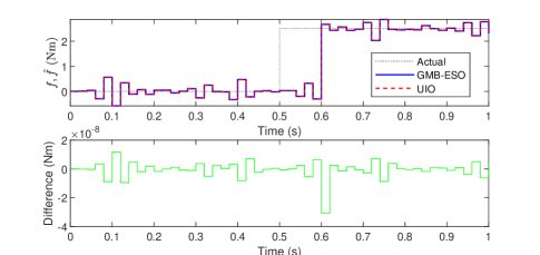
Figure 1: The actual total disturbance and its estimations by GMB-ESO and UIO

Moreover, GMB-ESO can smooth the estimation of the total disturbance. In motion control, the sample time is usually $1$ ms. After discretizing the SEA with this sample time, the discretized system is given by the matrices $A_{0}=\begin{bmatrix}0&1&0&0\\ -0.9793&1.9793&1.056e-6&0\\ 0&0&0&1\\ 0.0046&0&-0.9991&1.9989\end{bmatrix},B_{0}=\begin{bmatrix}0\\ 0\\ 0\\ 0.1904\end{bmatrix},$ $C_{0}=[1,0,0,0],E_{0}=[0,0,0,1]^{T}.$

Since the sample time is very small and the UIO tries to derive a very accurate total disturbance to let the plant follow the polluted measurements quickly, the estimated total disturbance of UIO is very large as shown in the top of Fig. 2. So, the UIO cannot be used in the case when the measurement noise is large and the sample time is small. However, by adjusting the observer bandwidth $\omega_{o}$, GMB-ESO has the ability to smooth the estimated total disturbance. Fig. 2 shows that the lower the observer bandwidth is, the smoother the estimated total disturbance acts, the slower the estimated total disturbance follows the actual total disturbance.

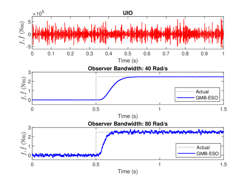
Figure 2: The estimated total disturbances using UIO and GMB-ESO with different observer bandwidth

IV GMB-ESO with Built-In Zero Dynamics

In this section, GMB-ESO with built-in zero dynamics is proposed for a SISO linear system. To make the design method of ESO clearer, the nominal model of conventional ESO, i.e., the observability canonical form, is firstly reviewed systematically.

System (1) considered in the preceding sections only takes into account a single total disturbance. However, real-world plants may be subject to numerous internal and external disturbances. Only inputs and outputs of the plant are available. We need to find a nominal model to represent the actual plant as close as possible.

Consider the following nominal SISO system given by

$$\begin{cases}x(k+1)=A_{0}x(k)+B_{0}u(k)+D_{0}d(k)\\ y(k)=C_{0}x(k)\end{cases}$$ (33)

where $d\in\mathbb{R}^{q}$ is the unknown disturbance vector including internal and external disturbances, and $D_{0}\in\mathbb{R}^{n\times q}$. Assumption 1 is satisfied. Note that $E_{0}f(k)$ in system (1) is replaced by $D_{0}d(k)$ as $f$ represents the total disturbance but $d$ denotes the actual internal and external disturbances.

IV-A An Unsolved Problem in ESO Design

Under Assumption 1, if there are no disturbances, a SISO linear system can be transformed to a normal form by using the following invertible matrix [30]

$$T_{1}=\begin{bmatrix}C_{0}\\ \vdots\\ C_{0}A_{0}^{r-1}\\ \Phi\end{bmatrix},$$ (34)

where $\Phi\in\mathbb{R}^{m\times n}$, $\Phi B_{0}=0$, and $r\triangleq n-m$ is the relative degree. Since the relative degree is $r$, we have

$$\begin{array}[]{r@{}l}C_{0}A_{0}^{i-1}B_{0}=&0\quad\text{for all}\quad i=1,\cdots,r-1\\ C_{0}A_{0}^{r-1}B_{0}\neq&0.\end{array}$$ (35)

Due to the existence of disturbances in system (33), we set

$$\begin{bmatrix}\zeta(k)\\ \eta(k)\end{bmatrix}=T_{1}x(k)+\begin{bmatrix}M\\ 0_{m\times(r-1)q}\end{bmatrix}\boldsymbol{d}(k),$$ (36)

where $\boldsymbol{d}(k)=[d(k)^{T},d(k+1)^{T},\cdots,d(k+r-2)^{T}]^{T}$, $M=\begin{bmatrix}0&0&\cdots&0\\ C_{0}D_{0}&0&\cdots&0\\ C_{0}A_{0}D_{0}&C_{0}D_{0}&\cdots&0\\ \vdots&\vdots&\ddots&\vdots\\ C_{0}A_{0}^{r-2}D_{0}&C_{0}A_{0}^{r-3}D_{0}&\cdots&C_{0}D_{0}\end{bmatrix}$, $\zeta\in\mathbb{R}^{r}$, and $\eta\in\mathbb{R}^{m}$. For convenience, let $T_{1}^{-1}\triangleq[T_{1a},T_{1b}]$, where $T_{1a}\in\mathbb{R}^{n\times r}$ and $T_{1b}\in\mathbb{R}^{n\times m}$.

From (36), we have an expression of $x$ in terms of $\zeta$, $\eta$ and $\boldsymbol{d}$. Substituting this $x$ and (35) into system (33) yields the following normal form

$$\begin{cases}\zeta(k+1)=\hat{A}_{0}\zeta(k)+\hat{B}_{0}u(k)+\hat{E}_{0}(\hat{F}_{0}\eta(k)+f_{1}(k))\\ \eta(k+1)=\hat{S}_{0}\eta(k)+\hat{G}_{0}\zeta(k)+d_{\eta}(k)\\ y(k)=\hat{C}_{0}\zeta(k)\end{cases}$$ (37)

where $\hat{A}_{0}=\begin{bmatrix}0&1&\cdots&0\\ \vdots&\vdots&\ddots&\vdots\\ 0&0&\cdots&1\\ \alpha_{1}&\alpha_{2}&\cdots&\alpha_{r}\end{bmatrix}$, $\hat{B}_{0}=\begin{bmatrix}0\\ \vdots\\ 0\\ b_{0}\end{bmatrix}$, $\hat{E}_{0}=\begin{bmatrix}0\\ \vdots\\ 0\\ 1\end{bmatrix}$,

$[\alpha_{1},\cdots,\alpha_{r}]\triangleq C_{0}A_{0}^{r}T_{1a}$, $b_{0}=C_{0}A_{0}^{r-1}B_{0}$, $\hat{F}_{0}=C_{0}A_{0}^{r}T_{1b}$, $\hat{C}_{0}=[1,0,\cdots,0]$, $\hat{S}_{0}=\Phi A_{0}T_{1b}$, $f_{1}(k)=\sum\limits_{i=1}^{r}C_{0}A_{0}^{r-i}D_{0}d(k+i-1)-C_{0}A_{0}^{r}T_{1a}M\boldsymbol{d}(k)$, $\hat{G}_{0}=\Phi A_{0}T_{1a}$, $d_{\eta}(k)=\Phi D_{0}d(k)-\Phi A_{0}T_{1a}M\boldsymbol{d}(k)$. The total disturbance in conventional ESO design is defined as

$$f_{a}(k)=\hat{F}_{0}\eta(k)+f_{1}(k).$$ (38)

As shown in system (37), the zero dynamics is separated from the observability canonical form. There are no invariant zeros between $f_{a}$ and $y$, in which $f_{a}$ is composed of $\hat{F}_{0}\eta$ from zero dynamics and $f_{1}$ from the model uncertainty and external disturbances. Therefore, the information of zero dynamics cannot be added into the observer design.

IV-B Adding Given Zero Dynamics to GMB-ESO

To add zero dynamics in ESO design, we set

$$\bar{x}(k)=T_{2}x(k)+P\bar{\boldsymbol{d}}(k),$$ (39)

where $P=\begin{bmatrix}0&0&\cdots&0\\ C_{0}D_{0}&0&\cdots&0\\ C_{0}A_{0}D_{0}&C_{0}D_{0}&\cdots&0\\ \vdots&\vdots&\ddots&\vdots\\ C_{0}A_{0}^{n-2}D_{0}&C_{0}A_{0}^{n-3}D_{0}&\cdots&C_{0}D_{0}\end{bmatrix}$, $T_{2}=[C_{0}^{T},\cdots,(C_{0}A_{0}^{n-1})^{T}]^{T}$, $\bar{\boldsymbol{d}}(k)=[d(k)^{T},d(k+1)^{T},\cdots,d(k+n-2)^{T}]^{T}$.

From (39), we have an expression of $x$ in terms of $\bar{x}$ and $\bar{\boldsymbol{d}}$. Substituting this $x$ into system (33) yields the following observability canonical form

$$\begin{cases}\bar{x}(k+1)=\bar{A}_{0}\bar{x}(k)+\bar{B}_{0}u(k)+\bar{E}_{0}f_{b}(k)\\ y(k)=\bar{C}_{0}\bar{x}(k)\end{cases}$$ (40)

where $\bar{A}_{0}=T_{2}A_{0}T_{2}^{-1}$, $\bar{B}_{0}=T_{2}B_{0}$, $\bar{C}_{0}=C_{0}T_{2}^{-1}$, $\bar{E}_{0}=[0,\cdots,0,1]^{T}$, and the total disturbance in GMB-ESO is

$$f_{b}(k)=\sum\limits_{i=1}^{n}C_{0}A_{0}^{n-i}D_{0}d(k+i-1)-C_{0}A_{0}^{n}T_{2}^{-1}P\bar{\boldsymbol{d}}(k).$$ (41)

System (40) can be converted back to the original form (33) with the total disturbance $f_{b}$ added as follows:

$$\begin{cases}\tilde{x}(k+1)=A_{0}\tilde{x}(k)+B_{0}u(k)+E_{0}f_{b}(k)\\ y(k)=C_{0}\tilde{x}(k)\end{cases}$$ (42)

where $E_{0}=T_{2}^{-1}\bar{E}_{0}$ and $\tilde{x}=T_{2}^{-1}\bar{x}$.

Since there are no invariant zeros between $y$ and $f_{b}$, an observer (6) of augmented system of system (42) can be used to estimate $\tilde{x}$ and $f_{b}$. Comparing (38) and (41), it is clear that the known zero dynamics is no longer a part of the total disturbance to be estimated, thereby greatly reducing the load on the observer.

Remark 6

For multi-output systems, the observability matrix can be easily obtained if the system is observable. Therefore, the method proposed above can be generalized to multi-input multi-output (MIMO) systems. Moreover, ESO-like methods have already been generalized to MIMO systems [31, 32].

V Concluding Remarks

To address the problem of uncertainties, the well-established ESO design principle is extended in this paper to the plants rigorously studied in the existing mathematical control theory: single-input single-output linear time-invariant systems with a given state space model. The proposed GMB-ESO provides effective means to estimate both the state and the lumped disturbance, i.e., the total disturbance, where the data of the combined effects of unmodeled dynamics and external disturbances on the plant is obtained in real time. Such information, needless to say, is critical in allowing the rich body of knowledge in modern control theory to be directly applicable to engineering practice where uncertainties abound.

In particular, the mature and rigorous body of work on UIO functions as a bridge in this paper to help analytically establish and numerically verify the proposed approach. First, Lemma 1 shows that the condition for convergence of ESO in continuous-time systems [23] is equivalent to Assumption 2, i.e., no invariant zeros exist between the plant output and the total disturbance. Secondly, Theorem 1 shows that UIO sets the ceiling, a theoretical limit, for the performance of GMB-ESO, and that GMB-ESO can reach this ceiling only if its bandwidth ($\omega_{o}$) is pushed to be infinite and Assumption 2 holds. In addition, as Theorem 2 implies the output of GMB-ESO can be made as smooth as needed by adjusting $\omega_{o}$ in the presence of measurement noise. Furthermore, the closed-form error-bound for the estimation of the total disturbance $f$ is obtained and shown to be monotonically decreasing as the bandwidth $\omega_{o}$ increases. Finally, a particular form of GMB-ESO with built-in zero dynamics is introduced for those plants with zeros between the input and output, which have been left untreated in all existing ESO designs. Including zero dynamics in ESO reduces the load on ESO by incorporating into it the known dynamics and not wasting its bandwidth.

References

• [1] K. J. Åström and P. R. Kumar, “Control: A perspective.” Automatica, vol. 50, no. 1, pp. 3–43, 2014.
• [2] T. Samad, “A survey on industry impact and challenges thereof [technical activities],” IEEE Control Systems Magazine, vol. 37, no. 1, pp. 17–18, 2017.
• [3] J. Han, “Active disturbance rejection controller and its application,” Control and Decision, vol. 13, no. 1, pp. 19–23, 1998 [in Chinese].
• [4] ——, “From pid to active disturbance rejection control,” IEEE transactions on Industrial Electronics, vol. 56, no. 3, pp. 900–906, 2009.
• [5] Y. Huang and W. Xue, “Active disturbance rejection control: Methodology and theoretical analysis,” ISA transactions, vol. 53, no. 4, pp. 963–976, 2014.
• [6] X. Zhang, X. Zhang, W. Xue, and B. Xin, “An overview on recent progress of extended state observers for uncertain systems: Methods, theory, and applications,” Advanced Control for Applications: Engineering and Industrial Systems, vol. 3, no. 2, p. e89, 2021.
• [7] I. The MathWorks, Simulink Control Design Toolbox, Natick, Massachusetts, United State, 2022b. [Online]. Available: https://www.mathworks.com/help/slcontrol/ug/active-disturbance-rejection-control.html
• [8] W. Xue, S. Chen, C. Zhao, Y. Huang, and J. Su, “On integrating uncertainty estimator into pi control for a class of nonlinear uncertain systems,” IEEE Transactions on Automatic Control, vol. 66, no. 7, pp. 3409–3416, 2021.
• [9] K. Łakomy and R. Madonski, “Cascade extended state observer for active disturbance rejection control applications under measurement noise,” ISA transactions, vol. 109, pp. 1–10, 2021.
• [10] M. Ran, J. Li, and L. Xie, “A new extended state observer for uncertain nonlinear systems,” Automatica, vol. 131, p. 109772, 2021.
• [11] S. Li, J. Yang, W.-H. Chen, and X. Chen, “Generalized extended state observer based control for systems with mismatched uncertainties,” IEEE Transactions on Industrial Electronics, vol. 59, no. 12, pp. 4792–4802, 2012.
• [12] M. Hou and R. Patton, “Optimal filtering for systems with unknown inputs,” IEEE Transactions on Automatic Control, vol. 43, no. 3, pp. 445–449, 1998.
• [13] M. L. Hautus, “Strong detectability and observers,” Linear Algebra and its applications, vol. 50, pp. 353–368, 1983.
• [14] A. Ansari and D. S. Bernstein, “Deadbeat unknown-input state estimation and input reconstruction for linear discrete-time systems,” Automatica, vol. 103, pp. 11–19, 2019.
• [15] S. Sundaram and C. N. Hadjicostis, “Delayed observers for linear systems with unknown inputs,” IEEE Transactions on Automatic Control, vol. 52, no. 2, pp. 334–339, 2007.
• [16] A. Chakrabarty, R. Ayoub, S. H. Żak, and S. Sundaram, “Delayed unknown input observers for discrete-time linear systems with guaranteed performance,” Systems & Control Letters, vol. 103, pp. 9–15, 2017.
• [17] A. Chakrabarty, M. J. Corless, G. T. Buzzard, S. H. Żak, and A. E. Rundell, “State and unknown input observers for nonlinear systems with bounded exogenous inputs,” IEEE Transactions on Automatic Control, vol. 62, no. 11, pp. 5497–5510, 2017.
• [18] H. Kong and S. Sukkarieh, “An internal model approach to estimation of systems with arbitrary unknown inputs,” Automatica, vol. 108, p. 108482, 2019.
• [19] D. Ichalal and S. Mammar, “On unknown input observers of linear systems: Asymptotic unknown input decoupling approach,” IEEE Transactions on Automatic Control, vol. 65, no. 3, pp. 1197–1202, 2020.
• [20] A. S. Khan, A. Q. Khan, N. Iqbal, G. Mustafa, M. A. Abbasi, and A. Mahmood, “Design of a computationally efficient observer-based distributed fault detection and isolation scheme in second-order networked control systems,” ISA transactions, vol. 128, pp. 229–241, 2022.
• [21] M. Hou and P. C. Müller, “Design of decentralized linear state function observers,” Automatica, vol. 30, no. 11, pp. 1801–1805, 1994.
• [22] M. A. Abooshahab, M. M. Alyaseen, R. R. Bitmead, and M. Hovd, “Simultaneous input & state estimation, singular filtering and stability,” Automatica, vol. 137, p. 110017, 2022.
• [23] W. Bai, S. Chen, Y. Huang, B.-Z. Guo, and Z.-H. Wu, “Observers and observability for uncertain nonlinear systems: A necessary and sufficient condition,” International Journal of Robust and Nonlinear Control, vol. 29, no. 10, pp. 2960–2977, 2019.
• [24] Z. Gao, “Scaling and bandwidth-parameterization based controller tuning,” in American Control Conference, 2003, pp. 4989–4996.
• [25] M. E. Valcher, “State observers for discrete-time linear systems with unknown inputs,” IEEE Transactions on Automatic Control, vol. 44, no. 2, pp. 397–401, 1999.
• [26] W. Xue and Y. Huang, “Performance analysis of active disturbance rejection tracking control for a class of uncertain lti systems,” ISA transactions, vol. 58, pp. 133–154, 2015.
• [27] L. B. Freidovich and H. K. Khalil, “Performance recovery of feedback-linearization-based designs,” IEEE Transactions on Automatic Control, vol. 53, no. 10, pp. 2324–2334, 2008.
• [28] A. Alan, T. G. Molnar, E. Daş, A. D. Ames, and G. Orosz, “Disturbance observers for robust safety-critical control with control barrier functions,” IEEE Control Systems Letters, vol. 7, pp. 1123–1128, 2023.
• [29] J. Chen, Y. Hu, and Z. Gao, “On practical solutions of series elastic actuator control in the context of active disturbance rejection,” Advanced Control for Applications: Engineering and Industrial Systems, vol. 3, no. 2, p. e69, 2021.
• [30] A. Isidori, Nonlinear control systems, 3rd ed.   Berlin: Springer, 1995.
• [31] L. Wang, A. Isidori, and H. Su, “Output feedback stabilization of nonlinear mimo systems having uncertain high-frequency gain matrix,” Systems & Control Letters, vol. 83, pp. 1–8, 2015.
• [32] Y. Wu, A. Isidori, R. Lu, and H. K. Khalil, “Performance recovery of dynamic feedback-linearization methods for multivariable nonlinear systems,” IEEE Transactions on Automatic Control, vol. 65, no. 4, pp. 1365–1380, 2020.