DPAUC: Differentially Private AUC Computation in Federated Learning
Abstract
Federated learning (FL) has gained significant attention recently as a privacy-enhancing tool to jointly train a machine learning model by multiple participants. The prior work on FL has mostly studied how to protect label privacy during model training. However, model evaluation in FL might also lead to potential leakage of private label information. In this work, we propose an evaluation algorithm that can accurately compute the widely used AUC (area under the curve) metric when using the label differential privacy (DP) in FL. Through extensive experiments, we show our algorithms can compute accurate AUCs compared to the ground truth. The code is available at https://github.com/bytedance/fedlearner/tree/master/example/privacy/DPAUC
Introduction
With increasing concerns over data privacy in machine learning, regulations like CCPA111California Consumer Privacy Act, HIPAA222Health Insurance Portability and Accountability Act, and GDPR333General Data Protection Regulation, European Union have been introduced to regulate how data can be transmitted and used. To address privacy concerns, federated learning (McMahan et al. 2017; Hanzely et al. 2020; Yuan and Ma 2020; Ghosh et al. 2020) has become an increasingly popular tool to enhance privacy by allowing training models without directly sharing their data. Depending on how data is split across parties, FL can be mainly classified into two categories (Yang et al. 2019a): Horizontal Federated Learning (Geiping et al. 2020; Hamer, Mohri, and Suresh 2020; Karimireddy et al. 2020; Li et al. 2020) and Vertical Federated Learning (Vepakomma et al. 2018a; Gupta and Raskar 2018; Abuadbba et al. 2020; Ceballos et al. 2020). In Horizontal FL (hFL), data is split by entity (e.g. a person), and data entities owned by each party are disjointed from other parties. In Vertical FL (vFL), a data entity is split into different attributes (e.g. features and labels of the same person), and each party might own the same data entities but their different attributes. In this paper, we focus on the setting of hFL which enables devices (i.e. mobile phones) to collaboratively learn a machine learning model (i.e. binary classifier) while keeping all the training and testing data on the device.
Although raw data is not shared in federated learning, sensitive information may still be leaked when gradients and/or model parameters are communicated between parties. In hFL, (Zhu, Liu, and Han 2019) showed that an honest-but-curious server can uncover the raw features and labels of a device by knowing the model architecture, parameters, and communicated gradient of the loss on the device’s data. Based on their techniques, (Zhao, Mopuri, and Bilen 2020) showed that the ground truth label of an example can be extracted by exploiting the directions of the gradients of the weights connected to the logits of different classes. Researchers have shown that vFL can still leak data information indirectly. For example, (Li et al. 2022) demonstrated that the gradient norms and directions can leak label information in the two-party vFL setting. However, the prior work on FL privacy mostly focuses on model training and there can also be privacy leaks from model evaluation. Specifically, the private label information owned by clients/devices can be leaked to the server when computing evaluation metrics in FL.
Previous work (Matthews and Harel 2013a) has shown that releasing the actual ROC curves on a private test dataset can allow an attacker with some prior knowledge of the test dataset to recover some sensitive information about the dataset. Some recent works(Chen et al. 2016; Stoddard, Chen, and Machanavajjhala 2014) proposed to provide differential privacy (DP) for plotting and releasing ROC curves. However, they have several challenges such as how to privately compute the true positive rate (TPR) and false positive rate (FPR) values and how many and what thresholds to pick(Stoddard, Chen, and Machanavajjhala 2014). And they are not designed and applicable for evaluating FL models. As the ground-truth labels often contain highly sensitive information (e.g., whether a user has purchased (in online advertising) or whether a user has a disease or not (in disease prediction) (Vepakomma et al. 2018b; Li et al. 2022), it cannot be directly shared between clients and servers, and clients and clients. Hence preventing the label leakage from the AUC computation in the general setting of FL is challenging.
To address the challenge, we consider the area under the Receiver operating characteristic (ROC) curve as the target AUC to evaluate the accuracy of a binary classifier. Since the class label is often the most sensitive information in a prediction task, our goal in this paper is to achieve label differential privacy (Ghazi et al. 2021) while plotting the ROC curve. To this end, we propose to adopt the Laplace mechanism 444Other mechanisms such as the Gaussian mechanism are applicable too) to add noise to the shared intermediate information between the server and clients to plot the Receiver operating characteristic (ROC) curve and calculate the area under the ROC curve as the AUC. We conduct extensive experiments to demonstrate the effectiveness of our proposed approach.
Preliminaries
We focus on the setting of hFL which contains one server and multi-clients (devices). The labels are distributed in multi clients and our proposed approach can compute the evaluation metric AUC with label differential privacy. We start by introducing some background knowledge of our work.
Label Differential Privacy
Differential privacy (DP) (Dwork et al. 2006; Dwork and Roth 2014a) is a quantifiable and rigorous privacy framework. We adopt the following definition of DP. We define Differential privacy (DP) (Dwork et al. 2006; Dwork and Roth 2014a) as the following:
Definition 0.1 (Differential Privacy).
Let , a randomized mechanism is -differentially private (i.e. -DP), if for any of two neighboring training datasets , and for any subset of the possible output of , we have
If , then is -differentially private (i.e. -DP).
In our work, we focus on protecting the privacy of label information. Following (Ghazi et al. 2021), we define label differential privacy as the following:
Definition 0.2 (Label Differential Privacy).
Let , a randomized mechanism is -label differentially private (i.e. -LabelDP), if for any of two neighboring training datasets that differ in the label of a single example, and for any subset of the possible output of , we have
If , then is -label differentially private (i.e. -LabelDP).
Our proposed approach also shares the same setting with local DP (Duchi, Jordan, and Wainwright 2013; Erlingsson, Pihur, and Korolova 2014; Kasiviswanathan et al. 2008; Bebensee 2019) which assumes that the data collector (server in our paper) is untrusted. Following the same setting with local DP, in our proposed approach, each client locally perturbs their sensitive information with a DP mechanism and transfers the perturbed version to the server. After receiving all clients’ perturbed data, the server calculates the statistics and publishes the result of AUC. We define local DP as the following:
Definition 0.3 (Local Differential Privacy).
Let and , a randomized mechanism is -local differentially private (i.e. -LocalDP), if and only if for any pair of input values and in domain , and for any subset of possible output of , we have
If , then is -local differentially private (i.e. -LocalDP).
Definition 0.4 (Sensitivity).
Let be a positive integer, be a collection of datasets, and be a function. The sensitivity of a function, denoted , is defined by where the maximum is over all pairs of datasets and in differing in at most one element and denotes the norm.
Definition 0.5 (Laplace Mechanism ).
Laplace mechanism defined by (Dwork and Roth 2014b) preserves -differential privacy if the random noise is drawn from the Laplace distribution with parameter , where is the sensitivity and , is the corresponding privacy budget.
In this paper, we leverage two DP properties (Dwork and Roth 2014b; McSherry and Talwar 2007) to help us build a complex workflow that still has the DP guarantee: sequential composition and postprocessing. Let and be and differentially private algorithms, sequential composition guarantees that releasing the outputs of and satisfies DP. Postprocessing an output of a DP algorithm does not incur any additional loss of privacy. For example, releasing and still satisfies DP.
ROC Curve and AUC
In a binary classification problem, given a threshold , a predicted score is predicted to be if . Given the ground-truth label and the predicted label (at a given threshold ), we can quantify the accuracy of the classifier on the dataset with True positives (TP()), False positives (FP()), False negatives (FN()), and True negatives (TN()).
-
•
True positives, TP(), are the data points in the test whose true label and predicted label equal . i.e. and
-
•
False positives, FP(), are the data points in test whose true label is but the predicted label is . i.e. and .
-
•
False negatives, FN(), are data points whose true label is but the predicted label is . i.e. and .
-
•
True negatives, TN(), are data points whose true label is and the predicted label is . i.e. and .
The area under the receiver operating characteristic (ROC) curves plots TPR (x-axis) vs. FPR (y-axis) over all possible thresholds , and AUC is the area under the ROC curve. True Positive Rate (TPR) (i.e. recall) is defined as and False Positive Rate (FPR) is defined as . If the classifier is good, the ROC curve will be close to the left and upper boundary and AUC will be close to (a perfect classifier). On the other hand, if the classifier is poor, the ROC curve will be close to the line from to with AUC around (random prediction).
Privacy Leakage in AUC.
Researchers have shown AUC computation can cause privacy leakage. Matthews and Harel (Matthews and Harel 2013b) demonstrate that by using a subset of the ground-truth data and the computed ROC curve, the data underlying the ROC curve can be reproduced accurately. Stoddard el al. (Stoddard, Chen, and Machanavajjhala 2014) show that an attacker can determine the unknown label by simply enumerating over all labels, guessing the labels, and then checking which guesses lead to the given ROC curve. They propose a differentially private ROC curve computation algorithm. They first privately choose a set of thresholds (with privacy budget ). By modeling TP and FP values as one-sided range queries, they can compute noisy TPRs and FPRs values (using privacy budget ). They also leveraged a postprocessing step to enforce the monotonicity of TPRs and FPRs. However, the above method is not designed for FL settings. In this paper, we aim to provide a differentially private way to compute AUC in the FL setting.
Threat Model
In our hFL setting, there are multiple label parties (i.e. clients/devices) that own private labels (i.e. Y) and there is a central non-label party (i.e. server) that is responsible for computing global AUC from all clients. The model is trained using the normal hFL protocol.
Our work focuses on the evaluation time and the goal of the server is to compute global AUC without letting clients directly share their private test data. In other words, clients cannot directly send the test data (i.e. private labels and prediction scores) to the server for it to compute AUC. Specifically, we are interested in protecting label information and therefore it is required that the exchanged information between client and server excludes the ground-truth test labels (Y) and corresponding prediction scores.
Methods
In this section, we introduce how to compute the AUC with label differential privacy by leveraging the Laplace mechanism. Here we use the Laplace mechanism as an example. Settings for other DP mechanisms such as the Gaussian mechanism will be the same.
Overall Workflow
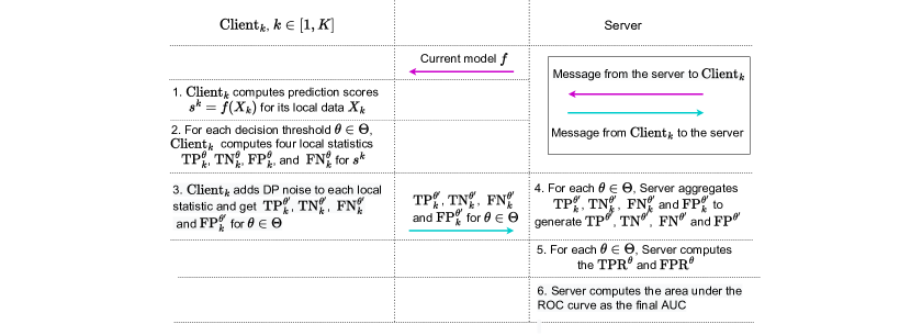
The workflow of this method is shown in Figure 1. The algorithm has six steps:
-
1.
Clients Execute. Each client computes the prediction scores for all its owning data points.
-
2.
Clients Execute. For each decision threshold , client computes four local statistics ,,, and given the prediction scores .
-
3.
Clients Executes. The client adds perturbation with DP guarantee to each local statistics ,,, and and get corresponding noisy statistics ,,, and for each . Client sends all noisy statistics to the server.
-
4.
Server Executes. For each , the server aggregates the noisy statistics from all the clients: ,,, and
-
5.
Server Executes. For each , the server computes the corresponding and .
-
6.
Server Executes. The server plots TPR (x-axis) vs. FPR (y-axis) over all possible thresholds and computes the area under the corresponding curve as AUC.
Adding DP Noise to Local Statistics
In this section, we explain in details on how to perturb TP, TN,FP, and FN for each in each client. It’s worth mentioning that both Gaussian and Laplace mechanisms can be leveraged to generate the corresponding DP noise. Without loss of generality, we use Laplace as an example. Laplace mechanism preserves -differential privacy if the random noise is drawn from the Laplace distribution with parameter where is the sensitivity (Dwork and Roth 2014b) and is the corresponding privacy budget. We name this method as . The noise is added as the following:
-
1.
Adding noise to TP: Each client sets the corresponding sensitivity for each . Given a privacy budget , client draws the random noise from and add it to and get .
-
2.
Adding noise to FP: Each client sets the corresponding sensitivity for each . Given a privacy budget , client draws the random noise from and add it to and get .
-
3.
Adding noise to TN: Each client sets the corresponding sensitivity for each . Given a privacy budget , client draws the random noise from and add it to and get .
-
4.
Adding noise to FN: Each client sets the corresponding sensitivity for each . Given a privacy budget , client draws the random noise from and add it to and get .
Privacy Analysis. Based on the Composition Theorem of DP (Dwork and Roth 2014b), the privacy budget for each decision boundary () is (). Since we have decision thresholds (), the total DP privacy budget is . Without loss of generality, we set in our paper and the total DP budget is .
Experiments
In this section, we show the experimental results of evaluating our proposed approaches. We introduce the experimental setups first.
| RR | ||||||
|---|---|---|---|---|---|---|
| epoch | Tensorflow | scikit-learn | =8.0 | =4.0 | =2.0 | =1.0 |
| 0 | 0.749357 | 0.749383 | 0.74938 0.00004 | 0.749398 0.0004 | 0.749108 0.000932 | 0.750239 0.001766 |
| 1 | 0.766434 | 0.766477 | 0.766447 0.000054 | 0.766338 0.000338 | 0.7665588 0.001109 | 0.766392 0.002098 |
| 2 | 0.770189 | 0.770219 | 0.770204 0.000049 | 0.770112 0.000375 | 0.7702048 0.000795 | 0.771098 0.001891 |
Experimental Setup
Dataset. We evaluate the proposed approaches on Criteo 555https://www.kaggle.com/c/criteo-display-ad-challenge/data, which is a large-scale industrial binary classification dataset (with approximately million user click records) for conversion prediction tasks. Every record of Criteo has categorical input features and real-valued input features. We first replace all the NA values in categorical features with a single new category (which we represent using the empty string) and replace all the NA values in real-valued features with . For each categorical feature, we convert each of its possible value uniquely to an integer between (inclusive) and the total number of unique categories (exclusive). For each real-valued feature, we linearly normalize it into . We then randomly sample of the entire Criteo set as our training data and the remaining as our test data. We computed the AUC on the test set which contains where and for epochs.
Model. We modified a popular deep learning model architecture WDL (Cheng et al. 2016) for online advertising. Note that our goal is not to train the model that can beat the state-of-the-art, but to test the effectiveness of our proposed federated AUC computation approach.
Ground-truth AUC. We compare our proposed DPAUC with two AUC computation libraries (their computed results work as ground-truth and have no privacy guarantee): 1) scikit-learn666https://scikit-learn.org/stable/modules/generated/sklearn.metrics.auc.html; 2) Tensorflow 777https://www.tensorflow.org/api˙docs/python/tf/keras/metrics/AUC. Both approximate the AUC (Area under the curve) of the ROC. In our experiments, we set for Tensorflow. We use the default values for other parameters.
Evaluation Metric. For each method, we run the same setting for times (change the random seed every time) and use the corresponding mean and standard deviation of the computed AUC as our evaluation metric. A good computation method should achieve a small std of the computed AUC and the corresponding mean value of the computed AUC should be close to the ground-truth AUC.
One Randomized Responses based Competitor:
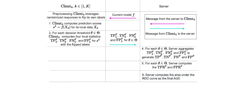
We introduce another algorithm to compute AUC for evaluating FL models as one competitor. The algorithm is based on randomized response (Warner 1965) and we name it as . We include the workflow in Figure 2. We now explain the algorithm step by step.
Step 1: Clients Flip Their Local Labels
Randomized response (RR) is -LabelDP (Ma and Wang 2021; Xiong et al. 2020) and works as follows: let be a parameter and let be the true label. Given a query of , RR will respond with a random draw from the following probability distribution:
| (1) |
Clients leverage randomized responses to flip their owning labels as a preprocessing step before computing the AUC. It’s worth mentioning that all labels are only flipped once and the generated noisy labels can then be used for further evaluations multi-times.
Step 2: Server Computes AUC from Flipped Labels
Since the corresponding AUC is computed with flipped labels, we denote this AUC as noisy AUC: . It has the same six steps as DPAUC except that each client computes local statistics with flipped labels and sends the corresponding results (without adding additional noises) to the server.
Step 3: Server Debiases AUC
We leveraged (Menon et al. 2015) to debiase the noisy AUC and get the final clean AUC that we are interested in.
Utility and Privacy Analysis
The corresponding results of can be seen in Table 1. However, has potential privacy issues since the prediction scores can be inferred from the change of adjacent local statistics. For example, we can conclude that there are some prediction scores that fall in if there are some differences between (, , , ) and (, , , ) from client .
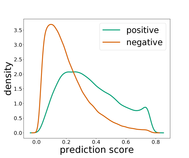
Attackers can then infer the label information based on the exposed prediction scores. We propose a simple attack method to infer the label information based on the prediction scores. The strategy of the attack is to select the samples with top-K prediction scores as positive labels. We measure the corresponding guessing performance by precision and recall. As shown in Figure 3 and Table 2, positive instances can have relatively higher prediction scores than negative ones at some density areas. For example, we can achieve a precision if we select the instances with top- prediction scores. Hence, exposing prediction scores among all participants can increase the risk of label leakage. However, since the prediction scores are shuffled before sending to the server, the server has no idea which prediction score belongs to which data sample 888.
| Top K | Positives in Top K | Precision | Recall |
|---|---|---|---|
| 1 | 1 | 1 | 8.52e-6 |
| 5 | 4 | 0.8 | 3.41e-5 |
| 10 | 8 | 0.8 | 6.82e-5 |
| 50 | 43 | 0.86 | 3.67e-4 |
| 100 | 79 | 0.79 | 6.73e-4 |
| 500 | 384 | 0.768 | 3.27e-3 |
| 1,000 | 774 | 0.774 | 6.60e-3 |
| 5,000 | 3,914 | 0.7828 | 0.0334 |
| 10,000 | 7,519 | 0.7519 | 0.0641 |
| 50,000 | 30,793 | 0.6159 | 0.2625 |
| 100,000 | 52,268 | 0.5227 | 0.4455 |
To prevent label leakage from the prediction scores, we may leverage DP to add noise to the prediction scores. Since the prediction score is the output of a softmax/sigmoid function, the corresponding sensitivity . We can then leverage the Laplace mechanism 999The Gaussian mechanism can be applied here too to add corresponding noise to the prediction scores. The corresponding results can be seen in Table 3. We can observe that the utility of the computed AUC is highly sensitive to the privacy budget of the prediction scores. We cannot even achieve a reasonable AUC utility with a small (i.e. ) of prediction scores. The results show that is not a suitable procedure to achieve a good tradeoff between utility and privacy for computing AUC in FL.
| Epoch | 0 | 1 | 2 | |
|---|---|---|---|---|
| Tensorflow | 0.7494 | 0.7665 | 0.7702 | |
| scikit-learn | 0.7494 | 0.7665 | 0.7702 | |
| 1 | 0.5374 | 0.5416 | 0.5420 | |
| 2 | 0.5725 | 0.5795 | 0.5830 | |
| 3 | 0.5976 | 0.6105 | 0.6130 | |
| 4 | 0.6239 | 0.6367 | 0.6387 | |
| 5 | 0.6413 | 0.6569 | 0.6607 | |
| 6 | 0.6571 | 0.6732 | 0.6786 | |
| 7 | 0.6698 | 0.6870 | 0.6903 | |
| 8 | 0.6797 | 0.6976 | 0.7022 | |
| 9 | 0.6885 | 0.7060 | 0.7115 | |
| 10 | 0.6952 | 0.7124 | 0.7191 | |
| 50 | 0.7454 | 0.7625 | 0.7663 | |
| 100 | 0.7484 | 0.7654 | 0.7692 | |
| 1000 | 0.7494 | 0.7665 | 0.7702 |
Experimental Results of
We now introduce the experimental results of and demonstrate the effectiveness of .
IID vs. Non-IID
Based on the setting of how to assign data samples to clients, we provide two simulations to conduct the corresponding experiments.
-
1.
IID: all data points are uniformly assigned to the clients.
-
2.
Non-IID: all data points are assigned to the clients based on their corresponding prediction scores. Data samples with similar prediction scores will be assigned to the same client.
| epoch | Tensorflow | scikit-learn | =0.02, =8 | =0.01, =4 | =0.005, =2 | =0.0025,=1 | |
| 0 | 0.749357 | 0.749383 | IID, | 0.749347 0.000216 | 0.749178 0.000484 | 0.748937 0.000755 | 0.748206 0.001649 |
| Non-IID, | 0.749319 0.000242 | 0.749260 0.000474 | 0.749192 0.00072 | 0.748962 0.00178 | |||
| IID, | 0.74811 0.002335 | 0.745557 0.004498 | 0.738944 0.008008 | 0.726187 0.014704 | |||
| Non-IID, | 0.748062 0.001981 | 0.746105 0.004465 | 0.741711 0.009246 | 0.726885 0.016539 | |||
| 1 | 0.766434 | 0.766477 | IID, | 0.766373 0.000239 | 0.766309 0.000402 | 0.76611 0.000894 | 0.765684 0.001677 |
| Non-IID, | 0.766378 0.000231 | 0.766197 0.000471 | 0.76612 0.000755 | 0.765447 0.001805 | |||
| IID, | 0.764887 0.002241 | 0.763012 0.004378 | 0.756938 0.008096 | 0.740619 0.017457 | |||
| Non-IID, | 0.764923 0.002036 | 0.763246 0.004022 | 0.756715 0.009105 | 0.744978 0.018234 | |||
| 2 | 0.770189 | 0.770219 | IID, | 0.770091 0.000258 | 0.769995 0.000498 | 0.770028 0.000788 | 0.769143 0.00172 |
| Non-IID, | 0.770095 0.000213 | 0.770115 0.000434 | 0.76981 0.000903 | 0.769265 0.001502 | |||
| IID, | 0.76918 0.002519 | 0.766482 0.004387 | 0.761074 0.007947 | 0.745812 0.014596 | |||
| Non-IID, | 0.768894 0.002104 | 0.766819 0.003802 | 0.759916 0.007251 | 0.746815 0.016511 |
We divide data samples into clients based on the IID and Non-IID settings and each client has data samples on average. We set and compare the difference between IID and Non-IID settings for and in Table 4. We can observe that our method can achieve similar performance (mean and standard deviation of computed AUC) under both IID and Non-IID settings. It indicates that our proposed method is robust to Non-IID settings.
Effects of Number of Samples per Client
Given the fixed total number of data points (), is sensitive to the number of clients or the number of samples per client has. We vary the number of data samples per client owing and conduct experiments with (around data points per client) and (around data points per client). The corresponding results are shown in Table 4. We can conclude that with an increasing avg. data samples per client, can achieve a smaller standard deviation of AUC estimation since it adds relatively small amounts of noise to the local statistics and hence has fewer effects on the computational results.
Effects of Number of Decision Boundaries
We also conducted experiments to test the effects of the number of decision boundaries (). The corresponding experiments are performed with IID setting with . We tested as shown in Table 5. Given the same privacy budget , with increasing , each local statistic has to be assigned a smaller privacy budget (adding more DP noise). As a result, the standard deviation of the computed AUC will be smaller for smaller . However, smaller can have a worse effect on the computed precision of the resulted AUC. In our experiments, we found can achieve a good performance on both precision and standard deviation of the AUC.
| epoch | Tensorflow | scikit-learn | |||||
|---|---|---|---|---|---|---|---|
| 0 | 0.749357 | 0.749383 | 10 | 0.7251052 0.000074 | 0.725064 0.000167 | 0.725008 0.000323 | 0.724899 0.000607 |
| 25 | 0.747879 0.000147 | 0.747895 0.000275 | 0.747669 0.000625 | 0.747278 0.000889 | |||
| 50 | 0.748914 0.000161 | 0.748884 0.000343 | 0.748988 0.000657 | 0.748816 0.001279 | |||
| 100 | 0.749347 0.000216 | 0.749178 0.000484 | 0.748937 0.000755 | 0.748206 0.001649 | |||
| 200 | 0.74929 0.000289 | 0.74916 0.000573 | 0.748491 0.001204 | 0.747117 0.002224 | |||
| 1 | 0.766434 | 0.766477 | 10 | 0.744348 0.000084 | 0.744317 0.000144 | 0.744215 0.000328 | 0.744058 0.000639 |
| 25 | 0.765178 0.000159 | 0.765045 0.000252 | 0.7649144 0.000507 | 0.764968 0.001282 | |||
| 50 | 0.766198 0.000187 | 0.766181 0.000329 | 0.765973 0.000723 | 0.766009 0.001216 | |||
| 100 | 0.766373 0.000239 | 0.766309 0.000402 | 0.76611 0.000894 | 0.765684 0.001677 | |||
| 200 | 0.76638 0.000311 | 0.766235 0.000677 | 0.765694 0.001367 | 0.764399 0.002264 | |||
| 2 | 0.770189 | 0.770219 | 10 | 0.748858 0.000073 | 0.7487984 0.000123 | 0.748821 0.000331 | 0.748626 0.000591 |
| 25 | 0.769006 0.000162 | 0.768992 0.000323 | 0.768705 0.000508 | 0.768357 0.001308 | |||
| 50 | 0.769806 0.000220 | 0.769756 0.000500 | 0.769549 0.000805 | 0.76939 0.001034 | |||
| 100 | 0.770091 0.000258 | 0.769995 0.000498 | 0.770028 0.000788 | 0.769143 0.00172 | |||
| 200 | 0.770137 0.000319 | 0.769729 0.000633 | 0.769066 0.001085 | 0.767694 0.002746 |
Related Work
Federated Learning. FL (McMahan et al. 2017; Yang et al. 2019b) can be mainly classified into three categories: horizontal FL, vFL, and federated transfer learning (Yang et al. 2019b). In this paper, we focus on hFL which partitions data by entities.
Information Leakage in FL. Recently, studies show that in FL, even though the raw data (feature and label) is not shared, sensitive information can still be leaked from the gradients and intermediate embeddings communicated between parties. For example, (Vepakomma et al. 2019) and (Sun et al. 2021) showed that server’s raw features can be leaked from the forward cut layer embedding. In addition, (Li et al. 2022) studied the label leakage problem but the leakage source was the backward gradients rather than forward embeddings. (Zhu, Liu, and Han 2019) showed that an honest-but-curious server can uncover the raw features and labels of a device by knowing the model architecture, parameters, and communicated gradient of the loss on the device’s data. Based on their techniques, (Zhao, Mopuri, and Bilen 2020) showed that the ground truth label of an example can be extracted by exploiting the directions of the gradients of the weights connected to the logits of different classes.
Information Protection in FL. There are three main categories of information protection techniques in FL: 1) cryptographic methods such as secure multi-party computation (Bonawitz et al. 2017); 2) system-based methods including trusted execution environments (Subramanyan et al. 2017); and 3) perturbation methods that add noise to the communicated messages (Abadi et al. 2016; McMahan et al. 2018; Erlingsson et al. 2019; Cheu et al. 2019; Zhu, Liu, and Han 2019). In this paper, we focus on adding DP noise to protect the private label information during computing AUC in FL.
Conclusion
In this paper, we focus on providing label differential privacy for computing AUC during the model evaluation in the setting of hFL. We proposed an approach with label DP to compute AUC for evaluating models. We conducted extensive experiments to verify the effectiveness of our proposed methods. We use the Laplace mechanism as an example. Other DP mechanisms such as the Gaussian mechanism can be applied to our framework too. In our current design, the privacy budget of is linear with the query times (model evaluation times on the same evaluation set). As future work, we may leverage the strong composition property of DP (Dwork, Rothblum, and Vadhan 2010; Gopi, Lee, and Wutschitz 2021) to reduce the privacy budget from linear to square root.
References
- Abadi et al. (2016) Abadi, M.; Chu, A.; Goodfellow, I.; McMahan, H. B.; Mironov, I.; Talwar, K.; and Zhang, L. 2016. Deep learning with differential privacy. In Proceedings of the 2016 ACM SIGSAC Conference on Computer and Communications Security, 308–318.
- Abuadbba et al. (2020) Abuadbba, S.; Kim, K.; Kim, M.; Thapa, C.; Camtepe, S. A.; Gao, Y.; Kim, H.; and Nepal, S. 2020. Can We Use Split Learning on 1D CNN Models for Privacy Preserving Training? In Proceedings of the 15th ACM Asia Conference on Computer and Communications Security, 305–318.
- Bebensee (2019) Bebensee, B. 2019. Local Differential Privacy: a tutorial. CoRR, abs/1907.11908.
- Bonawitz et al. (2017) Bonawitz, K.; Ivanov, V.; Kreuter, B.; Marcedone, A.; McMahan, H. B.; Patel, S.; Ramage, D.; Segal, A.; and Seth, K. 2017. Practical secure aggregation for privacy-preserving machine learning. In Proceedings of the 2017 ACM SIGSAC Conference on Computer and Communications Security, 1175–1191.
- Ceballos et al. (2020) Ceballos, I.; Sharma, V.; Mugica, E.; Singh, A.; Roman, A.; Vepakomma, P.; and Raskar, R. 2020. SplitNN-driven Vertical Partitioning. arXiv preprint arXiv:2008.04137.
- Chen et al. (2016) Chen, Y.; Machanavajjhala, A.; Reiter, J. P.; and Barrientos, A. F. 2016. Differentially Private Regression Diagnostics. In 2016 IEEE 16th International Conference on Data Mining (ICDM), 81–90.
- Cheng et al. (2016) Cheng, H.-T.; Koc, L.; Harmsen, J.; Shaked, T.; Chandra, T.; Aradhye, H.; Anderson, G.; Corrado, G.; Chai, W.; Ispir, M.; et al. 2016. Wide & deep learning for recommender systems. In Proceedings of the 1st workshop on deep learning for recommender systems, 7–10.
- Cheu et al. (2019) Cheu, A.; Smith, A.; Ullman, J.; Zeber, D.; and Zhilyaev, M. 2019. Distributed differential privacy via shuffling. In Annual International Conference on the Theory and Applications of Cryptographic Techniques, 375–403. Springer.
- Duchi, Jordan, and Wainwright (2013) Duchi, J. C.; Jordan, M. I.; and Wainwright, M. J. 2013. Local Privacy and Statistical Minimax Rates. In 2013 IEEE 54th Annual Symposium on Foundations of Computer Science, 429–438.
- Dwork et al. (2006) Dwork, C.; McSherry, F.; Nissim, K.; and Smith, A. 2006. Calibrating noise to sensitivity in private data analysis. In Theory of cryptography conference, 265–284. Springer.
- Dwork and Roth (2014a) Dwork, C.; and Roth, A. 2014a. The algorithmic foundations of differential privacy. Found. Trends Theor. Comput. Sci., 9(3-4): 211–407.
- Dwork and Roth (2014b) Dwork, C.; and Roth, A. 2014b. The Algorithmic Foundations of Differential Privacy. Found. Trends Theor. Comput. Sci., 9(3–4): 211–407.
- Dwork, Rothblum, and Vadhan (2010) Dwork, C.; Rothblum, G. N.; and Vadhan, S. 2010. Boosting and Differential Privacy. In 2010 IEEE 51st Annual Symposium on Foundations of Computer Science, 51–60.
- Erlingsson et al. (2019) Erlingsson, Ú.; Feldman, V.; Mironov, I.; Raghunathan, A.; Talwar, K.; and Thakurta, A. 2019. Amplification by shuffling: From local to central differential privacy via anonymity. In Proceedings of the Thirtieth Annual ACM-SIAM Symposium on Discrete Algorithms, 2468–2479. SIAM.
- Erlingsson, Pihur, and Korolova (2014) Erlingsson, Ú.; Pihur, V.; and Korolova, A. 2014. RAPPOR: Randomized Aggregatable Privacy-Preserving Ordinal Response. In Ahn, G.; Yung, M.; and Li, N., eds., Proceedings of the 2014 ACM SIGSAC Conference on Computer and Communications Security, Scottsdale, AZ, USA, November 3-7, 2014, 1054–1067. ACM.
- Geiping et al. (2020) Geiping, J.; Bauermeister, H.; Dröge, H.; and Moeller, M. 2020. Inverting Gradients - How easy is it to break privacy in federated learning? In Larochelle, H.; Ranzato, M.; Hadsell, R.; Balcan, M. F.; and Lin, H., eds., Advances in Neural Information Processing Systems, volume 33, 16937–16947. Curran Associates, Inc.
- Ghazi et al. (2021) Ghazi, B.; Golowich, N.; Kumar, R.; Manurangsi, P.; and Zhang, C. 2021. On Deep Learning with Label Differential Privacy. arXiv preprint arXiv:2102.06062.
- Ghosh et al. (2020) Ghosh, A.; Chung, J.; Yin, D.; and Ramchandran, K. 2020. An Efficient Framework for Clustered Federated Learning. In Larochelle, H.; Ranzato, M.; Hadsell, R.; Balcan, M. F.; and Lin, H., eds., Advances in Neural Information Processing Systems, volume 33, 19586–19597. Curran Associates, Inc.
- Gopi, Lee, and Wutschitz (2021) Gopi, S.; Lee, Y. T.; and Wutschitz, L. 2021. Numerical Composition of Differential Privacy. In Ranzato, M.; Beygelzimer, A.; Dauphin, Y.; Liang, P.; and Vaughan, J. W., eds., Advances in Neural Information Processing Systems, volume 34, 11631–11642. Curran Associates, Inc.
- Gupta and Raskar (2018) Gupta, O.; and Raskar, R. 2018. Distributed learning of deep neural network over multiple agents. Journal of Network and Computer Applications, 116: 1–8.
- Hamer, Mohri, and Suresh (2020) Hamer, J.; Mohri, M.; and Suresh, A. T. 2020. FedBoost: A Communication-Efficient Algorithm for Federated Learning. In III, H. D.; and Singh, A., eds., Proceedings of the 37th International Conference on Machine Learning, volume 119 of Proceedings of Machine Learning Research, 3973–3983. PMLR.
- Hanzely et al. (2020) Hanzely, F.; Hanzely, S.; Horváth, S.; and Richtarik, P. 2020. Lower Bounds and Optimal Algorithms for Personalized Federated Learning. In Larochelle, H.; Ranzato, M.; Hadsell, R.; Balcan, M. F.; and Lin, H., eds., Advances in Neural Information Processing Systems, volume 33, 2304–2315. Curran Associates, Inc.
- Karimireddy et al. (2020) Karimireddy, S. P.; Kale, S.; Mohri, M.; Reddi, S.; Stich, S.; and Suresh, A. T. 2020. SCAFFOLD: Stochastic Controlled Averaging for Federated Learning. In III, H. D.; and Singh, A., eds., Proceedings of the 37th International Conference on Machine Learning, volume 119 of Proceedings of Machine Learning Research, 5132–5143. PMLR.
- Kasiviswanathan et al. (2008) Kasiviswanathan, S. P.; Lee, H. K.; Nissim, K.; Raskhodnikova, S.; and Smith, A. D. 2008. What Can We Learn Privately? CoRR, abs/0803.0924.
- Li et al. (2022) Li, O.; Sun, J.; Yang, X.; Gao, W.; Zhang, H.; Xie, J.; Smith, V.; and Wang, C. 2022. Label Leakage and Protection in Two-party Split Learning. In The Tenth International Conference on Learning Representations (ICLR).
- Li et al. (2020) Li, Z.; Kovalev, D.; Qian, X.; and Richtarik, P. 2020. Acceleration for Compressed Gradient Descent in Distributed and Federated Optimization. In III, H. D.; and Singh, A., eds., Proceedings of the 37th International Conference on Machine Learning, volume 119 of Proceedings of Machine Learning Research, 5895–5904. PMLR.
- Ma and Wang (2021) Ma, F.; and Wang, P. 2021. Randomized Response Mechanisms for Differential Privacy Data Analysis: Bounds and Applications. CoRR, abs/2112.07397.
- Matthews and Harel (2013a) Matthews, G.; and Harel, O. 2013a. An Examination of Data Confidentiality and Disclosure Issues Related to Publication of Empirical ROC Curves. Academic radiology, 20: 889–96.
- Matthews and Harel (2013b) Matthews, G. J.; and Harel, O. 2013b. An examination of data confidentiality and disclosure issues related to publication of empirical ROC curves. Academic Radiology, 20(7): 889–896.
- McMahan et al. (2017) McMahan, B.; Moore, E.; Ramage, D.; Hampson, S.; and y Arcas, B. A. 2017. Communication-efficient learning of deep networks from decentralized data. In Artificial Intelligence and Statistics, 1273–1282. PMLR.
- McMahan et al. (2018) McMahan, H. B.; Ramage, D.; Talwar, K.; and Zhang, L. 2018. Learning Differentially Private Recurrent Language Models. In International Conference on Learning Representations.
- McSherry and Talwar (2007) McSherry, F.; and Talwar, K. 2007. Mechanism Design via Differential Privacy. In 48th Annual IEEE Symposium on Foundations of Computer Science (FOCS’07), 94–103.
- Menon et al. (2015) Menon, A.; Rooyen, B. V.; Ong, C. S.; and Williamson, B. 2015. Learning from Corrupted Binary Labels via Class-Probability Estimation. In Bach, F.; and Blei, D., eds., Proceedings of the 32nd International Conference on Machine Learning, volume 37 of Proceedings of Machine Learning Research, 125–134. Lille, France: PMLR.
- Stoddard, Chen, and Machanavajjhala (2014) Stoddard, B.; Chen, Y.; and Machanavajjhala, A. 2014. Differentially Private Algorithms for Empirical Machine Learning. CoRR, abs/1411.5428.
- Subramanyan et al. (2017) Subramanyan, P.; Sinha, R.; Lebedev, I.; Devadas, S.; and Seshia, S. A. 2017. A formal foundation for secure remote execution of enclaves. In Proceedings of the 2017 ACM SIGSAC Conference on Computer and Communications Security, 2435–2450.
- Sun et al. (2021) Sun, J.; Yao, Y.; Gao, W.; Xie, J.; and Wang, C. 2021. Defending against Reconstruction Attack in Vertical Federated Learning. CoRR, abs/2107.09898.
- Vepakomma et al. (2019) Vepakomma, P.; Gupta, O.; Dubey, A.; and Raskar, R. 2019. Reducing leakage in distributed deep learning for sensitive health data. arXiv preprint arXiv:1812.00564.
- Vepakomma et al. (2018a) Vepakomma, P.; Gupta, O.; Swedish, T.; and Raskar, R. 2018a. Split learning for health: Distributed deep learning without sharing raw patient data. arXiv preprint arXiv:1812.00564.
- Vepakomma et al. (2018b) Vepakomma, P.; Gupta, O.; Swedish, T.; and Raskar, R. 2018b. Split learning for health: Distributed deep learning without sharing raw patient data. arXiv preprint arXiv:1812.00564.
- Warner (1965) Warner, S. L. 1965. Randomized Response: A Survey Technique for Eliminating Evasive Answer Bias. Journal of the American Statistical Association, 60(309): 63–69.
- Xiong et al. (2020) Xiong, X.; Liu, S.; Li, D.; Cai, Z.; Niu, X.; and Del Rey, A. M. 2020. A Comprehensive Survey on Local Differential Privacy. Sec. and Commun. Netw., 2020.
- Yang et al. (2019a) Yang, Q.; Liu, Y.; Chen, T.; and Tong, Y. 2019a. Federated machine learning: Concept and applications. ACM Transactions on Intelligent Systems and Technology (TIST), 10(2): 1–19.
- Yang et al. (2019b) Yang, Q.; Liu, Y.; Chen, T.; and Tong, Y. 2019b. Federated machine learning: Concept and applications. In ACM Transactions on Intelligent Systems and Technology (TIST), 1–19. ACM New York, NY, USA.
- Yuan and Ma (2020) Yuan, H.; and Ma, T. 2020. Federated Accelerated Stochastic Gradient Descent. In Larochelle, H.; Ranzato, M.; Hadsell, R.; Balcan, M. F.; and Lin, H., eds., Advances in Neural Information Processing Systems, volume 33, 5332–5344. Curran Associates, Inc.
- Zhao, Mopuri, and Bilen (2020) Zhao, B.; Mopuri, K. R.; and Bilen, H. 2020. iDLG: Improved Deep Leakage from Gradients. arXiv preprint arXiv:2001.02610.
- Zhu, Liu, and Han (2019) Zhu, L.; Liu, Z.; and Han, S. 2019. Deep leakage from gradients. In Advances in Neural Information Processing Systems, 14774–14784.