Finding of a population of active galactic nuclei showing a significant luminosity decline in the past $\sim 10^{3-4}$ yrs

Abstract

Recent observations have revealed an interesting active galactic nuclei (AGN) subclass that shows strong activity at large scales ($\sim 1$ kpc) but weaker at small scales ($<10$ pc), suggesting a strong change in the mass accretion rate of the central engine in the past $10^{3-4}$ yr. We systematically search for such declining or fading AGN by cross-matching the SDSS type-1 AGN catalog at $z<0.4$, covering the [O iii]$\lambda 5007$ emission line which is a tracer for the narrow-line region (NLR) emission, with the WISE mid-infrared (MIR) catalog covering the emissions from the dusty tori. Out of the 7,653 sources, we found 57 AGN whose bolometric luminosities estimated from the MIR band are at least one order of magnitude fainter than those estimated from the [O iii]$\lambda 5007$ emission line. This luminosity declining AGN candidate population shows four important properties: 1) the past AGN activity estimated from the [O iii]$\lambda 5007$ line reaches around the Eddington-limit, 2) more than 30% of the luminosity declining AGN candidates show a large absolute variability of $\Delta W1>0.45$ mag in the previous $\sim 10$ yr at the WISE 3.4 $\mu$m band, 3) the median ratio of $\log$([N ii]$\lambda 6584/\mathrm{H}\alpha\lambda 6563)=-0.52$, suggesting a lower gas metallicity and/or higher ionization parameter compared to other AGN populations. 4) the second epoch spectra of the population indicate a spectral type change for 15% of the sources. This population provides insights on the possible connection between the luminosity decline which started $\sim 10^{3-4}$ yr ago and the decline in the recent $10$ yr.

1 Introduction

One big question in the astronomy is on how super massive black holes (SMBH) increase their mass across the cosmic epoch in the universe. Active galactic nuclei (AGN) are a key population for the SMBH growth since they are in a rapidly growing state of their BH masses through the gas accretion to the central SMBHs, until they reach the redshift-independent maximum mass limit at $M_{\mathrm{max}}\sim$ a few $\times 10^{10}M_{\odot}$ (Netzer, 2003; Kormendy & Ho, 2013). This indicates that SMBHs and their accretion systems might have a self-regulating process that shuts down the growth of SMBHs before reaching a certain maximum mass ($\leq M_{\mathrm{max}}$) (Natarajan & Treister, 2009; King, 2016; Inayoshi & Haiman, 2016).

One of the biggest unknowns for this accretion process is how long such an AGN phase lasts. Several studies indicate that the total lifetime of the AGN is $\sim 10^{7-9}$ yr (Soltan, 1982; Marconi et al., 2004) and even the single episode has a length of $>10^{5}$ yr (Schawinski et al., 2015) and likely around $10^{6-7}$ yr (Marconi et al., 2004; Hopkins et al., 2006), which is still orders of magnitude longer than one person’s lifetime of $\sim 10^{2}$ yr.

One way to expand the AGN variability window beyond the human lifetime is to compare the activity of the different physical scales of the AGN, as the shutdown process propagates from the inner regions to the outer ones with the light crossing time (e.g., see Ichikawa & Tazaki, 2017a). In the scale of 10 to 100 gravitational radius ($R_{\mathrm{g}}$) away from the SMBH, the X-ray emitting corona and UV–optically bright accretion disk (AD) is located (Dai et al., 2010; Morgan et al., 2010), 0.1-10 pc the mid-infrared (MIR) bright tori (Burtscher et al., 2013), and $\sim 10^{3-4}$ pc the narrow line region (NLR; Bennert et al., 2002). Using those AGN components with different physical scales enables us to explore the long-term luminosity variability with the order of $\sim 10^{3-4}$ yr. Recent studies have revealed that there are certain populations of AGN with strong activity in large scales but weaker ones in the small scales, which suggests a strong decline of the accretion rate into the central SMBHs. These AGN are called fading or dying AGN. Currently roughly $>30$ of such fading AGN (candidates) were reported (Schirmer et al., 2013; Ichikawa et al., 2016; Kawamuro et al., 2017; Keel et al., 2017; Villar-Martín et al., 2018; Sartori et al., 2018; Wylezalek et al., 2018; Ichikawa et al., 2019a, b; Chen et al., 2019, 2020b, 2020a; Esparza-Arredondo et al., 2020; Saade et al., 2022).

In this paper, we conduct a systematic search of such luminosity declining AGN by combining the SDSS AGN catalog with the WISE MIR all-sky survey. The SDSS AGN catalog of Mullaney et al. (2013) contains 25,670 AGN with the [O iii]$\lambda 5007$ emission line, which is one of the large scale AGN indicators with $\sim$kpc scale. WISE enables us to obtain the warm dust emission heated by AGN, which is one of the small physical scale AGN indicators with $\sim 1$ pc scale. The combination of these two AGN indicator information enables us to obtain the long-term AGN variability of $\sim 10^{3-4}$ yr timescale. Throughout this paper, we adopt the same cosmological parameters as Mullaney et al. (2013); $H_{0}=71$ km s^-1 Mpc^-1, $\Omega_{\mathrm{M}}=0.27$, and $\Omega_{\Lambda}=0.73$.

2 Sample and Selection

2.1 SDSS Type 1 AGN of Mullaney et al. (2013)

Our initial parent sample starts from the AGN catalog compiled by Mullaney et al. (2013), which includes 25,670 optically selected active galactic nuclei (AGN) from the SDSS DR7 data release (Abazajian et al., 2009) at $z<0.4$, where H$\alpha$ is within the SDSS wavelength coverage. Mullaney et al. (2013) conducted their own spectral fitting of the SDSS spectra including the narrow components of the narrow H$\beta$ and H$\alpha$ emission lines, which gives better fitting results for the emission lines compared to the original SDSS fitting method which applied a more simplified fitting (e.g., York et al., 2000; Abazajian et al., 2009).

In this study, we used only type-1 AGN from the Mullaney et al. (2013) catalog for searching luminosity declining AGN because of the two reasons; 1) the more reliable observed [O iii]$\lambda 5007$ luminosities with small extinctions considering their viewing angle (e.g., Antonucci, 1993) and 2) availability of $M_{\rm BH}$ measurements thanks to the existence of the broad emission lines. Mullaney et al. (2013) classified AGN as type-1 if they fulfill the following criteria for their H$\alpha$-line: 1) an extra Gaussian (for the broad component) in addition to the narrow Gaussian provides a significantly better fit, 2) the broad component flux exceeds the narrow one, and 3) FWHM of broad H$\alpha$ component has $>600$ km s^-1.

The obtained type-1 AGN catalog contains 9,455 sources and it provides the emission line fluxes, redshifts, and luminosities of [O iii]$\lambda 5007$, H$\alpha$, H$\beta$, and [N ii]$\lambda 6584$, and the obtained fluxes are separated into narrow and broad components, as well as the physical values based on those emission line measurements, such as black hole masses ($M_{\rm BH}$), and Eddington ratio ($\lambda_{\mathrm{Edd}}$), both of which are estimated based on the broad H$\alpha$ emission lines (Greene & Ho, 2005).

We then limited our sample to the sources with reliable spectral fitting. First, we limit our samples to low extinction values for the narrow-line region with $A_{\mathrm{V}}<10$, since otherwise the luminosities of these sources are unrealistically over-estimated (see Mullaney et al., 2013, for more details). This reduces the sample into 9,372 sources. Second, we limit the sources whose [O iii]$\lambda 5007$ emission line is significantly detected, with a signal to noise ratio of $\mathrm{S/N}\geq 5$. The resulting type-1 AGN sample contains 7,755 sources.

It should be pointed out that searching only for type-1 luminosity declining AGN significantly reduces the possibility for finding genuine “dying” AGN whose central engine is completely quenched, such as Arp 187 (Ichikawa et al., 2019a, b), which is likely classified as type-2 AGN in the optical spectra because of the lack of the broad emission lines already in the current SDSS spectra. We will explore luminosity declining/dying type-2 AGN systematic search in the forthcoming paper.

2.2 Cross-matching with WISE

The WISE mission mapped the entire sky in 3.4 $\mu$m (W1), 4.6 $\mu$m (W2), 12 $\mu$m (W3), and 22 $\mu$m (W4) bands (Wright et al., 2010; Wright, 2010a). In this study, we obtained the data from the latest ALLWISE catalog (Cutri et al., 2013). We used the pipeline measured magnitudes at the W3-band based on the PSF-profile fitting on $\sim 6$ arcsec scale, called profile fitting magnitude and w3mpro in the WISE catalog terminology. The positional accuracy based on cross-matching with the 2MASS catalog is $\sim 2$ arcsec at the $3\sigma$ level (e.g., see Ichikawa et al., 2012, 2017), and we also applied the 2 arcsec cross-matching radius between the SDSS optical coordinates and WISE. This reduces the sample from 7,755 to 7,723 sources.

We obtained the W3-band fluxes and treated the value as detection for the sources with ph_qual=A,B,C, with SN higher than 2. The ph_qual=U were treated as upper limit detection since we are looking for low luminosity AGN in the MIR band and it is therefore also important to consider the weak detections in the MIR bands for our parent sample. We also applied the contamination-free sources with ccflag=0. This reduces the sample to 7,653, where 6,028/1,496/75/54 of the sources have the photometric quality of ph_qual=A/B/C/U, respectively. We refer to this sample as “parent sample” for searching the luminosity declining AGN.

2.3 AGN Luminosities and Bolometric Corrections

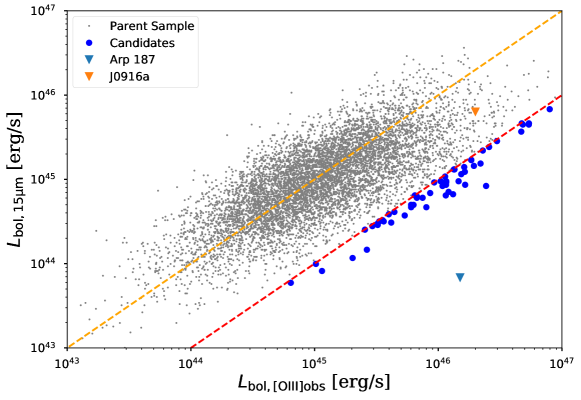
Figure 1: The correlation of the bolometric AGN luminosity estimated from the WISE 12 $\mu$m band and [O iii]$\lambda 5007$  emission line. The gray dot represents the parent sample and the blue filled circle represents the luminosity declining AGN candidates. The orange dashed line represents the 1:1 line of the two luminosities. For the comparison with other fading/dying AGN, we showed the location of Arp 187 (blue uppe-bound), which is one of the most promising dying AGN (Ichikawa et al., 2016; Ichikawa & Tazaki, 2017b; Ichikawa et al., 2019a, b) and the location of J0916a (orange upper-bound), which is a fading AGN whose fading phase is likely recently started ($<10^{2}$ yr) with strong past outburst activity in the NLR (Chen et al., 2019, 2020b, 2020a). The selection criteria of the luminosity declining AGN candidates discussed in section 1 is represented by the red dashed line.

We measured the AGN bolometric luminosities based on the obtained AGN indicators tracing different physical scales. For the NLR luminosities tracing a $\sim 10^{3-4}$ pc scale, we utilized the observed [O iii]$\lambda 5007$ luminosities obtained by Mullaney et al. (2013) and then applied the constant bolometric correction of $L_{\rm bol,[OIII]obs}=3500L_{\mathrm{[OIII]obs}}$ with the median error of 0.38 dex (e.g., Heckman et al., 2004). We note that our sample contains [OIII] luminous AGN that are not covered in Heckman et al. (2004), notably the sources with $L_{\mathrm{[OIII]obs}}\geq 10^{42.5}$ erg s^-1. We here apply the same constant bolometric correction even for those sources since the overall spectral shape does not change in the standard disk regime even when the accretion rate changes (Kato et al., 2008). One might also wonder that the bolometric correction might change in the super-Eddington regime. We will discuss this point later in Section 3.2. Another point is that Mullaney et al. (2013) already provide the bolometric luminosities of the sample by utilizing the extinction corrected [O iii]$\lambda 5007$ luminosities. However, we did not use those since they are often unrealistically large values exceeding $L_{\rm bol,[OIII]obs}>10^{48}$ erg s^-1, which is the Eddington limit of the mass of $M_{\mathrm{BH}}\sim 10^{10}M_{\odot}$; the known maximum mass limit of the SMBHs.

For the AGN dust luminosities tracing $\sim 10$ pc scale, we first derived the rest-frame 15 $\mu$m luminosities by applying the $k$-correction from the obtained WISE 12 $\mu$m flux density. The rest-frame 15 $\mu$m flux density was extrapolated from the obtained observed 12 $\mu$m flux density with the assumption of AGN IR spectral template of Mullaney et al. (2011) and with the obtained redshift. The AGN bolometric luminosities from the AGN dust were finally estimated from the bolometric correction curve by Hopkins et al. (2007), which has a typical bolometric correction value of $L_{\rm bol,15\mu m}\sim 10L_{\rm 15\mu m}$ with a scatter of a factor of 2.

In addition, we also measured the bolometric AGN luminosities from the accretion disk emission by using the rest-frame B-band continuum fluxes, tracing $\sim 100R_{\mathrm{g}}$ scale assuming the standard thin-disk accretion (e.g., Kato et al., 2008). The B-band fluxes were calculated from the continuum of the SDSS spectra by Mullaney et al. (2013), and assumed that the continuum is dominated by the AGN accretion disk. For the bolometric correction, we applied the one by Hopkins et al. (2007).

In summary, we obtained the three AGN bolometric luminosities from the NLR, AGN dusty torus, and the accretion disk. Figure 1 shows bolometric luminosity correlation between the one from NLR and the one from AGN dusty torus, showing a rough 1:1 relation each other.

2.4 The Emission Region Size of Each AGN Indicator

We estimate the emitting size of each AGN component by utilizing either theoretical or empirical luminosity-distance relations. The emitting size from the SMBH to the B-band in the optical can be obtained by assuming the standard geometrically thin $\alpha$-disk (e.g., Kato et al., 2008), and it is expressed as

$$\begin{split}D_{\mathrm{AD}}/\mathrm{AU}=886.3\left(\dfrac{\lambda}{4450\mathrm{\AA}}\right)^{4/3}&\left(\dfrac{M_{\mathrm{BH}}}{10^{8}M_{\odot}}\right)^{1/3}\\ &\left(\dfrac{L_{\lambda,\mathrm{bol}}}{10^{46}\mathrm{~{}erg~{}s}^{-1}}\right)^{1/3},\end{split}$$ (1)

here we assume the radiation efficiency $\eta_{\mathrm{rad}}=0.1$ (Soltan, 1982) and $\lambda=4450\mathrm{\AA}$ (B-band) as a tracer of the accretion disk (Malkan & Sargent, 1982).

The size of the MIR dust emission region heated by AGN is obtained by MIR high spatial resolution interferomerty observations (e.g., Kishimoto et al., 2011) and can be written as

$$D_{\mathrm{torus}}/\mathrm{pc}=1.3\left(\dfrac{L_{\rm bol,15\mu m}}{10^{46}\mathrm{~{}erg~{}s}^{-1}}\right)^{0.01}.$$ (2)

The size of the NLR and their AGN luminosity dependence has been studied by several authors (Bennert et al., 2002; Hainline et al., 2013; Husemann et al., 2014). Here we apply the relation between the NLR size and the AGN luminosity by Bae et al. (2017) because they utilized the observed [O iii]$\lambda 5007$  luminosities as a tracer of AGN luminosity, which is suitable for our sample of type-1 AGN. The equation is given as

$$D_{\mathrm{NLR}}/\mathrm{kpc}=2.4\left(\dfrac{L_{\rm bol,[OIII]obs}}{10^{46}\mathrm{~{}erg~{}s}^{-1}}\right)^{0.41}$$ (3)

The median size of the NLR of our parent sample is $D_{\mathrm{NLR}}\sim 1$ kpc, which is consistent with our assumption that NLR is a tracer of the past AGN activity of $10^{3-4}$ yr.

2.5 Selection of luminosity declining AGN Candidates

Table 1: Column descriptions for the table of the selected luminosity declining AGN candidates.

Column	Header Name	Unit	Description
1	OBJID		SDSS DR7 Object ID
2	z		Spectroscopic Redshift
3	ra	°	Right ascension
4	dec	°	Declination
5	SMBH_MASS	$10^{7}M_{\odot}$	$M_{\rm BH}$
6	SMBH_MASS_ERR	$10^{7}M_{\odot}$	$\Delta M_{\rm BH}$
7	F_12um	$10^{-17}$ erg s-1 cm-2	$F_{\mathrm{12}\mu\mathrm{m}}$
8	F_12um_ERR	$10^{-17}$ erg s-1 cm-2	$\Delta F_{\mathrm{12}\mu\mathrm{m}}$
9	L_12um	erg s-1	$L_{12\mu{\rm m}}$
10	L_12um_ERR	erg s-1	$\Delta L_{12\mu{\rm m}}$
11	L_15um_BOLO	erg s-1	$L_{\rm bol,15\mu m}$ estimated for the torus
12	L_15um_BOLO_ERR	erg s-1	$\Delta L_{\rm bol,15\mu m}$ estimated for the torus
13	PH_QUAL_12um		Photometric quality for the 12$\mu$m-band (A:SN$>$10 & 1BSN$>$3 & C:SN$>$2)
14	F_NII	$10^{-17}$ erg s-1 cm-2	$F_{\mathrm{[NII]}}$
15	F_NII_ERR	$10^{-17}$ erg s-1 cm-2	$\Delta F_{\mathrm{[NII]}}$
16	L_NII	erg s-1	$L_{\mathrm{[NII]}}$
17	L_NII_ERR	erg s-1	$\Delta L_{\mathrm{[NII]}}$
18	F_HA	$10^{-17}$ erg s-1 cm-2	$F_{\mathrm{H}\alpha}$
19	F_HA_ERR	$10^{-17}$ erg s-1 cm-2	$\Delta F_{\mathrm{H}\alpha}$
20	L_HA	erg s-1	$L_{\mathrm{H}\alpha}$
21	L_HA_ERR	erg s-1	$\Delta L_{\mathrm{H}\alpha}$
22	F_OIII	$10^{-17}$ erg s-1 cm-2	$F_{\mathrm{[OIII]obs}}$
23	F_OIII_ERR	$10^{-17}$ erg s-1 cm-2	$\Delta F_{\mathrm{[OIII]obs}}$
24	L_OIII	erg s-1	$L_{\mathrm{[OIII]obs}}$
25	L_OIII_ERR	erg s-1	$\Delta L_{\mathrm{[OIII]obs}}$
26	L_OIII_BOLO	erg s-1	$L_{\rm bol,[OIII]obs}$ estimated for the NLR
27	L_OIII_BOLO_ERR	erg s-1	$\Delta L_{\rm bol,[OIII]obs}$ estimated for the NLR
28	F_HB	$10^{-17}$ erg s-1 cm-2	$F_{\mathrm{H}\beta}$
29	F_HB_ERR	$10^{-17}$ erg s-1 cm-2	$\Delta F_{\mathrm{H}\beta}$
30	L_HB	erg s-1	$L_{\mathrm{H}\beta}$
31	L_HB_ERR	erg s-1	$\Delta L_{\mathrm{H}\beta}$
32	F_OPTICAL	$10^{-17}$ erg s-1 cm-2	$F_{\mathrm{\textit{B}-band}}$
33	L_OPTICAL	erg s-1	$L_{\mathrm{\textit{B}-band}}$
34	L_OPTICAL_BOLO	erg s-1	$L_{\rm bol,\textit{B}-band}$ estimated for the accretion disk
35	SIZE_NLR	pc	$D_{\mathrm{NLR}}$
36	SIZE_TORUS	pc	$D_{\mathrm{torus}}$
37	SIZE_AD	pc	$D_{\mathrm{AD}}$
38	EDD_NLR		$\lambda_{\mathrm{Edd}}$ estimated for the NLR out of the [O iii]$\lambda 5007$ line information
39	EDD_TORUS		$\lambda_{\mathrm{Edd}}$ estimated for the torus out of the MIR photometric information
40	EDD_AD		$\lambda_{\mathrm{Edd}}$ estimated for the accretion disk out of the optical photometric information
41	LOG_R		$\log(R)$
42	DELTA_W1	mag	$\Delta W1$
43	MJD_WISE		MJD of the WISE observation
44	MJDSDSS		MJD of the SDSS observation

Note. — Table 1 is published in its entirety in the machine-readable format. All column names, their units, and descriptions are shown here for guidance regarding its form and content.

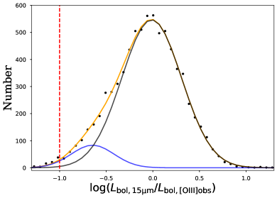
Figure 2: The binned distribution of $\log(R)$ of the parent sample is represented here by the black dotes. The black and blue Gaussian line represents the ones as a result of the two Gaussian component fitting. The orange line represents the composite of the two components. The red line shows the selection cut for the luminosity declining AGN candidates at $\log(R)=-1$.

In order to search for luminosity declining AGN candidates, it is necessary to compare two AGN indicators, a large-scale indicator with a short-scale indicator. NLR is a promising tool as a large-scale AGN indicator because of its large size with $\sim 1-10$ kpc, and the [O iii]$\lambda 5007$ emission line is one of the good indicators of NLR luminosity (Bennert et al., 2002). On the other hand, the emission from the dusty tori is a good AGN indicator tracing smaller physical scale of $\sim 10$ pc (Burtscher et al., 2013; Packham et al., 2005; Radomski et al., 2008; Ramos Almeida et al., 2009; Alonso-Herrero et al., 2011; Ichikawa et al., 2015; Jaffe et al., 2004; Raban et al., 2009; Hönig et al., 2012, 2013; Burtscher et al., 2013; Tristram et al., 2014; López-Gonzaga et al., 2016; Lopez-Rodriguez et al., 2018) and can be traced by the MIR luminosities (e.g., Gandhi et al., 2009a; Ichikawa et al., 2012, 2017, 2019c; Nikutta et al., 2021a, b).

Figure 1 shows the luminosity correlation between the two AGN bolometric luminosities from different AGN indicators, NLR ($\sim$kpc) and dusty tori ($\sim 10$ pc), considered to be tracing the past AGN activities of $\sim 3000$ yr and $\sim 30$ yr ago (Ichikawa & Tazaki, 2017b). Figure 1 shows a one-by-one relation for most of the sample, while some sources have a significantly smaller value at $L_{\rm bol,15\mu m}/L_{\rm bol,[OIII]obs}<0.1$, showing with blue points below the red dashed line.

Figure 2 shows the histogram of the logarithmic ratio $\log(R)$; defined as

$$\log(R)=\log\left(\frac{L_{\rm bol,15\mu m}}{L_{\rm bol,[OIII]obs}}\right).$$ (4)

Here we used the Scott function (Scott, 1979) to define the optimal bin width. We conducted one Gaussian fitting of the histogram of $\log(R)$ and all three parameters (amplitude, mean and standard deviation) were set as free. The fitting still leaves an excess of the distribution at $\log(R)\sim-1$, indicating an additional component, which is also suggested from the blue point sources in Figure 1. We then applied the two Gaussian fitting with all parameters set as free, and the second Gaussian component nicely reproduces the second peak at $\log(R)\sim-0.7$. We also checked the reduced $\chi^{2}$ values of the fittings, with $\chi^{2}_{\nu}=3.5$ for two Gaussians and $\chi^{2}_{\nu}=5.4$ for one Gaussian fitting. This indicates that the distribution can be well described with at least two Gaussian components as shown in Figure 2, and it also suggests that there is a significant peak at $\log(R)\sim-0.7$, which might be related to a population of luminosity declining AGN candidates in this study.

Based on the histogram shown in Figure 2, we selected AGN with $\log(R)<-1$ and we refer to them as “luminosity declining AGN candidates” hereafter. As shown in Figure 1, our selection cut is much more conservative considering the location of another reported fading AGN SDSS J0916a in the plane, which has likely started luminosity decline in the last $<10^{2}$ yr (Chen et al., 2020a). On the other hand, most of our sample spans with $-1.5<\log(R)<-1$, which is one order of magnitude larger value than that of Arp 187, which is a dying AGN, whose central engine is completely quenched. This is also a natural outcome considering that our sample is type-1 AGN whose broad line region still exists, even if they might be in a luminosity declining phase.

As a result, 57 luminosity declining AGN candidates were selected, which is $\sim$0.7% of the parent sample. Table 1 summarizes the list of the physical parameters of the luminosity declining AGN candidates in this study.

3 Results

3.1 Basic Sample Properties

We here summarize the BH properties of the obtained 57 luminosity declining AGN candidates. First, we show the basic differences between the luminosity declining AGN candidates and the parent sample. Then, we show the properties of luminosity declining AGN candidates on the SMBH activities.

3.1.1 AGN Luminosity and Redshift Plane

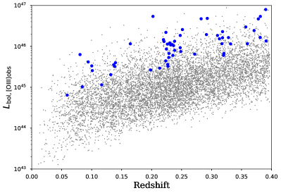
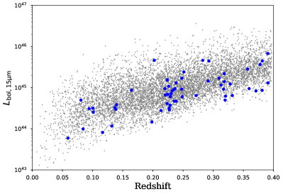
Figure 3: Luminosities of luminosity declining AGN candidates (blue filled circle) and the parent sample (gray dot) as a function of redshift. (Left) The bolometric luminosity estimated from the observed [O iii]$\lambda 5007$ emission luminosities ($L_{\rm bol,[OIII]obs}$) as a function of redshift. (right) The bolometric luminosity estimated from the 15 $\mu$m bands ($L_{\rm bol,15\mu m}$) as a function of redshift.

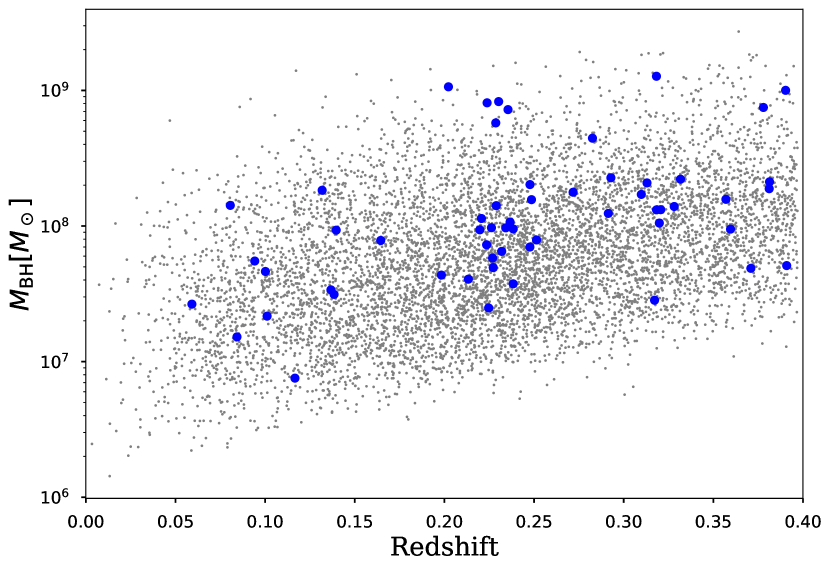
Figure 4: BH mass distribution as a function of redshift. The symbols are the same as in Figure 3.

Figure 3 shows the redshift distributions as a function of $L_{\rm bol,[OIII]obs}$ and $L_{\rm bol,15\mu m}$ for the luminosity declining AGN candidates (blue filled circle) and the parent sample (gray dot). Figure 3 shows two important things. One is that the median $L_{\rm bol,15\mu m}$ of luminosity declining AGN candidates are almost similar to that of the parent sample, while the median $L_{\rm bol,[OIII]obs}$ is one order of magnitude higher than that of the parent sample. This indicates that our luminosity declining AGN candidates had a very luminous AGN phase in the past and we will discuss this part later in Section 4.1.

The second is that our luminosity declining AGN candidates are slightly biased to higher redshift at $z>0.2$. This is partly due to the combination of our selection criteria for selecting large [O iii]$\lambda 5007$ luminosities with $L_{\rm bol,[OIII]obs}>10^{45}$ erg s^-1 as shown in Figure 1, and such sources are a dominant population only at $z>0.2$ as shown in the left panel of Figure 3. Actually, 77% of the luminosity declining AGN candidates are located in a redshift $>0.2$, which is a higher fraction compared to the parent sample (62%). This is also suggested from the difference in the redshift distribution of the two populations (luminosity declining AGN candidates and parent sample), showing the $p$-value of 0.03, suggesting that redshift distribution is slightly skewed to higher redshift for our luminosity declining AGN candidates, and the $p$-value becomes 0.08 if we limit our sample only to sources with $z>0.2$, which suggests a non-significant difference in the distribution (Greenland et al., 2016).

3.1.2 BH Mass and Bolometric Luminosity distributions

The BH mass ($M_{\rm BH}$), one key measurement obtained from the SDSS spectra, is also compiled for all of our samples using the broad H$\alpha$ emission lines (Greene & Ho, 2005), through the spectral fitting done by Mullaney et al. (2013) .

The both population of luminosity declining AGN candidates and the parent sample has a similar median BH mass of $\left<\log(M_{\rm BH}/M_{\odot})\right>=8.0\pm 0.5$ (for luminosity declining AGN candidates) and $\left<\log(M_{\rm BH}/M_{\odot})\right>=7.8\pm 0.5$ (for the parent sample). This suggests that our selection does not show a statistically significant difference on the BH mass as also seen in Figure 4.

3.2 AGN Lightcurves in the last $\sim 10^{4}$ yr

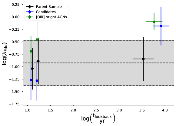
Figure 5: Eddington ratios as a function of the lookback time ($t_{\mathrm{lookback}}$) for luminosity declining AGN candidates, parent sample, and [O iii]$\lambda 5007$ bright AGN. The three lookback times were calculated based on the averaged emitting size of the accretion disks, dusty tori, and the NLRs. Here the dashed lines and grey area represent the median and scatter of the $\lambda_{\mathrm{Edd}}$ of the parent sample. The difference of the observation time between the SDSS DR7 and the WISE observations are taken into account to estimate the $t_{\mathrm{lookback}}$, whose reference time is set on 2022 February 02 (MJD=59612). The $t_{\mathrm{lookback}}$ of the accretion disk and torus for the parent sample are shifted 0.03 dex to the right for clarity.

One of our goals is to obtain how rapidly luminosity declining AGN candidates have experienced the luminosity decline in the last $\sim 3\times 10^{3}$ yrs. To investigate this long-term AGN variability, we estimate the Eddington ratio ($\lambda_{\mathrm{Edd}}\equiv L_{\mathrm{bol}}/L_{\rm Edd}$, where $L_{\rm Edd}$ is Eddington luminosity $L_{\rm Edd}\simeq 1.26\times 10^{38}(M_{\rm BH}/M_{\odot})$ erg s^-1) of our sample. Considering that a few bolometric luminosities are estimated based on the different AGN indicators tracing different physical scales as discussed in Section 2.4, we estimate the Eddington ratio for each AGN indicator.

Figure 5 shows the time evolution of the average Eddington ratio for the luminosity declining AGN candidates and parent sample in the last $\sim 3\times 10^{3}$ yr. The look back time ($t_{\mathrm{lookback}}$) was calculated based on the light crossing time of the three AGN indicators with different physical scales of accretion disk, dusty tori, and NLR (see Section 2.4). We also take into account the different observation dates for the WISE and SDSS observations and we chose 2022 February 2nd (or MJD=59612) as our reference time ($t_{\mathrm{lookback}}$=0). The average MJD of the WISE observation is 55335/55325 for the luminosity declining AGN candidates/parent sample and the average one of the SDSS DR7 is 52997/53046. As a result of the different observation epochs between the WISE and SDSS DR7, the average $t_{\mathrm{lookback}}$ for the accretion disk and dusty tori is the almost same value as shown in Figure 5.

Figure 5 indicates two important things for our luminosity declining AGN candidates and the parent sample. One is that our parent sample shows on average the constant Eddington ratio over the entire time range, that is, the previous $\sim 3\times 10^{3}$ yrs, indicating that the intrinsic variability should be on average smaller than the scatter of $\sim$0.4 dex. This scatter value is consistent with previously known variability strength of typical AGN in the timescale of $\sim 10$ yr (e.g., Hook et al., 1994; Sesar et al., 2007; MacLeod et al., 2010; Kozłowski et al., 2010), and our results suggest that the stochastic variabilities could be within the scatter of 0.4 dex even for the longer timescale of $\sim 10^{3-4}$ yr. This long-term stability of AGN luminosity over the timescale of $\sim 10^{3-4}$ yr is partially suggested from the relation between the X-ray and [O iii]$\lambda 5007$  luminosity correlations of AGN in the local universe, which shows a correlation with the scatter of $\sigma\sim 0.4$ dex (Panessa et al., 2006; Ueda et al., 2015; Berney et al., 2015).

The second is that luminosity declining AGN candidates show a large luminosity decline between the [O iii]$\lambda 5007$ emission region and the torus one, that is, in the previous $\sim 10^{3-4}$ yrs. This is a natural outcome since we set the ratio cut of $R<0.1$. A more interesting trend of the light-curve for luminosity declining AGN candidates is that previous AGN luminosities traced by the [O iii]$\lambda 5007$ emission region have reached almost Eddington limit with $\log\lambda_{\mathrm{Edd}}\sim 0$, while the current Eddington ratio is almost similar with those of the parent sample. This indicates that our fading AGN selection applied for type-1 AGN turn out to be an efficient way to find AGN who experienced the past AGN burst reaching the Eddington limit and this is partially suggested from Figure 3 and Section 3.1.1.

One might wonder that the bolometric correction for [O iii]$\lambda 5007$ line might not be the same values between the standard disk and super-Eddington phase accretion. Although there are no studies on the bolometric corrections including super-Eddington phase, our luminosity declining AGN candidates (and also the parent type-1 AGN sample) do not contain extremely super-Eddington sources reaching $\lambda_{\mathrm{Edd}}\gg 1$, with the maximum value of $\lambda_{\mathrm{Edd}}\simeq 4$ in the NLR. This means that even if the bolometric correction is not constant in the super-Eddington phase, the maximum difference is up to by a factor of 4, and the difference is likely smaller for most of the super-Eddington sources. Therefore, the constant bolometric correction used in this study does not strongly affect main results in this study.

One might also wonder that all Eddington-limit or super-Eddington sources in the [O iii]$\lambda 5007$ emitting region might also have a similar trend of the AGN luminosity declining as seen in the luminosity decline AGN candidates. To check this, we also selected [O iii]$\lambda 5007$ bright AGN that are defined as $\lambda_{\mathrm{Edd}}>0.5$ based on the [O iii]$\lambda 5007$ based AGN bolometric luminosities. This luminosity cut selects the sources with the average value of $\lambda_{\mathrm{Edd}}=$0.8, which is almost consistent with the one of luminosity decline AGN of $\lambda_{\mathrm{Edd}}=0.7$. The green crosses in Figure 5 show the one for [O iii]$\lambda 5007$ bright AGN and they certainly show a slight luminosity decline in the last $10^{3-4}$ yr, while the luminosity decline is smaller than that of luminosity decline AGN candidates. This suggests that higher Eddington sources have a shorter lifetime residing in such a high Eddington ratio phase compared to the one in the lower Eddington ratio, but our luminosity decline AGN might have an additional mechanism to produce such a large luminosity decline reaching a factor of $>10$ in the timescale of $10^{3-4}$ yr.

3.3 IR Variability tracing the past $\sim 10$ yr

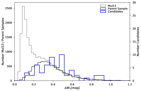
Figure 6: Comparison of the variability distribution of the $\Delta W1$ for luminosity declining AGN candidates in blue, the parent sample in black, and additional to the complete AGN catalog of Mullaney et al. (2013, Mul13) containing also type-2 AGN in grey. The left y-axis shows the number of the sources for the parent sample and the catalog of Mullaney et al. (2013, Mul13) and the right axis shows for the luminosity declining AGN candidates.

It is worthwhile to trace the IR luminosity variability from the dusty torus by using the ALLWISE and NEOWISE IR light curves of W1 and W2-bands covering the last 10 yr (Mainzer et al., 2014; Mainzer, 2014) and they are suitable bands for tracing the relatively inner part of the AGN dusty torus emission (e.g., Stern et al., 2012; Mateos et al., 2012; Assef et al., 2018). The ALLWISE database provides the WISE All-Sky catalog, the WISE 3-Band Cryo and WISE Post Cryo catalog which are covering the observation from December 14, 2009 - September 29, 2010 (Wright et al., 2010; Wright, 2010b; Mainzer et al., 2011). The NEOWISE data covers additional IR multi-epoch data for W1 and W2 bands and we utilized NEOWISE 2021 datarelease which contains multiepoch photometries between December 13, 2013 and December 13, 2020 (Mainzer et al., 2011, 2014). WISE has a 90 minute orbit and conducts $\sim 14.1$ average observations for the parent sample and $\sim 14.7$ average observations for the luminosity declining AGN candidates over a $\approx 1$ day period, and a given location is observed every 6 months, which means that one source has on average $16\times 14$–$15$ data points for a light curve spanning $\sim 10$ yr long.

In this study, we applied the cross-matching radius of 2 arcsec with the SDSS coordinates of our sample. Out of the two bands, we used only the W1-band because 1) W1-band traces a warmer dusty region of $T\sim 900$ K than that traced by W2-band, that is, a smaller physical scale and a corresponding response of the accretion disk variability is shorter and 2) the W1-band is more sensitive than W2-band, which enables us to extract more sources even in a single exposure.

We obtained the w1mpro photometry, and selected the photometries with the good flux quality with ph_qual=A or =B, which selected the sources with SN$>3$, and also the photometries with no flux contamination by using ccflag=0. Based on the selection criteria above, we obtained the WISE W1 IR light curves for 7,614 (parent sample) and all 57 sources (luminosity declining AGN candidates) out of the 7653 and 57 sources, respectively.

We binned the cadence data shorter than one day and derived the median magnitude, and we call each longer cadence observation a single epoch of observations. This means that there are typically 16 epochs of photometry with separations from 6 month to a maximum of nearly $\sim 10$ yr. The average detections per epoch is $\sim 14$ for the parent sample. Sometimes there are fewer detections in each epoch, and we used the epoch which has at least two detections with good photometric quality flags. We then followed the same manner of Stern et al. (2018), who obtained the maximum and minimum magnitudes ($W1_{\mathrm{max,min}}$ where max,min stands for the maximum and minimum magnitudes) from the multiple epoch observation of each source, and calculated the variability strength $\Delta W1=|W1_{\mathrm{max}}-W1_{\mathrm{min}}|$.

Figure 6 shows a histogram of the sources as a function of $\Delta$W1. The median variation of parent sample is $\left<\Delta\mathrm{W1}\right>=0.35\pm 0.18$, which is significantly higher than that of Stern et al. (2018) with $\left<\Delta\mathrm{W1}\right>\sim 0.2$, because of the difference of the sample and the resulting inclination angle effect of the dusty tori. While our sample is purely type-1 AGN with the face-on view of the central engine, the sample of Stern et al. (2018) also contains type-2 AGN based on their nature of the WISE IR selection, and those type-2 AGN would show less variation in $\Delta$W1 since the emitting region of the W1-band is close to the sublimation region of the dusty region (e.g., Koshida et al., 2014), and dust obscuration reduces the observed variability. We also checked this tendency by including the type-2 AGN sample of Mullaney et al. (2013), and we obtained the almost similar median values of $\Delta$W1, which is shown as a gray histogram in Figure 6.

Figure 6 also shows a different distribution of $\Delta$W1 between the parent sample and luminosity declining AGN candidates, which shows a relatively larger $\Delta$W1, whose p-value for these two populations is 0.02, implying a statistically significant difference in the samples. The median value for the luminosity declining AGN candidates is $\Delta\mathrm{W1}=0.41\pm 0.18$, which is larger than that of the parent sample ($\Delta\mathrm{W1}=0.35\pm 0.18$). This is suggestive that our luminosity declining AGN candidates are on average more IR variable rather than the parent sample not only in the timescale of $\sim 10^{3}$ yr but also even in the timescale of $\sim 10$ yr, which is a corresponding timescale of changing-look AGN (e.g., Stern et al., 2018).

The W1-band lightcurves of the 57 luminosity declining AGN candidates show a variety of their IR variabilities; continuous increasing, decreasing, and a stochastic trend. Four sources show a significant flux increase in the W1-band, which might suggest a recovery from the slightly lower accretion. On the other hand, two sources show a clear continuous flux decline over $\sim 10$ yr. These two lightcurves are shown in Figure 7 (left, SDSS J211646) with $>\Delta W1\sim 0.49$ mag and (right, SDSS J111800) with $>\Delta W1\sim 0.34$ mag, which suggests a continuous fading of the AGN dust emission over the past 10 yrs. The change of the Eddington ratio for those two sources are from $\lambda_{\mathrm{Edd}}=0.03$ to $\lambda_{\mathrm{Edd}}=0.02$ for SDSS J211646 and $\lambda_{\mathrm{Edd}}=0.16$ to $\lambda_{\mathrm{Edd}}=0.12$ for SDSS J111800. The remaining 51 sources show stochastic variabilities that are not classified as either of the continuous declining or increasing.

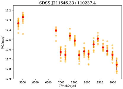
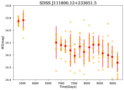
Figure 7: WISE and NEOWISE light curves at 3.4 $\mu$m of two of the luminosity declining AGN candidates, SDSS J211636.33+110237.4 (left) and SDSS J111800.12+233651.5 (right). Both light curves show a continuous flux decrease over the 10 yr long time span with $\Delta W1\sim 0.49$ mag (left) and $\Delta W1\sim 0.34$ mag (right), respectively.

3.4 Multi-Epoch SDSS Optical Spectra Spanning $1$–$10$ yr Time Gap

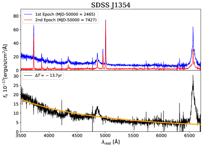
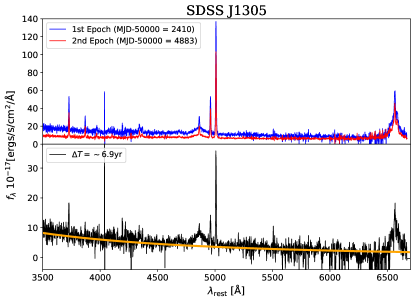
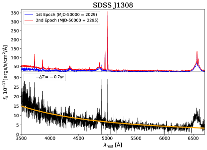
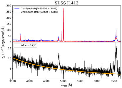
Figure 8: Top panels: The rest-frame optical spectra of the luminosity declining AGN candidates showing a changing-look behavior between the two epochs of the SDSS observations (the blue and red line represents the first and second epoch one, respectively). The observation dates are shown with the unit of MJD in the legend of each panel. Bottom panels: The subtracted spectrum between the two epoch (black) overlaid with the fitting curve of the theoretical accretion disk of $f_{\lambda}\propto\lambda^{2.3}$ (orange) (Shakura & Sunyaev, 1973).

The $\sim 10$ yr long IR variability by the WISE W1-band indicates that the luminosity declining AGN candidates tend to show large variabilities both in $\sim 10$ yr and $\sim 10^{3}$ yr. This motivates us to search the multi-epoch spectra given that our sample is obtained from the SDSS spectral surveys. We searched for multi-epoch spectra for our luminosity declining AGN candidates. Out of the 57 luminosity declining AGN candidates, 13 sources have the second epoch spectra observed in the later SDSS eBOSS survey (Abazajian et al., 2009; Dawson et al., 2013; Yanny et al., 2009; Dawson et al., 2016). The time difference between the first and second epoch spectra spans from $\sim$1 to 14 yr.

Considering that the fiber sizes are different between the SDSS BOSS (2 arcsec) and SDSS eBOSS (3 arcsec), the host galaxy continuum and the emission might contaminate strongly for the later SDSS eBOSS spectrum. On the other hand, this does not effect our study significantly, since our main motivation is to compare the central accretion disk components and the broad emission lines, both of which are considerably smaller than the current SDSS aperture sizes and their emission contributes equally to both of the spectra.

Based on the subtraction of the two-epoch spectra, we found four sources with a significant difference of the continuum and/or broad emission lines. Top panels of Figure 8 shows two AGN with a clear continuum and the broad component difference between the two epochs, so called changing-look (CL) AGN (LaMassa et al., 2015; MacLeod et al., 2016; Stern et al., 2018). SDSS J1354 shows a disappearance of the blue excess continuum associating the accretion disk emission and H$\beta$ broad component, and a weakened H$\alpha$ broad line, resulting a spectral type change from type-1 into type-1.9 (Osterbrock & Koski, 1976; Osterbrock, 1977, 1981). SDSS J1305 shows a disappearance of the blue excess continuum and a weakened H$\beta$, a spectral type change from type-1 into type-1.8. We also summarized the spectral properties in Table 2.

The bottom panels of Figure 8 shows two AGN with a significant continuum flux change (appearance for SDSS J1308 and disappearance for SDSS J1413) stronger than $3\sigma$ error of the associating continuum, but do not show a difference in broad emission components. We hereafter call those two sources as changing-look behavior (CLB) AGN to distinguish from the CL AGN with a clear sign of the flux changes of the broad emission.

The detection rate of CL AGN for our luminosity declining AGN candidates is extremely high reaching 15% ($2/13$), and even higher of 30% ($4/13$) if CLB AGN are included. This is a much more efficient pre-selection method by one to two orders of magnitude than the previous CL AGN searches, which have a range of detection rates from 0.4 to 1.3% after the pre-selections. For example, Potts & Villforth (2021) selected the candidates by applying the $\Delta g_{\mathrm{AB}}>0.16$, and found six sources out of the pre-selected 941 sources, whose success rate is $\sim 0.6$%. Yang et al. (2018) also utilized the SDSS multi-epoch spectra where one epoch is shown as a source category of “GALAXY”, but the other epoch shows a different category of “QSO” (or vice-versa). This method pre-selected 2023 candidates and 9 sources were genuinely CL sources, whose success rate is $\sim 0.4$%. The highest success rate was obtained through the study by MacLeod et al. (2016), who selected the candidates by applying the multi-epoch optical magnitude difference of $|\Delta g_{\mathrm{AB}}|>1$ mag with good signal-to-noise of $\sigma_{g}<0.15$ mag. This method selected 1011 candidates and 10 sources were CL AGN, and resulting success rate is 1.0%. This indicates that the long-term variability selection used in our study turn out to be an efficient method to search CL AGN tracing the variabilities in $\sim 10$ yr timescale.

Figure 9 shows the ALLWISE and NEOWISE light curves of the newly discovered four CL and CLB AGN. The black and gray solid vertical lines in each panel represent the observed MJD of the SDSS spectra, respectively. The black and gray dashed vertical lines represent the expected arrival time of the AGN activity seen in the SDSS spectra at the emitting region of the WISE W1-band emission by considering the time delays between the accretion disk and WISE W1-band. To estimate the light travel time from the center to the emitting region of the W1-band, we utilize the relation of Barvainis (1987) with the additional $k$-correction as following;

$$D_{\mathrm{sub}}/\mathrm{pc}=1.3\left(\dfrac{L_{\mathrm{bol,AD}}}{10^{46}\mathrm{~{}erg~{}s}^{-1}}\right)^{0.5}\left(\dfrac{T(1+z)}{1,500\mathrm{K}}\right)^{-2.8}$$ (5)

where we assume the emitted blackbody emission produced by the dust temperature of $T=850$K were detected in the WISE W1-band.

Those observing epochs of SDSS spectra as shown in Figure 9 give a sign that, for SDSS J1413, the second epoch of the SDSS spectra was taken at the faintest phase of the light-curve in the NEOWISE, which is consistent with the “disappearing” sign in the SDSS spectra. In addition, the current NEOWISE light-curve already reaches the same flux level as the ALLWISE fluxes which are close to the first epoch of the SDSS spectra, suggesting that the current optical spectra might show appearing feature again. For SDSS J1308 which shows an appearing feature, even though the two spectra are taken well before the ALLWISE light-curve range, the burst or bright-end phase might last until the current epoch.

Table 2: Basic information about the four new found CL and CLB AGN.

Name	SDSS OBJID DR7	Ra [°]	Dec [°]	$z$	Changing-look feature	Type
SDSS J135415.53+515925.7	587733410444607498	208.56	51.99	0.32	turning off	CL
SDSS J130501.41+604204.9	587732592255434858	196.26	60.70	0.38	turning off	CL
SDSS J130842.24+021924.4	587726015076433951	197.18	2.32	0.14	turning on	CLB
SDSS J141324.21+493424.9	588017713123557439	213.35	49.57	0.37	turning off	CLB

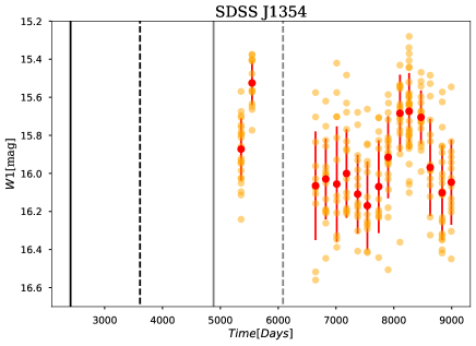
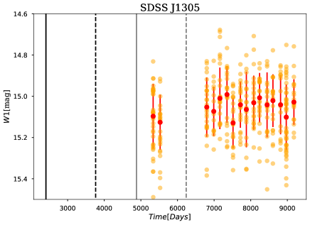
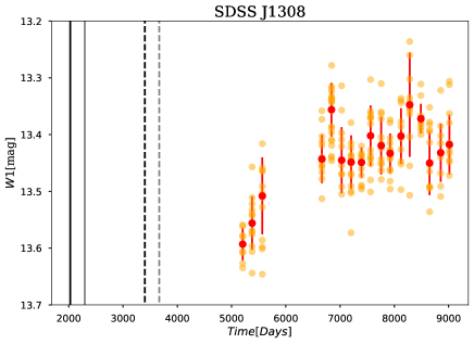
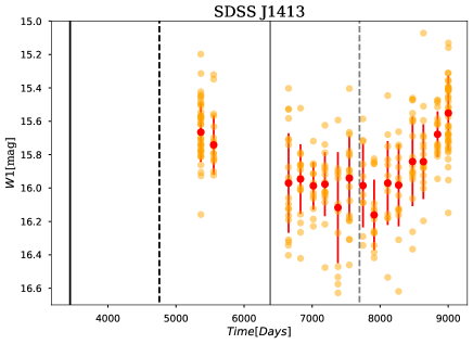
Figure 9: 3.4 $\mu$m WISE+NEOWISE light curve of the four CL and CLB AGN. The orange filled circle represents the obtained W1 magnitude at a given observing time. The red filled circle with errorbar represents the binned W1 magnitude at each epoch. The vertical straight lines represent the observing date of the obtained SDSS spectra. The black/gray one represents the date of the first/second epoch spectrum, respectively. The dashed lines represent the time of the arrival of the information of the accretion disk into the dusty torus region traced by the W1-band.

Sheng et al. (2017) showed that CL AGN show higher variabilities in the NEOWISE W1-band with $\Delta\mathrm{W1}>0.4$ mag, which is consistent with the cases of SDSS J1354 and the CLB AGN SDSS J1413 with $\Delta\mathrm{W1}=0.65$ and $\Delta\mathrm{W1}=0.61$ mag, respectively. On the other hand, the NEOWISE and the SDSS two epoch spectra do not simultaneously cover the transient phase of CL AGN for the remaining CL AGN and CLB AGN, and actually, they show smaller W1 variabilities of $\Delta\mathrm{W1}=0.14$ for J1305 and $\Delta\mathrm{W1}=0.25$ for J1308, respectively. This result indicates that the combination of the SDSS two epoch spectra and WISE variability further increases the probability to find such CL AGN by expanding the variability timespan by a factor of $\sim 2$ ($\sim 7000$ days).

3.5 Location of luminosity declining AGN candidates in the BPT Diagram

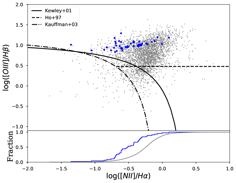
Figure 10: (Top): The distribution of luminosity declining AGN candidates (blue points) and parent sample (gray points) in the BPT diagram (Baldwin et al., 1981). The two sequences are shown separating the AGN and starforming galaxies (Kewley et al., 2001; Kauffmann et al., 2003) and the horizontal line separating the AGN and the LINERs (Ho et al., 1997). Bottom panel: Cumulative histogram of the line flux ratio of log([N ii]$\lambda 6584$/H$\alpha$).

Figure 10 shows the location of our luminosity declining AGN candidates (blue circles) and the parent type-1 AGN sources (gray dots) in the BPT diagram plane. Here, we limit our AGN to the additional SN cut for the emission lines, with SN$>=5$ for the narrow H$\alpha$, H$\beta$ , and [N ii]$\lambda 6584$ components, which are necessary for the sources to plot in the BPT diagram. This reduces the sample into 44 luminosity declining AGN candidates and 3042 parent sources.

Figure 10 demonstrates two important features of luminosity declining AGN candidates. One is that luminosity declining AGN candidates preferentially have higher $\log(\mathrm{[OIII]/H\beta})$ ratio with $\log(\mathrm{[OIII]/H\beta})\gtrsim 1.0$, which is likely originated from our selection criteria, requiring high observed [O iii]$\lambda 5007$  luminosity with $\log L_{\rm bol,[OIII]obs}>10^{45}$ erg s^-1 as shown in Figure 3.

The second is that luminosity declining AGN candidates are located wider range of log([N ii]$\lambda 6584$/H$\alpha$), spanning with $-1.5<$log([N ii]$\lambda 6584$/H$\alpha$)$<0$, but is located preferentially in the low ratio of log([N ii]$\lambda 6584$/H$\alpha$) $<-0.5$. The median ratio of log([N ii]$\lambda 6584$/H$\alpha$) is $-0.52\pm 0.27$ for the luminosity declining AGN candidates and $-0.24\pm 0.27$ for the parent sample. The cumulative histogram in the bottom panel of Figure 10 shows a notable difference between the two populations, with the $p$-value of $\sim 2\times 10^{-8}$, showing a significant distribution difference.

Groves et al. (2006) showed that the line flux ratio of log([N ii]$\lambda 6584$/H$\alpha$) depends strongly on the NLR gas metallicity and Kawasaki et al. (2017) also demonstrated that such low log([N ii]$\lambda 6584$/H$\alpha$) ratio with log([N ii]$\lambda 6584$/H$\alpha$)$=-1$–$-0.5$ cannot be described by the high ionization parameter alone, which is estimated from the oxygen line ratio diagrams of [O iii]$\lambda 5007$/[O iii]$\lambda 3727$ and [O i]$\lambda 6300$/[O iii]$\lambda 5007$. They defined a low-metallicity AGN if the sources have a flux ratio of log([N ii]$\lambda 6584$/H$\alpha$)$=-1$–$-0.5$, because the nitrogen relative abundance is in proportion to the metallicity, and roughly half of the luminosity declining AGN candidates fulfill such criterion. This suggests that some of our luminosity declining AGN candidates might be in an early chemical metal enrichment phase of galaxies (Kawasaki et al., 2017).

Kawasaki et al. (2017) defined a “BPT-valley” AGN, which are selected based on the region above the sequence of Kauffmann et al. (2003) (black solid curve) and the low Nitrogen abundance of log([N ii]$\lambda 6584$/ H$\alpha$) $<-0.5$. They found that a significant fraction of these selected AGN show low metallicity features. We followed the same manner of Kawasaki et al. (2017) to select these BPT valley sources from our parent type-1 AGN sample, which leaves 721 objects. To investigate whether BPT valley sources have a similar variability feature as shown in our luminosity declining AGN candidates, we also calculate the $\log(R)$ and $\Delta$W1 for the BPT valley population in our sample. The BPT valley population shows $\log(R)=-0.32\pm 0.40$, which is slightly lower than the value of the parent sample of $\log(R)=-0.02\pm 0.37$ and their significance is statistically significant with the $p$-value of $\sim 10^{-16}$. Our luminosity declining AGN candidates show lower $\log(R)$ of $-1.07\pm 0.09$ and therefore also the p-value of the distribution difference between the luminosity decline AGN candidates and the BPT valley population is $\sim 10^{-16}$. Thus, BPT valley population and luminosity decline AGN is essentially the different population in terms of the obtained $R$ values. That is, a low-metallicity environment alone cannot reproduce a such significant AGN luminosity decline.

The WISE variability is $\Delta W_{1}=0.39$ for the BPT valley population, which is between the luminosity declining AGN candidates ($\Delta W_{1}=0.41$) and the parent sample ($\Delta W_{1}=0.36$). The BPT valley and the parent sample show a different distribution for the variability this is also suggested by the $p$-value of 0.02, but show a similar one to our luminosity declining AGN candidates with the $p$-value of 0.6.

It is naively expected that the stellar mass of low-metallicity AGN would reside in a relatively low stellar-mass galaxies, i.e., $M_{\star}<10^{10}M_{\odot}$, as shown in star-forming galaxies at each cosmic epoch (e.g., Tremonti et al., 2004; Lee et al., 2006; Erb et al., 2006). In addition, some studies suggest that AGN in low stellar-mass galaxies tend to show a higher AGN variability amplitude in the optical bands (e.g., Kimura et al., 2020; Burke et al., 2021), while some report that mass dependence is weak (Caplar et al., 2017). On the other hand, it is not still clear whether low-metallicity AGN reside in low-stellar mass galaxies. Considering that our sample is type-1 AGN, the stellar-mass is hard to be constrained with the current sample set. Instead, we compare the BH mass distributions of each subgroup as an indicator of the stellar-mass which is inferred from the scaling relation between $M_{\rm BH}$ and $M_{\star}$ (e.g., Kormendy & Ho, 2013). The median $M_{\rm BH}$ of each subgroup is $\left<\log(M_{\mathrm{BH}}/M_{\odot})\right>=8.0$, $7.8$, and $7.8$ for luminosity declining AGN candidates, BPT-valley AGN, and the parent sample, respectively. Assuming the relation between $M_{\rm BH}$ and $M_{\star}$ of Kormendy & Ho (2013), the expected stellar-mass is $\left<\log(M_{\star}/M_{\odot})\right>=10.3$, $10.2$, and $10.2$, respectively. This suggests that most of luminosity declining AGN candidates do not reside in low-stellar mass galaxies with $M_{\star}<10^{10}M_{\odot}$, but hey reside in relatively massive ones. The BPT valley AGN also show similar trend and this relatively massive stellar-mass of the host galaxies with $M_{\star}>10^{10}M_{\odot}$ is consistent with the result of Kawasaki et al. (2017). One possible mechanism of such low metallicity AGN in the relatively massive host galaxies can be realized if the inflow of the low metallicity gas occurs from the IGM and/or surrounding environment (Husemann et al., 2011).

4 Discussion

4.1 How long does super-Eddington phase last?

Our study shows that there are variable AGN in the time span of $10^{3-4}$ yr, and their AGN luminosities used to reach around the Eddington limit. This suggests that the lifetime of such burst phase around the Eddington limit ($t_{\mathrm{burst}}$) may not last long, a timescale of $10^{3-4}$ yr. Since the Eddington ratio is estimated for all sample in this study at the three epochs as shown in Figure 5, we here estimate $t_{\mathrm{burst}}$ from the number fraction of such super-Eddington phase at each epoch.

We first count the number of sources above the Eddington limit at each AGN indicator, $N_{i,\mathrm{Edd}}$ (where $i=$NLR, torus or AD), and if the sources are above the Eddington limit in the two epoch, those numbers are written as $N_{i+j,\mathrm{Edd}}$, where $i,j=$NLR, torus, and AD and $D_{i}>D_{j}$. Since the $\lambda_{\mathrm{Edd}}$ has a certain error, we treat the source as super-Eddington sources only when the $\lambda_{\mathrm{Edd}}-3\Delta\lambda_{\mathrm{Edd}}>1$. Then we calculate the number fraction which are beyond the Eddington both in the torus and NLR indicators, and the obtained fraction is $f_{\mathrm{Edd}}=N_{\mathrm{NLR+torus,Edd}}/N_{\mathrm{NLR,Edd}}=15/114=0.13$. We assume that the burst phase lasts with a stable luminosity for the timespan of $t_{\mathrm{burst}}$. In this case, $f_{\mathrm{Edd}}$ depends on the $t_{\mathrm{burst}}$ phase as following

$$f_{\mathrm{Edd}}=\exp\left(-\dfrac{\Delta t}{t_{\mathrm{burst}}}\right),$$ (6)

where $\Delta t$ is the lookback time difference between the torus and NLR, and essentially it is dominated by the look back time to the NLR, with $\Delta t\sim 10^{3.8\pm 0.1}$ yr (see Figure 5). Thus, $t_{\mathrm{burst}}=-\Delta t/\log(f_{\mathrm{Edd}})\simeq 10^{3.5}$ yr . This is four-to-five orders of magnitude shorter than the total lifetime of AGN of $\sim 10^{8}$ yr (Marconi et al., 2004), and even one to two orders of magnitude shorter than the typical one-cycle ($t_{\mathrm{AGN}}$) AGN lifetime of $10^{5}$ yr (Schawinski et al., 2015). Therefore, super-Eddington phase can be achieved a certain fraction of the AGN lifetime of $f_{\mathrm{burst,Edd}}=t_{\mathrm{burst}}/t_{\mathrm{AGN}}\sim 0.01$–$0.1$.

Although $f_{\mathrm{burst,Edd}}$ is small and our sample is based on low-$z$ high-luminosity type-1 AGN in the low-$z$ universe at $z<0.4$, the suggested $f_{\mathrm{burst,Edd}}\sim 0.1$ might alleviate the current challenge to the quasar evolution is seen in $z>6$, where most of the luminous quasars require the Eddington-limit accretion with the duty cycle of nearly one (Willott et al., 2010; Mortlock et al., 2011; Wu et al., 2015; Bañados et al., 2018; Wang et al., 2021; Yang et al., 2021). Assuming that the luminous quasars experience a super-Eddington phase with 10% of their quasar lifetime, and the accretion rate can exceed the Eddington limit by a factor of up to $\sim 10$–$100$ (Ohsuga et al., 2005; Jiang et al., 2014; Sadowski et al., 2015; Inayoshi et al., 2016, 2020), which reduces the required quasar growth time by a factor of 2–10.

Recently, the lifetime of high-$z$ ($z>6$) quasars have been reported through the measurements of the physical extents of hydrogen Ly$\alpha$ proximity zones (Davies et al., 2020; Eilers et al., 2018, 2021). Some sources show a small physical size, and therefore the inferred quasar lifetime is substantially short, with the order of $10^{3-4}$ yr. Given that the inferred quasar lifetimes of such $z>6$ quasars are substantially shorter than the e-folding timescale of the Eddington-limited accretion with $t_{\mathrm{Edd}}\simeq 4.5\times 10^{6}$ yr, Inayoshi et al. (2021) suggested that those quasars are expected to experience the super-Eddington accretion phase to grow up. This short timescale of $10^{3-4}$ yr is consistent with our expected $t_{\mathrm{burst}}$ of the super-Eddingon phase of local AGN at $z<0.4$. This might be a coincidence, but it is seen in both quasars at $z>6$ and $z<0.4$. If a constant $t_{\mathrm{burst}}\sim 0.1$ of the super-Eddington phase is ubiquitously seen across the cosmic epoch, the lifetime of such super-Eddington phase would be fundamentally governed by the BH accretion disk physics and unrelated to the cosmological environment once enough gas supply is achieved into the central engine.

4.2 What are luminosity declining AGN candidates in this study?

Our goal is to search for luminosity declining AGN who has experienced a large flux decline in the past $10^{3-4}$ yrs, and we selected 57 [O iii]$\lambda 5007$ bright and MIR faint AGN as luminosity declining AGN candidates. Figure 5 exhibits that our method selects sources that experienced burst phase reaching the Eddington limit, and rapidly declined AGN luminosities at least by a factor of 10 in the last $10^{3-4}$ yr.

In addition to such feature in the longterm flux change of $\sim 10^{3-4}$ yr span, a certain fraction of such luminosity declining AGN candidates also show variabilities even in the last $\sim 10$ yr scale, which has been supported from the NEOWISE light curve and the SDSS multi-epoch spectra with high cadence of the changing-look AGN feature. This suggests that our method turn out to be an efficient way to select not only for a long-term AGN variability of $\sim 10^{3-4}$ yr, but also for a relatively shorter-term AGN variability with $<10$ yr timescale.

Several authors have already discussed that the flux change of $\sim 10$ yr timescale, notably for changing-look AGN, has a different physical origin from the one shown in fading AGN with $\sim 10^{3-4}$ yr timescale. The latter timescale is roughly consistent with the viscous timescale, an inflow timescale of the gas accretion, and can be realized once rapid accretion rate change occurs in the accretion disk (e.g., see discussions in Ichikawa et al., 2019a, b). It was discussed that the origin of the flux change in the timespan of $\sim$yr to $\sim 10$ yr rather originates from the instability of the accretion disk (LaMassa et al., 2015; Ruan et al., 2016; MacLeod et al., 2016; Stern et al., 2018).

One key insight obtained from this study is that the two epoch spectra are obtained with the timespan of 1–14 yr, and the average BH mass of the sample is $\left<M_{\rm BH}\right>\sim 10^{8}$ $M_{\odot}$. This suggests that the observed changing-look behavior should occur within $\sim 10$ yr in the system of $\left<M_{\rm BH}\right>\sim 10^{8}$ $M_{\odot}$. This can rule out some disk timescales as origins of the changing-look behavior. For example, the heating and cooling fronts propagation instability in the disk occurs in the timescale of $t_{\mathrm{front}}\sim 20(M_{\rm BH}/10^{8}M_{\odot})$ yr by assuming that the scale height of the disk is $h/R=0.05$, the disk viscous parameter of $\alpha=0.03$. Since our observing epoch covers the time span of 14 yr at the maximum, the characteristic cooling front timescale might match with the changing-look events shown in our sources. On the other hand, the thermal timescale of the disk, which can be written as $t_{\mathrm{th}}\sim 1\times(M_{\rm BH}/10^{8}M_{\odot})$ year, is slightly too short.

Noda & Done (2018) discussed such changing-look AGN behavior is tightly connected to the state change and such change preferentially occurs at a specific Eddington ratio range of around $\log\lambda\sim-1$ to $-1.5$ and a timescale of several years. Considering that most of our luminosity declining AGN candidates have Eddington ratio of around this range and their timescales are also consistent with the expectation from Noda & Done (2018), this might be related to such state change and our sample might preferentially pick up changing-look AGN with the association of the state change.

In summary, the origins of the possible connection of the luminosity change between the 10 yr timescale and $10^{3-4}$ yr are still uncertain, but the preference of the changing-look behavior at the specific Eddington ratio of $\log\lambda_{\mathrm{Edd}}\sim-1$ to $-1.5$ and the $\sim 10^{3}$ yr long burst phase at the Eddington ratio of $\log\lambda_{\mathrm{Edd}}\sim 0$ suggests that both timescales might connect to the state transition events in the accretion disk. Although the current sample still limits the sample size to only 4 sources who experienced the variabilities both in 10 yr and $10^{3}$ yr, the incremental sample will happen soon once the eROSITA (Predehl et al., 2021) X-ray all-sky data become public at the beginning of 2023. eROSITA will provide the current AGN luminosity for our type-1 AGN sample without worrying about the dust or gas obscuration to the line of sight. Also, the 0.5–2 keV flux limit of eROSITA in the final integration of the planned four years program (eRASS8) in the ecliptic equatorial region ($f_{\mathrm{0.5-2keV}}=1.1\times 10^{-14}~{}$ erg s^-1 cm^-2 Predehl et al., 2021) is way deeper than the expected one estimated from the WISE W3 (12 $\mu$m) band flux density limit, where $f_{\nu,\mathrm{lim}}=1$ mJy corresponds to $f_{\mathrm{0.5-2keV}}=8.3\times 10^{-14}$ erg s^-1 cm^-2, by assuming the local X-ray–MIR luminosity correlation of AGN (Gandhi et al., 2009b; Asmus et al., 2015; Ichikawa et al., 2012, 2017).

4.3 Radio Properties of Luminosity Declining AGN

We here discuss the radio properties of the luminosity declining AGN since most of the [O iii]$\lambda 5007$ luminous extremely red quasars at $z\sim 2$–$3$ (Ross et al., 2015; Hamann et al., 2017) are known to be radio bright sources with $\nu L_{\mathrm{1.4GHz}}\simeq 10^{40-41}$ erg s^-1 (e.g., Zakamska & Greene, 2014; Hwang et al., 2018), which likely originate from shocks caused by wide-angle quasar winds, and it is worth to check whehter our sources could be local ($z<0.4$) analogous to them.

Mullaney et al. (2013) summarized the radio properties of our parent sample based on the 1.4 GHz radio detections by the VLA/FIRST (Becker et al., 1995; White et al., 1997; Helfand et al., 2015) and NVSS (Condon et al., 1998) surveys at a limiting flux density of $>2$ mJy, by following the similar manner of Best et al. (2005). Out of our 57 luminosity declining AGN candidates, 7 sources have such radio detections with the median radio luminosity of $L_{\mathrm{1.4GHz}}\simeq 10^{24}$ W Hz^-1 or $\nu L_{\mathrm{1.4GHz}}\simeq 10^{40}$ erg s^-1, whose radio to bolometric luminosity ratio is $\log(\nu L_{\mathrm{1.4GHz}}/L_{\rm bol,[OIII]obs})\simeq-6.2$, which is comparable with the value expected from the quasar wind scenario (e.g., Hwang et al., 2018).

The radio detection rate of luminosity declining AGN is $7/57\simeq 0.12$, which is slightly higher than that of our parent sample of $460/7653\simeq 0.06$, and is closer to the detection rate of the extremely red quasars of $9/97\simeq 0.09$ at a same radio survey depth. Although the sample size is too small at this stage, such higher radio detection rate might be a result of the enhancement of the radio emission by the shocks from the AGN radio driven outflow, as discussed in Zakamska & Greene (2014). If our luminosity declining AGN are in the similar population of extremely red quasar at $z=2$–$3$, luminosity declining AGN are also likely in the act of the strong AGN feedback phase with a strong radiative outflow, and this scenario is also consistent with the experience of the AGN luminosity declining over the past $10^{3-4}$ yr, partially because of the shortage supply of the gas into the nucleus. However, we also note that the additional deeper radio observations are necessary to confirm that the similar radio properties can be obtained for the remaining FIRST or NVSS non-detected luminosity declining AGN.

Some might also wonder that blazars might contaminate the sample of luminosity declining AGN. For the 7 radio detected sources in our sample, their optical spectra are dominated by the strong emission lines as well as the blue continuum, which is a natural outcome based on our selection criteria of type-1 AGN with strong [O iii]$\lambda 5007$ emission lines with the signal-to-noise ratio of S/N$\geq 5$. This rules out a possibility that they are BL Lac sources whose optical continuum should not show any emission lines. In addition, their 1.4 GHz radio luminosity is around $\nu L_{\mathrm{1.4GHz}}\sim 10^{40}$ erg s^-1. This is at least one order of magnitude fainter than the typical observed radio luminosity range of the flat spectrum radio quasars (e.g., Ghisellini et al., 2017). Based on those results, we conclude that blazar contamination is unlikely for our 7 radio detected luminosity declining AGN.

5 Conclusion

We systematically search for an AGN population who has experienced a significant AGN luminosity decline in the past $10^{3-4}$ yr by utilizing the advantage of the difference of the physical size of each AGN indictor, spanning from $<1$ pc to $\gtrsim 1$ kpc. We cross-matched the $\sim 7,700$ SDSS DR7 type-1 AGN at $z<0.4$ (Mullaney et al., 2011), covering the [O iii]$\lambda 5007$ emission line which is a tracer for the $\sim$kpc scale narrow-line region (NLR) emission, with the WISE IR catalog which traces the AGN dust emission in the central $\sim 10$ pc scale. With our selection of at least one magnitude fainter in the AGN dust luminosity than the one from the NLR, we selected an interesting population of the luminosity declining AGN candidates who has experienced the AGN luminosity decrease by a factor of $>10$ in the previous $10^{3-4}$ yr. The sample contains 57 AGN and our results show interesting properties which give key insights to the BH and accretion disk physics as written below.

1. The parent type-1 AGN sample shows on average the constant Eddington ratio over the previous $10^{3-4}$ yr, indicating that the intrinsic AGN variability within $\sim 10^{3-4}$ yr should be on average smaller than the scatter of 0.4 dex. On the other hand, the luminosity decline AGN candidates show a large luminosity decline in the previous $10^{3-4}$ yr and their previous AGN luminosities reached almost Eddington limit of $\log\lambda_{\mathrm{Edd}}\sim 0$, while the current Eddington ratio is almost similar with those of the parent sample of $\lambda_{\mathrm{Edd}}\sim-1.5$, indicating the drastic luminosity decline by a factor of $>10$.

2. Utilizing the 3.4 $\mu$m light-curves obtained from ALLWISE and NEOWISE, the luminosity decline AGN candidates show a relatively larger W1-band variability of 0.41 compared to the parent sample of 0.35. In addition, two sources show a continuous flux decline over $\sim 10$ yr, suggesting that at least two sources still experience the luminosity decline in the last 10 yr, a possible continuous flux decrease over $10^{4}$ yr.

3. Thirteen out of the 57 luminosity declining AGN candidates have multi-epoch SDSS spectra and two out of them show a spectral type change associating with a disappearing continuum and broad line emissions, which is so called a changing-look phenomenon. The finding rate is $15$%, which is two to three orders of magnitude higher than the random selection of the changing-look AGN. Combined with the higher IR varibility signature in the WISE bands, our method to select variability AGN in the past $10^{3-4}$ yr might also be an efficient method to select AGN who has recently experienced the AGN variability in the past $\sim 10$ yr.

4. The location of the luminosity declining AGN candidates in the BPT-diagram is different from the the parent type-1 AGN sample, notably a lower median flux ratio of $\log$([N ii]$\lambda 6584/\mathrm{H}\alpha\lambda 6563)=-0.52$ than $\log$([N ii]$\lambda 6584/\mathrm{H}\alpha\lambda 6563)=-0.24$ for the parent sample. Considering that the lower flux ratio indicates that their NLR gas has a lower gas metallicity, luminosity declining AGN candidates might prefer the host galaxies with younger and gas rich host galaxies, resulting the past AGN burst reaching the Eddington limit accretion.

5. Utilizing this long-term light-curve, we estimate the lifetime of the burst phase realizing the super-Eddington accretion. The estimated lifetime is $t_{\mathrm{burst}}\simeq 10^{3.5}$ yr, suggesting that the super-Eddington phase can be achieved only in a certain fraction of the AGN lifetime of $t_{\mathrm{burst}}/t_{\mathrm{AGN}}\sim 0.01$–$0.1$.

References

- Abazajian et al. (2009) Abazajian, K. N., Adelman-McCarthy, J. K., Agüeros, M. A., et al. 2009, ApJS, 182, 543, doi: 10.1088/0067-0049/182/2/543
- Alonso-Herrero et al. (2011) Alonso-Herrero, A., Ramos Almeida, C., Mason, R., et al. 2011, ApJ, 736, 82, doi: 10.1088/0004-637X/736/2/82
- Antonucci (1993) Antonucci, R. 1993, ARA&A, 31, 473, doi: 10.1146/annurev.aa.31.090193.002353
- Asmus et al. (2015) Asmus, D., Gandhi, P., Hönig, S. F., Smette, A., & Duschl, W. J. 2015, MNRAS, 454, 766, doi: 10.1093/mnras/stv1950
- Assef et al. (2018) Assef, R. J., Stern, D., Noirot, G., et al. 2018, ApJS, 234, 23, doi: 10.3847/1538-4365/aaa00a
- Astropy Collaboration et al. (2018) Astropy Collaboration, Price-Whelan, A. M., Sipőcz, B. M., et al. 2018, AJ, 156, 123, doi: 10.3847/1538-3881/aabc4f
- Bañados et al. (2018) Bañados, E., Venemans, B. P., Mazzucchelli, C., et al. 2018, Nature, 553, 473, doi: 10.1038/nature25180
- Bae et al. (2017) Bae, H.-J., Woo, J.-H., Karouzos, M., et al. 2017, ApJ, 837, 91, doi: 10.3847/1538-4357/aa5f5c
- Baldwin et al. (1981) Baldwin, J. A., Phillips, M. M., & Terlevich, R. 1981, PASP, 93, 5, doi: 10.1086/130766
- Barvainis (1987) Barvainis, R. 1987, ApJ, 320, 537, doi: 10.1086/165571
- Becker et al. (1995) Becker, R. H., White, R. L., & Helfand, D. J. 1995, ApJ, 450, 559, doi: 10.1086/176166
- Bennert et al. (2002) Bennert, N., Falcke, H., Schulz, H., Wilson, A. S., & Wills, B. J. 2002, ApJ, 574, L105, doi: 10.1086/342420
- Berney et al. (2015) Berney, S., Koss, M., Trakhtenbrot, B., et al. 2015, MNRAS, 454, 3622, doi: 10.1093/mnras/stv2181
- Best et al. (2005) Best, P. N., Kauffmann, G., Heckman, T. M., et al. 2005, MNRAS, 362, 25, doi: 10.1111/j.1365-2966.2005.09192.x
- Burke et al. (2021) Burke, C. J., Liu, X., Shen, Y., et al. 2021, arXiv e-prints, arXiv:2111.03079. https://arxiv.org/abs/2111.03079
- Burtscher et al. (2013) Burtscher, L., Meisenheimer, K., Tristram, K. R. W., et al. 2013, A&A, 558, A149, doi: 10.1051/0004-6361/201321890
- Calzetti et al. (2000) Calzetti, D., Armus, L., Bohlin, R. C., et al. 2000, ApJ, 533, 682, doi: 10.1086/308692
- Caplar et al. (2017) Caplar, N., Lilly, S. J., & Trakhtenbrot, B. 2017, ApJ, 834, 111, doi: 10.3847/1538-4357/834/2/111
- Cardelli et al. (1989) Cardelli, J. A., Clayton, G. C., & Mathis, J. S. 1989, ApJ, 345, 245, doi: 10.1086/167900
- Chen et al. (2019) Chen, X., Akiyama, M., Noda, H., et al. 2019, PASJ, 71, 29, doi: 10.1093/pasj/psz002
- Chen et al. (2020a) Chen, X., Ichikawa, K., Noda, H., et al. 2020a, ApJ, 905, L2, doi: 10.3847/2041-8213/abca30
- Chen et al. (2020b) Chen, X., Akiyama, M., Ichikawa, K., et al. 2020b, ApJ, 900, 51, doi: 10.3847/1538-4357/aba599
- Condon et al. (1998) Condon, J. J., Cotton, W. D., Greisen, E. W., et al. 1998, AJ, 115, 1693, doi: 10.1086/300337
- Cutri et al. (2013) Cutri, R. M., Wright, E. L., Conrow, T., et al. 2013, Explanatory Supplement to the AllWISE Data Release Products, Explanatory Supplement to the AllWISE Data Release Products
- Dai et al. (2010) Dai, X., Kochanek, C. S., Chartas, G., et al. 2010, ApJ, 709, 278, doi: 10.1088/0004-637X/709/1/278
- Davies et al. (2020) Davies, F. B., Hennawi, J. F., & Eilers, A.-C. 2020, MNRAS, 493, 1330, doi: 10.1093/mnras/stz3303
- Dawson et al. (2013) Dawson, K. S., Schlegel, D. J., Ahn, C. P., et al. 2013, AJ, 145, 10, doi: 10.1088/0004-6256/145/1/10
- Dawson et al. (2016) Dawson, K. S., Kneib, J.-P., Percival, W. J., et al. 2016, AJ, 151, 44, doi: 10.3847/0004-6256/151/2/44
- Domínguez et al. (2013) Domínguez, A., Siana, B., Henry, A. L., et al. 2013, ApJ, 763, 145, doi: 10.1088/0004-637X/763/2/145
- Eilers et al. (2018) Eilers, A.-C., Hennawi, J. F., & Davies, F. B. 2018, ApJ, 867, 30, doi: 10.3847/1538-4357/aae081
- Eilers et al. (2021) Eilers, A.-C., Hennawi, J. F., Davies, F. B., & Simcoe, R. A. 2021, ApJ, 917, 38, doi: 10.3847/1538-4357/ac0a76
- Erb et al. (2006) Erb, D. K., Shapley, A. E., Pettini, M., et al. 2006, ApJ, 644, 813, doi: 10.1086/503623
- Esparza-Arredondo et al. (2020) Esparza-Arredondo, D., Osorio-Clavijo, N., González-Martín, O., et al. 2020, ApJ, 905, 29, doi: 10.3847/1538-4357/abc425
- Gandhi et al. (2009a) Gandhi, P., Horst, H., Smette, A., et al. 2009a, A&A, 502, 457, doi: 10.1051/0004-6361/200811368
- Gandhi et al. (2009b) —. 2009b, A&A, 502, 457, doi: 10.1051/0004-6361/200811368
- Ghisellini et al. (2017) Ghisellini, G., Righi, C., Costamante, L., & Tavecchio, F. 2017, MNRAS, 469, 255, doi: 10.1093/mnras/stx806
- Greene & Ho (2005) Greene, J. E., & Ho, L. C. 2005, ApJ, 630, 122, doi: 10.1086/431897
- Greenland et al. (2016) Greenland, S., Senn, S. J., Rothman, K. J., et al. 2016, European journal of epidemiology, 31, 337
- Groves et al. (2006) Groves, B., Dopita, M., & Sutherland, R. 2006, A&A, 458, 405, doi: 10.1051/0004-6361:20065097
- Hainline et al. (2013) Hainline, K. N., Hickox, R., Greene, J. E., Myers, A. D., & Zakamska, N. L. 2013, ApJ, 774, 145, doi: 10.1088/0004-637X/774/2/145
- Hamann et al. (2017) Hamann, F., Zakamska, N. L., Ross, N., et al. 2017, MNRAS, 464, 3431, doi: 10.1093/mnras/stw2387
- Heckman et al. (2004) Heckman, T. M., Kauffmann, G., Brinchmann, J., et al. 2004, ApJ, 613, 109, doi: 10.1086/422872
- Helfand et al. (2015) Helfand, D. J., White, R. L., & Becker, R. H. 2015, ApJ, 801, 26, doi: 10.1088/0004-637X/801/1/26
- Ho et al. (1997) Ho, L. C., Filippenko, A. V., & Sargent, W. L. W. 1997, ApJS, 112, 315, doi: 10.1086/313041
- Hönig et al. (2012) Hönig, S. F., Kishimoto, M., Antonucci, R., et al. 2012, ApJ, 755, 149, doi: 10.1088/0004-637X/755/2/149
- Hönig et al. (2013) Hönig, S. F., Kishimoto, M., Tristram, K. R. W., et al. 2013, ApJ, 771, 87, doi: 10.1088/0004-637X/771/2/87
- Hook et al. (1994) Hook, I. M., McMahon, R. G., Boyle, B. J., & Irwin, M. J. 1994, MNRAS, 268, 305, doi: 10.1093/mnras/268.2.305
- Hopkins et al. (2006) Hopkins, P. F., Hernquist, L., Cox, T. J., et al. 2006, ApJS, 163, 1, doi: 10.1086/499298
- Hopkins et al. (2007) Hopkins, P. F., Richards, G. T., & Hernquist, L. 2007, ApJ, 654, 731, doi: 10.1086/509629
- Hunter (2007) Hunter, J. D. 2007, Computing in Science & Engineering, 9, 90, doi: 10.1109/MCSE.2007.55
- Husemann et al. (2014) Husemann, B., Jahnke, K., Sánchez, S. F., et al. 2014, MNRAS, 443, 755, doi: 10.1093/mnras/stu1167
- Husemann et al. (2011) Husemann, B., Wisotzki, L., Jahnke, K., & Sánchez, S. F. 2011, A&A, 535, A72, doi: 10.1051/0004-6361/201117596
- Hwang et al. (2018) Hwang, H.-C., Zakamska, N. L., Alexandroff, R. M., et al. 2018, MNRAS, 477, 830, doi: 10.1093/mnras/sty742
- Ichikawa et al. (2017) Ichikawa, K., Ricci, C., Ueda, Y., et al. 2017, ApJ, 835, 74, doi: 10.3847/1538-4357/835/1/74
- Ichikawa & Tazaki (2017a) Ichikawa, K., & Tazaki, R. 2017a, ApJ, 844, 21, doi: 10.3847/1538-4357/aa7891
- Ichikawa & Tazaki (2017b) —. 2017b, ApJ, 844, 21, doi: 10.3847/1538-4357/aa7891
- Ichikawa et al. (2019a) Ichikawa, K., Ueda, J., Bae, H.-J., et al. 2019a, ApJ, 870, 65, doi: 10.3847/1538-4357/aaf233
- Ichikawa et al. (2016) Ichikawa, K., Ueda, J., Shidatsu, M., Kawamuro, T., & Matsuoka, K. 2016, PASJ, 68, 9, doi: 10.1093/pasj/psv112
- Ichikawa et al. (2012) Ichikawa, K., Ueda, Y., Terashima, Y., et al. 2012, ApJ, 754, 45, doi: 10.1088/0004-637X/754/1/45
- Ichikawa et al. (2015) Ichikawa, K., Packham, C., Ramos Almeida, C., et al. 2015, ApJ, 803, 57, doi: 10.1088/0004-637X/803/2/57
- Ichikawa et al. (2019b) Ichikawa, K., Kawamuro, T., Shidatsu, M., et al. 2019b, ApJ, 883, L13, doi: 10.3847/2041-8213/ab3ebf
- Ichikawa et al. (2019c) Ichikawa, K., Ricci, C., Ueda, Y., et al. 2019c, ApJ, 870, 31, doi: 10.3847/1538-4357/aaef8f
- Inayoshi & Haiman (2016) Inayoshi, K., & Haiman, Z. 2016, ApJ, 828, 110, doi: 10.3847/0004-637X/828/2/110
- Inayoshi et al. (2016) Inayoshi, K., Haiman, Z., & Ostriker, J. P. 2016, MNRAS, 459, 3738, doi: 10.1093/mnras/stw836
- Inayoshi et al. (2021) Inayoshi, K., Nakatani, R., Toyouchi, D., et al. 2021, arXiv e-prints, arXiv:2110.10693. https://arxiv.org/abs/2110.10693
- Inayoshi et al. (2020) Inayoshi, K., Visbal, E., & Haiman, Z. 2020, ARA&A, 58, 27, doi: 10.1146/annurev-astro-120419-014455
- Jaffe et al. (2004) Jaffe, W., Meisenheimer, K., Röttgering, H. J. A., et al. 2004, Nature, 429, 47, doi: 10.1038/nature02531
- Jiang et al. (2014) Jiang, Y.-F., Stone, J. M., & Davis, S. W. 2014, ApJ, 796, 106, doi: 10.1088/0004-637X/796/2/106
- Kato et al. (2008) Kato, S., Fukue, J., & Mineshige, S. 2008, Black-Hole Accretion Disks — Towards a New Paradigm —
- Kauffmann et al. (2003) Kauffmann, G., Heckman, T. M., Tremonti, C., et al. 2003, MNRAS, 346, 1055, doi: 10.1111/j.1365-2966.2003.07154.x
- Kawamuro et al. (2017) Kawamuro, T., Schirmer, M., Turner, J. E. H., Davies, R. L., & Ichikawa, K. 2017, ApJ, 848, 42, doi: 10.3847/1538-4357/aa8e46
- Kawasaki et al. (2017) Kawasaki, K., Nagao, T., Toba, Y., Terao, K., & Matsuoka, K. 2017, ApJ, 842, 44, doi: 10.3847/1538-4357/aa70e1
- Keel et al. (2017) Keel, W. C., Lintott, C. J., Maksym, W. P., et al. 2017, ApJ, 835, 256, doi: 10.3847/1538-4357/835/2/256
- Kewley et al. (2001) Kewley, L. J., Dopita, M. A., Sutherland, R. S., Heisler, C. A., & Trevena, J. 2001, ApJ, 556, 121, doi: 10.1086/321545
- Kimura et al. (2020) Kimura, Y., Yamada, T., Kokubo, M., et al. 2020, ApJ, 894, 24, doi: 10.3847/1538-4357/ab83f3
- King (2016) King, A. 2016, MNRAS, 456, L109, doi: 10.1093/mnrasl/slv186
- Kishimoto et al. (2011) Kishimoto, M., Hönig, S. F., Antonucci, R., et al. 2011, A&A, 536, A78, doi: 10.1051/0004-6361/201117367
- Kormendy & Ho (2013) Kormendy, J., & Ho, L. C. 2013, ARA&A, 51, 511, doi: 10.1146/annurev-astro-082708-101811
- Koshida et al. (2014) Koshida, S., Minezaki, T., Yoshii, Y., et al. 2014, ApJ, 788, 159, doi: 10.1088/0004-637X/788/2/159
- Kozłowski et al. (2010) Kozłowski, S., Kochanek, C. S., Udalski, A., et al. 2010, ApJ, 708, 927, doi: 10.1088/0004-637X/708/2/927
- LaMassa et al. (2015) LaMassa, S. M., Cales, S., Moran, E. C., et al. 2015, ApJ, 800, 144, doi: 10.1088/0004-637X/800/2/144
- Lee et al. (2006) Lee, H., Skillman, E. D., Cannon, J. M., et al. 2006, ApJ, 647, 970, doi: 10.1086/505573
- López-Gonzaga et al. (2016) López-Gonzaga, N., Burtscher, L., Tristram, K. R. W., Meisenheimer, K., & Schartmann, M. 2016, A&A, 591, A47, doi: 10.1051/0004-6361/201527590
- Lopez-Rodriguez et al. (2018) Lopez-Rodriguez, E., Fuller, L., Alonso-Herrero, A., et al. 2018, ApJ, 859, 99, doi: 10.3847/1538-4357/aabd7b
- MacLeod et al. (2010) MacLeod, C. L., Ivezić, Ž., Kochanek, C. S., et al. 2010, ApJ, 721, 1014, doi: 10.1088/0004-637X/721/2/1014
- MacLeod et al. (2016) MacLeod, C. L., Ross, N. P., Lawrence, A., et al. 2016, MNRAS, 457, 389, doi: 10.1093/mnras/stv2997
- Mainzer (2014) Mainzer, A. 2014, NEOWISE-R Single Exposure (L1b) Source Table, IPAC, doi: 10.26131/IRSA144. https://catcopy.ipac.caltech.edu/dois/doi.php?id=10.26131/IRSA144
- Mainzer et al. (2011) Mainzer, A., Bauer, J., Grav, T., et al. 2011, ApJ, 731, 53, doi: 10.1088/0004-637X/731/1/53
- Mainzer et al. (2014) Mainzer, A., Bauer, J., Cutri, R. M., et al. 2014, ApJ, 792, 30, doi: 10.1088/0004-637X/792/1/30
- Malkan & Sargent (1982) Malkan, M. A., & Sargent, W. L. W. 1982, ApJ, 254, 22, doi: 10.1086/159701
- Marconi et al. (2004) Marconi, A., Risaliti, G., Gilli, R., et al. 2004, MNRAS, 351, 169, doi: 10.1111/j.1365-2966.2004.07765.x
- Mateos et al. (2012) Mateos, S., Alonso-Herrero, A., Carrera, F. J., et al. 2012, MNRAS, 426, 3271, doi: 10.1111/j.1365-2966.2012.21843.x
- Morgan et al. (2010) Morgan, C. W., Kochanek, C. S., Morgan, N. D., & Falco, E. E. 2010, ApJ, 712, 1129, doi: 10.1088/0004-637X/712/2/1129
- Mortlock et al. (2011) Mortlock, D. J., Warren, S. J., Venemans, B. P., et al. 2011, Nature, 474, 616, doi: 10.1038/nature10159
- Mullaney et al. (2013) Mullaney, J. R., Alexander, D. M., Fine, S., et al. 2013, MNRAS, 433, 622, doi: 10.1093/mnras/stt751
- Mullaney et al. (2011) Mullaney, J. R., Alexander, D. M., Goulding, A. D., & Hickox, R. C. 2011, MNRAS, 414, 1082, doi: 10.1111/j.1365-2966.2011.18448.x
- Natarajan & Treister (2009) Natarajan, P., & Treister, E. 2009, MNRAS, 393, 838, doi: 10.1111/j.1365-2966.2008.13864.x
- Netzer (2003) Netzer, H. 2003, ApJ, 583, L5, doi: 10.1086/368012
- Nikutta et al. (2021a) Nikutta, R., Lopez-Rodriguez, E., Ichikawa, K., et al. 2021a, ApJ, 919, 136, doi: 10.3847/1538-4357/ac06a6
- Nikutta et al. (2021b) —. 2021b, ApJ, 923, 127, doi: 10.3847/1538-4357/ac2949
- Noda & Done (2018) Noda, H., & Done, C. 2018, MNRAS, 480, 3898, doi: 10.1093/mnras/sty2032
- Ohsuga et al. (2005) Ohsuga, K., Mori, M., Nakamoto, T., & Mineshige, S. 2005, ApJ, 628, 368, doi: 10.1086/430728
- Osterbrock (1977) Osterbrock, D. E. 1977, ApJ, 215, 733, doi: 10.1086/155407
- Osterbrock (1981) —. 1981, ApJ, 249, 462, doi: 10.1086/159306
- Osterbrock & Koski (1976) Osterbrock, D. E., & Koski, A. T. 1976, MNRAS, 176, 61P, doi: 10.1093/mnras/176.1.61P
- Packham et al. (2005) Packham, C., Radomski, J. T., Roche, P. F., et al. 2005, ApJ, 618, L17, doi: 10.1086/427691
- Panda-Team (2020) Panda-Team. 2020, doi: 10.5281/zenodo.3509134
- Panessa et al. (2006) Panessa, F., Bassani, L., Cappi, M., et al. 2006, A&A, 455, 173, doi: 10.1051/0004-6361:20064894
- Potts & Villforth (2021) Potts, B., & Villforth, C. 2021, A&A, 650, A33, doi: 10.1051/0004-6361/202140597
- Predehl et al. (2021) Predehl, P., Andritschke, R., Arefiev, V., et al. 2021, A&A, 647, A1, doi: 10.1051/0004-6361/202039313
- Raban et al. (2009) Raban, D., Jaffe, W., Röttgering, H., Meisenheimer, K., & Tristram, K. R. W. 2009, MNRAS, 394, 1325, doi: 10.1111/j.1365-2966.2009.14439.x
- Radomski et al. (2008) Radomski, J. T., Packham, C., Levenson, N. A., et al. 2008, ApJ, 681, 141, doi: 10.1086/587771
- Ramos Almeida et al. (2009) Ramos Almeida, C., Levenson, N. A., Rodríguez Espinosa, J. M., et al. 2009, ApJ, 702, 1127, doi: 10.1088/0004-637X/702/2/1127
- Ross et al. (2015) Ross, N. P., Hamann, F., Zakamska, N. L., et al. 2015, MNRAS, 453, 3932, doi: 10.1093/mnras/stv1710
- Ruan et al. (2016) Ruan, J. J., Anderson, S. F., Cales, S. L., et al. 2016, ApJ, 826, 188, doi: 10.3847/0004-637X/826/2/188
- Saade et al. (2022) Saade, M. L., Brightman, M., Stern, D., Malkan, M. A., & Garcia, J. A. 2022, arXiv e-prints, arXiv:2205.14216. https://arxiv.org/abs/2205.14216
- Sadowski et al. (2015) Sadowski, A., Narayan, R., Tchekhovskoy, A., et al. 2015, MNRAS, 447, 49, doi: 10.1093/mnras/stu2387
- Sartori et al. (2018) Sartori, L. F., Schawinski, K., Trakhtenbrot, B., et al. 2018, MNRAS, 476, L34, doi: 10.1093/mnrasl/sly025
- Schawinski et al. (2015) Schawinski, K., Koss, M., Berney, S., & Sartori, L. F. 2015, MNRAS, 451, 2517, doi: 10.1093/mnras/stv1136
- Schirmer et al. (2013) Schirmer, M., Diaz, R., Holhjem, K., Levenson, N. A., & Winge, C. 2013, ApJ, 763, 60, doi: 10.1088/0004-637X/763/1/60
- Scott (1979) Scott, D. W. 1979, Biometrika, 66, 605, doi: 10.1093/biomet/66.3.605
- Sesar et al. (2007) Sesar, B., Ivezić, Ž., Lupton, R. H., et al. 2007, AJ, 134, 2236, doi: 10.1086/521819
- Shakura & Sunyaev (1973) Shakura, N. I., & Sunyaev, R. A. 1973, A&A, 500, 33
- Sheng et al. (2017) Sheng, Z., Wang, T., Jiang, N., et al. 2017, ApJ, 846, L7, doi: 10.3847/2041-8213/aa85de
- Soltan (1982) Soltan, A. 1982, MNRAS, 200, 115, doi: 10.1093/mnras/200.1.115
- Stern et al. (2012) Stern, D., Assef, R. J., Benford, D. J., et al. 2012, ApJ, 753, 30, doi: 10.1088/0004-637X/753/1/30
- Stern et al. (2018) Stern, D., McKernan, B., Graham, M. J., et al. 2018, ApJ, 864, 27, doi: 10.3847/1538-4357/aac726
- Tremonti et al. (2004) Tremonti, C. A., Heckman, T. M., Kauffmann, G., et al. 2004, ApJ, 613, 898, doi: 10.1086/423264
- Tristram et al. (2014) Tristram, K. R. W., Burtscher, L., Jaffe, W., et al. 2014, A&A, 563, A82, doi: 10.1051/0004-6361/201322698
- Ueda et al. (2015) Ueda, Y., Hashimoto, Y., Ichikawa, K., et al. 2015, ApJ, 815, 1, doi: 10.1088/0004-637X/815/1/1
- Villar-Martín et al. (2018) Villar-Martín, M., Cabrera-Lavers, A., Humphrey, A., et al. 2018, MNRAS, 474, 2302, doi: 10.1093/mnras/stx2911
- Wang et al. (2021) Wang, F., Yang, J., Fan, X., et al. 2021, ApJ, 907, L1, doi: 10.3847/2041-8213/abd8c6
- White et al. (1997) White, R. L., Becker, R. H., Helfand, D. J., & Gregg, M. D. 1997, ApJ, 475, 479, doi: 10.1086/303564
- Willott et al. (2010) Willott, C. J., Delorme, P., Reylé, C., et al. 2010, AJ, 139, 906, doi: 10.1088/0004-6256/139/3/906
- Wright (2010a) Wright, E. L. 2010a, AllWISE Source Catalog, IPAC, doi: 10.26131/IRSA1. https://catcopy.ipac.caltech.edu/dois/doi.php?id=10.26131/IRSA1
- Wright (2010b) —. 2010b, WISE 3-Band Cryo Single Exposure (L1b) Source Table, IPAC, doi: 10.26131/IRSA127. https://catcopy.ipac.caltech.edu/dois/doi.php?id=10.26131/IRSA127
- Wright et al. (2010) Wright, E. L., Eisenhardt, P. R. M., Mainzer, A. K., et al. 2010, AJ, 140, 1868, doi: 10.1088/0004-6256/140/6/1868
- Wu et al. (2015) Wu, X.-B., Wang, F., Fan, X., et al. 2015, Nature, 518, 512, doi: 10.1038/nature14241
- Wylezalek et al. (2018) Wylezalek, D., Zakamska, N. L., Greene, J. E., et al. 2018, MNRAS, 474, 1499, doi: 10.1093/mnras/stx2784
- Yang et al. (2021) Yang, J., Wang, F., Fan, X., et al. 2021, arXiv e-prints, arXiv:2109.13942. https://arxiv.org/abs/2109.13942
- Yang et al. (2018) Yang, Q., Wu, X.-B., Fan, X., et al. 2018, ApJ, 862, 109, doi: 10.3847/1538-4357/aaca3a
- Yanny et al. (2009) Yanny, B., Rockosi, C., Newberg, H. J., et al. 2009, AJ, 137, 4377, doi: 10.1088/0004-6256/137/5/4377
- York et al. (2000) York, D. G., Adelman, J., Anderson, John E., J., et al. 2000, AJ, 120, 1579, doi: 10.1086/301513
- Zakamska & Greene (2014) Zakamska, N. L., & Greene, J. E. 2014, MNRAS, 442, 784, doi: 10.1093/mnras/stu842