Boundary deconfined quantum criticality at transitions
between symmetry-protected topological chains

Abstract

A Deconfined Quantum Critical Point (DQCP) is an exotic non-Landau transition between distinct symmetry-breaking phases, with many 2+1D and 1+1D examples. We show that a DQCP can occur in zero spatial dimensions, as a boundary phase transition of a 1+1D gapless system. Such novel boundary phenomena can occur at phase transitions between distinct symmetry-protected topological (SPT) phases, whose protected edge modes are incompatible and compete at criticality. We consider a minimal symmetry class $\mathbb{Z}_{3}\times\mathbb{Z}_{3}$ which protects two non-trivial SPT phases in 1+1D. Tuning between these, we find a critical point with central charge $c=8/5$ and two stable boundary phases spontaneously breaking one of the $\mathbb{Z}_{3}$ symmetries at the 0+1D edge. Subsequently tuning a single boundary parameter leads to a direct continuous transition—a 0+1D DQCP, which we show analytically and numerically. Similar to higher-dimensional cases, this DQCP describes a condensation of vortices of one phase acting as order parameters for other. Moreover, we show that it is also a Delocalized Quantum Critical Point, since there is an emergent symmetry mixing boundary and bulk degrees of freedom. This work suggests that studying criticality between non-trivial SPT phases is fertile soil and we discuss how it provides insights into the burgeoning field of gapless SPT phases.

I Introduction

Even without long-range order, symmetries can define gapped phases of matter which would be connected upon violating said symmetry. Such symmetry-protected topological (SPT) phases Gu and Wen (2009); Chen et al. (2013a); Senthil (2015) are well-understood, particularly in 1D Pollmann et al. (2010); Turner et al. (2011); Fidkowski and Kitaev (2011); Chen et al. (2011); Schuch, N. and Pérez-García, D. and Cirac, J. I. (2011), where on-site symmetries protect ground state degeneracies localized near the edge Affleck et al. (1988); Kennedy (1990). However, their phase transitions Tsui et al. (2015, 2017); Bultinck (2019); Dupont et al. (2021); Tantivasadakarn et al. (2021a, b), as well as gapless analogs of SPT phases Kestner et al. (2011); Cheng and Tu (2011); Fidkowski et al. (2011); Sau et al. (2011); Ruhman et al. (2012); Grover and Vishwanath (2012); Kraus et al. (2013); Ortiz et al. (2014); Keselman and Berg (2015); Ruhman et al. (2015); Kainaris and Carr (2015); Iemini et al. (2015); Lang and Büchler (2015); Ortiz and Cobanera (2016); Montorsi et al. (2017); Wang et al. (2017a); Ruhman and Altman (2017); Scaffidi et al. (2017); Guther et al. (2017); Kainaris et al. (2017); Jiang et al. (2018); Zhang and Liu (2018); Verresen et al. (2018a); Parker et al. (2018); Keselman et al. (2018); Chen et al. (2018); Verresen et al. (2021); Duque et al. (2021); Balabanov et al. (2021); Chang and Hosur (2022); Fraxanet et al. (2022); Balabanov et al. (2022), remain a fertile area of study. One interesting question which has been recently studied Scaffidi et al. (2017); Parker et al. (2019); Verresen et al. (2018a); Verresen (2020); Verresen et al. (2021); Li et al. (2022) is: what is the fate of SPT edge modes when tuning toward and across quantum criticality? While tuning toward the trivial phase destroys the edge mode at criticality (Fig. 1(a)), it has been realized that tuning to other phases can leave part of the edge mode intact, even with a critical bulk. The simplest instance is perhaps the transition between the $\mathbb{Z}_{2}\times\mathbb{Z}_{2}$ SPT cluster phase Suzuki (1971); Briegel and Raussendorf (2001); Son et al. (2011) and the Ising ferromagnet where the edge has a localized degeneracy throughout the phase diagram Scaffidi et al. (2017); Parker et al. (2019); Verresen et al. (2021) (Fig. 1(b)). (We note that many of these examples can be reformulated as coupling an SPT edge mode to a conformal field theory (CFT) Ginsparg (1990); Di Francesco et al. (1997), establishing a connection to the rich literature on the Kondo effect Kondo (1964); Affleck and Ludwig (1991a); Liu et al. (2021).)

Figure 1: SPT edge modes, criticality, and boundary DQCP. What happens to SPT edge modes when tuning to quantum criticality? Based on end-to-end long-range ordersection I of boundary order parameters: (a) Tuning to the trivial phase destroys the edge mode. (b) An edge mode can persist upon tuning toward a non-trivial phase, like a symmetry-breaking phase Scaffidi et al. (2017); Parker et al. (2019); Verresen et al. (2021). (c) In this work, we show a richer phenomenology at a transition between two distinct SPT phases protected by $\mathbb{Z}_{3}\times\mathbb{Z}_{3}$ symmetry (Eq. (5)); there are distinct symmetry-breaking boundary conditions at criticality. (d) Moreover, there is a direct continuous transition (‘DQCP’) between these two by tuning a boundary parameter.

To further explore the landscape of interplay between SPT phases and criticality, in this work we study a minimal example for a transition between two non-trivial SPT phases. Thus far, transitions between distinct non-interacting fermionic SPT phases of different winding number have been studied Verresen et al. (2018b); Verresen (2020); Verresen et al. (2021), where the edge mode of one phase is essentially a subset of that of other phase. However, here we explore transitions between distinct strongly-interacting (bosonic) SPT transitions, where the mutual incompatibility of projective symmetry edge anomalies of either SPT phase leads to unusual edge physics.

In particular we study a transition between two $\mathbb{Z}_{3}\times\mathbb{Z}_{3}$-symmetric cluster SPT phases, each of which hosts protected edge modes carrying different projective representations Pollmann et al. (2010). We find that the edge degeneracy typically persists at the critical point in two possible ways, depending on how one approaches the transition; more precisely, there are two conformal boundary conditions which spontaneously break one or the other of the two $\mathbb{Z}_{3}$ symmetries (Fig. 1(c)). Moreover, we find a direct continuous boundary transition between these two (Fig. 1(d)). This provides a 0+1D analog of the ‘non-Landau’ deconfined quantum criticality (DQCP) scenario which was originally proposed for 2+1D Senthil et al. (2004a, b); Levin and Senthil (2004); Balents et al. (2005); Vishwanath et al. (2004); Ghaemi and Senthil (2006); Sandvik (2007); Grover and Senthil (2007); Melko and Kaul (2008); Sandvik (2010); Chen et al. (2013b); Nahum et al. (2015); Shao et al. (2016); Wang et al. (2017b); Ma et al. (2018, 2019); Sreejith et al. (2019); Li et al. (2019); Takahashi and Sandvik (2020); Wang et al. (2021); Ogino et al. (2021) and more recently explored in 1+1D Roberts et al. (2019); Huang et al. (2019); Mudry et al. (2019); Jiang and Motrunich (2019); Sun et al. (2019); Yang et al. (2020); Roberts et al. (2021); Zhang and Levin (2022). Indeed, we will discuss how even the mechanism is quite similar to that in higher dimensions, namely, condensing defects for one symmetry-breaking order gives rise to long-range order for the other Levin and Senthil (2004).

The bulk critical point is also an instance of gapless SPT or symmetry-enriched criticality, in the sense of Ref. Verresen et al., 2021, since the slowest-decaying symmetry string operators of the critical theory carry a non-trivial $\mathbb{Z}_{3}\times\mathbb{Z}_{3}$ charge. This charge is a bulk topological invariant. One might expect a kind of bulk-boundary correspondence—as in gapped SPTs—suggesting an edge degeneracy. However, the boundary critical point which report in the present manuscript is, in fact, non-degenerate. This shows that the notion of bulk-boundary correspondence is more subtle for gapless SPT phases, opening up an exciting research direction for future work.

The remainder of this paper is structured as follows: We first introduce our lattice model. In the gapless regime, we identify two distinct stable degenerate boundary phases and point out a DQCP between them. Then we develop a comprehensive analytic understanding of the phenomenon through unitary lattice mappings and conformal field theory, which is confirmed by numerical simulations.

II $\mathbb{Z}_{3}\times\mathbb{Z}_{3}$ cluster SPT chains

Let us recall the three-dimensional shift and clock matrices:

$$X=\begin{pmatrix}0&0&1\\ 1&0&0\\ 0&1&0\end{pmatrix}\quad\textrm{and}\quad Z=\begin{pmatrix}1&0&0\\ 0&\omega&0\\ 0&0&\omega^{2}\end{pmatrix},$$ (1)

where $\omega=e^{2\pi i/3}$. We will consider quantum chains respecting the $\mathbb{Z}_{3}\times\mathbb{Z}_{3}$ symmetry generated on the even and odd sublattices:

$$U^{e}=\prod_{j}X_{2j}\quad\textrm{and}\quad U^{o}=\prod_{j}X_{2j+1}.$$ (2)

Following Ref. Geraedts and Motrunich, 2014, we define “cluster Hamiltonians” Briegel and Raussendorf (2001) for two distinct non-trivial SPT phases with these symmetries:

$$\begin{gathered}H_{\omega}=-\sum_{j}\big{(}Z_{2j-1}X_{2j}Z_{2j+1}^{\dagger}+Z_{2j}X_{2j+1}^{\dagger}Z_{2j+2}^{\dagger}+h.c.\big{)}\\ H_{\bar{\omega}}=-\sum_{j}\big{(}Z_{2j-1}X_{2j}^{\dagger}Z_{2j+1}^{\dagger}+Z_{2j}X_{2j+1}Z_{2j+2}^{\dagger}+h.c.\big{)}.\end{gathered}$$ (3)

It can be shown that the effective low-energy action of $U^{e}$ and $U^{0}$ on, say, the left boundary is such that they commute only up to a projective phase $\omega$ or $\bar{\omega}$, leading to a three-fold degenerate ground state space (per edge) Geraedts and Motrunich (2014).

The projective symmetry action on the edge can be detected by the string order parameters in the bulk. That is, if we study operators of the form $\cdots X_{2j-6}X_{2j-4}X_{2j-2}\mathcal{O}_{2j}$ (this is a $\mathbb{Z}_{3}^{e}$-string operator), then only operators where $\mathcal{O}_{2j}$ have $\mathbb{Z}_{3}^{o}$ charge have long-range order (LRO) Pollmann and Turner (2012), and vice versa for the other symmetry. For instance, $H_{\omega}$ has LRO in an $\omega$-charged $U^{e}$-string operator

$$\lim_{|k-j|\to\infty}\langle Z_{2j-1}X_{2j}X_{2j+2}\cdots X_{2k}Z_{2k+1}^{\dagger}\rangle=1$$ (4)

while $H_{\bar{\omega}}$ has an $\bar{\omega}$-charged $U^{e}$-string operator. While the left hand side of Eq. (4) is unity only for the fixed-point Hamiltonian $H_{\omega}$, it remains nonzero throughout the SPT phase Pollmann and Turner (2012).

III Numerical method

We will confirm our below CFT analysis by performing numerical density matrix renormalization group (DMRG) simulations White (1992); Hauschild and Pollmann (2018) on finite chains of lengths $25\lesssim L\lesssim 125$ and bond dimensions up to $\chi=170$ for the largest system size $L=125$, which we find to be sufficient to guarantee convergence for the observables under consideration. In particular, we computed ground state end-to-end correlators and excited state energy levels.

IV Criticality and boundary symmetry breaking

We study a linear interpolation between the two non-trivial cluster Hamiltonians (3):

$$H(s,b)=(1+s)H_{\omega}+(1-s)H_{\bar{\omega}}-b(X_{1}+X_{2N+1}+h.c.).$$ (5)

Since we are interested in the edge behavior, we have introduced open boundary conditions for $j\in[1,2N+1]$, keeping precisely those cluster terms of $H_{\omega}$, $H_{\bar{\omega}}$ which fit, and adding the boundary tuning parameter $b$ to explore the generic boundary behavior. (For details about the case of even length, see Appendix E).

This model exhibits a direct transition at the midpoint value $s=0$. In fact, by applying the SPT entangler (see Appendix I) there is a local unitary mapping $H_{1}\mapsto H_{\omega}\mapsto H_{\bar{\omega}}\mapsto H_{1}$, where $H_{1}=-\sum_{j}X_{j}+hc.$ is a trivial phase. So the bulk critical point can be mapped to one between the trivial and SPT phase, $H_{1}+H_{\omega}$, which has been studied in Ref. Tsui et al., 2017. They determined this continuous transition to be described by a certain orbifold of two copies of the 3-state Potts conformal field theory (Potts² CFT). However, these entangler transformations do not apply for open boundary conditions, and we will find the boundary criticality in $H_{\omega}+H_{\bar{\omega}}$ is much richer than $H_{1}+H_{\omega}$; we will also discuss how this difference can be detected in the bulk by a symmetry-protected topological invariant. We note that this $s=0$ critical point is part of a one-parameter family of theories stabilized by $\mathbb{Z}_{3}\times\mathbb{Z}_{3}$, translation, and charge conjugation symmetries, as demonstrated in Appendix  J.

Unlike the gapped SPT phases, the string operators as in Eq. (4) no longer have LRO at this (non-trivial) critical point. Instead they decay algebraically with universal exponents which distinguish the critical points $H_{\omega}+H_{\bar{\omega}}$ and $H_{1}+H_{\omega}$. For example, if we study the charges of the ‘lightest’ string operators, i.e., those with the smallest such exponents, then $H_{\omega}+H_{\bar{\omega}}$ has two degenerate $U^{e}$-string operators with $U^{o}$ charges $\{\omega,\bar{\omega}\}$ (e.g., the lattice string operator shown in Eq. (4)), while $H_{1}+H_{\omega}$ has the charges $\{1,\omega\}$; these correspond the string operators which have LRO in the nearby symmetric phases. This bulk topological invariant proves that these two CFTs cannot be connected by a $\mathbb{Z}_{3}\times\mathbb{Z}_{3}$-symmetric path without passing through a multi-critical point or tuning off criticality.

In the gapped SPT, one can derive the edge modes directly from the fact that one has LRO for charged string operators (4). By analogy, we might expect a similar bulk-boundary correspondence can distinguish the “trivial” transition $H_{1}+H_{\omega}$ from the “topological” one $H_{\omega}+H_{\bar{\omega}}$. To explore this, we turn to a more concrete analysis of Eq. (5), using both analytic and numerical methods. In the rest of this section, our analysis follows the general methods of Ref. Verresen et al., 2021.

In the fine-tuned case $b=0$ there are zero mode operators $Z_{1}$ and $Z_{2N+1}$ which commute with $H$ (Eq. (5)). Their $\mathbb{Z}_{3}^{o}$ charge implies a 3-fold degeneracy in the spectrum. Morally, $Z_{1}$ and $Z_{2N+1}$ are order parameters for a spontaneous symmetry breaking (SSB) boundary, and they are indeed LRO in time. They are also phase-locked end-to-end across the critical bulk: $\langle Z_{1}\rangle=\langle Z_{2N+1}\rangle$ in all three ground states (i.e. unlike a gapped SPT, the degeneracies are not independent for both edges). We call this boundary phase “$o$-SSB”. Note that gaplessness in the bulk is what ensures a well-defined notion of boundary SSB; in contrast, in the gapped SPT phases this end-to-end LRO requires a certain choice of ground state in the degenerate manifold. Indeed, edge modes of gapped SPT phases are genuine zero-dimensional systems and cannot exhibit a robust notion of ‘phase of matter’.

Adding nonzero $b$ will split the degeneracy for finite systems, similar to gapped SPT phases where the finite-size splitting is exponentially small Kennedy (1990); Kitaev (2001). If the system is critical ($s=0$), we obtain an algebraic splitting $\sim 1/N^{\alpha}$ of the edge modes, with the exponent $\alpha$ depending on the boundary condition. It is crucial that $\alpha>1$, such that it is meaningful to speak of a degeneracy relative to the bulk finite-size splitting $\sim 1/N$  Verresen et al. (2021). We numerically confirm this faster-than-$1/N$ splitting, and hence the boundary stability in Fig. 2(a). Later, we also derive that $\alpha=5/3$.

Figure 2: Edge modes and boundary dissolution at SPT criticality. We consider Eq. (5) with open boundaries. (a) For $b<1$, the boundary spontaneously breaks $U^{o}$. The finite-size splitting of this degeneracy is consistent with the perturbative CFT prediction $\sim L^{-5/3}$. Since the splitting vanishes faster than $\mathcal{O}(1/L)$, the edge modes become exactly degenerate in the CFT limit. (b) At $b=1$, the boundary undergoes a transition between two distinct symmetry-breaking phases. Here, we find a unique ground state. The red dots denote the numerically extracted universal finite-size spectrum (for $L=25$; here $v=3\sqrt{3}\pi$). Remarkably, this coincides with the spectrum of a single Potts CFT without boundaries (black lines). This signifies that at this point, the distinction between bulk and boundary is blurred (see main text).

The other easy limit, $b\to\infty$, corresponds to projecting $X_{1}=X_{2N+1}=1$, which operationally is the same as throwing out the physical sites $1$ and $2N+1$ and any operators acting on them. In effect, one ends up with the same model as in the $b=0$ limit, but with $j\in[2,2N]$. The story is the same as above, except now $U^{e}$ is spontaneously broken at the boundary, not $U^{o}$. This is a distinct boundary phase (“$e$-SSB”) from $b=0$, which raises the question of what sort of boundary transition we may find as we tune the boundary coupling.

We note that these perturbatively stable boundary symmetry breaking patterns require the exotic topological nature of the model $H_{\omega}+H_{\bar{\omega}}$. It is instructive to compare with the trivial gapless theory $H_{1}+H_{\omega}$. There, the conformal spectrum is generically nondegenerate and there is no boundary symmetry breaking except at some unstable fine-tuned boundary points. The difference lies in the properties of the so-called boundary disorder operators, i.e., operators which toggle between the superselection sectors of two 0+1D SSB ground states. For $H_{1}+H_{\omega}$ one can realize a fine-tuned 0+1D SSB edge, but perturbing it with an infinitesimal $X_{1}$ will disorder the 0+1D SSB and flow to a unique symmetry-preserving edge. In contrast, $H_{\omega}+H_{\bar{\omega}}$ has no RG-relevant symmetry-allowed boundary disorder operator with which we can perturb the edge. This intuitively matches the bulk topological invariants we discussed, but we will also derive it later in our CFT analysis. In particular, $X_{1}$ has scaling dimension $\frac{4}{3}>1$ (and is responsible for the aforementioned finite-size splitting). The relevant perturbation is shown in Table 1, and carries non-trivial charge under the unbroken symmetry, and can thus not be generated under RG!

V DQCP in zero dimensions

To recap, for $b\approx 0$, $H_{\omega}+H_{\bar{\omega}}$ with open boundaries spontaneously breaks the odd-sublattice $\mathbb{Z}_{3}$ symmetry $U^{o}$, while for $b\to\infty$ it breaks the even one $U^{e}$. It turns out that these two phases persist for all $b$, except at $b=1$, where there is a direct transition. This boundary transition is continuous in the sense that both symmetries are unbroken there. Indeed, for $b=1$, we find no ground state degeneracy (Fig. 2), contrary to a naive expectation from the bulk topological invariant.

The advantage of tuning the boundary couplings on the left and right edge at the same time (see Eq. (5)) is that we can use the end-to-end correlation functions of the order parameters to detect the transition, which occurs independently on both edges. In particular $\langle Z_{1}Z^{\dagger}_{2N+1}\rangle$ is nonzero in the $o$-SSB boundary phase $(0\leq b<1)$ and zero in the $e$-SSB boundary phase $(b>1)$, and vice versa for $\langle X_{1}Z_{2}Z^{\dagger}_{2N}X^{\dagger}_{2N+1}\rangle$. The square root gives the boundary vacuum expectation value (vev). In Fig. 1(c) we clearly see the direct continuous transition at $b=1$. Later, we show analytically that both vevs are zero at $b=1$ and both symmetries are unbroken there, with no ground state degeneracy.

This continuous SSB-to-SSB transition is reminiscent of so-called deconfined quantum criticality points (DQCP) in higher dimensions. A key feature of DQCP is that the “vortex” in one ordered phase is charged under the symmetry which is broken in the other. Thus, they cannot simultaneously condense, leading to a Landau-forbidden transition. The same mechanism prevails here, with the role of the vortices played by the relevant boundary disorder operators indicated in Table  1. Another salient feature of a DQCP is that of an emergent duality symmetry exchanging the nearby SSB phases, which indeed occurs at $b=1$, as we will discuss. Despite these many similarities, one common DQCP characteristic that is arguably missing is an anomalous symmetry. Indeed, a bona fide zero-dimensional anomaly is usually understood to be a projective representation; since this implies a degeneracy, it cannot be present at $b=1$. We thus use the term DQCP in a slightly broader context, namely, where a non-Landau transition between distinct SSB phases is stabilized by the condensation of non-trivially charged defect operators; in this sense, we follow Ref. Roberts et al., 2021.

	Order operator	Disorder operator
$o$-SSB	$Z_{1}$	$X_{1}Z_{2}^{(\dagger)}$
$e$-SSB	$X_{1}Z_{2}^{(\dagger)}$	$Z_{1}$ (or $X_{2}Z_{3}^{(\dagger)}$)

Table 1: The most relevant disorder operators of the odd symmetry-breaking boundary condition ($b<1$) are the order parameters of the even symmetry-breaking boundary condition ($b>1$) and vice versa. Here we show the lattice expressions for the left boundarysection V. Restoring one symmetry requires condensing said disorder operator, thereby spontaneously breaking the other symmetry; this is the mechanism leading to the 0+1D ‘non-Landau’ DQCP.

To see that both symmetries are restored at $b=1$, we can numerically study the spectrum on a finite chain and see that there is no degeneracy, Fig. 2(b). Remarkably, this spectrum coincides with the known analytic result for a single Potts chain with periodic boundary conditions, as well as its $\mathbb{Z}_{3}$-twisted sectors. This is no coincidence, as we will now demonstrate.

Figure 3: Mapping critical $\mathbb{Z}_{3}\times\mathbb{Z}_{3}$ cluster chain with boundaries to a single Potts chain. There is an exact unitary map from a finite open cluster chain to a finite closed Potts chain with defects. First we apply a Kramers Wannier transformation on odd sites and appropriately parameterize the resulting even sites to have the form of two $c=4/5$ Potts chains only coupled at their boundaries by the boundary perturbation. Then we “unfold” this doubled system by simply viewing it as a single Potts system on a closed loop with defects and twisted sectors.

VI Mapping to a single Potts chain

Remarkably, the open chain in Eq. (5) is unitarily equivalent to a single 3-state Potts chain on a ring with some conformal defects depending on $b$. The conformal central charge of the closed Potts chain is half that of the open cluster chain due to an unfolding procedure. We summarize the mapping in Fig. 3 (see Appendix C for details). The $\mathbb{Z}^{e}_{3}$ physical symmetry is the global $\mathbb{Z}_{3}$ symmetry of the closed Potts chain, while the eigenvalues of the $\mathbb{Z}^{o}_{3}$ generator label the $\mathbb{Z}_{3}$ twisted boundary conditions of the closed Potts chain. The result is that $b$ tunes the strength of a single exchange term on opposite sides of the ring. The DQCP at $b=1$ corresponds to ($\mathbb{Z}_{3}$-twisted) periodic boundary conditions, where these defects become topological, and the spectrum matches that of the Potts chain on a ring, which is non-degenerate.

Furthermore, Kramers-Wannier (KW) duality of the 3-state Potts chain interchanges the $U^{e}$ and $U^{o}$ symmetries and all order and disorder operators. It approximately sends $b=1+\delta b$ to $b=1-\delta b$ for $\delta b\ll 1$, acting as an emergent duality in the boundary phase diagram. Two such transformations acts as a translation in the single Potts ring.

VII CFT analysis

With the mapping to a single Potts chain in hand, we turn to the CFT analysis of the boundary phases. By identifying the RG fixed points associated with $b=0,1$, and $\infty$, and by computing the spectrum of local operators, we can reason about both the stability, edge degeneracy and finite-size scaling of each phase.

Instead of directly identifying the boundary conditions of the gapless cluster model, we will indirectly characterize them using some well-known defect descriptions of the single Potts model. In doing so, we should remember there are subtleties associated to gauging the $\mathbb{Z}^{o}_{3}$ subgroup. Recall that $\mathbb{Z}_{3}^{e}$ is the global Potts $\mathbb{Z}_{3}$ symmetry in our mapping. A primer on Potts defects and boundaries is in Appendix B.

Boundary SSB Phases. The Potts defects characterizing both boundary SSB phases can be conveniently described in terms of Potts boundary conditions. The Potts model has boundary condition labels “free” (which is symmetric under the Potts $\mathbb{Z}_{3}$) and “${\rm fixed-}m$” (a Potts $\mathbb{Z}_{3}$-breaking polarized boundary labelled by $m\in\mathbb{Z}_{3}$). Ordered pairs of boundary labels define certain defects in the Potts CFT, which can be thought of as slicing the chain to obtain two dangling boundaries. From simple lattice arguments, our defects at $b=0$ and $b=\infty$ can be understood as $({\rm free},{\rm free})$ and $\sum_{m}({\rm fixed-}m,{\rm fixed-}m)$, respectively (a sum indicates a direct sum of three Hilbert space sectors in the low energy theory, i.e., a spontaneous choice). Here using field theory we explore their symmetry breaking, stability, and disorder operators. Although the two defects appear quite dissimilar in the Potts picture, they are KW dual to each other, so one’s features can be immediately deduced from the other’s.

It is a bit simpler to understand SSB in the $b=\infty$ case with the $\sum_{m}({\rm fixed-}m,{\rm fixed-}m)$ defect. Observe that it spontaneously breaks the $\mathbb{Z}_{3}^{e}$ symmetry, as claimed for the $e$-SSB boundary condition. The full setup of Fig. 3 has three-fold ground state degeneracy corresponding to spontaneous choices of fully aligned endpoint spins. All three ground states reside in the $U^{o}=1$ eigenspace (where the Potts chain is untwisted), implying that $\mathbb{Z}_{3}^{o}$ symmetry is unbroken. The even order parameters such as $X_{1}Z_{2}$ look like $\tilde{Z}$ at the defect site and manifestly obtains a vev. The most relevant disorder operator toggling between the three spin alignments is actually a nonlocal Potts operator of dimension $2/3$, which maps to the local $\mathbb{Z}_{3}^{o}$-charged cluster boundary operator $X_{2}Z_{3}$. From KW duality, we conclude that likewise the $b=0$ (and generally $0\leq b<1$) case spontaneously breaks $\mathbb{Z}_{3}^{o}$ but leaves $\mathbb{Z}_{3}^{e}$ unbroken, and the odd order parameters such as $Z_{1}$ pick up a vev for each of three conformal ground states while $X_{1}Z_{2}$ plays the role of relevant boundary disorder operator.

The perturbative stability of both these defects (and hence the original model’s SSB boundary conditions) is guaranteed by the absence of relevant local Potts $\mathbb{Z}_{3}$-neutral operators living on the defect. The lightest neutral local defect operator has dimension $\Delta=4/3$, and is thus irrelevant. The energy splitting is generated at second order in perturbation theory, which yields $\Delta E\sim L^{1-2\Delta}=L^{-5/3}$ (compare to Ref. Verresen et al., 2021), in agreement with the numerical results in Fig. 2(a). If it was not for the protecting $\mathbb{Z}_{3}^{o}\times\mathbb{Z}_{3}^{e}$ symmetry, the charged relevant boundary disorder operators could perturb and destabilize the boundaries into symmetry-preserving ones.

Boundary DQCP. The transition at $b=1$ corresponds the absence of any localized defect of the Potts chain (Fig. 3); only a topological twist defect remains. Hence, the behavior of boundary operators is equivalent to that of bulk operators in a single Potts chain. Even and odd boundary order parameters correspond to the order and disorder operators $\sigma$ and $\mu$ of the single Potts chain, both with dimension $2/15$. Their end-to-end correlations lack long range order, decaying as $L^{-4/15}$.

The tuning parameter $\delta b=b-1$ couples to the thermal operator of this Potts chain, a relevant perturbation of dimension $\Delta_{\epsilon}=4/5<1$. As a localized perturbation, depending on sign it destabilizes its site into (free, free) or $\sum_{m}({\rm fixed-}m,{\rm fixed-}m)$ defects . Approaching the DQCP along the boundary phase diagram, the symmetries get restored and the boundary order parameters vanish as $\propto|\delta b|^{\Delta_{\sigma}/(1-\Delta_{\epsilon})}=|\delta b|^{2/3}$. Recall that for gapped SPT phases (with bulk tuning parameter $s\neq 0$ in Eqn. (5)) both boundary order parameters are nonzero; at $b=1$, $s\to 0$ they vanish as $\propto|s|^{\Delta_{\sigma}/(2-\Delta_{s})}=|s|^{1/9}$. See Fig. 1(c).

The DQCP boundary fixed point has a curious feature not shared with the other boundary phases: it has an extra emergent Virasoro symmetry, since it corresponds to a topological defect in the single Potts chain. This includes the emergent translation symmetry of the folded ring noted above. This emergent symmetry effectively relates boundary degrees of freedom to bulk degrees of freedom, for example mapping any $\mathbb{Z}_{3}\times\mathbb{Z}_{3}$ symmetric boundary operator to a bulk local operator at arbitrary position. Thus the boundary critical point is also a “delocalized” QCP.

VIII Outlook

We have seen that the three SPT phases protected by $\mathbb{Z}_{3}\times\mathbb{Z}_{3}$ symmetry lead to two very distinct phase transitions. Although $H_{1}+H_{\omega}$ and $H_{\omega}+H_{\bar{\omega}}$ are both described by a $c=\frac{8}{5}$ CFT, the latter has a non-trivial topological invariant, encoded in the symmetry charges of certain nonlocal scaling operators. Its generic boundary condition is degenerate, spontaneously breaking either $U^{o}$ or $U^{e}$ symmetry. Remarkably, there is a direct continuous boundary transition between these two 0+1D SSB phases. We obtained the universal properties of this 0+1D DQCP using a CFT analysis of the dual Potts chain and numerically confirmed this with tensor network simulations.

The topic of SPT transitions and edge modes of gapless systems merits further study. Our results strongly encourage exploring other cases of direct transitions between nontrivial SPT phases, where, as we have exemplified, novel boundary physics is expected. For example, Eq.(28) of Ref. Verresen et al., 2021 was pointed out to be a SPT-SPT’ transition for $G=\mathbb{Z}_{2}\times\mathbb{Z}_{2}\times\mathbb{Z}_{2}^{T}$. In light of the findings of the present work, it would be worthwhile to explore its boundary phase diagram. In fact, even within the same space of $\mathbb{Z}_{3}\times\mathbb{Z}_{3}$ lattice models, it would be interesting to study the $c=2$ multicritical point where all three SPT phases meet, leading to an LSM anomaly Lanzetta and Fidkowski (2022).

Another major open question regards the bulk-boundary correspondence for gapless SPT phases. To be precise, what (if any) are the constraints on possible boundary conditions of CFTs with non-trivial topological bulk invariant? Remarkably we have found that even with a bulk non-trivial topological invariant, the boundary edge modes can disappear in a boundary DQCP. It remains unknown how general this phenomenon is, and in particular whether any stable non-degenerate boundary phases can exist in such bulk-nontrivial gapless systems. Insights might also be gained by understanding our boundary conditions and boundary transitions in the context of RG flows to 1+1D gapped phases Cho et al. (2017a, b); Cardy (2017) driven by relevant perturbations outside a finite interval. Can the 0+1D DQCP be interpreted this way as a spatial interface that tunes through the above $c=2$ multicritical point?

Lastly, it would also be very interesting to explore higher-dimensional analogs to the topics studied in this paper. One natural starting point would be to consider transitions between topologically non-trivial SPTs in 2+1D protected by $\mathbb{Z}_{n}$ symmetry.

oneΔ

APPENDICES

The appendix begins with a self-contained and pedagogical introduction to the three-state Potts model (A) and boundary/defect CFT (B) for unfamiliar readers. Then we explicitly derive the lattice mapping from our system to the Potts model (C) and explore the consequences of lattice boundary perturbations on the underlying boundary conditions (D) and field theory content (E). For interested readers we study the boundary phases using the boundary state formalism (F) and demonstrate that an analogous $\mathbb{Z}_{2}\times\mathbb{Z}_{2}$-symmetric model lacks the edge phenomena we discovered (G). Finally we explore aspects of the extended phase diagram including boundary order parameters of adjacent gapped SPT phases (H), the entangler with topologically trivial systems (I), and the other adjacent gapped phases to our gapless model (J).

Appendix A Pedagogical Summary of Potts Model

The quantum three-state Potts model Di Francesco et al. (1997) (“Potts model” for short) is the $\mathbb{Z}_{3}$ generalization of the transverse field Ising model, defined by the lattice Hamiltonian:

$$H=-\sum_{j}\left(\tilde{Z}_{j}\tilde{Z}^{\dagger}_{j+1}+g\tilde{X}_{j}+h.c.\right)$$ (6)

(For notational simplicity, we drop the tildes in the rest of this appendix and the next) Its global $\mathbb{Z}_{3}$ symmetry is generated by the unitary $U\equiv\prod_{j}X_{j}$. In addition, there is a global charge conjugation symmetry defined by $X_{j}\to X_{j}^{\dagger}$ and $Z_{j}\to Z_{j}^{\dagger}$.

The Potts model has two gapped phases, an ordered SSB phase for $0\leq g<1$ and a disordered trivially-gapped phase for $1<g$. A nonlocal Kramers-Wannier (KW) transformation relates the Hamiltonian at $g$ unitarily with the Hamiltonian at $1/g$ up to an overall factor. One way to write the KW transformation is

$$\begin{split}X_{j}\to Z_{j}^{\dagger}Z_{j+1}\qquad Z_{j}\to\prod_{k\leq j}X_{k}\end{split}$$ (7)

Two applications of the KW transformation is a translation by one site. On a finite system with periodic boundary conditions, the KW transformation is not an exact unitary map (for example it sends $\prod_{j}X_{j}\to 1$). In order to define the KW transformation as a unitary map on finite closed chains, one can consider more generally the Potts model with twisted boundary conditions, i.e. define the periodicity $Z_{j}\equiv\omega^{c}Z_{j+L}$ for twist label $\omega^{c}$ with integer $c$. The twist label is an extra three-fold degree of freedom that can be thought of as a qutrit. Then the KW transformation maps symmetry sectors (states with definite $U$ eigenvalue $1,\omega,\omega^{2}$) to states with definite twist labels, and vice versa.

In our work we are mainly interested in the critical point at $g=1$. There the system is known to be gapless with a ground state energy per unit length of $E_{0}/L=-(\frac{4}{3}+\frac{2\sqrt{3}}{\pi})$ and low energy theory described by the $c=4/5$ minimal model conformal field theory (CFT) known as the three-state Potts CFT (“Potts CFT” for short). We review its properties and lattice description.

A.1 Conformal Field theory

This review assumes a prior knowledge of the fundamentals of general 1+1D CFT’s; see Ginsparg (1990) for an introduction. We introduce the chiral and bulk operator content of the Potts model, as well as its partition function on a torus.

The central charge of $c=4/5$ allows for a total of ten possible chiral primary scaling dimensions - $0$, $\frac{2}{5}$, $\frac{7}{5}$, $\frac{2}{3}$, $3$, $\frac{1}{15}$, $\frac{1}{8}$, $\frac{13}{8}$, $\frac{1}{40}$, or $\frac{21}{40}$. However in the Potts CFT’s bulk theory itself, only the first six of these dimensions are present, and some have multiplicity two as a result of different $\mathbb{Z}_{3}$ charges (see Table 2). The fields are conventionally denoted $1,W,\epsilon,X,\psi,\psi^{\dagger},\sigma$ and $\sigma^{\dagger}$. Here $X$ is not to be confused with lattice operator $X_{j}$. The All Virasoro descendants have the same $\mathbb{Z}_{3}$ and charge conjugation behavior as their primaries. $\bar{\sigma}$, $\bar{\psi}$ have the same $\mathbb{Z}_{3}$ charge as $\sigma$, $\psi$.

Chiral primary	Dimension	$\mathbb{Z}_{3}$ charge	Charge conj.	Kac label
1	0	1	1	$(1,1)$
$W$	3	1	$-W$	$(4,1)$
$\epsilon$	$2/5$	1	$\epsilon$	$(2,1)$
$X$	$7/5$	1	$-X$	$(3,1)$
$\psi$	$2/3$	$\overline{\omega}$	$\psi^{\dagger}$	$(1,3)$
$\psi^{\dagger}$	$2/3$	$\omega$	$\psi$	$(1,3)$
$\sigma$	$1/15$	$\overline{\omega}$	$\sigma^{\dagger}$	$(3,3)$
$\sigma^{\dagger}$	$1/15$	$\omega$	$\sigma$	$(3,3)$

Table 2: The chiral primaries of the Potts CFT, and their transformation properties under $\mathbb{Z}_{3}$ and charge conjugation.

dimension $h$	character $q^{c/24-h}\chi_{h}(q)$
0	$1+q^{2}+q^{3}+2q^{4}+2q^{5}+4q^{6}+\cdots$
3	$1+q+2q^{2}+3q^{3}+4q^{4}+5q^{5}+8q^{6}+\cdots$
$2/5$	$1+q+q^{2}+2q^{3}+3q^{4}+4q^{5}+6q^{6}+\cdots$
$7/5$	$1+q+2q^{2}+2q^{3}+4q^{4}+5q^{5}+8q^{6}+\cdots$
$2/3$	$1+q+2q^{2}+2q^{3}+4q^{4}+5q^{5}+8q^{6}+\cdots$
$1/15$	$1+q+2q^{2}+3q^{3}+5q^{4}+7q^{5}+10q^{6}+\cdots$
$1/8$	$1+q+q^{2}+2q^{3}+3q^{4}+4q^{5}+6q^{6}+\cdots$
$13/8$	$1+q+2q^{2}+3q^{3}+5q^{4}+6q^{5}+9q^{6}+\cdots$
$1/40$	$1+q+2q^{2}+3q^{3}+4q^{4}+6q^{5}+9q^{6}+\cdots$
$21/40$	$1+q+2q^{2}+3q^{3}+5q^{4}+7q^{5}+10q^{6}+\cdots$

Table 3: The Virasoro characters of chiral primaries of unitary irreducible Virasoro representations in $c=4/5$ conformal field theory, up to the level 6 descendants. Some of these primaries are not present among the bulk local operators of the Potts model, but are present in nonlocal twisted sectors.

Bulk local primary operators consist of all holomorphic and anti-holomorphic products of these chiral operators each with integer spin, such that $\mathbb{Z}_{3}$ charged chiral primaries combine to form $\mathbb{Z}_{3}$ charged local operators.

We can write down the partition function $\mathcal{Z}$ for the theory on a torus with modular parameter $\tau$ (which in a physical context can be thought of as $\tau=i\beta/L$ in natural units where $\beta$ is inverse temperature and $L$ is the length of the system with periodic boundary conditions). It can be expressed in a sesquilinear form in terms of the variable $q\equiv e^{2\pi i\tau}$ as follows, which makes the operator content manifest:

$$\mathcal{Z}(q)=|\chi_{0}+\chi_{3}|^{2}+|\chi_{2/5}+\chi_{7/5}|^{2}+2|\chi_{2/3}|^{2}+2|\chi_{1/15}|^{2}$$

Here $\chi_{h}(q)={\rm Tr}_{h}(q^{L_{0}-c/24})$ is the Virasoro character defined as a trace over the irreducible Virasoro representation with highest weight state of dimension $h$, see Table 3. $\mathcal{Z}(q)$ is a generating function in $q$ from which one can read out the entire Hilbert space spectrum and bulk operator scaling dimension content. The coefficient of 2 for $\mathbb{Z}_{3}$ charged operators indicates that e.g. both $\sigma(z)\bar{\sigma}(\bar{z})$ and $\sigma^{\dagger}(z)\bar{\sigma}^{\dagger}(\bar{z})$ are present. This partition function on a torus enjoys modular invariance; all bulk operators have integer spin, and also the partition function is invariant under the replacement $\tau\to-1/\tau$. In particular, the chiral characters obey the remarkable property $\chi_{i}({q})=\sum_{j}S_{ij}\chi_{j}(\tilde{q})$ for a $10\times 10$ matrix $S$ acting on the space of the 10 $c=4/5$ Virasoro primary labels (including those not encountered in Table 2), where $\tilde{q}=\exp(-2\pi L/\beta)$.

The Potts CFT is the simplest non-diagonal minimal model (i.e. model with nonzero-spin bulk Virasoro primaries). The spin-3 primary $W(z)$ actually generates an extended chiral algebra known as the $\mathcal{W}_{3}$ algebra. Chiral Virasoro primaries $W(z)$ and $X(z)$ primaries are actually $\mathcal{W}_{3}$ descendants of the identity and the dimension $2/5$ Virasoro primary respectively. Thus, the Potts CFT actually is diagonal in terms of the $\mathcal{W}_{3}$ algebra.

$$\mathcal{Z}(q)=|\chi_{I}|^{2}+|\chi_{\epsilon}|^{2}+2|\chi_{2/3}|^{2}+2|\chi_{1/15}|^{2}$$ (8)

Here we have defined $\mathcal{W}_{3}$ characters $\chi_{I}\equiv\chi_{0}+\chi_{3}$ and $\chi_{\epsilon}\equiv\chi_{2/5}+\chi_{7/5}$; the $\mathcal{W}_{3}$ characters for the $\mathbb{Z}_{3}$ charged primaries are the same as their Virasoro characters.

Note there is some notation ambiguity in the conventional literature on the Potts CFT. For example the chiral primary of dimension 2/5, and the bulk primary of dimension 4/5 with a holomorphic and antiholomorphic component, are both referred to as $\epsilon$. Thus, when it is not clear from context, we will use $\epsilon(z,\bar{z})$ to refer to the dimension 4/5 bulk operator and $\epsilon(z)$ to refer to the dimension 2/5 chiral operator. Similarly, we use the conventions $\sigma(z,\bar{z})=\sigma(z)\bar{\sigma}(\bar{z})$, $\sigma^{\dagger}(z,\bar{z})=\sigma^{\dagger}(z)\bar{\sigma}^{\dagger}(\bar{z})$, $\psi^{(\dagger)}(z,\bar{z})=\psi^{(\dagger)}(z)\bar{\psi}^{(\dagger)}(\bar{z})$, $X(z,\bar{z})=X(z)\bar{X}(\bar{z})$, and $Y(z,\bar{z})=W(z)\bar{W}(\bar{z})$.

In addition to bulk local operators, there exist twisted sector operators which are generally nonlocal, see Appendix B.4 for a review. One important one worth mentioning is the dimension ${2/15}$ disorder operator $\mu(z,\bar{z})=\sigma^{\dagger}(z)\bar{\sigma}(\bar{z})$. It is KW dual to the order operator $\sigma(z,\bar{z})$.

A.2 Lattice - Field theory correspondence

Since we are working with lattice models, we need to know to where lattice operators flow under RG. Generally this is a hard question with no systematic answer. However, work by  Mong et al. (2014) has made substantial progress for the Potts model. We summarize some of those results here. Generally a lattice operator decomposes as the sum of field theory operators with increasingly irrelevant corrections. Here we use the notation $\sim$ (a many-to-one correspondence) to indicate the most relevant field theory contribution in that decomposition and ignore any numerical prefactors.

Just from the definition of the Hamiltonian:

$$-Z_{j}Z_{j+1}^{\dagger}-\frac{1}{2}(X_{j}+X_{j+1})+\textrm{h.c.}+\frac{4}{3}+\frac{2\sqrt{3}}{\pi}\sim T(z)+\bar{T}(\bar{z})$$

Perturbing to either of the adjacent gapped phases corresponds to adding a $\mathbb{Z}_{3}$-symmetric relevant field that changes the ratio of the coefficients of $Z_{j}Z_{j+1}$ and $X_{j}$. Thus

$$Z_{j}Z_{j+1}^{\dagger}-\frac{1}{2}(X_{j}+X_{j+1})+\textrm{h.c.} \sim\epsilon(z,\bar{z})$$

$$X_{j}+X_{j}^{\dagger} \sim\textrm{const.}+\epsilon(z,\bar{z})$$

Charge-conjugation-odd $\mathbb{Z}_{3}$-neutral operators must correspond to Virasoro descendants of chiral primaries $X$ and $W$. In particular, we have the following correspondence for the dimension $9/5$ spin-1 Virasoro primaries.

$$-i\left(Z_{j}Z_{j+1}^{\dagger}+\frac{1}{2}(X_{j}+X_{j+1})\right) \sim\Phi_{X\bar{\epsilon}}(z,\bar{z})$$

$$i\left(Z_{j}Z_{j+1}^{\dagger}-\frac{1}{2}(X_{j}+X_{j+1})\right) \sim\Phi_{\epsilon\bar{X}}(z,\bar{z})$$

$$X_{j}-X_{j}^{\dagger} \sim\Phi_{X\bar{\epsilon}}(z,\bar{z})+\Phi_{\epsilon\bar{X}}(z,\bar{z})$$

The charged spin $Z_{j}$ flows to the lightest bulk primary operator, while its KW transform flows to the disorder operator. A more complicated-looking $\mathbb{Z}_{3}$-charged lattice operator has the dimension (2/3,2/3) bulk primary field as its most relevant contribution.

$$Z_{j} \sim\sigma(z,\bar{z})\qquad\qquad\qquad\prod_{k<j}X_{k}\ \sim\mu(z,\bar{z})$$

$$Z_{j} (2-3\omega^{2}X_{j}-3\omega X_{j}^{2})-2Z_{j}^{\dagger}(Z_{j-1}^{\dagger}+Z_{j+1}^{\dagger})\ \sim\psi(z,\bar{z})$$

Finally, there is a lattice-field theory correspondence for energy levels. For a general gapless lattice model, in the large $L$ limit for a closed chain, a quantitative relation  Zou (2022) relates energies $E_{n}$ of the lattice model with $L_{0}+\bar{L}_{0}$ eigenvalues $\Delta_{n}$ of states in the CFT Hilbert space.

$$E_{n}=fL+A+\frac{v}{L}(\Delta_{n}-c/12)+o(1/L)$$ (9)

Here, $c=4/5$ is central charge. Constants $f$, $A$ and $v$ depend on the bulk lattice realization of the CFT. Integrable model results indicate that for our lattice model Eqn. (6), $f=-\frac{4}{3}-\frac{2\sqrt{3}}{\pi}$ Mong et al. (2014) and $v=3\sqrt{3}\pi$ Srinandan Dasmahapatra (1994). We can use this formula to extract scaling dimensions $\Delta_{n}$ numerically from energies of eigenstates computed via exact diagonalization or finite-size DMRG. This formula holds in the presence of local perturbations or defects at isolated sites, which as we will see in Appendix B may completely change the conformal spectrum of values of $\Delta_{n}$.

Appendix B Pedagogical Summary of Boundary and Defect Conformal Field Theory

Here we introduce boundary CFT and defect CFT and apply them to the Potts CFT and its lattice model. Boundary and defect CFT are essential tools in studying RG fixed points of edges and inhomogeneities in systems with a bulk CFT, such as at a bulk critical point. These boundaries/defects are conformally invariant in the sense that correlation functions in their presence are invariant under conformal transformations preserving the boundary/defect.

In this appendix, we first introduce boundary CFT in an abstract general sense and then go into the specifics for the Potts model, including a list of all the boundary conditions as well as how they can be concretely understood on the lattice. Readers uninterested in the general BCFT formalism may skip to the specific application to the Potts model. Similarly, we introduce defect CFT in a general sense (including the notion that a defect can always be viewed as boundary of a folded doubled theory) and then describe some mathematically well-understood defects of the Potts model. Finally for more technically-minded readers we introduce a powerful alternative quantization scheme where boundaries can be viewed as states of the bulk Hilbert space.

B.1 General aspects of BCFT

Standard 2D or 1+1D conformal field theory is done on a Riemannian surface with no boundary. In any study of edge modes and boundary effects in a gapless system, some additional formalism is needed to capture the edge field theoretically. Boundary conformal field theory is the study of conformal field theory on a 2 dimensional manifold with one-dimensional boundary. In the presence of such a boundary, the conformal symmetry algebra is reduced to the sub-algebra of just those conformal transformations that preserve the position of the boundary. A more thorough review is given by Cardy (1989, 2004); Runkel (2000); Di Francesco et al. (1997).

Boundary conditions: The boundary is always equipped with a label called a “boundary condition”. Often the entire boundary is labeled by the same boundary condition. Another scenario (see e.g. Appendix E.2) is where different parts of the boundary have different boundary conditions, with “boundary condition changing” points in between. Boundary conditions form a semigroup; nonnegative integer additive combinations of boundary conditions are also boundary conditions. Boundary conditions that cannot be decomposed as a sum of other boundary conditions are called “simple”. A boundary condition that is the sum of simple boundary conditions encodes superselection sectors, one for each summand.

The physical interpretation of the boundary condition depends on the quantization scheme. For the quantization scheme encountered in describing open-chain lattice models, such as those in our paper, the boundary condition describes in some sense the nature of the low energy state’s wave function in the vicinity of the leftmost and rightmost points (Fig. B.1(a,b)). A semigroup-like sum of boundary conditions physically refers to a Hilbert space that decomposes as a direct sum of superselection sectors, each with its own boundary conditions (Fig. B.1(c)). Given a particular gapless lattice model on an open chain, the specific way the endpoint of the chain is terminated determines a boundary condition in the underlying CFT.

Recall from standard (boundary-less) CFT that a theory can be quantized by arbitrarily defining a quantization point $z_{0}$ (corresponding to time $-\infty$) and then defining a direction of time and time slices radiating outward from that point. Then a Hilbert space state $|\phi\rangle$ is defined up to normalization by acting a local field $\phi$ on the vacuum state at the quantization point ( $|\phi\rangle\propto\phi(z_{0})|0\rangle$), establishing a state-operator correspondence.

The same approach can be used in the presence of boundary. Mostly we will consider quantization point $z_{0}$ on the boundary, because that is what describes an open quantum chain. Setting $z_{0}$ to be on a boundary with boundary condition $a$ gives the quantization for an open-chain model with that same boundary condition $a$ on both endpoints (Fig. B.1(a)). Setting the quantization point to be on a boundary condition changing point between boundary conditions $a$ and $b$ gives the quantization for an open chain model whose left and right boundary conditions are $a$ and $b$ respectively (Fig. B.1(b)). The quantization, Virasoro algebra, and Hilbert space in the presence of boundary differ significantly from the boundary-less case for reasons we highlight in the next paragraph.

Figure B.1: The general formalism for boundary conformal field theory. (a) An open quantum chain with identical boundary conditions $a$ on either side can be described by a conformal field theory on a region (e.g. the upper half plane) with boundary labeled by $a$, with quantization done radially around a boundary point. The finite temperature partition function $\mathcal{Z}_{aa}$ can be computed by mapping the upper half plane to a strip of width $L$ and compactifying time to obtain a cylindrical geometry with circumference $\beta$; it generally takes the form of a nonnegative integer sum of chiral characters. (b) The same can be said of an open quantum chain with different boundary conditions $a$ and $b$ on the left and right respectively; in this case different parts of the boundary have different labels and quantization is done radially around a boundary-condition-changing point. (c) Boundary conditions form a semigroup. A sum of boundary conditions corresponds to a collection of superselection sectors, over which the Hilbert space decomposes as a direct sum.

Boundary operators: In general, the collection of local operators that can exist at the boundary is different from the collection of bulk operators. Boundary operators generally are not functions of two coordinates $\Phi(z,\bar{z})$, but rather of one real “temporal” coordinate $\phi(x=x_{\textrm{boundary}},t\in\mathbb{R})$. The Hilbert space and the collection of boundary operators belong to representations of $\cong Vir$, unlike the bulk operators which belong to representations of $\cong Vir\otimes\overline{Vir}$. For example, while bulk operators $\Phi_{h,\bar{h}}(z,\bar{z})$ have both a holomorphic and antiholomorphic scaling dimension $(h,\bar{h})$, boundary operators $\phi_{h}(0,t)$ only have one scaling dimension $h$ defined by $\langle\phi_{h}(t_{1})\phi_{h}(t_{2})\rangle\propto|t_{1}-t_{2}|^{-2h}$.

State operator corresponence: When we quantize around a boundary point, there is no one-to-one correspondence between states and local bulk operators, as is the case for boundary-less theories. Rather, there is a one-to-one correspondence between states and local boundary operators (operators that can live at the $t\to-\infty$ point).

Partition functions: If we have an open quantum chain with boundary conditions $a$ and $a$ on either endpoint, we can define its finite-temperature partition function $\mathcal{Z}_{aa}$. The partition function encodes the following two valuable pieces of information:

• The spectrum of energy levels of the open quantum chain with both its endpoints in boundary conditions $a$

• The set of allowed dimensions of local boundary operators localized at a boundary with boundary condition $a$.

In fact by the state- boundary operator correspondence, these are the same thing.

If the two endpoints have different boundary conditions $a$ on the left and $b$ on the right, there is a one-to-one correspondence between Hilbert space states and boundary condition changing operators, local operators that are allowed to live on the point where the boundary condition changes. Generally, the identity operator is not an allowed operator at a boundary condition changing point between distinct simple boundary conditions.

Generally for any possibly identical boundary conditions $a$ and $b$, $\mathcal{Z}_{ab}$ takes the form $\sum_{h}n^{h}_{ab}\chi_{h}(q)$ where the sum runs over a collection of some Virasoro primaries specified by the boundary conditions. The characters $\chi_{h}(q)$ are defined based on the same central charge as the bulk theory, but in the BCFT case for a chain of length $L$ we define $q\equiv\exp\left(-{\pi\beta}/{L}\right)$ instead of $\exp\left(-{2\pi\beta}/{L}\right)$. The non-negative integers $n^{h}_{ab}$ are usually highly non-obvious to compute, even when $a=b$. This chiral form of the boundary partition function is to be contrasted with boundary-less partition functions from usual CFT, which generally are sesquilinear combinations of holomorphic and antiholomorphic characters as in Eqn. (8).

Recall that sums of boundary conditions indicate a direct sum of Hilbert space superselection sectors. Thus the partition function is linear over such sums. $\mathcal{Z}_{a+b,c}=\mathcal{Z}_{a,c}+\mathcal{Z}_{b,c}$.

Relevant perturbations and RG flows: Generally the boundary can undergo RG flow independently of the conformal bulk. Each conformal boundary condition is a RG fixed point. Adding a relevant boundary perturbation (i.e. with boundary dimension $<1$) to the Hamiltonian generally triggers an RG flow that lands in a different boundary condition.

Each boundary condition $a$ has a value called the Affleck Ludwig entropy $\ln(g_{a})$ Affleck and Ludwig (1991b), a universal sub-leading contribution to the entropy of the system as computed from the partition function. It is non-increasing under any RG flow Affleck and Ludwig (1993, 1991b); Affleck et al. (1998), like a 0+1D generalization of bulk central charge $c$. It is defined in the large-length nonzero-temperature limit ($L/\beta\to\infty$) of the partition function as follows:

$$\ln{\mathcal{Z}_{ab}}=fL+\ln(g_{a})+\ln(g_{b})+{o}(1)$$ (10)

To calculate it, one can use a modular transformation to write $\mathcal{Z}_{ab}(q)$ as a sum of characters $\chi_{h^{\prime}}(\tilde{q})$ with $\tilde{q}=\exp(-4\pi L/\beta)$; the coefficient (usually non-integer) of $\chi_{h^{\prime}}$ for the smallest-occurring $h^{\prime}$ in that expansion is the value of $g_{a}g_{b}$. The $g$ values satisfy $g_{a+b}=g_{a}+g_{b}$.

Lattice Boundary field correspondence: A lattice operator $\mathcal{O}_{j}$ at postion $j$ deep in the bulk flows under RG to a bulk field $\Phi^{\mathcal{O}}_{h,\bar{h}}(z,\bar{z})$. But as we drag $j$ to the boundary, this lattice-field correspondence generally changes dramatically. When $j$ is just a finite distance from the boundary at position 0, $\mathcal{O}_{j}$ flows to a boundary field $\phi^{\mathcal{O}}_{h_{bdy}}(x=0,t)$. Boundary $h_{bdy}$ generally has nothing to do with bulk $h,\bar{h}$. Thus for lattice models with boundary, there is a separate task of matching boundary lattice operators to boundary fields.

Boundary dimensions $h_{bdy}$ for a particular boundary condition can be computed through the end-to-end correlator on a chain with that boundary condition on both endpoints. If the chain has length $L$,

$$\langle\mathcal{O}_{1}\mathcal{O}_{L}\rangle\propto 1/L^{2h_{bdy}}$$

Cardy formalism: Classifying all boundary conditions and their spectra for a generic CFT is a hard and unsolved problem. However, this problem has been completely solved for all Virasoro diagonal minimal models Cardy (1989, 2004); Runkel (2000). Remarkably, simple boundary conditions $a,b,c\cdots$ are in one-to-one correspondence with bulk primary operators $\phi_{a},\phi_{b},\phi_{c}$. Furthermore, boundary spectra are given by fusion rules of the bulk primary operators. Specifically, if $\phi_{a}\times\phi_{b}=\sum_{c}N^{c}_{ab}\phi_{c}$ for a fusion matrix $N$, then the partition function of the CFT on a cylindrical strip with boundaries $a$ and $b$ is

$$Z_{ab}(q)=\sum_{c}N^{c}_{ab}\chi_{c}(q)$$ (11)

In other words, $n^{c}_{ab}=N^{c}_{ab}$. It is important to note that this Cardy formalism only informs us of the dimensions of boundary operators, and does not necessarily tell us anything else. For example it is not necessarily the case that the boundary operator of dimension $h$ has anything to do with the bulk operator with holomorphic and antiholomorphic dimensions $(h,h)$; the fact that their dimensions are the same is a deep mathematical intricacy and not necessarily the result of a simple procedure like dragging a bulk operator to the boundary.

B.2 BCFT of the Potts model

The Potts model has completely classified boundary conditions and boundary spectra Affleck et al. (1998); Fuchs and Schweigert (1998). There are in total eight simple boundary conditions: “free”, “fixed-$1$”, “fixed-$\omega$”, “fixed-$\bar{\omega}$”, “new”, “mixed=$1$”, “mixed-$\omega$”, and “mixed-$\bar{\omega}$”. We will discuss their physical interpretation, symmetry properties and spectra.

B.2.1 Lattice realizations

Some of these boundary conditions turn out to have somewhat intuitive physical descriptions. The “fixed-$\omega^{a}$” boundary condition is one where the ground state’s endpoint spin has eigenvalue $\omega^{a}$ for the charged endpoint operator $Z$ (or a dressed version of it). For example (but not the only example), it arises as the left boundary condition in the low energy theory of the Hamiltonians in Table 4 Affleck et al. (1998) section B.2.1. Each fixed boundary condition explicitly breaks Potts $\mathbb{Z}_{3}$ symmetry ($\mathbb{Z}_{3}$ sends (fixed-$\omega^{a}$) $\to$ (fixed-$\omega^{a+1}$)), and thus only arises from Hamiltonians whose boundary explicitly breaks $\mathbb{Z}_{3}$.

fixed-$1$	$H=-hZ_{0}-\sum_{k\geq 1}\left(Z_{k-1}Z_{k}^{\dagger}+X_{k}\right)+h.c.$, $-\pi/3<\arg(h)<\pi/3$
fixed-$\omega$	$H=-hZ_{0}-\sum_{k\geq 1}\left(Z_{k-1}Z_{k}^{\dagger}+X_{k}\right)+h.c.$, $\pi/3<\arg(h)<\pi$
fixed-$\bar{\omega}$	$H=-hZ_{0}-\sum_{k\geq 1}\left(Z_{k-1}Z_{k}^{\dagger}+X_{k}\right)+h.c.$, $\pi<\arg(h)<2\pi/3$

Table 4: Example Hamiltonians for fixed boundary conditions

The non-simple boundary condition $(\textrm{fixed}-1)+(\textrm{fixed}-\omega)+(\textrm{fixed}-\omega^{2})$ is called the “spontaneously fixed” boundary condition. It can arise from a $\mathbb{Z}_{3}$ symmetric Hamiltonian. It indicates the CFT Hilbert space decomposes into three sectors, and each sector’s lowest energy state has an endpoint that breaks the $\mathbb{Z}_{3}$ symmetry. These three sectors do not necessarily all have the same energy, but in the case of a $\mathbb{Z}_{3}$ symmetric Hamiltonian they do. In such a case this is an example of boundary spontaneous symmetry breaking in the Potts model. An example Hamiltonian realizing the spontaneously fixed boundary condition is:

spontaneously fixed

$H=-hZ_{0}Z_{1}^{\dagger}-X_{1}-\sum_{k\geq 2}\left(Z_{k-1}Z_{k}^{\dagger}+X_{k}\right)+h.c.,\arg(h^{3})\neq\pi$

When the distinction between “fixed-$1$”, “fixed-$\omega$”, “fixed-$\bar{\omega}$” is not important, they are often abbreviated in the literature Affleck et al. (1998) as $A,B,C$. The spontaneously fixed boundary condition is thus $A+B+C$.

The free boundary condition is the Kramers Wannier transformation of any of fixed boundary conditions. It is $\mathbb{Z}_{3}$-symmetric. It may arise for example from the following Hamiltonian:

free	$H=-hX_{0}-\sum_{k\geq 1}\left(Z_{k-1}Z_{k}^{\dagger}+X_{k}\right)+h.c.,\arg(h^{3})\neq\pi$

KW generally transforms boundary conditions as follows

$$\textrm{Kramers Wannier}:A\to\textrm{free}\to A+B+C$$ (12)

The mixed and new boundary conditions that are largely analogous to the aforementioned four. They do not appear in this research, but we briefly review them for completeness. The mixed-$\omega^{a}$ boundary condition (also called “not-$\omega^{a}$”O’Brien and Fendley (2020)) describes a low energy state whose endpoint is in some quantum superposition (not a sum of boundary conditions) of $Z=\omega^{a+1}$ and $Z=\omega^{a-1}$. For example, they arise from setting $\arg(h^{3})=\pi$ in the aforementioned example Hamiltonians for fixed boundary conditions. When the distinction between mixed-$1$, mixed-$\omega^{1}$, mixed-$\omega^{2}$ is not important, these mixed boundary conditions are often referred to as $BC$, $AC$, and $AB$. The new boundary condition is the KW transformation pf a mixed boundary condition.

The example Hamiltonians we have written can be dressed by irrelevant symmetry-allowed boundary perturbations, which will generally modify the quantitative lattice-field correspondence but keep the boundary conditions the same.

B.2.2 Spontaneous Symmetry Breaking at the Boundary of a CFT

The concept of adding boundary conditions allows for a concrete definition of spontaneous symmetry breaking for boundaries of a CFT. Isolated zero dimensional finite-sized quantum systems do not have a sensible notion of spontaneous symmetry breaking or of any phases at all. However, a zero dimensional boundary coupled to a one-dimensional gapless bulk does.

Boundary spontaneous symmetry breaking occurs when the boundary is a sum of boundary conditions, each of which individually breaks the global symmetry, but together form an invariant compound boundary condition (e.g. spontaneously fixed boundary condition $A+B+C$). If the Hamiltonian itself including both its endpoints does not break the symmetry, then each asymmetric term of the boundary SSB contributes equal energy states, leading to a degeneracy in the spectrum associated with spontanous symmetry breaking. This degeneracy generally cannot be probed by a local order parameter deep in the bulk (as would be the case for conventional spontaneous symmetry breaking), but it can be diagnosed by a local order parameter at or near the boundary.

B.2.3 Boundary Spectra

Recall that partition functions $\mathcal{Z}_{ab}$ tell us two pieces of information.

• The Hilbert space spectrum (energy levels) of an open chain with boundary conditions $a$ and $b$

• If $a=b$, the spectrum of dimensions of allowed operators living at boundary of type $a$

We list here the partition functions between fixed and free boundary conditions. Partition functions are distributive over sums of boundary conditions. Recall that $\chi_{I}=\chi_{0}+\chi_{3}$ is a $\mathcal{W}_{3}-$character.

$$\begin{split}\mathcal{Z}_{A,A}&=\chi_{I}\\ \mathcal{Z}_{A,B}&=\chi_{2/3}\\ \mathcal{Z}_{A+B+C,A+B+C}&=3(\chi_{I}+2\chi_{2/3})\\ \mathcal{Z}_{f,f}&=\chi_{I}+2\chi_{2/3}\\ \mathcal{Z}_{f,A}&=\chi_{1/8}+\chi_{13/8}\\ \end{split}$$ (13)

B.2.4 Boundary Lattice Operators

Given a Hamiltonian, we can match lattice operators to boundary CFT operators. For example, let us take the free boundary condition, with the example Hamiltonian.

free	$H=-X_{0}-\sum_{k\geq 1}\left(Z_{k-1}Z_{k}^{\dagger}+X_{k}\right)+h.c.$

The boundary spectrum near the endpoint is $Z_{f,f}=\chi_{I}+2\chi_{2/3}$. The operator $1$ clearly has dimension 0 and flows to the identity primary. Furthermore, since the Hamiltonian obeys $\mathbb{Z}_{3}$ symmetry, all Virasoro descendants (actually, all $\mathcal{W}_{3}$ descendants) of a primary must have the same $\mathbb{Z}_{3}$ charge as that primary. Thus, every boundary operator counted in the $\mathcal{W}_{3}$ tower $\chi_{I}$ is $\mathbb{Z}_{3}$ neutral.

Any lattice boundary operator with nontrivial $\mathbb{Z}_{3}$ charge (such as $Z_{1}$ or $Z_{0}$) must then flow to one of the $2/3$-heighest-weight Virasoro towers. A lattice boundary operator with the opposite nontrivial $\mathbb{Z}_{3}$ charge (such as $Z_{1}^{\dagger}$) cannot flow to the same primary’s Virasoro tower, so it must flow to the Virasoro tower for the other 2/3 dimensional primary. Thus we have deduced that each $\mathcal{W}_{3}$ primary corresponds to a particular charge. Note that it would be incorrect to simply conclude that the $2/3$-dimensional boundary primary is $\mathbb{Z}_{3}$ charged just because the bulk chiral primary $\psi(z)$ is charged (indeed, the bulk $Z_{j}$ operator itself has dimension $(1/15,1/15)$ and is unrelated to the bulk chiral primary $\psi(z)$).

Lattice operator	Dominant boundary dimension
$Z_{0}$	$2/3$	lightest $\mathbb{Z}_{3}$ charged boundary operator
$X_{0}+X_{0}^{\dagger}$	$2$	lightest uncharged non-identity boundary operator
$X_{0}-X_{0}^{\dagger}$	$3$	lightest charge-conjugation-odd $\mathbb{Z}_{3}$ neutral boundary operator
$Z_{0}Z_{1}^{\dagger}+h.c.$	$2$	lightest uncharged non-identity boundary operator

Table 5: Lattice-BCFT correspondence in free boundary condition

We can do a similar exercise for the explicitly fixed boundary condition. The boundary operator dimensions are encoded in $\mathcal{Z}_{A,A}=\chi_{I}$. This means every boundary operator, charged or uncharged, is an integer-dimension $\mathcal{W}_{3}$ descendant of the identity operator. The Virasoro algebra does not commute with $\mathbb{Z}_{3}$ because the Hamiltonian explicitly breaks $\mathbb{Z}_{3}$. For example $Z_{0}$ flows to the identity operator itself, and $X_{1}$ flows to an operator of dimension 2.

Finally we consider the spontaneously fixed boundary condition. Boundary operator dimensions are encoded in $\mathcal{Z}_{A+B+C,A+B+C}=3\chi_{I}+6\chi_{2/3}$. Here there are subtleties associated with spontaneous fixing. $Z_{0}$ has one of three constant v.e.v.’s and thus flows to the identity operator. $X_{0}$ couples superselection sectors; its dominant scaling dimension is thus $2/3$ (as deduced from $\mathcal{Z}_{A,B}=\mathcal{Z}_{A,C}=\chi_{2/3}$). Generically for this boundary condition the end to end correlator $\langle X_{0}X_{L}^{\dagger}\rangle\propto L^{-4/3}$ (although at the fine-tuned Hamiltonian $H=-\sum_{j=0}^{L-1}Z_{j}^{\dagger}Z_{j+1}-\sum_{j=1}^{L-1}X_{j}+{\rm h.c.}$ in the absence of irrelevant boundary perturbations this quantity is zero).

B.2.5 RG Boundary flows and Affleck-Ludwig boundary entropy $g$

The Potts boundary conditions’ $g$ values are Affleck et al. (1998):

$$\begin{split}g_{A}=N\qquad g_{f}=\sqrt{3}N\qquad g_{AB}=\left(\frac{1+\sqrt{5}}{2}\right)N\qquad g_{new}=\sqrt{3}\left(\frac{1+\sqrt{5}}{2}\right)N\\ \end{split}$$ (14)

where $N=\left(\frac{5-\sqrt{5}}{30}\right)^{1/4}$. An infinitesimal relevant boundary perturbation (a boundary operator with dimension less than 1) triggers a flow to a different boundary condition with lower $g$ value. Symmetries may pose additional restrictions. The most stable boundary condition, the fixed boundary condition, has no relevant boundary operators ($Z_{A,A}=\chi_{I}$) and thus does not flow to any other boundary condition.

B.3 General apsects of DCFT

Lattice models can often be written with a local perturbation on just one finite-sized region (e.g. one site or one bond) of a quantum spin chain. In the field theory description, that local perturbation is described by a conformal defect and may potentially alter the low energy spectrum completely.

Generally, a defect is any one-dimensional curve inhomogeneity with a specific label (left side of Fig. B.2). It can be a closed loop, have endpoint(s), or extend infinitely. Formally a defect line is located between one CFT $\mathcal{T}_{L}$ and a possibly-different CFT $\mathcal{T}_{R}$. In this paper we usually consider defects where $\mathcal{T}_{L}\cong\mathcal{T}_{R}$ (although for example in Appendix C.4 we briefly consider a defect between a theory and its orbifold). There are many similarities between defects and boundaries. The “folding trick” (right side of Fig. B.2) shows that DCFT is actually a special case of BCFT : A defect is equivalent to a boundary condition of the folded CFT $\mathcal{T}_{L}\otimes\mathcal{T}^{\vee}_{R}$ with twice the central charge (where $\vee$ denotes orientation reversal) Wong and Affleck (1994); Oshikawa and Affleck (1997); Fendley et al. (2009) . (Note that not all boundary conditions of a doubled theory $\mathcal{T}_{L}\otimes\mathcal{T}^{\vee}_{R}$ can be thought of as the tensor product of a boundary condition of $\mathcal{T}_{L}$ and a boundary condition of $\mathcal{T}^{\vee}_{R}$.). For example, in the text we make use of the correspondence between Potts$\otimes$Potts $=$ Potts² boundaries and Potts defects.

Just like boundaries, defects can be added in a semigroup fashion, and they (and their endpoints) have their own defect spectra of operators that live there in contrast with the bulk. Defect lines and defect endpoints can also fuse together according to certain fusion rules if they are at the same place.

Figure B.2: A defect is a one-dimensional inhomogeneity with a specific label (e.g. $\mathcal{D}$) in the space-time manifold of the conformal field theory $\mathcal{T}$. A defect line can also be thought of as the boundary for the doubled theory $\mathcal{T}\otimes\mathcal{T}^{\vee}$ by folding the space-time manifold.

Figure B.3: Defect CFT is very useful in studying the low energy physics of gapless quantum chains with local defect perturbations. In the conformal field theory, the local perturbation is captured by a conformal defect line emanating radially from the point of quantization, with an angle corresponding to the position of the perturbation on the quantum chain.

Just like in the case of boundaries, the physical interpretation of a defect depends on the quantization scheme. A defect cutting through time slices can be interpreted as a local perturbation to the Hamiltonian (Fig. B.3). In such an interpretation, the $t\to-\infty$ quantization point is on the defect’s endpoint, so there is a one-to-one correspondence between Hilbert space states and the operators living on the endpoint. Usually (but as we shall see in the sections on factorizing and topological defects, not always), the presence of a conformal defect reduces the complete $\cong Vir\otimes\overline{Vir}$ symmetry of the (defect-free) theory down to just a $\cong Vir$ symmetry that preserves the conformal defect’s position; the conformal defect does not need to commute with generators for conformal transformations that change its position.

Adding to the Hamiltonian a relevant defect operator perturbation localized at a defect site results in a renormalization group flow of the defect Kormos et al. (2009). The defect flows from itself to a different type of defect, while the bulk CFT remains the same. Usually, an infinitessimal perturbation of scaling dimension $<1$, $=1$ or $>1$ is relevant, marginal, or irrelevant respectively. Just like for boundaries, there is a quantity $\ln(g_{k})$ for each defect $D_{k}$ that indicates the defect’s boundary entropy contribution and is non-increasing under RG flows Affleck and Ludwig (1993, 1991b); Friedan and Konechny (2004). Specifically in the large $L/\beta$ limit in the presence of defects $D_{k}$ the partition function $\mathcal{Z}$ takes the form

$$\ln{\mathcal{Z}}=fL+\sum_{k}\ln(g_{k})+{o}(1)$$

Fusion rules of defects $D_{k}\otimes D_{\ell}=\sum_{m}N^{m}_{k\ell}D_{m}$ are consistent with $g_{k}g_{\ell}=\sum_{m}N_{k,\ell}^{m}g_{m}$. Generally classifying the entire set of conformal defects that exist for a given bulk CFT is a hard problem. In fact this task has only been successfully done for the defects of the Ising model and the non-unitary Lee-Yang model. The full classification is not known for the Potts model.

However, there are some special types of defects, factorizing defects and topological defects, which have a more stringent mathematical structure and are fully classified for the Potts model. Conveniently it turns out that every defect we have to work with in this paper belongs to one of these two types.

B.3.1 Factorizing defects

A factorizing defect is, roughly speaking, a defect that separates the system in two, by chosing a conformal boundary condition separately on the left and the right. It can be thought of as a completely “insulating” defect.

More rigorously, a factorizing defect $\sum_{j}n_{j}(a_{j},b_{j})$ is a sum ($n_{j}\in\mathbb{Z}_{\geq 0}$) of one or more simple factorizing defects. A simple factorizing defect $(a,b)$ is a defect that is equivalent to a simple boundary condition $a$ of $\mathcal{T}_{L}$ and another simple boundary condition $b$ of $\mathcal{T}_{R}$, effectively as if the space-time manifold has been sliced along the defect line by scissors (Fig. B.4). To understand factorizing defects, it is sufficient to understand the theory’s boundary conditions.

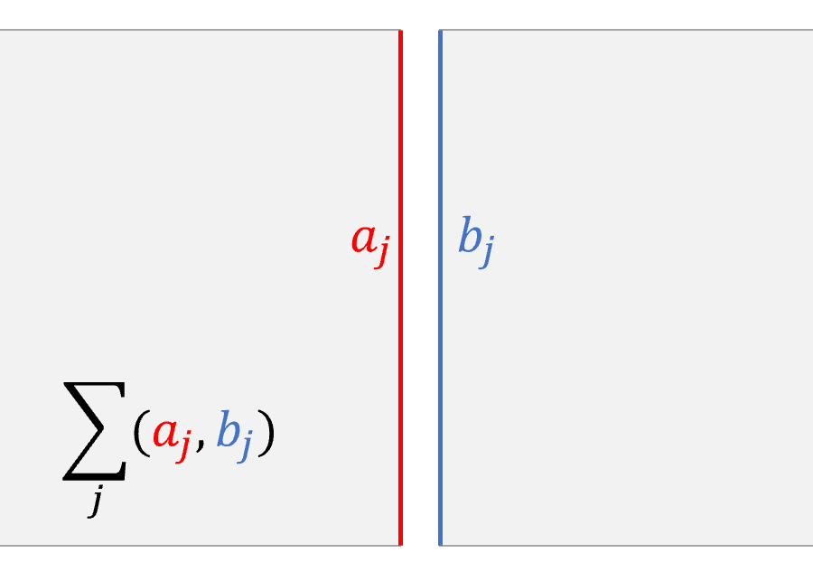
Figure B.4: A factorizing defect is (a nonnegative integer sum of) a pair of boundary conditions, one on on either side of the defect

Indeed, one way to make such a defect is to consider a small strip of gapped phase between $\mathcal{T}_{L}$ and $\mathcal{T}_{R}$ and then take this gap to infinity. If this gapped phase is degenerate, then we get a sum of factorizing defects, which can give some superselection rules for the correlation functions, which are now written as a sum of products of left and right correlation functions.

If we have a chain on a loop with two factorizing defect insertions, those defect insertions effectively slice the chain into two strands, which we may call the $A$ strand and $B$ strand. Conformal symmetry can act independently on each strand. Thus, the actual emergent algebra in the low energy theory is $Vir^{A}\otimes Vir^{B}$ (note it is an entirely different symmetry than the holomorphic-antiholomprhic $Vir\otimes\overline{Vir}$ symmetry in a model with no boundaries and defects). Likewise, a loop with only one factorizing defect insertion only has a symmetry algebra of $\cong Vir$, and more generally a loop with $n$ factorizing defect insertions separated by long distances has symmetry algebra $\cong Vir^{\otimes n}$

B.3.2 Topological defects

A topological defect is any conformal defect that is symmetric under the full $Vir\otimes\overline{Vir}$ symmetry algebra of the defect-free theory. This includes the symmetries that change its position. Correlation functions in the presence of a topological defect are unchanged if the topological defect is continuously deformed conformally without passing through any operator insertions or any other defects. Topological defects can be thought of as the opposite extreme compared to factorizing defects, in that they are essentially transparent between both sides. When a topological defect $\mathcal{L}$ wraps around a local operator insertion $\phi(z,\bar{z})$, the defect and the local operator can together be replaced by a different local operator $\mathcal{L}\phi(z,\bar{z})$ (possibly just $\phi$ multiplied by a coefficient), see Fig. B.5. This defines an action of a topological defect on the set of local operators. This also presumes an orientation of the topological defect line.

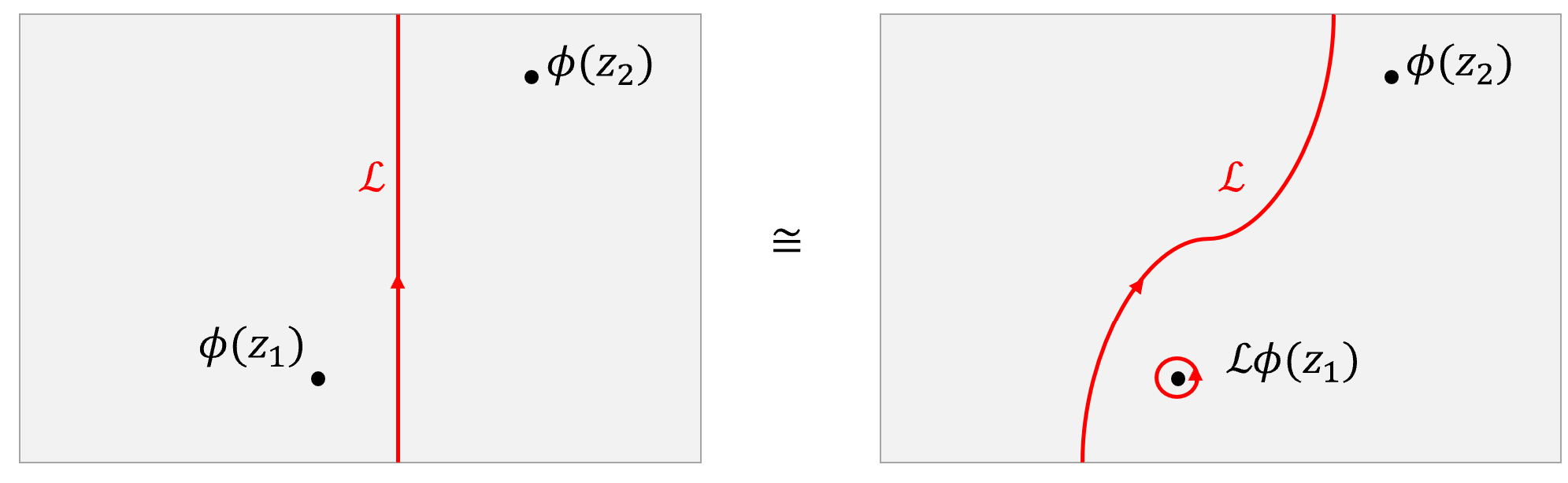
Figure B.5: A topological defect commutes with the conformal symmetry and thus can be deformed continuously without affecting any correlation functions. When passing through operator insertions it acts on those operators by wrapping around them.

When a topological defect is near another defect, the two defects can fuse along the region they are closely parallel, i.e. they can be replaced in that region by a different defect (possibly a sum of defects) that is considered the fusion product. The fusion of two topological defects is also topological. The fusion of a topological defect and a factorizing defect is also factorizing. Phase-related subtleties in the fusion of topological defects are captured by what are known as $F$ symbols.

A topological defect can be written as a sum of one or more simple topological defects. One important example of simple topological defects are symmetry defect lines. All one-site symmetry group elements $g\in G$ of the theory correspond to topological defects $\mathcal{L}_{g}$. Symmetry defect lines fuse with each other by the fusion rule $\mathcal{L}_{g}\times\mathcal{L}_{h}=\mathcal{L}_{gh}$ (in the case of non-abelian groups, the fusion product notation presumes a particular ordering convention, e.g. the first defect is to the left of the second defect). The symmetry defect line acts on local operators the same way the group $G$ act on it. A single symmetry defect line parallel to the axis of a space-time cylinder corresponds to twisted periodic boundary conditions. A lattice realization of a symmetry defect can be explicitly established by applying the symmetry action to a semi-infinite region (say sites $j>0$) of an infinite chain; this will locally alter the Hamiltonian at sites $j\approx 0$ while leaving the rest of it unchanged.

Another important example is the orbifold defect $\mathcal{N}_{G}$ which exists between a theory $\mathcal{T}$ and its orbifold $\mathcal{T}/G$ (which may be $\cong\mathcal{T}$ in self-dual theories, as is the case for the Potts KW defect $\mathcal{N}$ in the next section). This defect implements gauging by a symmetry subgroup $G$, see section B.7 for details.

B.4 DCFT of the Potts model

The complete set of defects of the Potts model is unknown. However, the set of factorizing and topological defects are completely known.

B.4.1 Factorizing defects of the Potts model

As mentioned previously, there are 8 simple boundary conditions of the Potts model, and correspondingly there are 64 simple factorizing defects. On the lattice, a factorizing defect can be realized by completely decoupling a bond of the Potts chain. Compound factorizing defects can also be realized through lattice terms that spontaneously select certain pairs of boundary conditions on either side of the decoupled bond. Furthermore, adding irrelevant perturbations, including perturbations that do couple either side of the broken bond, do not change the underlying conformal defect.

B.4.2 Topological defects of the Potts model

There are exactly 16 simple topological defects of the Potts model. Six of them are the symmetry defect lines from the $S_{3}$ symmetry group. They are the identity defect $1$, the $\mathbb{Z}_{3}$ twist defect $\eta$, a charge conjugation defect $\mathcal{C}$ and all group-like products of these. In addition to these invertible symmetry defects, there are two distinct Kramers-Wannier duality defects, $\mathcal{N}$ and $\mathcal{N^{\prime}}=\mathcal{C}\mathcal{N}$. They both satisfy $\mathcal{N}^{2}=\mathcal{N^{\prime}}^{2}=1+\eta+\eta^{2}$ and $\mathcal{N}\eta=\eta\mathcal{N}=\mathcal{N}$, are non-invertible, and implement the $\mathbb{Z}_{3}$ orbifolding procedure. For simplicity in this section we focus only on these 8 topological defects with clear physical interpretations. Furthermore there is a Fibonacci-like defect $\tau$ satisfying the fusion rule ${\tau}^{2}=\tau+1$, and one can define 8 simple defects by the fusion of $\tau$ with the symmetry and duality defects mentioned prior. Petkova and Zuber (2001); Vanhove et al. (2022); Chang et al. (2019)

Lattice realizations: We can explicitly realize some of these defects in the form of an insertion parallel to the time direction, by applying a transformation to half a quantum chain.

Defect	A possible lattice form of Hamiltonian with that insertion
1	$\ldots-X_{0}-Z_{0}Z_{1}^{\dagger}-X_{1}-Z_{1}Z_{2}^{\dagger}-X_{2}-Z_{2}Z_{3}^{\dagger}\ldots+h.c.$
$\eta$	$\ldots-X_{0}-Z_{0}Z_{1}^{\dagger}-X_{1}\color[rgb]{1,0,0}-\omega Z_{1}Z_{2}^{\dagger}\color[rgb]{0,0,0}-X_{2}-Z_{2}Z_{3}^{\dagger}\ldots+h.c.$
$\eta^{2}$	$\ldots-X_{0}-Z_{0}Z_{1}^{\dagger}-X_{1}\color[rgb]{1,0,0}-\omega^{2}Z_{1}Z_{2}^{\dagger}\color[rgb]{0,0,0}-X_{2}-Z_{2}Z_{3}^{\dagger}\ldots+h.c.$
$\mathcal{C}$	$\ldots-X_{0}-Z_{0}Z_{1}^{\dagger}-X_{1}\color[rgb]{1,0,0}-Z_{1}Z_{2}\color[rgb]{0,0,0}-X_{2}-Z_{2}Z_{3}^{\dagger}\ldots+h.c.$
$\mathcal{N}$	$\ldots-X_{0}-Z_{0}Z_{1}^{\dagger}-X_{1}\color[rgb]{1,0,0}-Z_{1}X_{2}^{\dagger}\color[rgb]{0,0,0}-Z_{2}Z_{3}^{\dagger}-X_{3}\ldots+h.c.$
	or
	$\ldots-Z_{-1}Z_{0}^{\dagger}-X_{0}-Z_{0}Z_{1}^{\dagger}\color[rgb]{1,0,0}-X_{1}Z_{2}\color[rgb]{0,0,0}-X_{2}-Z_{2}Z_{3}^{\dagger}\ldots+h.c.$

In these examples the defect is inserted at the bond between sites $1$ and $2$, but in reality that is just an arbitrary choice; physics will be the same if one writes the Hamiltonian with the same defect between sites $j$ and $j+1$ instead. One can see this explicitly by just applying the transformation unitarily on the interval between $2$ and $j$. These are not the only lattice realizations of defects; for example adding an irrelevant defect perturbation also results in the same defect. Sometimes, requiring a global symmetry of a Hamiltonian to remain unbroken (for example the global $\mathbb{Z}_{3}$) forbids certain topological defects (for example $\mathcal{N}$) from existing in an isolated manner corresponding to a local perturbation.

Actions on operators and boundaries: The topological defects have the following actions on the bulk local Virasoro primaries of the Potts model Chang et al. (2019), where here $\varphi=\frac{1+\sqrt{5}}{2}$ and $\tilde{\varphi}=\frac{1-\sqrt{5}}{2}$:

	$1$	$\epsilon$	$\phi$	$\phi^{\dagger}$	$\sigma$	$\sigma^{\dagger}$	$X$	$Y$	$\Phi_{X\bar{\epsilon}}$	$\Phi_{\epsilon\bar{X}}$	$W$	$\bar{W}$
$\eta$	$1$	$\epsilon$	$\omega\phi$	$\bar{\omega}\phi^{\dagger}$	$\omega\sigma$	$\bar{\omega}\sigma^{\dagger}$	$X$	$Y$	$\Phi_{X\bar{\epsilon}}$	$\Phi_{\epsilon\bar{X}}$	$W$	$\bar{W}$
$\mathcal{C}$	$1$	$\epsilon$	$\phi^{\dagger}$	$\phi$	$\sigma^{\dagger}$	$\sigma$	$X$	$Y$	$-\Phi_{X\bar{\epsilon}}$	$-\Phi_{\epsilon\bar{X}}$	$-W$	$-\bar{W}$
$\mathcal{N}$	$\sqrt{3}$	$-\sqrt{3}\epsilon$	$0$	$0$	$0$	$0$	$\sqrt{3}X$	$-\sqrt{3}Y$	$\sqrt{3}\Phi_{X\bar{\epsilon}}$	$-\sqrt{3}\Phi_{\epsilon\bar{X}}$	$-\sqrt{3}W$	$\sqrt{3}\bar{W}$
$\tau$	$\varphi$	$\tilde{\varphi}\epsilon$	$\varphi\phi$	$\varphi\phi^{\dagger}$	$\tilde{\varphi}\sigma$	$\tilde{\varphi}\sigma^{\dagger}$	$\tilde{\varphi}X$	$\varphi Y$	$\tilde{\varphi}\Phi_{X\bar{\epsilon}}$	$\tilde{\varphi}\Phi_{\epsilon\bar{X}}$	$\varphi W$	$\varphi\bar{W}$

Here when we write that a defect acts on 1 to result a larger number like $\sqrt{3}$ or $\varphi$, we are referring to a value that is consistent with the non-invertible nature of such defects. These values in the first column form a scalar representation of the topological defect fusion algebra. In fact they are none other than the $g_{D}$ values for each topological defect $D$.

On an open chain (or equivalently on a chain with a factorizing defect), the effect of topological defects can be understood by moving them to the boundary and fusing them to get an equivalent system with possibly-different boundary conditions. Topological defects fuse with Potts boundary conditions as in Table 6.

	fixed-$\omega^{a}$	free	mixed-$\omega^{a}$	new
$\eta$	fixed-$\omega^{a+1}$	free	mixed-$\omega^{a+1}$	new
$\mathcal{C}$	fixed-$\omega^{-a}$	free	mixed-$\omega^{-a}$	new
$\mathcal{N}$	free	$\sum_{j=0}^{2}(\textrm{fixed}-\omega^{j})$	new	$\sum_{j=0}^{2}(\textrm{mixed}-\omega^{j})$

Table 6: The action of topological defects on the Potts boundary conditions

Parition functions of twisted sectors: On a closed chain with a single topological defect insertion $D$ parallel to the timelike direction, the Hilbert space $\mathcal{H}_{D}$ (also called the $D-$twisted sector) is described by the partition function $\mathcal{Z}_{D}$, which is a sesquilinear sum of characters as functions of $q=\exp(-2\pi\beta/L)$ Vanhove et al. (2022); Petkova and Zuber (2001).

$$\begin{split}\mathcal{Z}_{1}\equiv\mathcal{Z}_{Potts}&=|\chi_{I}|^{2}+|\chi_{\epsilon}|^{2}+2|\chi_{2/3}|^{2}+2|\chi_{1/15}|^{2}\\ \mathcal{Z}_{\eta}=\mathcal{Z}_{\bar{\eta}}&=\chi_{I}\bar{\chi}_{2/3}+c.c.+\chi_{\epsilon}\bar{\chi}_{1/15}+c.c.+|\chi_{2/3}|^{2}+|\chi_{1/15}|^{2}\\ \mathcal{Z}_{C}=\mathcal{Z}_{C\eta}=\mathcal{Z}_{C\eta^{2}}&=|\chi_{u}|^{2}+|\chi_{v}|^{2}\\ \mathcal{Z}_{N}=\mathcal{Z}_{CN}^{*}&=(\chi_{I}+2\chi_{2/3})\bar{\chi}_{u}+(\chi_{\epsilon}+2\chi_{1/15})\bar{\chi}_{v}\\ \mathcal{Z}_{\tau}&=\chi_{I}\bar{\chi}_{\epsilon}+c.c.+2\chi_{2/3}\bar{\chi}_{1/15}+c.c.+|\chi_{\epsilon}|^{2}+2|\chi_{1/15}|^{2}\\ \mathcal{Z}_{\tau\eta}=\mathcal{Z}_{\tau\bar{\eta}}&=\chi_{1/15}(\bar{\chi}_{I}+\bar{\chi}_{\epsilon}+\bar{\chi}_{2/3})+c.c.+\chi_{2/3}\bar{\chi}_{\epsilon}+c.c+|\chi_{1/15}|^{2}\\ \mathcal{Z}_{\tau C}=\mathcal{Z}_{\tau C\eta}=\mathcal{Z}_{\tau C\eta^{2}}&=\chi_{u}\bar{\chi}_{v}+c.c.+|\chi_{v}|^{2}\\ \mathcal{Z}_{\tau N}=\mathcal{Z}_{\tau CN}^{*}&=\chi_{v}(\bar{\chi}_{I}+\bar{\chi}_{\epsilon}+2\bar{\chi}_{2/3}+2\bar{\chi}_{1/15})+\chi_{u}(\bar{\chi}_{\epsilon}+2\bar{\chi}_{1/15})\\ \end{split}$$ (15)

Here $\chi_{I}=\chi_{0}+\chi_{3}$, $\chi_{\epsilon}=\chi_{2/5}+\chi_{7/5}$ are $\mathcal{W}$ characters, we have also introduced for convenience $\chi_{u}=\chi_{1/8}+\chi_{13/8}$ and $\chi_{v}=\chi_{1/40}+\chi_{21/40}$, and $c.c.$ refers to the complex conjugate of the preceding term.

These partition functions show us the dimensions of operators living at the defect’s endpoint. For example, the dimension $(1/15,1/15)$ operator indicated in $\mathcal{Z}_{\eta}$ is the disorder operator $\mu$ from the $\mathbb{Z}_{3}$ twisted sector.

B.4.3 Defect RG flows

Usually, adding a relevant perturbation (a defect operator of dimension $<1$) to the site of a defect triggers an RG flow to another defect, generally with lower $g$ value, while leaving the bulk CFT unchanged.

For a topological defect all local bulk operators can be added to the site of a topological defect (but this is not the case for a general conformal defect). In the Potts model, topological defects are unstable because the thermal operator $\epsilon(z,\bar{z})$ has dimension $4/5<1$ and is usually symmetry-allowed. In Appendix  D we will argue that depending on sign, this perturbaton will drive a topological defect to itself fused with either $(f,f)$ or with $(A,A)+(B,B)+(C,C)$. The Potts topological defects’ $g$ values are $g_{I}=g_{\eta}=g_{\mathcal{C}}=1$, $g_{\mathcal{N}}=\sqrt{3}$, $g_{\tau}=\frac{1+\sqrt{5}}{2}$.

B.5 Modular tensor category interpretation of topological defects and boundary conditions

For minimal models, a modular tensor category description can be used to read off the boundary partition functions $\mathcal{Z}_{ab}$ and the actions of topological defects Vanhove et al. (2022). Chiral Virasoro primaries, topological defects, and boundary conditions are objects categories $\mathcal{D}$, $\mathcal{C}$, and $\mathcal{M}$ respectively, where $\mathcal{M}$ is a left-right $(\mathcal{C},\mathcal{D})$ -bimodule category. The module action of $\mathcal{C}$ on $\mathcal{M}$ indicates the fusion of topological defects with boundary conditions. If the module action of $\mathcal{D}$ on $\mathcal{M}$ is $h:a\to\sum_{b\in\mathcal{M}}n^{h}_{ab}b$, then $\mathcal{Z}_{ab}=\sum_{h\in\mathcal{D}}n^{h}_{ab}\chi_{h}$. The fusion rules within $\mathcal{C}$ and $\mathcal{D}$ match those of fields and defects respectively.

We demonstrate this for the Potts model. $\mathcal{C}_{\textrm{Potts}}=\mathcal{C}_{S_{3}}\otimes Fib$, where $Fib$ is the Fibonacci category containing two simple objects $1,\tau$ with fusion rule $\tau^{2}=\tau+1$, and $\mathcal{C}_{S_{3}}$ is a fusion category containing six objects forming the $S_{3}$ group as well as two duality objects $\mathcal{N}$ and $\mathcal{N}^{\prime}$. $\mathcal{D}_{\rm Potts}=|su(2)_{4}|\otimes Fib$, where $|su(2)_{4}|$ has five simple objects $0,1/2,1,3/2$, and $2$. The correspondence between $\mathcal{D}_{\rm Potts}$ and $c=8/5$ primary dimensions is

	0	1/2	1	3/2	2
1	0	1/8	2/3	13/8	3
$\tau$	2/5	1/40	1/15	21/40	7/5

$\mathcal{M}_{\textrm{Potts}}=\mathcal{M}_{TY}\otimes Fib$, where $\mathcal{M}_{TY}$ is the $\mathbb{Z}_{3}$ Tambara-Yamagami category (containing objects $A,B,C\in\mathbb{Z}_{3}$ and $f$ satisfying $f\times f=A+B+C$). The mixed and new boundary conditions correspond to $\tau\in Fib$ while fixed and free correspond to $1\in Fib$. $Fib$ acts as a module over itself, while $|su(2)_{4}|$ and $C_{S_{3}}$ actions on $M_{TY}$ are consistent with the partition functions and topological defect actions mentioned earlier.

B.6 Boundary State Formalism

Earlier in this appendix we focused on the quantization scheme around a boundary point, the “open string” picture. However, we can also consider time slices parallel to the boundary, the “closed string” picture. This is conveniently expressed on a disk (or annulus) with radial quantization. Then the Hilbert space and conformal algebra are the same as in the boundary-less case (i.e. the conformal algebra is $Vir\otimes\overline{Vir}$ and the Hilbert space $\mathcal{H}_{\rm bulk}$ is a direct sum of some irreducible representations of $Vir\otimes\overline{Vir}$). The boundary condition $a$ at the boundary corresponds to a boundary state $|a\rangle\in\mathcal{H}_{\rm bulk}$. The boundary state satisfies many constraints including the boundary conformal invariance condition $(L_{m}-\bar{L}_{-m})|a\rangle=0$ for all $m\in\mathbb{Z}$. Here $L_{m}$ and $\bar{L}_{m}$ are $Vir\otimes\overline{Vir}$ generators for the closed string quantization scheme (see the disk in Fig. B.6(a)) and are different from the $Vir$ generators of section B.1. These boundary states need not be normalizable, and contrary to usual quantum intuition, $|a\rangle$ and $k|a\rangle$ are not physically the same for arbitrary scalars $k$ (for most generic non-integer $k$, $k|a\rangle$ is not even a boundary state at all). Boundary states do not form a vector space over $\mathbb{C}$; however semigroup-like addition of boundary states is encoded by adding nonnegative integer linear combinations.

Figure B.6: The boundary state formalism. (a) The closed string quantization scheme is conveniently described on a finite disk geometry. With radial quantization, the boundary is characterized by a boundary state $|a\rangle$ that obeys the conformal invariance condition $L_{m}|a\rangle=\bar{L}_{-m}|a\rangle$ (as well as various other stringent mathematical constraints). (b) An annulus with two boundaries can be mapped to the same cylindrical geometry used to compute the finite temperature partition function of a quantum chain. However with radial quantization, this has the interpretation of a propagator for time evolution from $|b\rangle$ to $|a\rangle$

Using an exponential mapping, an annulus-shaped space-time surface can be expressed as a cylinder of finite length with two boundaries, with boundary condition $a$ on one boundary circle and $b$ on the boundary circle. $\mathcal{Z}_{ab}$ had the interpretation of a finite-temperature partition function of an open chain in the open string picture. But the closed string picture, $\mathcal{Z}_{ab}$ is actually a time evolution amplitude from boundary state $|a\rangle$ to boundary state $|b\rangle$ for time $L$ and spatial circumference $\beta$. (Here $\tilde{q}\equiv\exp(-4\pi L/\beta)$.)

$$\mathcal{Z}_{ab}=\langle b|\sqrt{\tilde{q}}^{L_{0}+\bar{L}_{0}-c/12}|a\rangle$$

Generally, finding the boundary states is a hard problem; among other things it requires solving consistency conditions for $\mathcal{Z}_{ab}$ between open-string and closed-string. However, for diagonal minimal models there is an elegant solution by Cardy Cardy (1989); Runkel (2000); Di Francesco et al. (1997). In a diagonal model for any spinless primary $\phi_{h,h}(z,\bar{z})$ we can define an “Ishibashi state” $|\phi\rangle\rangle$ that is annihilated by $L_{m}-\bar{L}_{-m}$.

$$|\phi\rangle\rangle=\sum_{J}|\phi,J\rangle\otimes U|\overline{\phi,J}\rangle$$

Here, the tensor product is between a $Vir$ irrep and a $\overline{Vir}$ irrep, $|\phi,J\rangle$ is the $J$-th $Vir$ descendant of the chiral primary $\phi$, and $U$ is an antiunitary operator commuting with $\overline{Vir}$.

The Ishibashi state is not a boundary state but can be used as a basis to construct the boundary states. To do so, there is a remarkable and nontrivial one-to-one correspondnece between simple boundary states and spinless primary operators $j$. To disambiguate notation, here we will specify $|j\rangle_{bdy}$ to be the boundary state that is in correspondence with spinless primary $j$. Then if $S$ is the modular $S$ matrix such that $\chi_{\ell}(\tilde{q})=S_{k\ell}\chi_{k}(q)$ we can explicitly write down

$$|j\rangle_{bdy}=\sum_{k}\frac{S_{kj}}{\sqrt{S_{0j}}}|k\rangle\rangle$$ (16)

The Potts model is not a Virasoro diagonal model. However, a similar approach can be used to exactly write down its boundary states Mong et al. (2014). They are:

$$|\textrm{fixed}-\omega^{a}\rangle =N\left(|I\rangle\rangle+\omega^{a}|\psi\rangle\rangle+\omega^{-a}|\psi^{\dagger}\rangle\rangle+\sqrt{\varphi}\left(|\epsilon\rangle\rangle+\omega^{a}|\sigma\rangle\rangle+\omega^{-a}|\sigma^{\dagger}\rangle\rangle\right)\right)$$ (17)

$$|\textrm{free}\rangle =N\sqrt{3}\left(|0\rangle\rangle-|3\rangle\rangle-\sqrt{\varphi}|2/5\rangle\rangle+\sqrt{\varphi}|7/5\rangle\rangle\right)$$ (18)

$$|\textrm{mixed}-\omega^{a}\rangle =N\left(\varphi\left(|I\rangle\rangle+\omega^{a}|\psi\rangle\rangle+\omega^{-a}|\psi^{\dagger}\rangle\rangle\right)+\sqrt{1/\varphi}\left(|\epsilon\rangle\rangle+\omega^{a}|\sigma\rangle\rangle+\omega^{-a}|\sigma^{\dagger}\rangle\rangle\right)\right)$$ (19)

$$|\textrm{new}\rangle =N\sqrt{3}\left(\varphi|0\rangle\rangle-\varphi|3\rangle\rangle+\sqrt{1/\varphi}|2/5\rangle\rangle-\sqrt{1/\varphi}|7/5\rangle\rangle\right)$$ (20)

Here $\varphi=\frac{1+\sqrt{5}}{2}$, the golden ratio, and $N=\left(\frac{5-\sqrt{5}}{30}\right)^{1/4}$. We have denoted Ishibashi states $|I\rangle\rangle=|0\rangle\rangle+|3\rangle\rangle$ and $|\epsilon\rangle\rangle=|2/5\rangle\rangle+|7/5\rangle\rangle$, while $|\psi\rangle\rangle$ and $|\psi^{\dagger}\rangle\rangle$ are the charged Ishibashi states corresponding to chiral primaries $\psi$ and $\psi^{\dagger}$ and similarly for $\sigma$. Note that the coefficient of the lowest-dimensional Ishibashi state is the same as the Affleck-Ludwig $g$ value from (14).

A conformal defect parallel to a time slice is an operator acting on $\mathcal{H}_{\rm bulk}$. For example, a factorizing defect composed of two boundary conditions $(a,b)$ can be heuristically thought of as the operator $|b\rangle\langle a|$. Then fusion of defects is given by operator multiplication, and fusion of defects with boundaries is given by operators acting on boundary states.

B.7 BCFT of an Orbifold

If we have a CFT $\mathcal{T}$ with a finite, anomaly-free symmetry $G$, we can form the $G$-orbifold $\mathcal{T}/G$ by gauging the symmetry. The local operators of $\mathcal{T}/G$ are of two kinds, one being those local operators of $\mathcal{T}$ which are $G$-invariant. The others are twist operators, which come from the $G$-invariant $G$-string operators of $\mathcal{T}$. This is the same sense of string operator we used to describe SPT phases—these are the operators living at the ends of a half-infinite $g$ operator for some $g\in G$. $\mathcal{T}/G$ has a global symmetry, called the magnetic symmetry, for which the charge of a local operator of $\mathcal{T}/G$ is its twist $g\in G$. For abelian $G$, this is a $G^{\vee}={\rm Hom}(G,U(1))\cong G$ global symmetry, but the generators form the ring of characters ${\rm Rep}(G)$ in general.

These local operators correspond with the states of the theory, and there is a similar mapping of the boundary conditions, which may also be identified with Cardy states. In particular, if $|B\rangle$ is a Cardy state of $\mathcal{T}$,

$$|B^{G}\rangle=\frac{1}{\sqrt{|G|}}\sum_{g}g|B\rangle$$ (21)

is a Cardy state of $\mathcal{T}/G$, where $g|B\rangle$ denotes the $G$ action in the Hilbert space. However, if $|B\rangle$ is $K$-invariant for some $K<G$, meaning for all $g\in K$, $g|B\rangle=|B\rangle$, then $|B^{G}\rangle$ will be reducible, since $\langle B^{G}|B^{G}\rangle$ contains $|K|\langle B|B\rangle$, and therefore this boundary has $|K|$ different vacuum operators. In fact if $K$ is the maximal such subgroup then $|B^{G}\rangle$ has precisely $|K|$ different vacuum operators. By diagonalizing these, it splits into a sum of $|K|$ different Cardy states of $\mathcal{T}/G$. If $|B\rangle$ was not reducible in $\mathcal{T}$, then this splitting must involve the twisted sector operators of $\mathcal{T}/G$ and therefore these states break the magnetic symmetry. In fact we can argue that $|B^{G}\rangle$ spontaneously breaks ${\rm Rep}(G)$ down to ${\rm Rep}(G/K)$, where ${\rm Rep}(G/K)$ are the $G$-representations containing a $K$-fixed vector, or simply $(G/K)^{\vee}$ in the abelian case.

More abstractly, there exists a topological defect which we call the orbifold defect $\mathcal{N}_{G}$ between $\mathcal{T}$ and $\mathcal{T}/G$, obtained using Dirichlet boundary conditions for the $G$ gauge field, or equivalently only summing over closed $G$ line defects on one side of $\mathcal{N}_{G}$ (See Section 2.4 and Fig. 6 of Thorngren and Wang (2021) and also Bhardwaj and Tachikawa (2018)). There is also a dual defect $\mathcal{N}_{G}^{\vee}$ going the other way, which equivalently may be described by partial ${\rm Rep}(G)$ gauging. This defect satisfies the fusion rule

$$\begin{split}\mathcal{N}_{G}^{\vee}\otimes\mathcal{N}_{G}&=\sum_{g}g\\ \mathcal{N}_{G}\otimes\mathcal{N}_{G}^{\vee}&=\sum_{\chi\in G^{\vee}}\chi.\end{split}$$ (22)

We can fuse boundary conditions of $\mathcal{T}$ with $\mathcal{N}_{G}$ to get boundary conditions of $\mathcal{T}/G$, ie. $\mathcal{N}_{G}|B\rangle=|B^{G}\rangle$, and vice versa for $\mathcal{N}_{G}^{\vee}$ and gauging the magnetic symmetry. Note $\mathcal{N}_{G}^{\vee}|B^{G}\rangle=|G||B\rangle$.

B.7.1 Ising Orbifold BCFT and Kramers-Wannier Duality

For example, let us consider three simple Cardy states of the Ising CFT, corresponding to the free and two fixed boundary conditions

$$\begin{gathered}|{\rm free}\rangle=|1\rangle\rangle-|\epsilon\rangle\rangle\\ |{\rm fixed}\pm\rangle=\frac{1}{\sqrt{2}}|1\rangle\rangle+\frac{1}{\sqrt{2}}|\epsilon\rangle\rangle\pm\frac{1}{2^{1/4}}|\sigma\rangle\rangle\end{gathered}$$

where we have used $|\phi\rangle\rangle$ to label the Ishibashi state corresponding to the primary $\phi$. Under the $\mathbb{Z}_{2}$ spin-flip symmetry $P$, the fixed boundary conditions are not symmetric, since

$$P|\sigma\rangle\rangle=-|\sigma\rangle\rangle.$$

Thus, we can make only two $\mathbb{Z}_{2}$-symmetric Cardy states out of the above, namely $|{\rm free}\rangle$ and “spontaneously fixed”

$$|{\rm spontfixed}\rangle=|{\rm fixed}+\rangle+|{\rm fixed}-\rangle=\sqrt{2}|1\rangle\rangle+\sqrt{2}|\epsilon\rangle\rangle.$$

If we apply the gauging map above, we get

$$\begin{gathered}|{\rm free}^{\mathbb{Z}_{2}}\rangle=\sqrt{2}|1\rangle\rangle-\sqrt{2}|\epsilon\rangle\rangle\\ |{\rm fixed}\pm^{\mathbb{Z}_{2}}\rangle=|1\rangle\rangle+|\epsilon\rangle\rangle\end{gathered}$$

Note both fixed boundary conditions get mapped to the same boundary condition of the orbifold, since we sum over the $\mathbb{Z}_{2}$ orbit.

Because of Kramers-Wannier duality, we can identify the $\mathbb{Z}_{2}$-orbifold of Ising with Ising itself, via the map

$$\begin{gathered}|1\rangle\mapsto|1\rangle\\ |\epsilon\rangle\mapsto-|\epsilon\rangle\end{gathered}$$

We see

$$\begin{gathered}|{\rm free}\rangle\mapsto|{\rm spontfixed}\rangle\\ |{\rm fixed}\pm\rangle\mapsto|{\rm free}\rangle.\end{gathered}$$

Observe that the $\mathbb{Z}_{2}$-symmetric free boundary maps to the $\mathbb{Z}_{2}^{\vee}$-SSB boundary, and vice versa. As claimed the $\mathbb{Z}_{2}$-symmetric $|{\rm free}\rangle$ boundary maps to one that splits when we include the twisted sectors, which in the dual variables are the $|\sigma\rangle\rangle$ terms in $|{\rm fixed}\pm\rangle$.

Appendix C Mapping to single Potts chain

The cluster model has an elegant nonlocal unitary mapping to two decoupled Potts chains. We use this mapping extensively to take advantage of the well known properties of the Potts model and the Potts CFT in our analysis of our cluster SPT transition. In the presence of a boundary (with boundary perturbations), the mapping sends the open-chain cluster model to two open Potts chains coupled only at their endpoints, which can in turn be “unfolded” and viewed as a single closed-loop Potts chain of twice the length with some defects.

C.1 Mapping of infinite chain

We will write down an exact unitary mapping from the cluster model $H_{\omega}+H_{\bar{\omega}}$ to a model of two decoupled critical three-state Potts chains. Our mapping is such that gauging the odd symmetry $\mathbb{Z}^{o}_{3}$ of the cluster model results in the Potts² model. Conversely gauging the antidiagonal symmetry $\mathbb{Z}^{(1,-1)}_{3}$ of Potts² results in the cluster model. The mapping is depicted schematically in Fig. 3.

As an outline, to do so, we first apply a Kramers-Wannier transformation on just the odd sites of the cluster model, mapping those variables to link variables $\hat{X}_{2j}$ and $\hat{Z}_{2j}$ that live on some auxiliary even sites. Then for each position $2j$ we canonically reparametrize the cluster chain variables $X_{2j},Z_{2j}$ on the original physical site $2j$ and the link variables $\hat{X}_{2j},\hat{Z}_{2j}$ into variables $\tilde{X}^{A}_{2j},\tilde{X}^{B}_{2j},\tilde{Z}^{A}_{2j},\tilde{Z}^{B}_{2j}$. These variables then end up conveniently describing the cluster model in the form of two decoupled Potts chains.

Kramers-Wannier step: We define auxiliary link variables as follows:

$$\hat{X}_{2j}\equiv Z_{2j-1}Z_{2j+1}^{\dagger} \hat{Z}_{2j}\equiv\prod_{k<j}X^{\dagger}_{2k-1}$$

Reparametrization as $A$ and $B$ chains: We define the Potts² variables $\tilde{X}^{A}_{2j},\tilde{X}^{B}_{2j},\tilde{Z}^{A}_{2j},\tilde{Z}^{B}_{2j}$ as follows:

$$X_{2j}\equiv\tilde{X}^{A}_{2j}\tilde{X}^{B}_{2j}\qquad Z_{2j}\equiv\tilde{Z}^{A\dagger}_{2j}\tilde{Z}^{B\dagger}_{2j}\qquad\hat{X}_{2j}\equiv\tilde{X}^{A\dagger}_{2j}\tilde{X}^{B}_{2j}\qquad\hat{Z}_{2j}\equiv\tilde{Z}^{A}_{2j}\tilde{Z}^{B\dagger}_{2j}$$

This manifestly decouples the two Potts chains to which the cluster model maps.

Overall mapping: The exact map from Potts² variables ($\bigotimes_{j\in\mathbb{Z}}\mathbb{C}^{3}_{2j,A}\otimes\mathbb{C}^{3}_{2j,B}$) to cluster ($\bigotimes_{j\in\mathbb{Z}}\mathbb{C}^{3}_{j}$) variables is shown in table 7. In particular, the Hamiltonian maps as follows:

$$\begin{split}-H&=\sum_{j}\left(X_{j}+X_{j}^{\dagger}\right)\left(Z_{j-1)}Z_{j+1}^{\dagger}+Z_{j-1}^{\dagger}Z_{j+1}\right)\\ -H&=\sum_{j}\left(\tilde{Z}^{A}_{2j}\tilde{Z}^{A\dagger}_{2(j+1)}+\tilde{X}^{A}_{2j}+h.c.\right)+(A\Leftrightarrow B)\end{split}$$ (23)

Here for technical convenience we defined each Potts chain to only have sites labeled by even integers $\ldots 2j-2,2j,2j+2\ldots$; i.e. site $2j$ and site $2j+2$ are adjacent.

Potts2	Cluster
$\tilde{X}_{2j}^{A}\tilde{X}_{2j}^{B}$	$X_{2j}$
$\tilde{Z}_{2j}^{A\dagger}\tilde{Z}_{2j}^{B\dagger}$	$Z_{2j}$
$\tilde{Z}_{2j-2}^{A}\tilde{Z}_{2j-2}^{B\dagger}\tilde{Z}_{2j}^{A\dagger}\tilde{Z}_{2j}^{B}$	$X_{2j-1}$
$\prod_{k=j}^{\infty}\tilde{X}_{2k}^{A\dagger}\tilde{X}_{2k}^{B}$	$Z_{2j-1}$
$\tilde{X}_{2j}^{B}$	$Z_{2j-1}^{\dagger}X_{2j}^{\dagger}Z_{2j+1}$
$\tilde{X}_{2j}^{A}$	$Z_{2j-1}X_{2j}^{\dagger}Z_{2j+1}^{\dagger}$
$\tilde{Z}_{2j}^{A}$	$\ldots X_{-3}X_{-1}X_{1}X_{3}\ldots X_{2j-1}Z_{2j}$
$\tilde{Z}_{2j}^{B}$	$\ldots X_{-3}^{\dagger}X_{-1}^{\dagger}X_{1}^{\dagger}X_{3}^{\dagger}\ldots X_{2j-1}^{\dagger}Z_{2j}$

Potts2	Cluster
$\prod_{j}\tilde{X}^{A}_{2j}\tilde{X}^{B}_{2j}$	$\prod_{j}X_{2j}$
$\sim 1$	$\prod_{j}X_{2j-1}$
$\prod_{j}\tilde{X}^{A}_{2j}\tilde{X}^{B\dagger}_{2j}$	$\sim 1$
$(A\Leftrightarrow B)$	Charge Conj. on odd sites
$\mathcal{N}_{A}^{\prime}\mathcal{N}_{B}$	Translation by one site
$\mathcal{C}_{A}$	$X_{j}\Leftrightarrow Z_{j-1}Z^{\dagger}_{j+1}$
$\mathcal{N}_{A}^{\prime}\mathcal{N}_{B}^{-1}$	$\mathcal{K}$

Table 7: An exact equivalence between the variables of the Potts² model and cluster model. The Potts² model is defined on two chains, labeled $A$ and $B$, on even integer sites only. The cluster model is defined on one chain with all integer sites. Due to subtleties of gauging, some global symmetries do not map perfectly unitarily.

C.1.1 Mapping of symmetry actions

Although the resulting Potts model also appears to have a $\mathbb{Z}_{3}$ symmetry on each chain, it is important to note that the the $\mathbb{Z}_{3}^{e}\otimes\mathbb{Z}_{3}^{o}$ symmetry of the cluster model is not the same as the $\mathbb{Z}_{3}^{A}\otimes\mathbb{Z}_{3}^{B}$ symmetry of the Potts² model. Instead, $\mathbb{Z}_{3}^{e}$ maps to a diagonal $\mathbb{Z}_{3}$ subgroup of $\mathbb{Z}_{3}^{A}\otimes\mathbb{Z}_{3}^{B}$ (which we can call $\mathbb{Z}_{3}^{(1,1)}$) that acts the same way on both chains. Meanwhile $\mathbb{Z}_{3}^{o}$ is gauged away (its generator maps to a label of twisted sectors). The antidiagonal subgroup of $\mathbb{Z}_{3}^{A}\otimes\mathbb{Z}_{3}^{B}$ (which we can call $\mathbb{Z}_{3}^{(1,-1)}$ ) is the magnetic symmetry emerging from gauging. It is not a physical symmetry of the original model; in fact our boundary perturbations always break this symmetry.

In Table 7 we also mention how some other “accidental” symmetries of the unperturbed cluster model map, keeping in mind that we are not necessarily constraining our model and its perturbations to obey those symmetries. Charge conjugation on just odd sites maps to the operation of interchanging the $A$ and $B$ chains. Translation by one site in the cluster model maps (up to a $U^{e}$ factor) to a certain type of Kramers Wannier transformation $\mathcal{N}_{B}$ on the $B$ chain and a different type of Kramers Wannier transformation $\mathcal{N}^{\prime}_{A}=\mathcal{N}_{A}\mathcal{C}_{A}$ (a spatially flipped version of $\mathcal{N}_{A}$) on the $A$ chain. Finally, we note there is an intricate five-site unitary symmetry $\mathcal{K}$ of the cluster chain exchanging $\mathbb{Z}_{3}^{e}\Leftrightarrow\mathbb{Z}_{3}^{o}$ defined by

$$\begin{split}\mathcal{K}:X^{\dagger}_{j}&\to Z_{j-2}X_{j-1}Z_{j}X_{j+1}Z_{j+2}\\ \mathcal{K}:Z^{\dagger}_{j}&\to Z_{j-1}X_{j}Z_{j+1}\end{split}$$ (24)

This maps to KW transformation $\mathcal{N}_{A}^{\prime}$ on chain A and the inverse KW transformation $\mathcal{N}_{B}^{-1}$ on chain $B$ . We will see later that on finite open chains, the boundary generically breaks $\mathcal{K}$. However specifically at the DQCP boundary $b=1$, $\mathcal{K}$ becomes an enhanced symmetry.

C.2 Mapping of finite chains: boundaries via interface with trivial phase

To study edge modes, we must study an open chain with boundaries. Different ways of terminating endpoints give rise to different conformal boundary conditions.

In order to define the most natural cluster $\to$ Potts² mapping of boundary variables, we formalize the notion of truncation using an interface procedure (Fig. C.7). Namely, we add the trivially gapped Hamiltonian ($-\Lambda\sum_{k\not\in S}X_{k}+h.c.$) with infinite coefficient ($\Lambda\to\infty$) everywhere to the cluster model outside a finite interval $S$. Effectively this projects out all but a finite number of degrees of freedom. One is left with a finite-length cluster chain and a well defined map of its boundaries to Potts² boundaries.

$$H_{\textrm{finite},S}=-\sum_{k+1,k-1\in S}(X_{k}+h.c.)(Z_{k-1}Z_{k+1}^{\dagger}+h.c.)$$

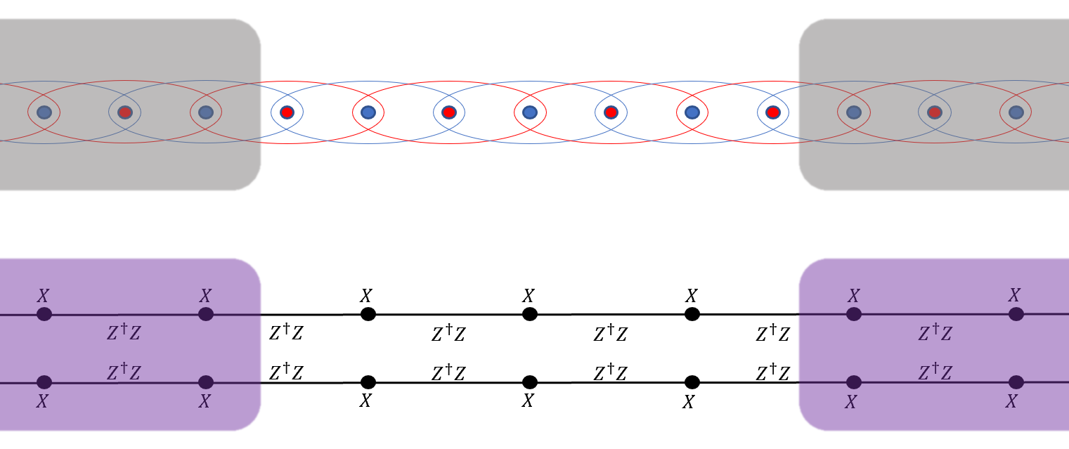
Figure C.7: Finite gapless chains can be systematically constructed by creating an interface between the gapless cluster chain and the trivially gapped phase (grey). In the Potts² language, this looks like an interface with the antidiagonal SSB (purple). The low energy physics depends significantly on the even/odd parity of the interface site.

Interestingly, the CFT is sensitive to whether we terminate at an even or odd site. In the main text, we study the case where left and right endpoints are at odd sites with on-site boundary perturbations $b(X+X^{\dagger})$. Nevertheless, it is useful to also consider even-site endpoints. This is because it turns out the odd-site endpoint with large/infinite boundary perturbation is essentially the same as the even-site endpoint with small/zero boundary perturbation, and vice versa. The relation will be made more quantitatively explicit in Appendix  D.1. Below we consider the case of both endpoints being odd and both endpoints being even. The case where one endpoint is even and the other is odd is considered in Appendix  E.

C.2.1 Odd Endpoints

Here we define an exact unitary map for boundary variables the cluster chain on sites $1\leq j\leq 2N+1$ to the Potts² model, using the interface formalism. First let us define the left boundary, applying projections $\tilde{X}^{A}_{2j}\tilde{X}^{B}_{2j}=\tilde{Z}^{A}_{2j-2}\tilde{Z}^{B\dagger}_{2j-2}\tilde{Z}^{A\dagger}_{2j}\tilde{Z}^{B}_{2j}=1$ for all $j\leq 0$. As a result, the mapping rules from Table  7 change in the following way: $\tilde{Z}^{A\dagger}_{2}\tilde{Z}^{B}_{2}=X_{1}$. Similarly, applying the projection for cluster sites $j\geq 2N+2$ leaves behind only one qutrit degree of freedom right of Potts² site $2N$, parameterized by clock matrices $Y\equiv Z^{A}_{2N+2}Z^{B\dagger}_{2N+2}$ and $W\equiv\prod_{j\geq N+1}X_{2j}^{A\dagger}X_{2j}^{B}$.

Ultimately the mapping from Table  7 takes the form of Table  8 in the presence of odd-site boundaries. It unitarily sends the cluster chain on $2N+1$ sites to two Potts chains. each on $N$ sites, along with an extra qutrit parameterized by $W$ and $Y$.

$$\begin{split}-H&=\color[rgb]{1,0,0}b_{L}\color[rgb]{0,0,0}X_{1}+\color[rgb]{1,0,0}b_{R}\color[rgb]{0,0,0}X_{2N+1}+h.c.+\sum_{j\geq 2}(X_{k}+h.c.)(Z_{k-1}Z_{k+1}^{\dagger}+h.c.)\\ -H&=\color[rgb]{1,0,0}b_{L}\color[rgb]{0,0,0}Z^{A\dagger}_{2}Z^{B}_{2}+\color[rgb]{1,0,0}b_{R}\color[rgb]{0,0,0}YZ^{A\dagger}_{2N}Z^{B}_{2N}+\sum_{j=1}^{N-1}Z^{A}_{2j}Z^{A\dagger}_{2j+2}+\sum_{j=1}^{N}X_{2j}^{A}+(A\Leftrightarrow B)+h.c.\end{split}$$ (25)

The extra qutrit is due to gauging away $\mathbb{Z}_{3}^{o}$, mapping the global $U^{o}$ generator to a local operator $Y$. One cannot naively write a one-to-one map from cluster boundary conditions to Potts² boundary conditions without addressing this gauging subtlety (see section C.4). Although we wrote $Y$ coupled to the rightmost site, we can arbitrarily relocate it by redefining $\tilde{Z}\to Y\tilde{Z}$ in some sub-interval. In fact, the extra qutrit is a topological defect insertion, which will be shown in sections C.2.2 and C.4. Furthermore, any $\mathbb{Z}_{3}^{o}\times\mathbb{Z}_{3}^{e}$-symmetric Hamiltonian must commute with $Y$, so we can treat $Y$ as just a classical label with possible values $1,\omega,\omega^{2}$.

Potts2	Cluster
$\tilde{X}_{2j}^{A}\tilde{X}_{2j}^{B}$	$X_{2\leq 2j\leq 2N}$
$\tilde{Z}_{2j}^{A\dagger}\tilde{Z}_{2j}^{B\dagger}$	$Z_{2\leq 2j\leq 2N}$
$\tilde{Z}_{2j-2}^{A}\tilde{Z}_{2j-2}^{B\dagger}\tilde{Z}_{2j}^{A\dagger}\tilde{Z}_{2j}^{B}$	$X_{3\leq 2j-1\leq 2N-1}$
$W\prod_{k=j}^{N}\tilde{X}_{2k}^{A\dagger}\tilde{X}_{2k}^{B}$	$Z_{1\leq 2j-1\leq 2N+1}$
$\tilde{Z}_{2}^{A\dagger}\tilde{Z}_{2}^{B}$	$X_{1}$
$Y^{\dagger}\tilde{Z}^{A}_{2N}\tilde{Z}^{B\dagger}_{2N}$	$X_{2N+1}$

Potts2	Cluster
$\tilde{X}_{2\leq 2j\leq 2N}^{B}$	$Z_{2j-1}^{\dagger}X_{2j}^{\dagger}Z_{2j+1}$
$\tilde{X}_{2\leq 2j\leq 2N}^{A}$	$Z_{2j-1}X_{2j}^{\dagger}Z_{2j+1}^{\dagger}$
$\tilde{Z}_{2\leq 2j\leq 2N}^{A}$	$X_{1}X_{3}\ldots X_{2j-1}Z_{2j}$
$\tilde{Z}_{2\leq 2j\leq 2N}^{B}$	$X_{1}^{\dagger}X_{3}^{\dagger}\ldots X_{2j-1}^{\dagger}Z_{2j}$
$Y$	$\prod_{j=0}^{N}X_{2j+1}^{\dagger}$
$W$	$Z_{2N+1}$

Potts2	Cluster
$\prod_{j=1}^{N}\tilde{X}^{A}_{2j}\tilde{X}^{B}_{2j}$	$\prod_{j=1}^{N}X_{2j}$
$Y^{\dagger}$	$\prod_{j=0}^{N}X_{2j+1}$
$\prod_{j=1}^{N}\tilde{X}^{A}_{2j}\tilde{X}^{B\dagger}_{2j}$	$Z_{1}Z^{\dagger}_{2N+1}$

Table 8: Odd endpoint mapping: An exact equivalence between the cluster model on an open chain with odd-site endpoints and the Potts² model. Here the cluster model is defined on all integer sites $1\leq j\leq 2N+1$. Each of the two Potts chains are defined only on even sites from $2$ to $2N$ inclusive; the Potts chains couple to an additional qutrit degree of freedom described by clock and shift matrices $Y$ and $W$.

C.2.2 Unfolding Potts² into a single closed Potts chain

We showed that the open cluster chain maps to two open Potts chains that are only coupled locally at their boundaries. In Fig. 3 we see that this is the same as one Potts chain on a squished closed loop, with some perturbations (defects) added to the parts that are bent. In the literature this general idea is called the “folding trick”. Oshikawa and Affleck (1997); Wong and Affleck (1994); Fendley et al. (2009) To be explicit, we can relabel Potts² sites as follows:

$$\mathcal{O}^{A}_{2j}\to\mathcal{O}_{j}\qquad\mathcal{O}^{B}_{2j}\to\mathcal{O}_{1-j}$$

The result is a Potts chain on a closed loop with two diametrically opposite defects parameterized by $b$, and also the option of one of three twisted periodic boundary conditions. We will refer to the lattice defect $b\tilde{Z}_{j}\tilde{Z}_{j+1}^{\dagger}$ on one bond as a “bond strength defect”.

Symmetries $\mathbb{Z}_{3}^{e}$ and $\mathbb{Z}_{3}^{o}$ and transformation $\mathcal{K}$ have elegant interpretations in this closed Potts loop. $\mathbb{Z}_{3}^{e}$ is the usual global $\mathbb{Z}_{3}$ symmetry of the Potts model. The eigenvalue of the generator of $\mathbb{Z}_{3}^{o}$ labels a twisted boundary condition of the Potts model. In other words there is an insertion of the twist-sum topological defect $1+\eta+\bar{\eta}$ (see Appendix B.4). The five-site $\mathcal{K}$ transformation introduced in Eqn. (24) is the Potts Kramers-Wannier transformation (up to some global symmetry factors). The Potts Kramers-Wannier transformation can be regarded as an exact unitary map on the finite closed lattice, exchanging global $\mathbb{Z}_{3}$ symmetry sectors with $\mathbb{Z}_{3}$ twisted sectors.

C.2.3 Even endpoints

Here we derive the mapping rules for a cluster chain on sites $0\leq j\leq 2N$. For the left endpoint, upon projection $X_{j<0}\to 1$ the two qutrits on Potts² site $0$ get reduced to one qutrit parameterized by $\tilde{Z}_{0}\equiv\tilde{Z}^{A}_{0}=\tilde{Z}^{B}_{0}$ and $\tilde{X}_{0}\equiv\tilde{X}^{A}_{0}\tilde{X}^{B}_{0}$. At the right endpoint, the projection $X_{j>2N}=1$ results in only two qutrits at sites $\geq 2N$, one which is analogous to that for the left endpoint and one of which is the twist label: $\tilde{Z}_{2N}\equiv\tilde{Z}^{A\dagger}_{2N}Z^{B\dagger}_{2N}$, $\tilde{X}_{2N}\equiv\tilde{X}_{2N}^{A}\tilde{X}_{2N}^{B}$,${Y}\equiv\tilde{Z}_{2N}^{A}\tilde{Z}_{2N}^{B\dagger}$, and ${W}\equiv\prod_{k\geq{N}}\tilde{X}_{2k}^{A\dagger}\tilde{X}_{2k}^{B}$ The mapping rules with both these endpoints are thus as shown in Table 9:

Potts2	Cluster
$\tilde{X}_{2j}^{A}\tilde{X}_{2j}^{B}$	$X_{2\leq 2j\leq 2N-2}$
$\tilde{Z}_{2j}^{A\dagger}\tilde{Z}_{2j}^{B\dagger}$	$Z_{2\leq 2j\leq 2N-2}$
$\tilde{Z}_{2j-2}^{A}\tilde{Z}_{2j-2}^{B\dagger}\tilde{Z}_{2j}^{A\dagger}\tilde{Z}_{2j}^{B}$	$X_{3\leq 2j-1\leq 2N-3}$
$W\prod_{k=j}^{N-1}\tilde{X}_{2k}^{A\dagger}\tilde{X}_{2k}^{B}$	$Z_{1\leq 2j-1\leq 2N-1}$

Potts2	Cluster
$\tilde{Z}_{2}^{A\dagger}\tilde{Z}_{2}^{B}$	$X_{1}$
$Y^{\dagger}\tilde{Z}^{A}_{2N-2}\tilde{Z}^{B\dagger}_{2N-2}$	$X_{2N-1}$
$\tilde{Z}_{2}^{A\dagger}\tilde{Z}_{2}^{B}$	$X_{1}$
$Y^{\dagger}\tilde{Z}^{A}_{2N-2}\tilde{Z}^{B\dagger}_{2N-2}$	$X_{2N-1}$

Potts2	Cluster
$\tilde{X}_{0}$	$X_{0}$
$\tilde{Z}_{0}$	$Z_{0}$
$\tilde{X}_{2N}$	$X_{2N}$
$Y\tilde{Z}_{2N}$	$Z_{2N}$

Table 9: Even endpoint mapping: An exact equivalence between the cluster model on an open chain with even-site endpoints and the Potts² model. Here the cluster model is defined on all integer sites $0\leq j\leq 2N$. Each of the two Potts chains are defined only on even sites from $0$ to $2N$ inclusive, with the $A$ chain’s site $0$ and the $B$ chain’s site $0$ identified with each other and likewise for the $2N$ site. The Potts chains also couple to an additional qutrit degree of freedom described by clock and shift matrices $Y$ and $W$.

Finally one can unfold this into a single Potts chain using the relabeling $\mathcal{O}^{A}_{2\leq 2j\leq 2N-2}\to\mathcal{O}_{j}$, $\mathcal{O}^{B}_{2\leq 2j\leq 2N-2}\to\mathcal{O}_{-j}$, $\mathcal{O}_{0}\to\mathcal{O}_{0}$, and $\mathcal{O}_{2N}\to\mathcal{O}_{N}$. The result, like in the odd-endpoint case, is a Potts chain on a closed loop with twisted boundary conditions. But in this case there are diametrically opposite defects on the transverse fields $\tilde{X}_{0}$ and $\tilde{X}_{N}$. We will refer to such a defect as a “field strength defect”. In fact, the resulting model is just the Kramers-Wannier dual of the odd-endpont case.

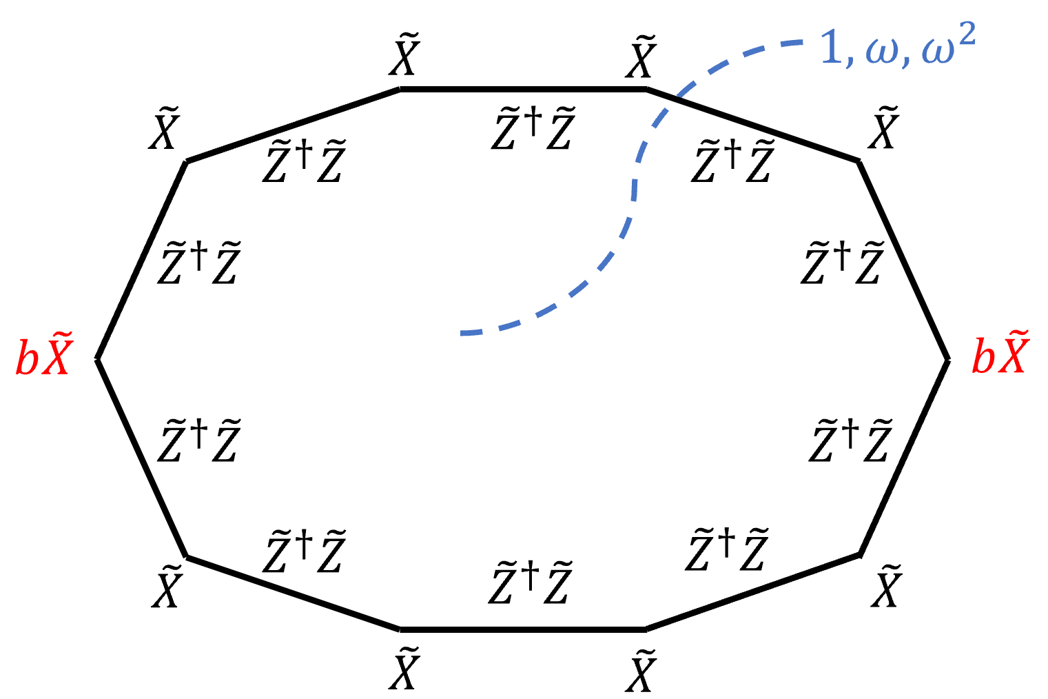
Figure C.8: Our $\mathbb{Z}_{3}^{o}$ gauging and unfolding scheme sends a cluster chain whose endpoints lie on even sites to a Potts chain of this form, with two field-strength defects and a topological twist-sum defect.

C.3 Gauging $\mathbb{Z}^{e}_{3}$ instead

Above we arbitrarily decided to gauge $\mathbb{Z}_{3}^{o}$. We can just as easily gauge $\mathbb{Z}^{e}_{3}$. To map odd-site cluster endpoints to Potts² by gauging $\mathbb{Z}^{e}_{3}$, one can just use the mapping rules of Table 9 and shift cluster site indices by 1. To avoid confusion, throughout this paper we only use the mapping involving gauging $\mathbb{Z}^{o}_{3}$, unless otherwise specified.

C.4 Explicit relation between Potts defects and cluster boundaries

For most practical purposes, the Potts model on a closed loop with some defect insertions is a convenient and familiar system through which we can indirectly deduce the boundary features of the cluster model. However, we also can explicitly relate Potts defects with cluster boundary conditions using the following mapping depicted in Fig. C.9. In summary, the boundary conditions of the cluster model are achieved by fusing the antidiagonal $\mathbb{Z}_{3}$ twist defect to the boundary conditions of Potts². This mapping consists of the following steps:

• The Potts twist defect can be rewritten as the sum of oppositely-oriented twists on both chains. Explicitly on the lattice this may look like a term $\omega^{-a}\tilde{Z}_{j}^{A\dagger}\tilde{Z}_{j+1}^{A}+\omega^{a}\tilde{Z}_{j}^{B\dagger}\tilde{Z}_{j+1}^{B}$ for $a=0,1,2$.

• We interpret this as the sum over $\mathbb{Z}_{3}^{(1,-1)}$ of Potts² group-like topologial defects. Such a sum is the fusion product of orbifold defects $\mathcal{N}_{(1,-1)}$ that implement $\mathbb{Z}_{3}^{(1,-1)}$ gauging (see Eqn.(22)).

• The two orbifold defects can then be moved to either side and fused with the Potts² boundary conditions.

Figure C.9: The boundaries of our physical model of interest, the cluster model, can be understood as the fusion of the boundaries of Potts² with the antidiagonal $\mathbb{Z}_{3}^{(1,-1)}$ orbifold defect. Here we make this connection manifest by showing the exact mapping from the open Potts² chain with boundaries and a twist defect to the orbifolded theory. The twist defect can be rewritten as an antidiagonal twist in the middle of the Potts² chain. The antidiagonal twist can be decomposed into a fusion of antidiagonal orbifold defects, which can then be moved to the boundaries.

Appendix D Analysis of the bond strength defect

Our problem largely reduces to determining the field theory description for the bond-strength defect in the Potts Hamiltonian:

$$\cdots-\tilde{Z}_{-2}\tilde{Z}_{-1}^{\dagger}-\tilde{X}_{-1}-\tilde{Z}_{-1}\tilde{Z}_{0}^{\dagger}-\tilde{X}_{0}-\color[rgb]{1,0,0}b\tilde{Z}_{0}\tilde{Z}_{1}^{\dagger}\color[rgb]{0,0,0}-\tilde{X}_{1}-\tilde{Z}_{1}\tilde{Z}_{2}^{\dagger}-\tilde{X}_{2}-\tilde{Z}_{2}\tilde{Z}_{3}^{\dagger}-\tilde{X}_{3}\cdots+\textrm{h.c.}$$

In this appendix we view this defect in isolation, except in D.2 where we classify boundary conditions of the cluster model. The field theory of the bond-strength defect at the following values of $b$ are exactly known:

• $b=0$: (free, free) factorizing defect ($g=3\sqrt{\frac{5-\sqrt{5}}{30}}=0.91059\ldots$).

• $b=1$: identity defect ($g=1$).

• $b=\infty$: $(A,A)+(B,B)+(C,C)$ factorizing defect ( $g=3\sqrt{\frac{5-\sqrt{5}}{30}}=0.91059\ldots$).

We claim that that these three easily analyzed limits actually characterize our entire range of interest. The proposed phase diagram is shown in Fig. D.10. The claim is the following:

• $0\leq b<1$: (free, free)

• $b=1$: identity

• $1<b$: $(A,A)+(B,B)+(C,C)$

Although we do not have a rigorous analytic proof for this claim, we have various analytic and numeric arguments to support it.

At $b=1$, the local field corresponding to $\tilde{Z}_{0}\tilde{Z}_{1}^{\dagger}+h.c.$ is nothing but $\sim\epsilon_{2/5,2/5}(z,\bar{z})-T_{2,0}(z)-\bar{T}_{0,2}(\bar{z})+\ldots$, whose dominant dimension is $4/5$. So perturbing $b$ away from 1 corresponds to adding a destabilizing relevant defect perturbation $\epsilon(z,\bar{z})$ . It is reasonable to suppose that tuning $b$ to slightly below 1 triggers a flow to the stable defect (no unstable symmetry-allowed perturbations) that exists at $b=0$. Similarly $b$ slightly above 1 triggers a flow to the stable defect at $b=\infty$. Kramers-Wannier duality flips the sign of the relevant defect perturbation $\epsilon(z,\bar{z})$, and likewise it interchanges the $b=0$ and $b=\infty$ limits.

The values of the Affleck-Ludwig defect entropy measure $g$ also support this claim. The $g$-theorem requires that $g$ value is non-increasing in RG flow, which is indeed what takes place in our claim. In fact, $(A,A)+(B,B)+(C,C)$ and $(f,f)$ are the only symmetry-allowed factorizing defects with $g$ value below $1$, and that too only slightly. All other factorizing defects either explicitly break symmetry or have $g$ value more than $1$.

Figure D.10: The conformal defect that arises by changing the strength $b$ of one bond in the Potts model. (a) For $b\geq 0$ there are three different defects in the field theory. At $b=1$ there is no defect (identity defect), which is unstable to local perturbation. Tuning $b$ below or above 1 triggers an RG flow to the stable defects $(\textrm{free},\textrm{free})$ or $\sum_{cyc}(A,A)\equiv(A,A)+(B,B)+(C,C)$ respectively. (b) Conformal defects for complex $b=|b|e^{i\theta}$ computed numerically (colored dots) from long range order (LRO) of cluster order parameters. The blue region in the middle is the (free, free) defect with odd LRO. Red regions are spontaneously fixed defects with even LRO; there are three distinct such defects related by fusion with the $\eta$ topological twist defect ($b\to\omega b$). Purple curves in between refer to the identity defect (or to $\eta$ or $\bar{\eta}$), where both LRO’s vanish.

Numerical results we have obtained, namely the expectation values of order parameters as shown in Fig. 1(d), do strongly agree with this picture. Furthermore, the same defect problem has been identified in the context of Fibonacci anyons in 2+1d systems in Fendley et al. (2009), and the same claim was made.

D.1 Relating even $b>1$ with odd $b<1$

Here we argue numerically and analytically that that the cluster model’s boundary perturbation $b$ on an even endpoint is actually equivalent in some sense (e.g. energy spectrum or operator expectation values) to the boundary perturbation $\frac{\textrm{const}}{b}$ for an $\mathcal{O}(1)$ constant. In the Potts language, this is a relation between the field-strength defect of strength $b$ and the bond-strength defect of strength $\frac{\textrm{const}}{b}$.

Numerically, we see excellent numerical agreement for finite-sized chains at intermediate values of $b$ when computing end-to-end order parameter correlations such as $\langle\tilde{Z}_{0}^{\dagger}\tilde{Z}_{N}\rangle$ (Fig. D.11(b)). We can also analytically study the $b\gg 1$ and $b\approx 1$ limits.

Figure D.11: (a) The field strength defect of strength $b$ is quantitatively similar to the bond strength defect of strength $\tilde{b}$, where $\tilde{b}b$ is on the order of unity. (b) Numerically, we compute the correlation of diametrically-opposite defect-site spins $\tilde{Z}$ in finite closed Potts chains of length $2N$ ($15\leq 2N+1\leq 125$) with bond strength defect (red) of coefficient $b$ (Fig. 3). Likewise we do the same computation but in the presence of a field strength defect (blue) instead (Fig. C.8). We find strong numerical resemblance between bond strength $b$ and field strength $1/b$ for intermediate values of $b$.

D.1.1 $b\gg 1$ and $b\ll 1$

We perform perturbation theory in the large $b$ limit. This quantifies the intuitive observation that $b\to\infty$ is the same as projecting out the associated endpoint. We start with a very general statement about degenerate perturbation theory in a small parameter $\lambda$ and then apply it to our problem.

Generally, consider a Hamiltonian

$$H=-\lambda^{-1}(X+X^{\dagger})+(H_{0}+AZ^{\dagger}+A^{\dagger}Z)$$

for $\lambda\ll 1$, where $X$ and $Z$ are clock matrices acting on one qutrit while $H_{0}$ and $A$ act on an entirely different system ( $[H_{0},X]=[A,X]=0$). We can apply standard degenerate perturbation theory to understand the eigenstates of $\lambda H$. In the unpertrubed ($\lambda=0$) case, $\lambda H|_{\lambda=0}=-(X+X^{\dagger})$ has a collection of degenerate ground states $|1\rangle|n\rangle$ with eigenvalue $-2$ (where $|1\rangle$ is an eigenstate of $X$ with eigenvalue $1$, and $|n\rangle$ is an eigenstate of $H_{0}$ with eigenvalue $h_{n}$), and a collection of excited states $|\omega^{\pm 1}\rangle|n\rangle$ each with energy $+1$. From degenerate perturbation theory we find that to first order in $\lambda$ the states in the $X=1$ sector are modified to

$$|1,n\rangle=|1\rangle|n\rangle+\lambda\sum_{m}\frac{\langle m|A|n\rangle}{(1)-(-2)}\left(-|\omega\rangle|m\rangle+\sum_{\ell\neq n}\frac{\langle\ell|A^{\dagger}|m\rangle}{h_{\ell}-h_{n}}|1\rangle|\ell\rangle\right)+(A\to A^{\dagger},\omega\to\omega^{2})$$

and the corresponding eigenvalues of $\lambda H$ are modified to

$$\lambda E_{n}=-2+\lambda h_{n}+\lambda^{2}\sum_{k}\frac{\langle n|A|k\rangle\langle k|A^{\dagger}|n\rangle}{(-2)-(1)}+\frac{\langle n|A^{\dagger}|k\rangle\langle k|A|n\rangle}{(-2)-(1)}$$

We can replace $\sum_{k}\langle n^{\prime}|A^{\dagger}|k\rangle\langle k|A|n\rangle$ with $\langle n^{\prime}|A^{\dagger}A|n\rangle$. So the eigenstate wave functions projected onto the $X=1$ subspace, and energy (up to an added constant and rescaling by $\lambda$), are in fact those of the Hamiltonian $H_{0}-\frac{1}{3}\lambda(A^{\dagger}A+AA^{\dagger})-2/\lambda$, up to $\mathcal{O}(\lambda^{2})$ corrections.

$$E_{n} =-2/\lambda+h_{n}-\lambda\langle n|\frac{1}{3}(AA^{\dagger}+A^{\dagger}A)|n\rangle$$

$$\langle 1|1,n\rangle =|n\rangle-\lambda\sum_{\ell\neq n}\frac{1}{3}\frac{\langle\ell|A^{\dagger}A+AA^{\dagger}|n\rangle}{h_{n}-h_{\ell}}|\ell\rangle$$

This way, we can argue that for small $\lambda$ we have an effective Hamiltonian:

$$H_{\textrm{eff}}\equiv H_{0}-\frac{1}{3}\lambda(A^{\dagger}A+AA^{\dagger})$$ (26)

For our problem, to understand the defect $\ldots-\tilde{Z}_{-1}\tilde{Z}_{0}^{\dagger}-b\tilde{X}_{0}-\tilde{Z}_{0}\tilde{Z}^{\dagger}_{1}+\ldots+h.c.$, we set $A=-(\tilde{Z}_{-1}+\tilde{Z}_{1})$, $X=\tilde{X}_{0}$, $Z=\tilde{Z}_{0}$ and $b=1/\lambda$. We find that to first order in $1/b$, we can replace the Hamiltonian terms $\ldots-\tilde{Z}_{-1}\tilde{Z}_{0}^{\dagger}-b\tilde{X}_{0}-\tilde{Z}_{0}\tilde{Z}^{\dagger}_{1}+\ldots$ with $\ldots-\frac{2}{3b}\tilde{Z}_{-1}\tilde{Z}_{1}^{\dagger}+\ldots$ (where we ignore the added overall constant).

In conclusion, the cluster model’s even-site termination with perturbation $b\gg 1$ or $b\ll 1$ is quantitatively similar to the adjacent-odd-site termination with perturbation $\frac{2}{3b}$. Namely, energies and wave functions (up to an ancillary qutrit) take similar values.

D.1.2 $b\approx 1$

For $b=1+\delta b\approx 1$ we can use conformal field theory. The small parameter $\delta b$ is the coefficient of the parturbation $\tilde{X}_{0}+\tilde{X}_{0}^{\dagger}\sim\epsilon(z,\bar{z})+\textrm{irrelevant terms}$. KW duality in the field theory turns $\epsilon\to-\epsilon$. Ignoring irrelevant terms, it is the same as $1+\delta b\to 1-\delta b\approx 1/(1+\delta b)$. In the lattice, KW turns the bond strength $1+\delta b$ to the field strength $1+\delta b$. Equating these it follows that $b$ on an even-site endpoint is equivalent to $1/b$ on an odd-site endpoint.

Although there is no consistent constant $k$ such that perturbation strength $b$ on an even endpoint is equivalent to perturbation strength $k/b$ on an odd endpoint for all $b$, generally $k$ is of order unity. Numerical results suggest $k\approx 1$ even for intermediate $b$.

D.2 Summary of boundary conditions

Here we summarize the field theoretic conformal boundary conditions of the cluster model. If the endpoint Hamiltonian looks like $bX_{k}+\sum_{j>k}Z_{j-1}(X_{j}+X_{j}^{\dagger})Z_{j+1}^{\dagger}+h.c.$, Table 10 identifies the conformal boundary condition corresponding to the parity of $k$ and the value of $b$.

	$0\leq b<1$	$b=1$	$b>1$
odd endpoint	$o$-SSB	DQCP	$e$-SSB
even endpoint	$e$-SSB	DQCP	$o$-SSB

Table 10: Conformal boundary conditions of cluster model lattice endpoints

D.3 Comment on Ising bond-strength defect

All Ising conformal defects are known Oshikawa and Affleck (1996, 1997). The main difference from Potts is that Ising has a marginal operator (e.g. $Z_{0}Z_{1}$). Bond strength defects $bZ_{0}Z_{1}$ flow to a continuous family of distinct Dirichlet defects $D(\phi)$ where $\cot{\phi}=b$. The $bZ_{0}Z_{1}\Leftrightarrow\frac{1}{b}X_{0}$ defect equivalence is also exact for all $b$ in the field theory (as well as exact in first-order lattice perturbation theory).

We argue that heuristically we do not expect a $\mathbb{Z}_{2}$ (Ising) generalization of our $\mathbb{Z}_{3}$ (Potts) DQCP result. Gapless boundary deconfined quantum criticality entails a codimension-1 region of parameter space with reduced ground state degeneracy. In contrast the parameter dependence of all the Ising defects suggests the opposite situation. In the presence of one or more of such defects, there may be particular values of $\phi$ which could display increased degeneracy; otherwise the ground state degeneracy would be lower or the same throughout most of parameter space.

D.4 Complex perturbations

We can also consider imaginary $b$ breaking charge-conjugation symmetry. Analytically we predict that the DQCP phenomenon actually persists with complex $b$. This is because near $b=1$, the imaginary perturbation $i(\tilde{Z}_{0}\tilde{Z}_{1}^{\dagger}-h.c.)$ flows to a an irrelevant dimension $9/5$ operator (see Appendix A.2).

Numerically we found the defect phase diagram Fig. D.10. The identity defect persists for a continuous curve of complex values $b_{c}=|b_{c}|e^{i\theta_{c}}$ ( $-\pi/3<\theta_{c}<\pi/3$) where both order parameters vanish simultaneously (see purple curves in Fig. D.10). We also numerically computed energy levels of a closed-loop Potts chain with one bond’s coefficient changed to $b_{c}$ and verified that it matched the defect-less spectrum (Eqn. (8)) in the large $L$ limit. This demonstrates that $b=b_{c}$ is in the same universality as $b=1$.

Appendix E Partition Functions, Energy Levels and Boundary Operator Spectra

Here we apply the defect analysis to determine partition functions of the gapless cluster chain. The partition functions tell us about the low lying energy levels and their degeneracies. Through the state-field correspondence they also tell the spectrum of local boundary operators, their charges and their dimensions, allowing for establishing lattice correspondence.

The gapless cluster chain is remarkably sensitive to whether its length is odd or even. Odd-length left-right-symmetric lattices have the same conformal boundary condition on both sides, whereas even-length chains do not, leading to completely different spectra.

Throughout this appendix, we consistently work in the physical picture of the cluster model on a finite chain. However, when explicitly stated we occasionally refer to the Potts model picture during intermediate steps for derivations. We also use the field theory nomenclature conventions Mong et al. (2014) from the Potts model.

E.1 Odd length chains with same boundary conditions on left and right

In the main text we focused on the odd length case with the same $b$ (i.e., the boundary tuning parameter) on both sides. We summarize the key results in the subsection, before considering the other case in the next subsection.

For $0\leq b<1$, the overall setup in the Potts CFT language looks like two disjoint Potts chains each with free boundary condition on both sides, and the choice of one of three twists on one of the chains. The twist just generates three identical copies. The spectrum is thus given by the following partition function (here we abbreviate $o$-SSB, $e$-SSB, and DQCP boundary conditions as $o$, $e$, and $d$ respectively):

$$\mathcal{Z}_{o,o}=3(\mathcal{Z}_{f,f})^{2}=3(\chi_{I}^{2}+4\chi_{2/3}\chi_{I}+4\chi_{2/3}\chi_{2/3})$$ (27)

The model enjoys a $Vir_{A}\otimes Vir_{B}$ symmetry (in fact, a $\mathcal{W}_{3}^{A}\otimes\mathcal{W}_{3}^{B}$ symmetry), reflected by the partition function’s bilinear form. The low energy Hilbert space splits into three identical $\mathbb{Z}_{3}^{o}$ symmetry broken sectors. The analytically predicted partition function agrees with numerics, as shown in Fig. E.12.

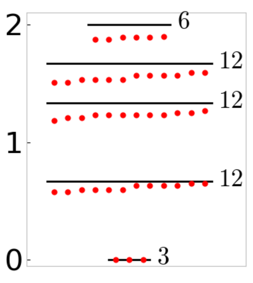
Figure E.12: The first 45 energy levels of the gapless cluster chain with odd length and small boundary perturbations. The vertical axis shows conformal dimensions numerically extracted from the energy levels using (9); they agree with $\mathcal{Z}_{o,o}$ in (27). These values are obtained through DMRG on a chain of length 25 with boundary perturbation $b_{L}=b_{R}=0.1$.

The $b>1$ field theory is related to the $0\leq b<1$ field theory by KW duality (which is an exact unitary map, as mentioned in Appendix C.2.2). Thus, the partition function is the same. Another way to see this is that overall setup in the Potts language is that of aligned spontaneously fixed spins on either defect, and a twist insertion that mis-aligns one of the defects. Thus the partition function is

$$\mathcal{Z}_{e,e}=3(\mathcal{Z}_{A,A+B+C})^{2}=3(\chi_{I}^{2}+4\chi_{2/3}\chi_{I}+4\chi_{2/3}\chi_{2/3})$$ (28)

In both cases, the overall factor of 3 reflects spontaneous breaking of $\mathbb{Z}_{3}^{o}$ or $\mathbb{Z}_{3}^{e}$. For example, in the $e$-SSB case, there is an identical spectrum for each choice of spin $A$, $B$, or $C$ on one defect; this choice indicates spontaneous selection of a vacuum expectation value for the $\mathbb{Z}^{e}_{3}$ order parameter. The CFT for each of the vacua is also endowed with the unbroken $\mathbb{Z}_{3}$ subgroup’s symmetry.

For $b=1$, the overall setup is even simpler in the Potts language. The system can be thought of as a single Potts chain with three choices of twist. The partition function is thus

$$\mathcal{Z}_{d,d}=\mathcal{Z}_{1}+\mathcal{Z}_{\eta}+\mathcal{Z}_{\eta^{2}}=|\chi_{I}+2\chi_{2/3}|^{2}+|\chi_{\epsilon}+2\chi_{1/15}|^{2}$$ (29)

We have introduced the notation of complex conjugation to reflect the enhanced $Vir\otimes\overline{Vir}$ symmetry. This spectrum is manifestly nondegenerate as there is only one ground state, counted here in $|\chi_{I}|^{2}$. The field theory enjoys the full $\mathbb{Z}^{o}_{3}\otimes\mathbb{Z}^{e}_{3}$ symmetry.

E.2 Even length chains with different boundary conditions on left and right

We can repeat the construction in Appendix C.2 for a cluster chain with even length on sites $1\leq j\leq 2N$.

$$-H=b_{L}X_{1}+b_{R}X_{2N}+h.c.+\sum_{j=2}^{2N-1}(X_{j}+h.c.)(Z_{j-1}Z_{j+1}^{\dagger}+h.c.)$$

We find the model maps to a closed Potts chain of length $2N-1$ with the bond strength defect on one side, the field strength defect on the other side, and three twist options (Fig. E.13). For generic $b_{L}=b_{R}\neq 1$, the left and right boundary conditions look different. This has major consequences on the spectrum and finite size splitting.

Figure E.13: The cluster model on an even length chain with boundary perturbations $b_{L}X_{1}$ and $b_{R}X_{2N}$ can be mapped to a Potts chain with defects and symmetry twists as shown.

For $b_{L}=b_{R}\neq 1$, the ground states are actually not three-fold degenerate, like in the odd length case, but nine-fold degenerate. For $b_{L}=b_{R}<1$ the partition function is

$$\mathcal{Z}_{o,e}(q)=(\mathcal{Z}_{f,A+B+C})^{2}=9(\chi_{1/8}+\chi_{13/8})^{2}$$ (30)

The ground states have conformal dimension $1/4$ instead of $0$. The spectrum is shown in Fig. E.14(a).

Figure E.14: Numerical results for the energy levels of the gapless cluster chain with even length and small boundary perturbations. (a) The first 72 energy levels with length $L=20$ and boundary perturbations $b_{L}=b_{R}=1$, plotted analogously to Fig. E.12. The conformal ground state has ninefold degeneracy (instead of threefold) and dimension $1/4$ (instead of $0$). (b) For even length systems, the finite size splitting is a first order effect in the boundary perturbation, separating some of the nine ground states in proportion to $L^{-4/3}$.

We can also consider the finite size splitting between the ground states. Interestingly it is first-order in $b$ and scales $\propto{L^{-4/3}}$ (Fig. E.14(b)). For $b_{L},b_{R}\ll 1$, the nine lowest energy levels $E_{k,\ell}$ are given by $E_{k,\ell}-E_{0}\propto\textrm{Re}(-b_{L}\omega^{k}-b_{R}\omega^{\ell})L^{-4/3}$ for some integer labels $1\leq k,\ell\leq 3$ and a non-universal constant $E_{0}$. The $L^{-4/3}$ scaling, derived through dimensional analysis, suggests edge modes are less strongly algebraically localized than in the odd length case, where splitting is second-order and $\propto{L^{-5/3}}$.

The $b_{L}=b_{R}>1$ case is KW dual to $b_{L}=b_{R}<1$ and both have the same nine-fold degenerate spectrum $\mathcal{Z}_{o,e}=\mathcal{Z}_{e,o}$. When $b_{L}=b_{R}=1$, the even-length model just like the odd-length model is at a DQCP with spectrum $\mathcal{Z}_{d,d}$, where edge modes dissolve and Potts description has no localized defects.

E.3 Summary of spectral properties for left and right boundary conditions

We can also consider $b_{L}\neq b_{R}$ for any chain length. Generally, one can match a value of $b$ on an endpoint to a cluster model conformal boundary condition as per Table 10. Then one can deduce the partition function, energy levels, and degeneracy as per Tables 11 and 12.

	Right $o$-SSB	Right DQCP	Right $e$-SSB
Left $o$-SSB	3	3	9
Left DQCP	3	1	3
Left $e$-SSB	9	3	3

Table 11: Degeneracies of the conformal ground state for different combinations of left and right boundary conditions.

	Right $o$-SSB	Right DQCP	Right $e$-SSB
Left $o$-SSB	$3(\mathcal{Z}_{ff}(q))^{2}$	$3\mathcal{Z}_{ff}(\sqrt{q})$	$9(\mathcal{Z}_{fA}(q))^{2}$
Left DQCP	$3\mathcal{Z}_{ff}(\sqrt{q})$	$\mathcal{Z}_{1+\eta+\eta^{2}}(q)$	$3\mathcal{Z}_{ff}(\sqrt{q})$
Left $e$-SSB	$9(\mathcal{Z}_{fA}(q))^{2}$	$3\mathcal{Z}_{ff}(\sqrt{q})$	$3(\mathcal{Z}_{ff}(q))^{2}$

Table 12: Finite temperature partition functions for different combinations of left and right boundary conditions. Here, $\mathcal{Z}_{ff}=\chi_{I}+2\chi_{2/3}$ and $\mathcal{Z}_{fA}=\chi_{1/8}+\chi_{13/8}$. The variable $q=e^{-2\pi\beta/L}$ in all cases.

E.4 Symmetry-resolved energy spectra and boundary operators

We can organize energy levels in $\mathcal{Z}_{x,x}$ for $x=o,e,d$ according to their eigenvalues under the generators of the $\mathbb{Z}_{3}^{o}\times\mathbb{Z}_{3}^{e}$ symmetry. This also tells us the symmetry charges of local boundary operators which couple these distinct levels or sectors.

There is a subtlety for boundary SSB of a symmetry $G$. Any degenerate Hamiltonian’s eigenstates can be expressed as simultaneous eigenstates of $G$ generators. In fact with finite-size energy splittings, those are the exact energy eigenstates. But such $G$-invariant states may be macroscopically entangled. In the infinite-size / CFT limit the more physical basis may be one of $G$-breaking states, each in an equal-weight superposition of $G$ charges. In our boundary SSB scenarios, the Hilbert space breaks up into 9 superselection sectors corresponding to spontaneous choices of boundary condition on the left and right, of which three superselection sectors contain a distinct CFT vacuum. The superselection sectors lack a well-defined $G$ charge.

E.4.1 $o$-SSB

We can classify the 27 terms in $\mathcal{Z}_{o,o}$ into symmetry-resolved eigenspaces of $U^{e}$ and $U^{o}$ generators as in Table 13. Our notation $\chi_{\psi^{A/B(\dagger)}}\equiv\chi_{2/3}$ explicitly denotes $\mathcal{W}_{3}^{A}\otimes\mathcal{W}_{3}^{B}$-primary local boundary operators. $\psi^{A/B}$ and $\psi^{A/B\dagger}$ are local boundary operators with $\mathbb{Z}_{3}^{e}$ charge $\omega$ and $\omega^{*}$ respectively (not to be confused with Potts² bulk operators).

$$\mathcal{Z}_{o,o}=3(\chi_{I}+\chi_{2/3}+\chi_{2/3})^{2}$$

	$U^{e}=1$	$U^{e}=\omega$	$U^{e}=\omega^{2}$
$U^{o}=1$	$\chi_{I}\chi_{I}+\chi_{\psi^{A}}\chi_{\psi^{B\dagger}}+\chi_{\psi^{A\dagger}}\chi_{\psi^{B}}$	$\chi_{I}\chi_{\psi^{B}}+\chi_{\psi^{A}}\chi_{I}+\chi_{\psi^{A\dagger}}\chi_{\psi^{B\dagger}}$	$\chi_{I}\chi_{\psi^{B\dagger}}+\chi_{\psi^{A\dagger}}\chi_{I}+\chi_{\psi^{A}}\chi_{\psi^{B}}$
$U^{o}=\omega$	$\chi_{I}\chi_{I}+\chi_{\psi^{A}}\chi_{\psi^{B\dagger}}+\chi_{\psi^{A\dagger}}\chi_{\psi^{B}}$	$\chi_{I}\chi_{\psi^{B}}+\chi_{\psi^{A}}\chi_{I}+\chi_{\psi^{A\dagger}}\chi_{\psi^{B\dagger}}$	$\chi_{I}\chi_{\psi^{B\dagger}}+\chi_{\psi^{A\dagger}}\chi_{I}+\chi_{\psi^{A}}\chi_{\psi^{B}}$
$U^{o}=\omega^{2}$	$\chi_{I}\chi_{I}+\chi_{\psi^{A}}\chi_{\psi^{B\dagger}}+\chi_{\psi^{A\dagger}}\chi_{\psi^{B}}$	$\chi_{I}\chi_{\psi^{B}}+\chi_{\psi^{A}}\chi_{I}+\chi_{\psi^{A\dagger}}\chi_{\psi^{B\dagger}}$	$\chi_{I}\chi_{\psi^{B\dagger}}+\chi_{\psi^{A\dagger}}\chi_{I}+\chi_{\psi^{A}}\chi_{\psi^{B}}$

Table 13: $\mathbb{Z}^{e}_{3}\times\mathbb{Z}^{o}_{3}$ symmetry resolution of local boundary operator content of $o$-SSB boundary condition

Here $\mathbb{Z}_{3}^{o}$ is spontaneously broken. Thus technically all operators lack a well-defined $U^{o}$ charge, despite what it naively looks like in the table. Instead, operators and states in each superselection sector are in some equal-weight linear combination of the three identical rows in this table. The operators $\psi^{A}$, $\psi^{B\dagger}$, and $\psi^{A\dagger}\psi^{B}$ are the boundary-condition-changing operators that toggle in the same way from one spontaneous choice of boundary to another; they (and their conjugate versions) are what we call the boundary disorder operators.

E.4.2 $e$-SSB

The symmetry resolution for the $e$-SSB is the same as that for the $o$-SSB but with $e\Leftrightarrow o$ (Table 14). Here $\psi^{A/B}$ and $\psi^{A/B\dagger}$ refer to local boundary operators with $\mathbb{Z}_{3}^{o}$ charge $\omega$ and $\omega^{*}$ respectively.

	$U^{e}=1$	$U^{e}=\omega$	$U^{e}=\omega^{2}$
$U^{o}=1$	$\chi_{I}\chi_{I}+\chi_{\psi^{A}}\chi_{\psi^{B\dagger}}+\chi_{\psi^{A\dagger}}\chi_{\psi^{B}}$	$\chi_{I}\chi_{I}+\chi_{\psi^{A}}\chi_{\psi^{B\dagger}}+\chi_{\psi^{A\dagger}}\chi_{\psi^{B}}$	$\chi_{I}\chi_{I}+\chi_{\psi^{A}}\chi_{\psi^{B\dagger}}+\chi_{\psi^{A\dagger}}\chi_{\psi^{B}}$
$U^{o}=\omega$	$\chi_{I}\chi_{\psi^{B}}+\chi_{\psi^{A}}\chi_{I}+\chi_{\psi^{A\dagger}}\chi_{\psi^{B\dagger}}$	$\chi_{I}\chi_{\psi^{B}}+\chi_{\psi^{A}}\chi_{I}+\chi_{\psi^{A\dagger}}\chi_{\psi^{B\dagger}}$	$\chi_{I}\chi_{\psi^{B}}+\chi_{\psi^{A}}\chi_{I}+\chi_{\psi^{A\dagger}}\chi_{\psi^{B\dagger}}$
$U^{o}=\omega^{2}$	$\chi_{I}\chi_{\psi^{B\dagger}}+\chi_{\psi^{A\dagger}}\chi_{I}+\chi_{\psi^{A}}\chi_{\psi^{B}}$	$\chi_{I}\chi_{\psi^{B\dagger}}+\chi_{\psi^{A\dagger}}\chi_{I}+\chi_{\psi^{A}}\chi_{\psi^{B}}$	$\chi_{I}\chi_{\psi^{B\dagger}}+\chi_{\psi^{A\dagger}}\chi_{I}+\chi_{\psi^{A}}\chi_{\psi^{B}}$

Table 14: $\mathbb{Z}^{e}_{3}\times\mathbb{Z}^{o}_{3}$ symmetry resolution of local boundary operator content of $e$-SSB boundary condition

E.4.3 DQCP

Finally we can resolve the states at the DQCP into their respective symmetry sectors (Table 15).

$$\mathcal{Z}_{d,d}=|\chi_{I}+\chi_{\psi}+\chi_{\psi^{\dagger}}|^{2}+|\chi_{\epsilon}+\chi_{\sigma}+\chi_{\sigma^{\dagger}}|^{2}$$

	$U^{e}=1$	$U^{e}=\omega$	$U^{e}=\omega^{2}$
$U^{o}=1$	$|\chi_{I}|^{2}+|\chi_{\epsilon}|^{2}$	$\chi_{\sigma}\bar{\chi}_{\sigma}+\chi_{\psi}\bar{\chi}_{\psi}$	$\chi_{\sigma^{\dagger}}\bar{\chi}_{\sigma^{\dagger}}+\chi_{\psi^{\dagger}}\bar{\chi}_{\psi^{\dagger}}$
$U^{o}=\omega$	$\chi_{\sigma^{\dagger}}\bar{\chi}_{\sigma}+\chi_{\psi^{\dagger}}\bar{\chi}_{\psi}$	$\chi_{\epsilon}\bar{\chi}_{\sigma^{\dagger}}+\chi_{I}\bar{\chi}_{\psi^{\dagger}}$	$\chi_{\sigma}\bar{\chi}_{\epsilon}+\chi_{\psi}\bar{\chi}_{I}$
$U^{o}=\omega^{2}$	$\chi_{\sigma}\bar{\chi}_{\sigma^{\dagger}}+\chi_{\psi}\bar{\chi}_{\psi^{\dagger}}$	$\chi_{\sigma^{\dagger}}\bar{\chi}_{\epsilon}+\chi_{\psi^{\dagger}}\bar{\chi}_{I}$	$\chi_{\epsilon}\bar{\chi}_{\sigma}+\chi_{I}\bar{\chi}_{\psi}$

Table 15: $\mathbb{Z}^{e}_{3}\times\mathbb{Z}^{o}_{3}$ symmetry resolution of local boundary operator content of DQCP boundary condition.

Here our choice of notation for local boundary fields at the DQCP makes manifest their correspondence to the Potts models’ bulk fields (including $\mathbb{Z}_{3}$ twist fields) using the naming conventions of Mong et al. (2014). Although at the DQCP $\mathbb{Z}_{3}^{e}$ and $\mathbb{Z}_{3}^{o}$ are on an equal footing, it is intuitive to picture the system as translation-invariant Potts¹ model on a closed loop by gauging a $\mathbb{Z}_{3}$ subgroup ($\mathbb{Z}^{o}_{3}$ without loss of generality). In this Potts¹ picture, the aforementioned bulk-boundary correspondence is just given by translation.

E.5 Lattice-BCFT correspondence

In Verresen et al. (2021), the bulk twist operators played an important role in the boundary physics upon being dragged to the boundary. Here we build upon this concept for our model. We discuss the dominant charged and uncharged boundary operators in the above three boundary conditions, which will elucidate the connection between boundary disorder operators and the vortex condensation picture of DQCP.

Bulk twist operator	Dimension	$\mathbb{Z}^{e}_{3}$ charge	$\mathbb{Z}^{o}_{3}$ charge	Potts2 CFT form	Boundary version
$\big{(}\prod_{k\leq j}X_{2k-1}\big{)}Z_{2j}$	2/15	$\omega$	1	$\sigma^{A}(z,\bar{z})$	$X_{1}Z_{2}$
$\big{(}\prod_{k\leq j}X_{2k}\big{)}Z_{2j+1}$	2/15	1	$\omega$	$\mu^{A\dagger}(z,\bar{z})$	$Z_{1}$
$\prod_{k\leq j}X_{2k-1}$	4/15	1	1	$\sigma^{A\dagger}(z,\bar{z})\sigma^{B}(z,\bar{z})$	$X_{1}$
$\prod_{k\leq j}X_{2k}$	4/15	1	1	$\mu^{A}(z,\bar{z})\mu^{B}(z,\bar{z})$	$X_{2}$

Table 16: The $\mathbb{Z}_{3}\times\mathbb{Z}_{3}$ twist operators of the cluster model

We are especially interested the lattice-field correspondence for local boundary fields obtained by dragging bulk nonlocal $\mathbb{Z}_{3}\times\mathbb{Z}_{3}$-twist operators to the boundary. They play important roles as order parameters (charged operators with nonzero long-range-order to indicate boundary SSB) and disorder operators (operators that toggle between boundary spontaneous superselection sectors). Generally we expect the same twist operator dragged to different near-boundary sites (e.g. $Z_{1}$ and $X_{2}Z_{3}$ and $X_{2}X_{4}Z_{5}$) should have the same qualitative field theory description.

E.5.1 $o$-SSB Boundary condition

The boundary operator $Z_{1}$ is $\mathbb{Z}_{3}^{e}$ neutral and thus belongs to $\chi_{I}\chi_{I}+\chi_{\psi^{A}}\chi_{\psi^{B\dagger}}+\chi_{\psi^{A\dagger}}\chi_{\psi^{B}}$. Since it flows to the identity operator while also being $\mathbb{Z}_{3}^{o}$-charged, it plays the role of boundary order parameter.

The boundary operator $X_{1}Z_{2}$ is $\mathbb{Z}_{3}^{e}$ charged, thus belonging to $\chi_{I}\chi_{\psi^{B}}+\chi_{\psi^{A}}\chi_{I}+\chi_{\psi^{A\dagger}}\chi_{\psi^{B\dagger}}$. At $b=0$, $X_{1}Z_{2}$ flows exactly to $\psi^{A}$ and its descendants and thus plays the role of a relevant boundary disorder operator. At nonzero $b$, it has overlap with the oppositely-toggling boundary disorder operator $\psi^{B}$ and the non-toggling operator $\psi^{A\dagger}\psi^{B\dagger}$, but nevertheless a dressed version of it may be regarded as a relevant boundary disorder operator. It is the 0+1D analog of the charged vortex excitation operator. As a Hamiltonian perturbation (violating the $\mathbb{Z}_{3}\times\mathbb{Z}_{3}$ symmetry), it could destabilize the boundary condition into a stable non-degenerate symmetry-preserving one.

Neutral boundary operators $X_{1},X_{2}$ belong to $\chi_{I}\chi_{I}+\chi_{\psi^{A}}\chi_{\psi^{B\dagger}}+\chi_{\psi^{A\dagger}}\chi_{\psi^{B}}$. Their leading non-constant contributions have dimension $4/3$. Thus, symmetry-allowed perturbations are irrelevant despite coupling different edge modes. This analysis rigorously agrees with our rough intuitive prediction that upon dragging to the boundary, the lighter bulk twist operators (e.g. $\mu^{A}(z,\bar{z})$) turn into lighter boundary operators (e.g. $\psi^{A}$) whereas the heavier bulk twist operators (e.g. $\mu^{A}(z,\bar{z})\mu^{B\dagger}(z,\bar{z})$) turn into the heavier (and thus irrelevant) boundary operators (e.g. $\psi^{A}\psi^{B\dagger}$) .

E.5.2 $e$-SSB Boundary condition

The $e$-SSB boundary condition is Kramers Wannier dual to the $o$-SSB boundary condition. So, we can immediately conclude from the previous subsection that $X_{1}Z_{2}$ is a boundary order parameter, $X_{2}Z_{3}$ (or $Z_{1}$ for finite $b$) is a relevant boundary disorder operator, and $X_{1}$ and $X_{2}$ are irrelevant neutral boundary operators. The boundary order parameter and the relevant boundary disorder operator interchange roles between $o$-SSB and $e$-SSB. This demonstrates that condensing of the relevant boundary disorder operator drives the boundary phase transition.

E.5.3 DQCP

At the DQCP there is no SSB and hence no order parameter or toggling disorder operator. Charged boundary operators have a different interesting interpretation. The aforementioned emergent bulk-boundary symmetry exactly identifies charged bulk twist operators in Table 16 with their boundary versions. Thus as $b\to 1$, the SSB boundary order parameters $X_{1}Z_{2}$ and $Z_{1}$ both turn into dimension-$2/15$ fields that can be identified with bulk Potts order/disorder operators $\sigma$ and $\mu$. Thus, edge order parameters manifestly disappear and furthermore the Potts KW duality ($\sigma\Leftrightarrow\mu$) acts as a DQCP symmetry enhancement exchanging the order parameters of the two nearby boundary SSB phases. Meanwhile neutral operators $X_{1}$ and $X_{2}$ belong to $\chi_{I}\bar{\chi}_{I}+\chi_{\epsilon}\bar{\chi}_{\epsilon}$. Their dominant non-identity contribution is of dimension $4/5$, making them relevant destabilizing perturbations, pushing us into one of the two above boundary SSB phases.

Appendix F Boundary State Analysis

In Appendix E we worked out the properties of the $o$-SSB, $e$-SSB, and DQCP boundary conditions indirectly by considering the Potts model. In this appendix we take an alternative more direct approach by explicitly writing out these cluster boundary conditions through the boundary state formalism (see B.7 for a review). Here we largely reproduce results of Appendix E, but with the advantage that the boundary state formalism allows us to write these boundary conditions in terms of known quantities (i.e. in terms of a bulk Hilbert space) instead of merely treating them like abstract labels.

Here we will use the direct mapping from Appendix C.4 to determine the boundary states of the three boundary conditions. We start with the boundary state formalism for the boundary conditions of Potts². Then we will apply an orbifold of the antidiagonal $\mathbb{Z}_{3}$ symmetry to this model to obtain the boundary states for free orbifolded boundary conditions. The Potts² boundaries we consider are the following (here subscripts $A$ and $B$ label the two chains, and for brevity we abbreviate $|{\rm fixed}-\omega^{a}\rangle$ as $|\omega^{a}\rangle$ and omit the tensor product symbol $\otimes$ between chains $A$ and $B$.):

• free on both chains, $|{\rm free}\rangle_{A}|{\rm free}\rangle_{B}$

• spontaneously fixed aligned on both chains, $\sum_{a=0}^{2}|\omega^{a}\rangle_{A}|\omega^{a}\rangle_{B}$

• fold of identity defect (the boundary created by taking a singe Potts chain and folding it)

By directly applying the formulas from section B.6, the free² boundary state is given by

$$|{\rm free}\rangle_{A}|{\rm free}\rangle_{B}=3N^{2}\left(|0\rangle\rangle-|3\rangle\rangle-\sqrt{\varphi}|2/5\rangle\rangle+\sqrt{\varphi}|7/5\rangle\rangle\right)_{A}\left(|0\rangle\rangle-|3\rangle\rangle-\sqrt{\varphi}|2/5\rangle\rangle+\sqrt{\varphi}|7/5\rangle\rangle\right)_{B}$$

The spontaneously fixed aligned boundary condition is

$$\begin{split}\sum_{a=0}^{2}|\omega^{a}\rangle_{A}|\omega^{a}\rangle_{B}=&3N^{2}\left(|I\rangle\rangle+\sqrt{\varphi}|\epsilon\rangle\rangle\right)_{A}\left(|I\rangle\rangle+\sqrt{\varphi}|\epsilon\rangle\rangle\right)_{B}\\ &+3N^{2}\left(|\psi\rangle\rangle+\sqrt{\varphi}|\sigma\rangle\rangle\right)_{A}\left(|\psi^{\dagger}\rangle\rangle+\sqrt{\varphi}|\sigma\rangle\rangle\right)_{B}\\ &+3N^{2}\left(|I\rangle\rangle+\sqrt{\varphi}|\epsilon\rangle\rangle\right)_{A}\left(|I\rangle\rangle+\sqrt{\varphi}|\epsilon\rangle\rangle\right)_{B}\end{split}$$

Finally the fold boundary condition cannot be expressed as a sum of some tensor products of Potts Ishibashi states, but it can be found by applying the folding trick (heuristically, $(|a\rangle\langle b|\to|a\rangle_{A}|b\rangle_{B}$) to turn the identity operator into a boundary condition.

$$|\textrm{fold}\rangle=\sum_{h}\sum_{J}|h,J\rangle_{A}|h,J\rangle_{B}$$

where here $h$ refers to each Potts¹ bulk $\mathcal{W}_{3}\otimes\overline{\mathcal{W}}_{3}$-primary operator and $J$ schematically refers to its $\mathcal{W}_{3}$ descendants. All we have done is taken the identity operator and folded it.

Now we apply the antidiagonal orbifold, which entails simply multiplying by the $\mathbb{Z}^{(1,-1)}_{3}$ orbifold defect:

$$\mathcal{N}_{(1,-1)}=\frac{1}{\sqrt{3}}\left(1+\eta_{A}\bar{\eta}_{B}+\bar{\eta}_{A}\eta_{B}\right)$$

This results in the following boundary conditions of the orbifolded theory:

$$\begin{split}|\textrm{o-ssb}\rangle&=\mathcal{N}_{(1,-1)}|\textrm{free}\rangle_{A}|\textrm{free}\rangle_{B}=\sqrt{3}|\textrm{free}\rangle_{A}|\textrm{free}\rangle_{B}\\ &=3\sqrt{3}N^{2}\left(|0\rangle\rangle-|3\rangle\rangle-\sqrt{\varphi}|2/5\rangle\rangle+\sqrt{\varphi}|7/5\rangle\rangle\right)_{A}\left(|0\rangle\rangle-|3\rangle\rangle-\sqrt{\varphi}|2/5\rangle\rangle+\sqrt{\varphi}|7/5\rangle\rangle\right)_{B}\\ |\textrm{e-ssb}\rangle&=\mathcal{N}_{(1,-1)}\sum_{m}|\omega^{m}\rangle_{A}|\omega^{m}\rangle_{B}=\frac{1}{\sqrt{3}}\sum_{m,n}|\omega^{m}\rangle_{A}|\omega^{n}\rangle_{B}\\ &=3\sqrt{3}N^{2}\left(|0\rangle\rangle+|3\rangle\rangle+\sqrt{\varphi}|2/5\rangle\rangle+\sqrt{\varphi}|7/5\rangle\rangle\right)_{A}\left(|0\rangle\rangle+|3\rangle\rangle+\sqrt{\varphi}|2/5\rangle\rangle+\sqrt{\varphi}|7/5\rangle\rangle\right)_{B}\\ \end{split}$$ (31)

Note that $|\textrm{e-ssb}\rangle$ and $|\textrm{e-ssb}\rangle$ have very similar forms; indeed they are related to each other by the transformation $\mathcal{K}$ from Eqn. (24) which looks like Kramers-Wannier duality on the closed Potts chain.

The fold boundary gauges to give the DQCP boundary. Each term $|h,J\rangle_{A}|h,J\rangle_{B}$ is invariant under antidiagonal generator $\eta_{A}\bar{\eta}_{B}$. Thus,

$$\begin{split}|\textrm{DQCP}\rangle&=\mathcal{N}_{(1,-1)}\sum_{h}\sum_{J}|h,J\rangle_{A}|h,J\rangle_{B}\\ &=\sqrt{3}\sum_{h}\sum_{J}|h,J\rangle_{A}|h,J\rangle_{B}\\ \end{split}$$ (32)

Note that although we have written these cluster boundary states in the language of the Potts² bulk Hilbert space $\mathcal{H}_{\textrm{Potts}^{2}}=\mathcal{H}_{\textrm{Potts }A}\otimes\mathcal{H}_{\textrm{Potts }B}$, they actually live in the cluster model’s bulk Hilbert space $\mathcal{H}_{cluster}$. The cluster model’s bulk Hilbert space is a direct sum of the $\mathbb{Z}_{3}^{(1,-1)}$-symmetric subspace of $\mathcal{H}_{\textrm{Potts}^{2}}$ and of the ($\mathbb{Z}_{3}^{(1,-1)}$-symmetric subspaces of) $\mathbb{Z}_{3}^{(1,-1)}$-twisted sectors of the Potts Hilbert space. It is only because these three boundary states are invariant under $\mathbb{Z}_{3}^{o}$ that we can conveniently write them in terms of just $\mathcal{H}_{\textrm{Potts}^{2}}$ states.

It is not immediately obvious here as written that the states $|\textrm{e-ssb}\rangle$ and $|\textrm{o-ssb}\rangle$ are the sum of three simple boundary conditions and that $|\textrm{DQCP}\rangle$ is itself a simple boundary condition. However, we can deduce this from the partition function with the same boundary condition on both sides. We can write down partition functions in terms of these states in terms of $\tilde{q}=\exp(-2\pi L/\beta)$ using the fact that $\langle\langle\phi_{i}|\tilde{q}^{L_{0}-c/24}|\phi_{j}\rangle\rangle=\delta_{ij}\chi_{i}(\tilde{q})$, and then apply a modular transformation to obtain the coefficient of $\chi_{0}(q)$ which tells us the number of simple boundary conditions into which a compound boundary condition decomposes. Going through this procedure, we can recover all the partition functions from Appendix E.

Furthermore for each spontaneous symmetry breaking boundary conditions we can in fact write down the boundary states for the three simple boundary conditions into which it decomposes. For simplicity we write them only for $|\textrm{e-ssb}\rangle$; that way we do not need to introduce new notation for Potts² twisted sector states.

$$|\textrm{e-ssb}\rangle =\sum_{a=0}^{2}|\textrm{e-}a\rangle$$ (33)

$$|\textrm{e-}a\rangle =\frac{1}{\sqrt{3}}\sum_{b=0}^{2}|\omega^{a+b}\rangle_{A}|\omega^{a-b}\rangle_{B}$$ (34)

Each one manifestly breaks the $\mathbb{Z}^{e}_{3}$ symmetry as we would expect; $\eta_{A}\eta_{B}|\textrm{e-}a\rangle=|\textrm{e-}(a+1)\rangle$. Their partition functions are given (for $a\neq a^{\prime}$) by:

$$\mathcal{Z}_{e-a,e-a} =\chi_{I}(q)^{2}+2\chi_{2/3}(q)^{2}$$ (35)

$$\mathcal{Z}_{e-a,e-a^{\prime}} =\chi_{2/3}(q)^{2}+2\chi_{2/3}(q)\chi_{I}(q)$$ (36)

Appendix G Ising^2⋆

Here we consider an interesting non-example of boundary DQCP, but which looked like a promising direction at first. Let us consider two decoupled critical Ising chains, a theory we will just call Ising², with $G=\mathbb{Z}_{2}^{A}\times\mathbb{Z}_{2}^{B}$ global symmetry given by the usual spin flip symmetries in each chain, which we have denoted $A$ and $B$. The nearby phase diagram of this theory consists of the trivial phase, $A$-SSB and $B$-SSB phases, and complete SSB phase.

If we apply the $\mathbb{Z}_{2}\times\mathbb{Z}_{2}$ cluster entangler, or equivalently add a decoupled cluster chain and take $G$ to act diagonally between it and the Ising² chain, then we get a theory Ising^2⋆ which has the same spectrum of local operators but instead of the trivial phase appearing in its nearby phase diagram (upon disordering both Ising chains), the cluster SPT phase appears instead. There is no nearby trivial phase.

Moreover, if we study the $\mathbb{Z}_{2}^{A}$ twisted sector of Ising², we find it has a unique lightest operator, which is the disorder operator of the $A$-chain $\mu_{A}$ times the identity operator $1_{B}$ of the $B$ chain. This operator is $G$-neutral. However, for Ising^2⋆, it gets decorated by the SPT $\mathbb{Z}_{2}^{A}$-string operator, and becomes $\mathbb{Z}_{2}^{B}$-odd. Ising² and Ising^2⋆ thus appear to be distinct gapless SPTs, distinguished by their bulk invariants.

However, as noted in Verresen et al. (2021), there is a continuous path connecting Ising² and Ising^2⋆, that is, an exactly marginal deformation from one into the other, along which there are no phase transitions. What happens is that the along this deformation, say starting from Ising^2⋆ the neutral $\mathbb{Z}_{2}^{A}$-string operator $\mathcal{O}_{1}=\mu_{A}1_{B}$ is getting heavier while the $\mathbb{Z}_{2}^{B}$-odd such operator $\mathcal{O}_{2}=\mu_{A}\sigma_{B}$ is becoming lighter (note the theory no longer splits as a product along this path, which is tuned by the energy-energy coupling between the chains). At a KT transition, they are degenerate and the above bulk topological ‘invariant’ becomes ill-defined. Then they cross and $\mathcal{O}_{2}$ is the lighter one, eventually becoming $\mu_{A}^{\prime}1_{B}^{\prime}$ at Ising^2⋆ once we reach the T-dual value of the marginal parameter (i.e., the $c=1$ orbifold radius).

This suggests that Ising^2⋆, despite its non-trivial bulk invariant, has a trivial symmetric boundary. Intuitively we can tune the marginal parameter near the boundary towards Ising², which does have a symmetric trivial boundary, namely the $|{\rm free}\rangle\otimes|{\rm free}\rangle$ boundary. Let us see what this looks like in detail.

We can think of the open boundary condition for an uncoupled Ising² and cluster chain as a $|{\rm free}\rangle\otimes|{\rm free}\rangle$ boundary with a decoupled qubit carrying a projective doublet under the symmetry, with $\mathbb{Z}_{2}^{A}$ acting as $X_{\partial}$ and $\mathbb{Z}_{2}^{B}$ acting as $Z_{\partial}$.

There are two symmetric relevant boundary couplings, namely $g_{A}\sigma_{A}Z_{\partial}$ and $g_{B}\sigma_{B}X_{\partial}$, where $\sigma_{A,B}$ denotes the boundary order parameter of the $A$ or $B$ chain. If we add just one, say $g_{A}$, then we flow to the $|{\rm spontfix}\rangle\otimes|{\rm free}\rangle$ boundary, which spontaneously breaks $\mathbb{Z}_{2}^{A}$ (i.e., we effectively obtain a fixed boundary condition for each sector $X_{\partial}=\pm 1$), and vice versa. We might try to look for a DQCP between these two boundaries, but in fact they are just unstable. If we look again at $g_{B}$ in the $|{\rm spontfix}\rangle\otimes|{\rm free}\rangle$ boundary, we see it is $\mu_{A}\sigma_{B}$, where $\mu_{A}$ is the boundary disorder operator of the $A$ chain, due to $X_{\partial}$ toggling the eigenvalue of $Z_{\partial}$. This operator is marginal, in fact exactly marginal, as we can see when mapping to the orbifold variables.

Ising² can be described as a $\mathbb{Z}_{2}$ orbifold of a compact boson at the free fermion radius Ginsparg (1990). The boundary states we need are given in Oshikawa and Affleck (1996, 1997) (the free fermion radius is $r=1$ in their notation). The theory is given in terms of two dual fields $\varphi$, $\theta$, both $2\pi$ periodic (so in the notation of Oshikawa and Affleck (1997), $\theta=2\tilde{\varphi}_{0}$), where charge conjugation $C:\varphi\mapsto-\varphi$ and $C:\theta\mapsto-\theta$ is gauged. Besides the vertex and current operators, there are the twist primaries $\sigma_{A,B}$ and $\tau_{A,B}$. Our symmetries act by

$$\mathbb{Z}_{2}^{A}:\begin{cases}\varphi\mapsto\varphi+\pi\\ \theta\mapsto\theta\\ \sigma_{A}\mapsto-\sigma_{A}\\ \tau_{A}\mapsto-\tau_{A}\\ \sigma_{B}\mapsto\sigma_{B}\\ \tau_{B}\mapsto\tau_{B}\end{cases}\qquad\mathbb{Z}_{2}^{B}:\begin{cases}\varphi\mapsto\varphi+\pi\\ \theta\mapsto\theta\\ \sigma_{A}\mapsto\sigma_{A}\\ \tau_{A}\mapsto\tau_{A}\\ \sigma_{B}\mapsto-\sigma_{B}\\ \tau_{B}\mapsto-\tau_{B}\end{cases}.$$

The twist primaries $\sigma_{A,B}$ are the Ising order parameters in the two chains, $\tau_{A}=\sigma_{A}\epsilon_{B}$ (and vice versa), $\epsilon_{A,B}=\cos 2\varphi\pm\cos\theta$, $\cos\varphi=\sigma_{A}\sigma_{B}$. Note that every twist operator is odd under the diagonal $\mathbb{Z}_{2}$ and every other operator is even—it acts as the magnetic symmetry.

There are essentially two families of boundary conditions, which are either Dirichlet for $\varphi|_{\partial}=\varphi_{0}$ or for $\theta|_{\partial}=\theta_{0}$. Dirichlet for $\varphi$ looks like Neumann for $\theta$ and vice versa. We follow Oshikawa and Affleck (1997) and call the boundary states $|D_{O}(\varphi_{0})\rangle$ and $|N_{O}(\theta_{0})\rangle$ for $0\leq\varphi_{0},\theta_{0}\leq\pi$. These are defined in terms of the corresponding boundary states of the compact boson by (compare (21))

$$|D_{O}(\varphi_{0})\rangle=\frac{1}{\sqrt{2}}|D(\varphi_{0})\rangle+\frac{1}{\sqrt{2}}|D(-\varphi_{0})\rangle\qquad|N_{O}(\theta_{0})\rangle=\frac{1}{\sqrt{2}}|N(\theta_{0})\rangle+\frac{1}{\sqrt{2}}|N(-\theta_{0})\rangle.$$

The former all have boundary entropy $g=1/\sqrt{r}$ and the latter all have $g=\sqrt{2r}$. We can identify some familiar boundary conditions among these, for example,

$$|{\rm free}\rangle\otimes|{\rm free}\rangle=|D_{O}(\pi/2)\rangle,$$

which we can check enjoys the whole symmetry. We also have the fold boundary which corresponds to a periodic Ising chain

$$|{\rm fold}\rangle=|D_{O}(\pi/4)\rangle,$$

and the $\mathbb{Z}_{2}$-twisted-fold which corresponds to an antiperiodic Ising chain

$$|{\rm twistfold}\rangle=|D_{O}(3\pi/4)\rangle.$$

The extreme values $\varphi_{0},\theta_{0}=0,\pi$ have to be treated with care. In the method of Appendix B.7 these are the spontaneous magnetic symmetry breaking boundaries, and can be further split into two separate boundaries. These get recombined when we take the spontaneous magnetic symmetry breaking boundaries, so

$$|{\rm spontfix}\rangle\otimes|{\rm free}\rangle=|N_{O}(0)+\rangle+|N_{O}(0)-\rangle=|N_{O}(0)\rangle$$ (37)

$$|{\rm free}\rangle\otimes|{\rm spontfix}\rangle=|N_{O}(\pi)+\rangle+|N_{O}(\pi)-\rangle=|N_{O}(\pi)\rangle.$$ (38)

(cf. Eqn 4.45 in Oshikawa and Affleck (1997)). Note that the twist operators which appear in $|N(0)\pm\rangle$ are $\sigma_{A}$, $\tau_{A}$, and the twist operators which appear in $|N(\pi)\pm\rangle$ are $\sigma_{B}$, $\tau_{B}$. Thus, the first spontaneously breaks $\mathbb{Z}_{2}^{A}$ which the second spontaneously breaks $\mathbb{Z}_{2}^{B}$, leading to the identification above.

We see $|{\rm spontfix}\rangle\otimes|{\rm free}\rangle$ and $|{\rm free}\rangle\otimes|{\rm spontfix}\rangle$ can be continuously connected through the family $|N_{O}(\theta_{0})\rangle$. For $0<\theta_{0}<\pi$, this boundary condition does not have any edge degeneracy, which we can verify by computing the cylinder partition function (which is $T$-dual to Eqn. (4.33) in Oshikawa and Affleck (1997)). Note $|N_{O}(\pi/2)\rangle$ is the KW duality defect in the single Ising chain, so curiously there is a topological defect lurking between these two degenerate boundaries, even though there is no transition in the usual sense.

Appendix H Symmetry-resolved boundary order parameters of gapped SPT phases

Here we show analytically that for gapped phases SPT-$\omega$ and SPT-$\bar{\omega}$, boundary order parameters $Z_{1},X_{1}Z_{2},X_{1}^{\dagger}Z_{2}$ have nonzero long range order (LRO) in an appropriate ground state basis (namely the basis of symmetry eigenstates, which we call the symmetry-resolved basis), as depicted in Fig. 1. We make the general SPT result of Marvian (2018) explicit for our model.

The SPT-$\omega$ phase has two bulk string order parameters with nonzero bulk LRO

$$\begin{split}V^{e}_{\omega,j}\equiv Z_{2j+1}^{\dagger}\prod_{k<j}X_{2k}\qquad V^{o}_{\omega,j}\equiv Z_{2j}\prod_{k<j}X_{2k-1}\qquad\lim_{|j-j^{\prime}|\to\infty}\langle V^{e\dagger}_{\omega,j}V^{e}_{\omega,j^{\prime}}\rangle=\lim_{|j-j^{\prime}|\to\infty}\langle V^{o\dagger}_{\omega,j}V^{o}_{\omega,j^{\prime}}\rangle\neq 0\end{split}$$ (39)

At the fixed point $H_{\omega}$ the LRO value is exactly one; generally throughout SPT-$\omega$ phase it is some nonzero number. Likewise, SPT-$\overline{\omega}$ has its own string order parameters $V^{e/o}_{\overline{\omega},j}$ obtained by charge-conjugating every other site of $V^{e/o}_{\omega,j}$. At the gapless transition both bulk string order parameters have vanishing LRO.

Bulk string order parameters help us study boundary order parameters. In general, boundary order parameters’ edge-to-edge correlators are highly basis-dependent quantities with different expectation values depending on which of the 9 ground states we measure. For this analysis we work with simultaneous (possibly macroscopically-entangled) eigenvectors of $U^{e}$ and $U^{o}$ (the exact eigenstates in finite-size systems).

For example without loss of generality let us consider a ground state satisfying $U^{e}=1$. The odd boundary order parameter has nonzero end-to-end LRO in the SPT $\omega$ phase for $N\to\infty$:

$$\langle Z_{1}Z_{2N+1}^{\dagger}\rangle=\langle Z_{1}Z_{2N+1}^{\dagger}U^{e}\rangle=\langle Z_{1}X_{2}X_{4}\ldots X_{2N-2}X_{2N}Z_{2N+1}^{\dagger}\rangle\neq 0$$ (40)

The same idea applies to the SPT $\bar{\omega}$ phase; in fact the odd LRO’s numerical value the same for $s$ and $-s$ in Eqn. (5). In another basis of ground states, $\langle Z_{1}\rangle$ itself is nonzero . If we were to move $Z_{j}$ to some site $j$ deep in the interior of the chain ( $\xi\ll j\ll N$ where $\xi$ is correlation length), its v.e.v. would decay exponentially with $j/\xi$ because SPT phases lack local bulk order parameters. Thus, this is not the same as conventional bulk SSB.

Similarly the even boundary order parameter has nonzero LRO. The analysis is slightly more subtle. In the SPT-${\omega}$ phase with $U^{e}=1$, for $N\to\infty$:

$$\begin{split}\langle X_{1}Z_{2}Z_{2N}^{\dagger}X_{2N+1}\rangle=\langle Z_{2}X_{3}^{\dagger}X_{5}^{\dagger}\ldots X_{2N-3}^{\dagger}X_{2N-1}^{\dagger}Z_{2N}^{\dagger}\rangle\neq 0\end{split}$$ (41)

Likewise in the SPT-$\bar{\omega}$ phase, $\langle X_{1}^{\dagger}Z_{2}Z_{2N}^{\dagger}X_{2N+1}^{\dagger}\rangle\neq 0$. In Fig. 1(c) we actually use their geometric mean $\langle X_{1}Z_{2}Z_{2N}^{\dagger}X_{2N+1}^{\dagger}\rangle$. From heuristic symmetry reasons we can reason that whenever $X_{1}Z_{2}$ is ordered, $X_{1}^{\dagger}Z_{2}$ is too; thus the geometric mean is nonzero in both gapped SPT phases (and identical for $s\Leftrightarrow-s$).

Another equivalent way to interpret the symmetry-resolved order parameter is through looking at the boundary actions of the fractionalized symmetry. At the easily-solvable $s=1$ limit the symmetries acting on the ground state fractionalize Geraedts and Motrunich (2014) exactly into left and right components, each of which is in a nontrivial projective representation of $\mathbb{Z}_{3}\times\mathbb{Z}_{3}$.

$$U^{e} =L^{e}R^{e}\textrm{ where }L^{e}=Z_{1}\textrm{ and }R^{e}=Z_{2N+1}^{\dagger}$$ (42)

$$U^{o} =L^{o}R^{o}\textrm{ where }L^{o}=X_{1}Z_{2}\textrm{ and }R^{o}=Z_{2N}^{\dagger}X_{2N+1}$$ (43)

Due to this projective representation, we have the interesting situation that if a ground state does not break the bulk $U^{e}$ symmetry, then the expectation value of $L^{e}$ should be nonzero, and correspondingly the state must break the boundary $L^{o}$ symmetry. We can say similar things about the even symmetry and about the SPT- $\bar{\omega}$ phase. For $0<|s|<1$ these projective symmetry operators $L^{e/o}$ and $R^{e/o}$ are dressed but still have the same charges as for $|s|=1$ and are exponentially localized.

Thus throughout both gapped SPT phases, boundary order parameters have nonzero symmetry-resolved LRO. Only at gaplessness do one (or both) vanish.

Finally we note a subtle difference between the boundary-SSB phenomenon in the gapless system and the symmetry-resolved nonzero boundary order parameter in the gapped SPT. In our infinite gapless system, there is a unique real value of the end-to-end order parameter correlation for all vectors in the threefold-degenerate conformal ground state manifold, ensured by the end-to-end spin alignment of gapless ground states. This gives a fairly robust basis-independent definition of boundary symmetry breaking. However, in the gapped SPT, the the end-to-end order parameter LRO is highly basis dependent in the ninefold-degenerate ground state subspace. The value of the LRO can differ by a factor of $\omega$ for different symmetry-resolved ground states, and linear combinations of ground states can return smaller or even zero values of the LRO.

Appendix I SPT Entangler

The SPT entangler $\mathcal{E}:H_{1}\to H_{\omega}\to H_{\bar{\omega}}\to H_{1}$ is a unitary transformation interchanging distinct SPT phases. It is an alternation of control-$Z$ and control-$Z^{\dagger}$ gates on pairs of adjacent sites.

$$X_{2j}\to Z_{2j-1}X_{2j}Z^{\dagger}_{2j+1}\qquad X_{2j-1}\to Z_{2j-2}^{\dagger}X_{2j-1}Z_{2j}\qquad Z_{j}\to Z_{j}$$

Although it looks ostensibly $\mathbb{Z}_{3}\times\mathbb{Z}_{3}$ symmetric, there is no continuous local unitary transformation implementing this entangler while maintaining $\mathbb{Z}_{3}\times\mathbb{Z}_{3}$. At boundaries the entangler is manifestly asymmetric:

$$X_{1}\to X_{1}Z^{\dagger}_{2}. X_{2N+1}\to Z_{2N}^{\dagger}X_{2N+1}$$

I.1 Discussion of the trivial gapless model

The trivial-SPT transition $H_{1}+H_{\omega}$ is related to the model in our paper by the entangler $\mathcal{E}$. Here we show it lacks stable edge modes.

Potts2	$H_{1}+H_{\omega}$
$\tilde{X}^{B\dagger}_{2j}$	$X_{2\leq 2j\leq 2N}$
$\tilde{Z}^{A\dagger}_{2j}\tilde{Z}^{B\dagger}_{2j}$	$Z_{2\leq 2j\leq 2N}$
$\tilde{Z}^{A\dagger}_{2j-2}\tilde{Z}^{A}_{2j}$	$X_{3\leq 2j-1\leq 2N-1}$
$W\prod_{k=j}^{N}\tilde{X}^{A\dagger}_{2k}\tilde{X}^{B}_{2k}$	$Z_{1\leq 2j-1\leq 2N+1}$

Potts2	$H_{1}+H_{\omega}$
$\tilde{Z}^{A}_{2}$	$X_{1}$
$\tilde{Z}^{A\dagger}_{2N}Y$	$X_{2N+1}$
$\prod_{j=1}^{N}\tilde{X}^{B\dagger}_{2j}$	$\prod_{j=1}^{N}X_{2j}$
$Y$	$\prod_{j=1}^{N+1}X_{2j-1}$

Table 17: Mapping between $H_{1}+H_{\omega}$ (on a finite chain $1\leq j\leq 2N+1$) and Potts² (two chains labeled $A$ and $B$ each of length $N$, along with another gauging-related qutrit coupled to just the $A$ chain)

Using $\mathcal{E}$ we can map $H_{1}+H_{\omega}$ to Potts² (Table 17). To study edge behavior we project out $X_{j\leq 0}=X_{j\geq 2N+2}=1$. As a result, the Potts $B$ chain has sites $2,4,6,\ldots 2N$. The Potts $A$ chain has sites $2,4,6,\ldots 2N$ along with $Y\equiv\tilde{Z}^{A}_{2N+2}$ and $W\equiv\prod_{k\geq N+1}{\tilde{X}^{A}_{2k}}$.

$$-H_{1}-H_{\omega} =\sum_{j=1}^{2N+1}X_{j}+\sum_{j=2}^{2N}Z_{j-1}X^{(-1)^{j}}_{j}Z^{\dagger}_{j+1}+\textrm{h.c.}$$ (44)

$$=\sum_{j=1}^{N}\left(\tilde{X}^{B}_{2j}+\tilde{X}^{A}_{2j}\right)+\sum_{j=1}^{N-1}\left(\tilde{Z}^{A}_{2j}Z^{A\dagger}_{2j+2}+\tilde{Z}^{B}_{2j}Z^{B\dagger}_{2j+2}\right)+\tilde{Z}^{A}_{2}+\tilde{Z}^{A}_{2N}Y^{\dagger}+\textrm{h.c.}$$ (45)

Potts $B$ has free boundary conditions and obeys a $\mathbb{Z}_{3}$ symmetry on that chain alone. Potts $A$ has fixed boundary on either side and a mis-aligning twist defect. There is no degeneracy and thus no edge modes. This non-degeneracy is perturbatively stable under the protecting symmetries. Fine-tuned degeneracies (for example, getting rid of $X_{1}$ or $X_{2N}$ terms) are unstable to symmetry-allowed boundary perturbations.

Appendix J Adjacent Gapped Phases

Here we identify adjacent gapped phases from symmetry-allowed local relevant perturbations to $H_{\omega}+H_{\bar{\omega}}$. We find the trivial gapped phase is not a nearby phase. The nearby phases are the two gapped SPT phases, the two gapped SSB phases breaking the odd or even $\mathbb{Z}_{3}$ subgroups, and transitions between these.

Any symmetry-allowed local bulk operator of the cluster chain maps to a $\mathbb{Z}^{A}_{3}\times\mathbb{Z}^{B}_{3}$-symmetric local bulk operator of the Potts² model. So it suffices to analyze Potts² relevant perturbations (Table 18). For convenience we refer to fields using Potts² names. The gapped SPT phases correspond to one Potts chain being ordered and the other disordered. The gapped bulk $\mathbb{Z}^{e}_{3}$ and $\mathbb{Z}^{o}_{3}$ SSB phases correspond to chains being both ordered or both disordered. The trivially gapped phase in the cluster model would correspond to the antidiagonal $\mathbb{Z}_{3}^{(1,-1)}$ SSB phase in Potts², which is not an adjacent phase.

Operator	$\epsilon^{A/B}$	$\epsilon^{A}\epsilon^{B}$	$\Phi_{X\bar{\epsilon}}^{A/B}$	$\Phi_{\epsilon\bar{X}}^{A/B}$
Dimension	4/5	8/5	9/5	9/5

Table 18: Relevant local symmetry-allowed bulk operators in the Potts language

J.1 Perturbations by thermal operator

On a single Potts chain, adding $\epsilon$ with positive or negative coefficient perturbs into the disordered or ordered phase respectively. As a result, we have the phase diagram in J.15(a).

Figure J.15: Nearby gapped phases are shown here in the form of three perpendicular cross-sections through the phase diagram created by the $\epsilon^{A}$, $\epsilon^{B}$ and $\epsilon^{A}\epsilon^{B}$ bulk perturbations.

By defining fixed point Hamiltonians $H_{\rm odd}$ and $H_{\rm even}$ for the the bulk $\mathbb{Z}^{o}_{3}$ and $\mathbb{Z}^{e}_{3}$ SSB phases, we can generalize Eqn. (5) with a two-parameter family $H(s,t)$. The associated phase diagram coincides with Fig. J.15(a).

$$H_{\rm odd} =-\sum_{j\textrm{ even}}(X_{j}+h.c.)(Z_{j-1}Z_{j+1}^{\dagger}+h.c.)$$ (46)

$$H_{\rm even} =-\sum_{j\textrm{ odd}}(X_{j}+h.c.)(Z_{j-1}Z_{j+1}^{\dagger}+h.c.)$$ (47)

$$H(s,t) =\left(1/2+s\right)H_{\omega}+\left(1/2-s\right)H_{\bar{\omega}}+\left(1/2+t\right)H_{\rm odd}+\left(1/2-t\right)H_{\rm even}$$ (48)

In fact identifying $\epsilon^{A/B}\sim\tilde{Z}^{A/B}_{j}\tilde{Z}^{A/B\dagger}_{j+1}-\tilde{X}^{A/B}_{j}+h.c.$ , we see that $\epsilon^{A}-\epsilon^{B}$ and $\epsilon^{A}+\epsilon^{B}$ are precisely what couple to infinitesimal $s$ and $t$.

J.2 Imaginary perturbations

Perturbations by $\Phi_{X\bar{\epsilon}}^{A/B}$ and $\Phi_{\epsilon\bar{X}}^{A/B}$ can be understood by what is known as the chiral clock model Whitsitt et al. (2018); Huse (1981); Baxter (2006)

$$-H_{\textrm{chiral clock}}=\sum_{j}e^{i\theta}\tilde{Z}_{j}\tilde{Z}_{j+1}^{\dagger}+ge^{i\phi}\tilde{X}_{j}+\textrm{h.c.}$$

for real $\theta,\phi$ at $g=\cos(\theta)/\cos(\phi)$. The model is disordered and ordered respectively for infinitessimal $|\theta|>|\phi|$ and $|\phi|>|\theta|$. In either of these cases we reproduce the phases of Fig. J.15. The $|\theta|=|\phi|$ phase boundaries are Kramers-Wannier self-dual transitions.

J.3 Perturbation by product of thermal operators

The product $\epsilon^{A}\epsilon^{B}$ is the only allowed relevant perturbation coupling two Potts chains in the bulk. Numerical work in Roberts et al. (2021) shows that it pertrubs Potts² to a gapped degenerate ground state representing a first order transition, between bulk $\mathbb{Z}^{o}_{3}$ SSB and $\mathbb{Z}^{e}_{3}$ SSB (for positive sign of $\epsilon^{A}\epsilon^{B}$) or between SPT-$\omega$ and SPT-$\bar{\omega}$ (for negative sign of $\epsilon^{A}\epsilon^{B}$). Linear combinations of $\epsilon^{A}$, $\epsilon^{B}$ and $\epsilon^{A}\epsilon^{B}$ were also considered by Roberts et al. (2021); Roberts and are summarized in Fig. J.15(b,c); numerical results suggest first order transition curves as shown. The lattice operator $X_{j}$ in fact has $\epsilon^{A}\epsilon^{B}$ as its dominant field theoretic contribution, as demonstrated below.

J.4 Mapping to the RJM lattice model

We can map our lattice model and its relevant perturbations to the model studied by Roberts, Jiang and Motrunich in Ref. Roberts et al. (2021); we refer to their model as the “RJM” model. They are exactly the same up to an irrelevant perturbation. The RJM model was defined as

$$\begin{split}-H_{RJM}[\delta,K]=&\sum_{j}(1+\delta)Z_{j-1}^{\prime\dagger}Z^{\prime}_{j}+(1-\delta)X^{\prime}_{j-1}X^{\prime}_{j}+h.c.\\ &+K(1+Z_{j-1}^{\prime\dagger}Z^{\prime}_{j}+h.c.)(1+X^{\prime}_{j-1}X^{\prime}_{j}+h.c.)\end{split}$$ (49)

with a physical $\mathbb{Z}_{3}\times\mathbb{Z}_{3}$ symmetry generated by $\prod_{j}X_{j}$ and $\prod_{j}Z_{j}^{(-1)^{j}}$.

To map from our $H(s)$ (Eqn. (5)) to $H_{RJM}$, we gauge the diagonal $\mathbb{Z}_{3}$ subgroup of the $\mathbb{Z}_{3}^{e}\times\mathbb{Z}_{3}^{o}$ symmetry by doing Kramers Wannier transformation on all sites and then define clock and shift matrices on each link site appropriately:

$$X^{\prime}_{2j-1}=Z^{\dagger}_{2j-1}(XZ)_{2j}\prod_{k\geq 2j+1}X_{k} X^{\prime}_{2j}=Z^{\dagger}_{2j}(X^{\dagger}Z)_{2j+1}\prod_{k\geq 2j+2}X_{k}^{\dagger}$$

$$Z^{\prime}_{2j-1}=Z_{2j-1}(XZ^{\dagger})_{2j}\prod_{k\geq 2j+1}X_{k} Z^{\prime}_{2j}=Z^{\dagger}_{2j}(XZ)_{2j+1}\prod_{k\geq 2j+2}X_{k}$$

This establishes the following equivalence:

$$(1+s)H_{\omega}+(1-s)H_{\bar{\omega}}=H_{RJM}[\delta=s,K=0]$$

The $K$ perturbation of Eqn. (49) in our language takes the form

$$1-H_{\omega}-H_{\bar{\omega}}+\sum_{j}(X_{j}+Z_{j-1}Z_{j+1}^{\dagger}+h.c.)$$

Of these terms, $H_{\omega}+H_{\bar{\omega}}$ is a marginal perturbation that rescales the speed of light. The only relevant terms (of dimension 8/5) are in $\sum_{j}(X_{j}+Z_{j-1}Z_{j+1}^{\dagger}+h.c.)$, which contains the relevant field theory operator $\epsilon^{A}\epsilon^{B}$, some total spatial derivatives, some more marginal deformations of the speed of light, and irrelevant terms. Furthermore, we may note that $\sum_{j}(X_{j}-Z_{j-1}Z_{j+1}^{\dagger}+h.c.)$ is an irrelevant perturbation with the $18/5$ dimensional operator $\sim(\Phi^{A}_{X\bar{\epsilon}}+\Phi^{A}_{\epsilon\bar{X}})(\Phi^{B}_{X\bar{\epsilon}}+\Phi^{B}_{\epsilon\bar{X}})$. Thus

$$(1+K)^{-1}H_{RJM}[\delta,K]=(1+s)H_{\omega}+(1-s)H_{\bar{\omega}}+\lambda H_{1}+\textrm{irrelevant terms}$$

where $s=\frac{\delta}{1+K}$ and $\lambda=\frac{2K}{1+K}$ tune relevant perturbations $\sim\epsilon^{A}-\epsilon^{B}$ and $\sim\epsilon^{A}\epsilon^{B}$ of dimensions $4/5$ and $8/5$ respectively. This phase diagram is shown in the cluster language in Fig. J.15(b).

One can also map the Hamiltonians $H(s=0,t)+\lambda H_{1}=(1+t)H_{\rm odd}+(1-t)H_{\rm even}+\lambda H_{1}$ to the model of  Roberts et al. (2021) with a local unitary map (involving an SPT entangler) shown below. This map can be obtained by tweaking the mapping provided in Tsui et al. (2017). The associated phase diagram is demonstrated in Fig. J.15(c).

$$X_{2j-1}\to X^{\prime\dagger}_{2j-2}X^{\prime}_{2j-1}X^{\prime\dagger}_{2j}\qquad X_{2j}\to Z^{\prime}_{2j-1}Z^{\prime}_{2j}Z^{\prime}_{2j+1}\qquad Z_{2j-1}\to Z^{\prime}_{2j-1}\qquad Z_{2j}\to X_{2j}^{\prime\dagger}$$

J.5 Interface terminations by relevant perturbations

Recall that in Appendix C.2 we constructed a finite model through an interface with the trivially gapped phase. This is not the only way to construct a finite system. We can also use an interface with an adjacent gapped phase. This is equivalent to turning on a relevant perturbation everywhere outside an interval. We briefly consider this here.

J.5.1 Interface with $\mathbb{Z}_{3}$ SSB phase

Let us consider adding the perturbation $\epsilon^{A}+\epsilon^{B}$ to everywhere outside a finite interval. Since this relevant perturbation flows to $H_{\rm odd}$, we can simply add the terms of $H_{\rm odd}$ everywhere outside a finite interval with coefficient $\Lambda\to\infty$. The resulting model on an interval has $o$-SSB boundary condition. Interestingly there is no local operator equivalent of $X_{1}$ that will destabilize this boundary condition.

Concretely, upon projecting out $Z_{2j-1}X_{2j}Z_{2j+1}^{\dagger}=1$ and $Z_{2j-1}X_{2j}^{\dagger}Z_{2j+1}^{\dagger}=1$ for all $2j\leq 0$ and $2j\geq 2N+2$, the remaining $2N+1$ qutrits are parameterized by the following operators:

$$X_{j}\textrm{ and }Z_{j}\textrm{ for }2\leq j\leq 2N\qquad\prod_{j\leq 0}X_{2j+1}\textrm{ and }Z_{1}\qquad\prod_{j\geq N}X_{2j+1}\textrm{ and }Z_{2N+1}$$

The infinite cluster Hamiltonian itself terminates exactly to the Hamiltonian of the $b=0$ case in (5), regardless of where the SSB projection is applied. Furthermore any local operator in the remaining degrees of freedom must also commute with $Z_{1}$ or $Z_{2N}$. This ensures that $o$-SSB boundary condition is exactly maintained even with any local perturbation. The $U^{e}$ and $U^{o}$ generators are $\prod_{j\in\mathbb{Z}}X_{2j+1}$ and $\prod_{j=1}^{N}X_{2j}$ respectively.

Likewise, the $e$-SSB boundary condition is achieved by adding $-\epsilon^{A}-\epsilon^{B}$ to everywhere outside a finite interval. This suggests we can associate the RG flows driven by $\epsilon^{A}+\epsilon^{B}$ and $-\epsilon^{A}-\epsilon^{B}$ with the $o$-SSB and $e$-SSB boundary conditions respectively. This is a topic that warrants further study Cho et al. (2017a, b); Cardy (2017).

J.5.2 Interface with gapped SPT phase

Let us consider adding the perturbation $\epsilon^{B}-\epsilon^{A}$ to everywhere outside a finite interval. Like above, we are justified in considering a lattice model description where the terms of $H_{\omega}$ are added to the infinite gapless chain everywhere outside a finite interval with $\Lambda\to\infty$. Upon projecting out $Z_{2j-1}X_{2j}Z_{2j+1}^{\dagger}=1$ for all $2j\leq 0$ and $2j\geq 2N+2$, as well as $Z_{2j}X_{2j+1}^{\dagger}Z_{2j+2}^{\dagger}=1$ for all $2j+1\leq-1$ and $2j+1\geq 2N+3$, the remaining $2N+1$ qutrits are:

$$X_{j}\textrm{ and }Z_{j}\textrm{ for }2\leq j\leq 2N\qquad Z_{0}^{\dagger}X_{1}\textrm{ and }Z_{1}\qquad X_{2N+1}Z_{2N+2}\textrm{ and }Z_{2N+1}$$

The $U^{e}$ and $U^{o}$ generators are $Z_{0}^{\dagger}Z_{2N+2}\prod_{j=0}^{N}X_{2j+1}$ and $\prod_{j=1}^{N}X_{2j}$ respectively. In the Potts² language, the system has the Hamiltonian of Eqn. (45). In fact this system is exactly the same, up to the SPT entangler action, as the trivial gapless system $H_{1}+H_{\omega}$ on a finite interval considered in Appendix I.1.