Boson Sampling with Ultracold Atoms
Abstract
Sampling from a quantum distribution can be exponentially hard for classical computers and yet could be performed efficiently by a noisy intermediate-scale quantum device. A prime example of a distribution that is hard to sample is given by the output states of a linear interferometer traversed by identical boson particles. Here, we propose a scheme to implement such a boson sampling machine with ultracold atoms in a polarization-synthesized optical lattice. We experimentally demonstrate the basic building block of such a machine by revealing the Hong-Ou-Mandel interference of two bosonic atoms in a four-mode interferometer. To estimate the sampling rate for large , we develop a theoretical model based on a master equation. Our results show that a quantum advantage compared to today’s best supercomputers can be reached with .
I Introduction
The idea that quantum computers could efficiently solve problems that are believed to be intractable for classical computers is the main motivation for the development of quantum computing devices [1, 2, 3]. However, despite the impressive progress in increasing the number of qubits and extending their coherence time [4, 5, 6, 7, 8, 9, 10, 11, 12, 13, 14, 15, 16], building a fault-tolerant universal quantum computer is not yet within the reach of current quantum technology [17]. This fact has stimulated the development of alternative concepts of quantum computation that can be performed with noisy intermediate-scale quantum (NISQ) devices machines that are far less demanding than a fault-tolerant quantum computer and yet can outperform the best available classical computers on specific tasks. Examples of such NISQ devices are quantum annealers [18], quantum simulators [19, 20, 21, 22, 23, 24, 25, 26, 27], quantum learning machines [28, 29], digital-analog quantum machines [30], and quantum sampling machines [31].
A quantum sampling machine deals with the task of drawing from the probability distribution of the outcomes that are produced by measuring a quantum system in a highly entangled state. In essence, the idea is to use the randomness inherent to a measured quantum system to construct a hard-to-simulate sampling machine. Compared to other problems (e.g., decision problems), quantum sampling has the advantage that its computational complexity can be ascertained for many quantum distributions [32] by relying only a few widely held assumptions (e.g., no collapse of the polynomial hierarchy). Knowledge of the computational complexity of these quantum machines allows us to gain important insights into the conditions (e.g., size of the Hilbert space) and class of quantum states [33, 34, 35, 36] required to achieve a quantum advantage over classical machines [37, 38]. Quantum sampling also appeals for practical reasons because its computational hardness is generally robust to small experimental errors [39, 40]. Such a natural tolerance to errors makes quantum sampling a particularly suitable task to be performed with NISQ devices. Based on these motivations, several proposals have been put forward, where one draws samples from the state generated by a quantum circuit such as: constant-depth quantum circuits [41, 42, 43], instantaneous quantum polynomial-time circuits [44, 45], random quantum circuits [46, 47, 39, 48, 49], and linear quantum circuits of indistinguishable bosons [50], better known as boson samplers.
Boson sampling [51] refers to the problem of sampling from the probability distribution of the outcomes generated by identical, noninteracting bosons that have travelled through an -mode interferometer, with the initial and final -particle states being of the form of Fock states. The probability of detecting a particular outcome comprising bosons is proportional to the absolute square of the permanent of a submatrix of [52, 53]. In spite of its compact analytical expression, the permanent (and likewise its absolute square) is very hard to compute, for it requires a time exponential in [54]. In fact, even its approximation to a multiplicative factor has been shown [55] to fall into the #P-hard complexity class [56]. From a physics point of view, it is worth emphasizing that the hardness of this problem is due to the quantum statistics of indistinguishable bosons and not to the interactions between particles [57, 58].
A number of experiments have been reported demonstrating boson sampling in photonic quantum circuits [59, 60, 61, 62, 63, 64, 65, 66, 67, 68, 69, 70], with the current record being photons in modes [71]. Because of losses, however, it is hard to reach in the near future a much higher number of photons in a deterministic manner. This limitation along with the development [72] of more efficient classical algorithms for simulating boson sampling have prompted the study of variants of the problem that better cope with losses, such as lossy boson sampling [73, 74], scattershot boson sampling [75, 76, 77, 74] and Gaussian boson sampling [78, 74]. This latter in particular, which uses squeezed light instead of single photons, has recently demonstrated [79, 80, 81] a huge increase in the number of photons detected at the interferometer output, on the order of 100, leading to claim a quantum advantage.
The quantum advantage of Gaussian boson sampling machines has recently been questioned, though, as it has been shown that classical sampling algorithms are able to efficiently draw samples from a sufficiently close distribution [82, 83, 84]. For random quantum circuits [48, 49], likewise, effective representations of the qubits’ entangled state have been found [85, 86] using tensor networks, which result in a tremendous speed-up of classical simulations, since only a tiny fraction of the Hilbert space is actually used when the gate fidelity is below a certain threshold. Such a race between quantum hardware and ever more efficient classical algorithms is indeed expected to continue in the coming years, promising new insights into what makes quantum systems advantageous from a computational complexity perspective. Remarkably, it was shown [36] based on fine-grained complexity arguments that a boson sampling quantum machine of the original type [50] with and achieves quantum advantage with respect to any (i.e., known and unknown) classical simulation algorithms. These numbers are large, yet not beyond the reach of scalable NISQ devices such as ultracold atoms in optical lattices.
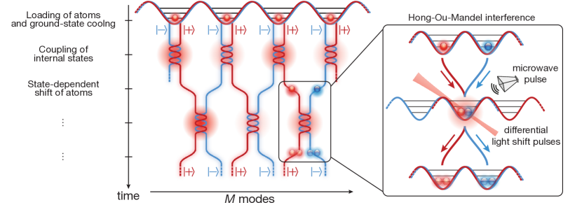
In this article, we propose to use ultracold atoms in state-dependent optical lattices as a scalable architecture for boson sampling with hundreds of bosons. We also report on the experimental realization of the basic building block of the proposed boson-sampling machine, demonstrating the Hong-Ou-Mandel interference between two atoms trapped in state-dependent optical lattices. In our scheme, atoms cooled into their motional ground state play the role of identical bosons, while the lattice site as well as two internal atomic states serve as the bosonic modes. Distant modes, associated with different lattice sites, are brought together by state-dependent shift operations, which are realized with polarization-synthesized optical lattices [87, 88]. Modes that are spatially overlapped are coupled in pairs, by a combination of microwave and site-resolved optical pulses, realizing the analog of phase-programmable photonic quantum circuits [89, 90].
It should be mentioned that based on a similar motivation to establish a quantum advantage, other NISQ proposals alternative to photonic boson samplers have been put forward in the past years relying on trapped ions [91, 92, 93], superconducting circuits [94], and neutral atoms with microwave assisted tunneling [95].
II Boson sampling with atoms in optical lattices
A boson sampling quantum machine is in essence an -port quantum circuit traversed simultaneously by identical bosons that do not interact with each other. As there are no interactions between the particles, such a quantum circuit behaves as a linear interferometer, mapping each input mode into a superposition of the output modes,
| (1) |
Here, is the operator creating a boson in the -th mode, and is the matrix element of a unitary transformation , which is randomly chosen from the uniform distribution (i.e., Haar measure) over all unitaries. The randomness of ensures that no particular feature can be exploited to efficiently simulate the boson sampler machine with a classical computer.
By detecting the occupation of the output modes, the machine thus directly samples from the probability distribution . Here, denotes the number of bosons in the -th output mode, and represents the initial state with identical bosons, each occupying a particular input mode. According to best-known algorithms [72], sampling from cannot be performed efficiently with classical computers, as it is bound to computing the permanent of matrices, which requires a computation time of order [96].
Importantly, to be hard to simulate by a classical computer, a boson sampler must have a number of modes much larger than that of particles, [50]. The gold standard satisfying this condition is given by the scaling law because it ensures that detecting two or more particles in any of the output modes has a small probability [97]. In fact, only when the output modes are singly occupied, i.e., for the so-called collision-free outcomes, does the conjectured hardness of boson sampling hold [50]. We therefore assume such a quadratic scaling in this paper. It should, however, be emphasized that this scaling has so far only been experimentally realized with a relatively small number of particles, , by photonics devices [71].
In the remainder of this section, we develop a concept how to implement such a boson sampling quantum machine with ultracold atoms in state-dependent optical lattices. We start with the key idea of how to construct arbitrary quantum circuits, and then discuss initialization and detection.
II.1 Arbitrary quantum circuits using polarization-synthesized optical lattices
Figure 1 illustrates how to “wire” an arbitrary quantum circuit using ultracold atoms in state-dependent optical lattices. The idea here is to use the lattice sites along with two internal states of the atom, and , to represent the modes of the quantum circuit, so that lattice sites accommodate modes. Modes associated with adjacent sites are connected in pairs by state-dependent shift operations.
Such state-dependent shift operations can be performed using polarization-synthesized optical lattices [87]. This piece of technology rely on the synthesis of polarization states of light to create two movable, fully independent periodic potentials,
| (2) |
which selectively trap atoms in either the or internal state. Here, represents the trap depth and the position of the respective periodic potentials, is the coordinate along the lattice direction, and the wavelength of the lattice laser. The underlying concept of state-dependent optical potentials is suited to atomic species such as Rb and Cs [98, 99]. In this work, we will consider specifically the case of 133Cs, where the internal modes are the hyperfine states and , and is set to the value of , for which the trapping potential of right and left circularly polarized light selectively trap the two internal states.
The lattice potentials must be chosen sufficiently deep, with being of order of a few hundred recoil energies, to prevent atoms from tunneling to the neighboring sites. In such a deep-lattice regime, one can shift the atoms to the adjacent sites in a state dependent manner by simply varying the relative position, , as a function of time . We have experimentally demonstrated [100] that repeated state-dependent shift operations preserve the coherence between the two internal states. Furthermore, we have shown in a recent work [101] that shifting the atoms by one lattice site can be rapid, with the minimum duration being bounded by the trap period at around .
Crucially, a quantum circuit such as the one in Fig. 1, where the modes are locally coupled in alternating pairs, allow one to realize any arbitrary unitary transformation of the input into the output modes [102, 103]. For a generic matrix , a minimum number of local operations is required, arranged in a circuit of -step depth [103]. Such an operation defines the basic unit of the quantum circuit, coupling together the modes associated with a given lattice site,
| (3) |
where and are parameters depending on the particular site and time step. A programmable quantum device of this kind is said to be completely controllable [104].
We propose to implement through composite pulses, where two types of elementary operations are stacked together: local phase imprints and global Hadamard pulses . In fact, for any , one can find suitable angles and yielding the following decomposition:
| (4) |
where imprints onto the two modes a relative phase depending on the lattice site, whereas acts on all sites identically, realizing the equivalent of a beam splitter (here, represent the Pauli matrices). Note that the local common-mode phase shift by , which appears in Eq. (4), can be avoided by conveniently adapting the algorithm by Clements et al. [103] to use instead of as the basic unit.
The decomposition of in Eq. (4) reveals a direct analogy to phase-programmable photonic circuits [89, 90]. Their structure reveals however an important difference: for ultracold atoms, a single spatial dimension suffices to wire the circuital modes, whereas at least two dimensions are necessary for photonic devices [70]. The advantage of ultracold atoms simply arises from the fact that massive particles can be held in a specific location by a trapping potential.
The global Hadamard gates are readily implemented by means of microwave pulses, which act homogeneously on all lattice sites and require a time of order of . The local operator can be realized by exploiting the differential Stark shift that is produced by an array of laser beams focused on the target lattice sites through a high-numerical-aperture objective lens [105, 106, 107]. Exploiting the vector polarizability of alkali atoms [98], one can imprint a purely differential phase shift onto the atoms by means of a circularly polarized light field. For Cs atoms, this condition is fulfilled when the wavelength of the addressing light field is chosen at . Such local pulses also require that the addressing beam has a nonzero component along the quantization axis. This additional condition can be met by tilting the quantization axis with respect to the lattice direction (see Appendix A).
The differential phase shift is directly controlled by the product of the laser intensity and pulse duration. We estimate that the addressing pulses can be realized in about using approximately of laser power per addressed lattice site. These pulses have a small impact on the coherence time of the atoms, because the probability that an atom scatters a photon off the addressing beam is approximately .
It is worth noting that the composite pulse scheme proposed to implement offers an important advantage over other schemes that use local resonant pulses to couple the two hyperfine states, . The reason for this is the difference in sensitivity to the crosstalk caused by the light field at the sites adjacent to the target lattice site. Differential Stark shift pulses, as in the proposed scheme, depend on the intensity of the addressing laser beams in their Hamiltonian, while resonant pulses directly depend on the respective electric fields. This different sensitivity implies that for the same intensity leaking to the neighboring sites, crosstalk errors are smaller in the proposed scheme: the crosstalk infidelity is proportional to in the proposed scheme, in contrast to in the resonant pulse schemes.
II.2 Initializing an array of identical atoms
Atom sorting techniques have recently been demonstrated [108, 109, 110, 88, 111, 112], where movable optical potentials are used to deterministically fill a predefined array of optical traps with one atom each. At present, the record in the number of resorted atoms is at around , and ideas exist how to boost this number up to 1000 by parallel resorting the atoms with a two-dimensional state-dependent optical lattice [88]. Once loaded into the desired sites of an optical lattice, atoms can be cooled to their motional ground state using sideband cooling techniques, making them indistinguishable in their mechanical degrees of freedom. Ground state probabilities above have already been achieved for atoms trapped in optical tweezers [113, 111, 114, 115], whereas higher values above are expected [116] for more tightly confined atoms in a three-dimensional optical lattice.
II.3 Detection of individual atoms
The final state is measured by recording a fluorescence image of the atoms [117, 107]. Using a high-resolution objective lens, the positions of the individual atoms in the optical lattices can be reconstructed with a high fidelity, exceeding . Standard fluorescence-imaging techniques, however, only give information about the occupation of modes belonging to distinct lattice sites. To also resolve the occupation of modes associated with the same site, a state-sensitive detection scheme resolving the two hyperfine states, , is needed. For this purpose, a long-distance state-dependent transport operation can be used to realize an optical Stern-Gerlach detection, mapping the two internal states to different lattice sites [118, 119]. Alternatively, one can use a magnetic Stern-Gerlach detection scheme in a multilayer optical lattice [120].
A particle number resolving detection is more demanding. Standard fluorescence imaging is not suitable because of light-induced collisions, which only allow the parity of the occupation number to be measured [121]. One approach is to distribute the atoms to multiple sites prior to fluorescence imaging [122], similar to spatial multiplexing in photonic devices [63]. An improved version of this approach consists in using a pinning lattice to detect the atoms [123, 124]. Alternatively, one can exploit interaction blockade to induce occupation-dependent tunneling to distinct sites of an optical lattice [120].
III Scaling law of an atom-boson-sampling machine
To appreciate the quantum advantage of an atom boson sampler over classical machines, we study in this section the sampling rate, , as a function of the number of bosons.
III.1 Ideal boson sampler
In the ideal case of no atom losses, the sampling rate is simply given by the repetition rate at which bosons are made to interfere with each other in a quantum circuit of modes. Three terms determines this rate,
| (5) |
where is the time for executing the quantum circuit, is the time for preparing the initial state of atoms, and is the time for detecting the atoms in the output modes.
To estimate the execution time , we assume that local Stark shift pulses can be carried out in parallel by optically addressing all sites simultaneously [16, 125]. The time for executing the quantum circuit is thus proportional to the total number of steps, which in turn is equal to the number of modes (see Sec. II.1). Considering that the number of modes is given by , as previously reasoned, we find that the execution time has a quadratic dependence on the number of bosons, , where is the time to perform the single step.
The initialization time is proportional to for linear atom sorting [109, 108], and to for parallel atom sorting [88]. For simplicity, we assume that this time is fixed at , since the initialization of atoms can be efficiently performed in less than this time [27]. Likewise, we consider the detection time to be fixed, , since both positions and spin can be efficiently detected for all atoms in a single operation relying on fluorescence imaging [118, 119].
Furthermore, if we post-select only those events with all atoms populating a different output mode (i.e., the so-called collision-free events), because these are the events hard to simulate with a classical machine, the sampling rate is reduced by a constant factor in the limiting case of large [97], leading to .
Thus, we conclude that under ideal conditions, an atom boson sampler can draw events from the boson distribution efficiently, since its computation time scales with for sufficiently large (i.e., polynomial time complexity). In contrast, classical computer simulations require an exponentially longer time to perform the same task, which scales with [72], as mentioned earlier.
 [59],
[59],
 [60], and
  [61],
while the best reported boson sampling experiment with
[61],
while the best reported boson sampling experiment with  [71].
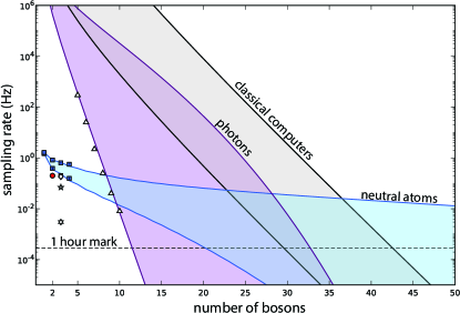
Our proof-of-principle experiment, described in Sec. IV, is marked with
[71].
Our proof-of-principle experiment, described in Sec. IV, is marked with  symbol.
The numerical results obtained with the master equation approach (see Appendix D) are indicated with
symbol.
The numerical results obtained with the master equation approach (see Appendix D) are indicated with  symbols, with the vertical bars indicating the 1- statistical uncertainty.
III.2 NISQ boson sampler
In a realistic scenario typical of NISQ devices, the sampling rate is significantly degraded by state preparation errors, atom losses while executing the quantum circuit, and detection inefficiency. Along the lines of Refs. [68, 72], we estimate the sampling rate as:
| (6) |
where is the detection efficiency, the cooling efficiency into the motional ground state, and is the probability that all atoms survive. We indeed consider the sampling problem where no particle is lost for the reasons outlined in Sec. I.
Equation (6) immediately reveals that the computation time scales exponentially with the number of particles. It is therefore important to carefully evaluate the expression in Eq. (6) to determine the conditions when an atom boson sampler offers a quantum advantage over classical computer simulations.
As described in Sec. II, cooling and detection of ultracold atoms can be done efficiently, with reported values of and above [113, 111, 114, 115] and [118], respectively. The survival probability in Eq. (6) depends on two main loss mechanisms, which we discuss below.
The first mechanism responsible for the loss of atoms is represented by collisions of one of the trapped atoms with a molecule from the background gas at room temperature, causing the atom to be ejected from the trap. For atoms, the probability that no collision with the background gas occurs during a single step is given by the exponential formula , where is the background-gas-limited mean lifetime of a single atom.
The second mechanism leading to the loss of atoms is given by inelastic collisions of atoms occupying the same lattice site. Inelastic collisions cause the atoms to change their hyperfine state [126, 127, 128], and to acquire kinetic energy, thus leaving the motional ground state where they are initially prepared. Such inelastic collisions typically result in the loss of atoms from the trap because of the large energy separation between hyperfine states (several between adjacent states, between different states, expressed in frequency units). Three-body collisions are neglected because the probability of trios (and even higher occupations) compared to that of pairs is negligible in the limit of large (see Appendix B). To account for the two-atom lossy collisions, we introduce the survival probability of a pair of atoms located in the same lattice site, given by , where is the mean lifetime limited by two-body collisions. Note that for simplicity we use the same constant without differentiating between the three possible spin configurations of the two bosons occupying the same site. To estimate the number of pairs of atoms that can collide onsite, we make the conservative assumption that all states of bosons have equal probability of being occupied at every time step. Thereby, we overestimate the probability of inelastic collisions at the initial steps since the atoms are first prepared in different sites. Under the above assumption of uniform distribution and in the limiting case of large , the probability of finding sites occupied by exactly a pair of atoms can be estimated as (Appendix B). For example, refers to the case where all atoms occupy distinct lattice sites (collisionless subspace). The overall survival probability per time step, limited by two-body lossy collisions, can thus be obtained by the evaluating the following sum,
| (7) |
where the expression on the right-hand side holds in the limit of large (Appendix B). For weak two-body losses, , the survival probability decays as , while in the limiting case of strong losses the survival probability approaches , i.e., the probability of the collisionless subspace.
Combining the two loss mechanisms, the survival probability per step is simply given by . Because the execution of the quantum circuit requires steps, the total survival probability of atoms is thus
| (8) | ||||
A comparison of the two terms in Eq. (8) shows that under typical conditions two-body collisions are the dominant loss mechanism for . As will be argued below, realistic experiments are expected to operate with a number of atoms below this threshold.
To evaluate in Eq. (6), we consider two different scenarios, which are based on conservative and state-of-the-art assumptions, respectively. In the conservative scenario, we assume a step duration and a mean lifetime limited by two-body collisions , while in the state-of-the-art scenario, we consider and . For the initialization and detection times, we assume and , with efficiencies of and for the conservative scenario, and for the state-of-the-art scenario. For the mean lifetime limited by background gas collisions, we take in both scenarios. The threshold value is larger than atoms in both scenarios, implying that for a realistic number of atoms the dominant loss mechanism is inelastic two-body collisions rather than collisions with the background gas.
In Fig. 2, we show the sampling rate as a function of the number of particles , computed for an atom boson sampler with conservative and state-of-the-art assumptions (blue curves). To identify the regime of quantum advantage, we present in the same figure the sampling rate of best algorithms [72] simulating a boson sampler using a standard laptop and the Tianhe-2 supercomputer (gray curves). For the sake of comparison, we also report in the figure the sampling rate expected for NISQ photonic devices (purple curves) for a conservative and state-of-the-art scenario; see Appendix C details.
IV Experimental demonstration of the Hong-Ou-Mandel interference
We have performed a proof-of-principle experiment with two atoms in a four-mode interferometer, which demonstrates the Hong-Ou-Mandel effect with atoms, as schematically shown in the inset of Fig. 1. Such an experiment establishes the basic building block of the envisaged boson sampling machine.
The Hong-Ou-Mandel effect with atoms has been previously demonstrated experimentally using movable optical tweezers [129], an optical lattice superimposed to a box potential [130], and a free-fall atom interferometer [101]. Compared to these setups [131] and to related proposals based on microwave-induced tunneling [95], our setup is distinguished by the way modes are coupled, where the the atoms are moved with state-dependent shift operations [87] instead of having them tunnel through an optical potential barrier. Our approach enables faster operations on the scale of few microseconds instead of milliseconds.
The setup used for our experimental demonstration is schematically depicted in Fig. 3(a). We start with a handful of Cs atoms, which are sparsely loaded in a one-dimensional polarization-synthesized optical lattice [87]. Using the atom sorting technique presented in Ref. [88], a pair of atoms is then selected and repositioned to a relative distance of twenty lattice sites with a success rate of about , mainly limited by an incorrect detection of the initial distance between the two atoms [117].
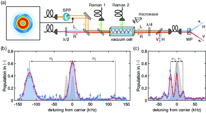
To make the two atoms identical, we cool them to the ground state of the lattice site potential in which they are respectively trapped. For this purpose, we use resolved sideband cooling, where the sideband transitions are driven by microwave radiation [132] for the direction along the lattice axis and by two Raman lasers [113] for the transverse directions. The optical lattice provides a tight confinement ( sideband) along its longitudinal direction, while a hollow-tube potential collinear with the lattice axis also provides a tight confinement ( sideband) in the transverse directions. These trap frequencies are much larger than the recoil frequency (), thus ensuring that the Lamb-Dicke condition necessary for ground state cooling is fulfilled. We alternate between microwave and Raman sideband cooling 3 times in order to cool the atoms in both the longitudinal and transverse directions. By allowing a slight ellipticity of the transverse potential, we lift the degeneracy of the transverse motional states, allowing Raman sideband cooling to be effective along both transverse directions. At the end of the cooling process, the atoms are polarized in the state with a probability of .
Figures 3(b) and 3(c) report a typical microwave and Raman sideband spectrum recorded after the cooling procedure, demonstrating a pronounced suppression of the cooling (blue detuned) sideband with respect to the heating (red detuned) sideband. From the ratio of the sideband amplitudes [133], we derive a ground state probability of for the longitudinal direction and of for each transverse direction. Thus, the overall probability of occupying the motional ground state can be estimated as .
After sideband cooling, a magnetic field gradient along the lattice direction () is ramped up in and maintained until before detecting the atoms by fluorescence imaging. The magnetic field gradient induces a position-dependent Zeeman shift ( per lattice site), which is used to selectively transfer one of the two atoms to the state. We perform such a selective spin flip by addressing the target atom with a microwave narrow-bandwidth pulse (Gaussian shape, rms width). Spin-flip errors are clearly visible in the final fluorescence image, allowing them to be removed by post-selection. The atom thus selected is then adiabatically transported in to the site of the second atom by shifting the lattice potential. With the two atoms occupying the same site, we apply a fast microwave pulse (square shape, duration). This pulse acts much like the beam splitter of a Hong-Ou-Mandel optical interferometer, erasing the which-way information of the two impinging particles. Last, we shift the lattice potential to map the the internal states, and , to two different locations 10 lattice sites apart, where the atoms are detected by position-resolved fluorescence imaging.
Two identical atoms are expected to bunch together in the same lattice site with unit probability because of the Hong-Ou-Mandel interference (quantum statistics). In practice, however, the two atoms can differ from each other because of their motional states. For two atoms in orthogonal states (i.e., fully distinguishable particles), the outcomes resemble those obtained from the toss of two independent coins, yielding a bunching probability of (classical statistics). For partially distinguishable atoms like ours, the probability to bunch is determined by the so-called quantum purity of the state, , which represents the probability of the two atoms to be indistinguishable: . Thus, the Hong-Ou-Mandel interference is established if we can show that the bunching probability of the two atoms fulfills .
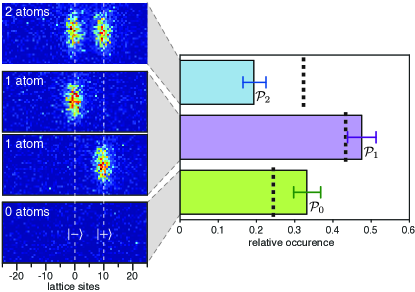
In the experiment, we distinguish three outcomes corresponding to the detection of zero, one, and two atoms in the final fluorescence image. Figure 4 shows the experimentally recorded probability for each of them. When both atoms are positively detected, the atoms are found at different locations, 10 sites apart (see fluorescence image in Fig. 4). Importantly, such an outcome can only occur when the two atoms have not bunched together. Its probability is thus directly related to through the expression: , where is the single-atom survival probability. From the measurement of and , we therefore obtain , which exhibits a 5- deviation from the reference value .
Such a value of establishes that the Hong-Ou-Mandel interference of the two atoms occurs with a probability . We expect that can be significantly improved in the future with more efficient ground-state cooling of the atoms in a three-dimensional optical lattice. An analysis of all experimental outcomes, including those with zero and one atom detected, yields a value of that is statistically consistent with the value we have derived from only (see Appendix E).
V Conclusions
In this work, we have presented a scheme for the realization of programmable NISQ circuits with neutral atoms in state-dependent optical lattices. Quantum circuits based on the proposed scheme can be easily reprogrammed and scaled up to hundreds of modes. Both repogrammability and scalability are key to realize large random unitaries a prerequisite for any large-scale boson sampling machine. Furthermore, we have experimentally demonstrated the basic building block of an atom Boson sampling machine by executing a quantum circuit with four modes and two indistinguishable atoms. We observed the atoms bunching in pairs, thus revealing their bosonic nature. The Hong-Ou-Mandel interference signal of the atom bunching is found to deviate from the outcome predicted for distinguishable (i.e., classical) particles by 5 . The degree of indistinguishability of the atoms is determined by the probability of occupying the motional ground state in the potential well of an optical lattice site. We independently measured the motional ground state occupancy of the atoms and showed that it is in good agreement with the ground state occupancy inferred from the observed bunching probability.
We have discussed in detail how to wire quantum circuits using a one-dimensional state-dependent optical lattice. Our analysis of NISQ devices has shown that controlling more than lattice sites will be required to reach a quantum advantage over best supercomputers. Controlling such a large number of lattice sites may become difficult to realize in a one-dimensional geometry. However, our scheme can be readily extended to two-dimensional state-dependent optical lattices [134], leading to a more compact and less resource-intensive platform.
For future studies, it will be interesting to investigate the role of controlled coherent collisions among atoms [135], which can be exploited to imprint collisional phases onto the quantum state when two or more particles meet at the same site [136]. The inclusion of such nonlinearities is shown to augment the amount of correlations in the output distribution [137]. For this reason, there is a potential that simulating a nonlinear boson sampler with classical computers will be an even harder task than the original linear problem.
Appendix A Quantization axis tilt
Since the addressing beam is tightly focused onto several sites of the optical lattice, its direction must be perpendicular to the optical lattice itself. With this geometrical constraint, the only way to fulfill the condition stated in Sec. II.1, namely that the quantization axis must have a nonzero component along the addressing beam, is to allow the quantization axis to form an angle, , with respect to the optical-lattice direction.
However, a tilt of the quantization axis by with respect to the optical lattice causes an additional, undesired effect. A wobble of the optical lattice potential’s depth, , is produced during state-dependent shift operations, with its magnitude being an increasing function of . For small angles, though, the extent of this effect is very small. For example, for , it only causes a reduction of the lattice depth by during atom transport, which can be easily taken into account and compensated for by designing the transport operations.
Appendix B Pair distribution and extended model
In the limit of large and after averaging over random quantum circuits, the state of the bosons is described by a uniform statistical mixture [97]. When large, the density matrix can be written as , where is the probability of finding sites populated by exactly a pair of atoms, and represents a normalized uniform sum of all states matching this criteria. Notice that here we ignore all states where at least a site is occupied by more than two atoms. Although valid for large , this approximation is not justified for intermediate values of . Thus, in the following we derive a general expression to account for the probability of finding sites occupied by exactly a pair of particles, and sites occupied by a particle trio. To calculate we start by determining the number of configurations containing sites occupied by exactly a trio of atoms. For that, we should first consider that there are different ways in which trios can be arranged in sites (for simplicity, we consider to be even). Since each site has triple occupation, there are four possible spin configurations, , , and , and the previous number of combinations should be multiplied by to obtain the total number of configurations. Next, we should consider that there are combinations in which pairs can be arranged in the remaining sites. This number, should be multiplied by to account for the three different spin configurations , , and . Now, there are different configurations in which the remaining particles can be placed in sites. Since in this case each site is singly occupied, there are only two possible spin configurations, and . Finally, all this should be divided by the overall number of possible bosonic configurations, which is given by the multiset coefficient . The probability of having sites occupied by pairs and sites occupied by trios is then given by
| (9) | |||||
As anticipated in the main text, in the limit of large Eq. (9) converges to a Poissonian distribution
| (10) |
with average value . Here, the constant factor denotes the ratio , which in the main text has been simply assumed equal to 1.
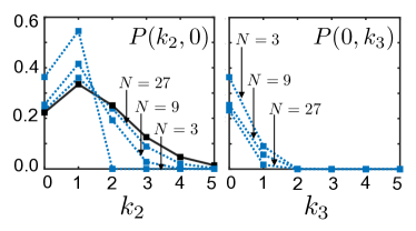
In Eq. (10) we see that, for large , the probability of having a particle trio vanishes, and the probability associated to the collision-free subspace (the subspace of states where all atoms are at different sites), i.e. , tends to . The situation for intermediate values of has been illustrated in Fig. 5, where (on the left) and (on the right) have been plotted for and and for . In the left figure, one can see how Eq. (9) (blue dotted curves) tends to Eq. (10) (black solid curve) when increasing . In the right figure, we see that has a non-negligible value (between and ) for or .
Now, let us consider how the uniform state evolves according to two-body losses. Assuming that the survival probability of a state with sites occupied by a particle pair decays as , we get that, for large , the total survival probability will be given by . This sum can be rewritten as
| (11) |
which is equivalent to Eq. (7) in the main text. Taking into account particle trios, the total survival probability is
| (12) |
instead. Note that a particle trio decays three times faster than a particle pair. This can be understood through the action of (defined in appendix D) in a state with sites containing a particle trio, that is, , when ignoring single-particle loss.
In Fig. 2 and in Appendix D, this model is used instead of Eq. (7), as it is more accurate to describe the scenario for small number of particles. Equation (9) can be further extended to account for the cases with quartets, quintets, etc. These have not been considered as their contribution is negligible even from small number of particles.
Appendix C Scaling law for photonic and classical boson samplers
For a photonic boson sampler, the sampling rate is given by
| (13) |
where is the rate in which indistinguishable photons are created and is the success probability of a single photon to complete the boson sampling experiment from state preparation, to circuit transmission, to single photon detection. The success probability is a product of a fixed probability , that does not scale with the number of modes in the circuit (preparation and detection) and the circuit transmission probability , which accounts for the chance that a photon can be absorbed at each beamsplitter. In this manuscript we only consider square circuits with which implies that the transmission probability depends quadratically on the number of photons [103].
Our conservative values (lower edge of the blue area in Fig. 2) are based on Ref. [71]. The authors use a single-photon source working at MHz and report a boson sampling rate of Hz for 5-photons in a optical circuit. The transmission probability through the entire circuit is reported as and correspondingly , which in turn allows us to extract the fixed preparation and detection probability of . For the state-of-the-art estimate (upper edge of the blue area in Fig. 2) we assume an overall increased fixed preparation and detection probability of [69].
For a classical boson sampler, the time required by a recently developed algorithm Ref. [72] based on Metropolised independent sampling produce a valid sample scales as
| (14) |
where relates to the speed of the classical computer. This value has been reported to be s in the case of the Tianhe-2 supercomputer [96]. For the case of a regular computer we choose this value to be s.
Appendix D Benchmark with exact simulations
Here, we introduce the master equation model used to benchmark the sampling-rate formula for a small number of particles. In our model, an -particle initial state is given by where and . Here, is the number operator acting on mode . The evolution of such a quantum state is given by
| (15) |
where are the coherent operations at step , and represents particle decay acting for a time . Because our reduced Hilbert space accounts only for states in the -particle subspace, the final state is a pure state, and the survival probability of the process is then characterized by its modulus, . The Hermitian operator is
| (16) |
Here, is the number operator acting on lattice site , where , with being a Fock state representing atoms in site . In Eq. (16), the first and second terms represents single-body and two-body decay, respectively. Notice that acts as in states with zero pairs and as in states with sites populated by particle pairs.
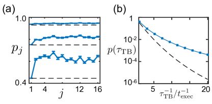
In the following we benchmark the simplified models used in the main text with exact numerical simulations for . For that, we evaluate the appropriateness of Eq. (12) as a lower bound for the survival probability at every time step. According to Eq. (15), the survival probability from time step to is given by , where .
In Fig. 6 (a), we plot versus and for different values of . For clarity, we omit the effect of single-particle losses as their effect is trivial. For , there is an almost exact correspondence between (black dashed line) and (blue solid curve) for all steps , suggesting that, for weak losses, Eq. (12) provides an accurate description of the decay of the success probability at every time step. Notice that, for simplicity, we chose a pure state with a uniform probability distribution as the initial state. For lower values of , such as or , this correspondence only holds for the initial state, while for the rest of the steps, . In Fig. 6 (b), we evaluate in function of (blue solid curve), and conclude that gives a correct description of two-body losses for and it is a valid lower bound for . Although this has been numerically shown for , to the best of our knowledge, there is no reason to believe in the change of this tendency for larger values of .
Appendix E Monte Carlo analysis of the Hong-Ou-Mandel experiment
In order to extract from the experimental results, it is important to consider that atoms bunched in the same site cannot be directly detected by fluorescence imaging without losing them. In fact, measurements performed in our apparatus on bunched atoms show that with a probability no atom is left, while with a probability just a single atom is detected in the final fluorescence image as a consequence of light-induced collisions [138]. Hence, identical atoms lead to the detection of either zero or one atom, while distinguishable atoms are both detected if after the pulse they occupy different internal states. Examples of the three possible outcomes with , and atoms detected are shown in Fig. 4(a).
To measure the single-atom survival probability we performed independent measurements similar to the HOM interference experiment outlined in the main text, omitting the microwave pulse. Without the microwave pulse =0 which enables a direct measurement of . From this experiment we determine . The value of is limited by losses at the beginning of the transverse cooling process, which could be avoided in the future with an improved experimental procedure.
We employ a Monte Carlo analysis to more rigorously analyze the measured statistical outcomes. Our Monte Carlo simulation mimics the experimental HOM interference sequence outlined in the main text. The Monte Carlo simulation uses the predetermined light-induced collision probability and the single-atom survival probability . Further input parameters are the indistinguishability of the two atoms, the addressing probability of the narrow bandwidth MW pulse, and the probability to successfully reconstruct the position of the atoms. We perform a nonlinear least-squares fit of the generated Monte Carlo events to the measured data to extract the underlying experimental parameters, yielding .
Acknowledgements.
We acknowledge financial support from the NRW-Nachwuchsforschergruppe “Quantenkontrolle auf der Nanoskala”, the Deutsche Forschungsgemeinschaft SFB project OSCAR, the Basque Government with PhD grant PRE-2015-1-0394, the Junta de Andalucía (grants P20-00617 and US-1380840), the Spanish Ministry of Science, Innovation, and Universities (grants PID2019-104002GB-C21 and PID2019-104002GB-C22), the National Natural Science Foundation of China (grant 12075145), and Science and Technology Commission of Shanghai Municipality (grant 2019SHZDZX01-ZX04). A. A acknowledges support from the Alexander von Humboldt Foundation, C. R. from the Studienstiftung des deutschen Volkes. C. R. and I. A. contributed equally to this work.References
- Blatt and Wineland [2008] R. Blatt and D. Wineland, “Entangled states of trapped atomic ions,” Nature 453, 1008 (2008).
- Ladd et al. [2010] T. D. Ladd, F. Jelezko, R. Laflamme, Y. Nakamura, C. Monroe, and J. L. O’Brien, “Quantum computers,” Nature 464, 45 (2010).
- Weiss and Saffman [2017] D. S. Weiss and M. Saffman, “Quantum computing with neutral atoms,” Phys. Today 70, 44 (2017).
- Monz et al. [2011] T. Monz, P. Schindler, J. T. Barreiro, M. Chwalla, D. Nigg, W. A. Coish, M. Harlander, W. Hänsel, M. Hennrich, and R. Blatt, “14-Qubit Entanglement: Creation and Coherence,” Phys. Rev. Lett. 106, 130506 (2011).
- Kaufman et al. [2015] A. M. Kaufman, B. J. Lester, M. Foss-Feig, M. L. Wall, A. M. Rey, and C. A. Regal, “Entangling two transportable neutral atoms via local spin exchange,” Nature 527, 208 (2015).
- Lekitsch et al. [2017] B. Lekitsch, S. Weidt, A. G. Fowler, K. Mølmer, S. J. Devitt, C. Wunderlich, and W. K. Hensinger, “Blueprint for a microwave trapped ion quantum computer.” Sci. Adv. 3, e1601540 (2017).
- Wang et al. [2016] Y. Wang, A. Kumar, T. Y. Wu, and D. S. Weiss, “Single-qubit gates based on targeted phase shifts in a 3D neutral atom array,” Science 352, 1562 (2016).
- Barredo et al. [2018] D. Barredo, V. Lienhard, S. de Léséleuc, T. Lahaye, and A. Browaeys, “Synthetic three-dimensional atomic structures assembled atom by atom,” Nature 561, 79 (2018).
- Zeng et al. [2017] Y. Zeng, P. Xu, X. He, Y. Liu, M. Liu, J. Wang, D. J. Papoular, G. V. Shlyapnikov, and M. Zhan, “Entangling Two Individual Atoms of Different Isotopes via Rydberg Blockade,” Phys. Rev. Lett. 119, 160502 (2017).
- Bernien et al. [2017] H. Bernien, S. Schwartz, A. Keesling, H. Levine, A. Omran, H. Pichler, S. Choi, A. S. Zibrov, M. Endres, M. Greiner, V. Vuletić, and M. D. Lukin, “Probing many-body dynamics on a 51-atom quantum simulator,” Nature 551, 579 (2017).
- Wang et al. [2017a] Y. Wang, M. Um, J. Zhang, S. An, M. Lyu, J.-N. Zhang, L.-M. Duan, D. Yum, and K. Kim, “Single-qubit quantum memory exceeding ten-minute coherence time,” Nature. Photon. 11, 646 (2017a).
- Bermudez et al. [2017] A. Bermudez, X. Xu, R. Nigmatullin, J. O’Gorman, V. Negnevitsky, P. Schindler, T. Monz, U. G. Poschinger, C. Hempel, J. Home, F. Schmidt-Kaler, M. Biercuk, R. Blatt, S. Benjamin, and M. Müller, “Assessing the Progress of Trapped-Ion Processors Towards Fault-Tolerant Quantum Computation,” Phys. Rev. X 7, 257 (2017).
- Zajac et al. [2017] D. M. Zajac, A. J. Sigillito, M. Russ, F. Borjans, J. M. Taylor, G. Burkard, and J. R. Petta, “Resonantly driven CNOT gate for electron spins,” Science 359, 439 (2017).
- Levine et al. [2019] H. Levine, A. Keesling, G. Semeghini, A. Omran, T. T. Wang, S. Ebadi, H. Bernien, M. Greiner, V. Vuletić, H. Pichler, and M. D. Lukin, “Parallel Implementation of High-Fidelity Multiqubit Gates with Neutral Atoms,” Phys. Rev. Lett. 123, 170503 (2019).
- Chen et al. [2021] Z. Chen et al., “Exponential suppression of bit or phase errors with cyclic error correction,” Nature 595, 383 (2021).
- Pogorelov et al. [2021] I. Pogorelov, T. Feldker, C. D. Marciniak, L. Postler, G. Jacob, O. Krieglsteiner, V. Podlesnic, M. Meth, V. Negnevitsky, M. Stadler, B. Höfer, C. Wächter, K. Lakhmanskiy, R. Blatt, P. Schindler, and T. Monz, “Compact Ion-Trap Quantum Computing Demonstrator,” PRX Quantum 2, 020343 (2021).
- Wilczek [2016] F. Wilczek, “Physics in 100 years,” Phys. Today 69, 32 (2016).
- Das and Chakrabarti [2008] A. Das and B. K. Chakrabarti, “Colloquium: Quantum annealing and analog quantum computation,” Rev. Mod. Phys. 80, 1061 (2008).
- Cirac and Zoller [2012] J. I. Cirac and P. Zoller, “Goals and opportunities in quantum simulation,” Nature Phys. 8, 264 (2012).
- Bloch et al. [2012] I. Bloch, J. Dalibard, and S. Nascimbène, “Quantum simulations with ultracold quantum gases,” Nature Phys. 8, 267 (2012).
- Blatt and Roos [2012] R. Blatt and C. F. Roos, “Quantum simulations with trapped ions,” Nature Phys. 8, 277 (2012).
- Aspuru-Guzik and Walther [2012] A. Aspuru-Guzik and P. Walther, “Photonic quantum simulators,” Nature Phys. 8, 285 (2012).
- Houck et al. [2012] A. A. Houck, H. E. Türeci, and J. Koch, “On-chip quantum simulation with superconducting circuits,” Nature Phys. 8, 292 (2012).
- van Houcke et al. [2012] K. van Houcke, F. Werner, E. Kozik, N. Prokof’ev, B. Svistunov, M. J. H. Ku, A. T. Sommer, L. W. Cheuk, A. Schirotzek, and M. W. Zwierlein, “Feynman diagrams versus Fermi-gas Feynman emulator,” Nat. Phys. 8, 366 (2012).
- Georgescu et al. [2014] I. M. Georgescu, S. Ashhab, and F. Nori, “Quantum simulation,” Rev. Mod. Phys. 86, 153 (2014).
- Gross and Bloch [2017] C. Gross and I. Bloch, “Quantum simulations with ultracold atoms in optical lattices,” Science 357, 995 (2017).
- Ebadi et al. [2021] S. Ebadi, T. T. Wang, H. Levine, A. Keesling, G. Semeghini, A. Omran, D. Bluvstein, R. Samajdar, H. Pichler, W. W. Ho, S. Choi, S. Sachdev, M. Greiner, V. Vuletić, and M. D. Lukin, “Quantum phases of matter on a 256-atom programmable quantum simulator,” Nature 595, 227 (2021).
- Biamonte et al. [2017] J. Biamonte, P. Wittek, N. Pancotti, P. Rebentrost, N. Wiebe, and S. Lloyd, “Quantum machine learning,” Nature 549, 195 (2017).
- Benedetti et al. [2019] M. Benedetti, E. Lloyd, S. Sack, and M. Fiorentini, “Parameterized quantum circuits as machine learning models,” Quantum. Sci. Technol. 4, 043001 (2019).
- Parra-Rodriguez et al. [2020] A. Parra-Rodriguez, P. Lougovski, L. Lamata, E. Solano, and M. Sanz, “Digital-analog quantum computation,” Phys. Rev. A 101, 022305 (2020).
- Lund et al. [2017] A. P. Lund, M. J. Bremner, and T. C. Ralph, “Quantum sampling problems, BosonSampling and quantum supremacy,” npj Quantum Inf. 3, 15 (2017).
- Aaronson and Chen [2016] S. Aaronson and L. Chen, “Complexity-Theoretic Foundations of Quantum Supremacy Experiments,” arXiv (2016), arXiv:1612.05903 .
- [33] Gottesman–Knill theorem: D. Gottesman, “The Heisenberg Representation of Quantum Computers,” in Group22: Proceedings of the XXII International Colloquium on Group Theoretical Methods in Physics, edited by S. P. Corney, R. Delbourgo, and P. D. Jarvis (International Press, Cambridge, MA, 1999), pp. 32–43.
- Valiant [2002] L. G. Valiant, “Quantum Circuits That Can Be Simulated Classically in Polynomial Time,” SIAM. J. Comput. 31, 1229 (2002).
- Pednault et al. [2017] E. Pednault, J. A. Gunnels, G. Nannicini, L. Horesh, T. Magerlein, E. Solomonik, and R. Wisnieff, “Pareto-Efficient Quantum Circuit Simulation Using Tensor Contraction Deferral,” arXiv (2017), arXiv:1710.05867 .
- Dalzell et al. [2020] A. M. Dalzell, A. W. Harrow, D. E. Koh, and R. L. La Placa, “How many qubits are needed for quantum computational supremacy?” Quantum 4, 264 (2020).
- Preskill [2013] J. Preskill, “Quantum Entanglement and Quantum Computing,” in Proceedings of the 25th Solvay Conference on Physics: The theory of the quantum world, edited by D. Gross, M. Henneaux, and A. Sevrin (World Scientific, Singapore, 2013) p. 63.
- Harrow and Montanaro [2017] A. W. Harrow and A. Montanaro, “Quantum computational supremacy,” Nature 549, 203 (2017).
- Bouland et al. [2018] A. Bouland, B. Fefferman, C. Nirkhe, and U. Vazirani, “On the complexity and verification of quantum random circuit sampling,” Nat. Phys. 15, 159 (2018).
- Dalzell et al. [2021] A. M. Dalzell, N. Hunter-Jones, and F. G. S. L. Brandão, “Random quantum circuits transform local noise into global white noise,” arXiv (2021), arXiv:2111.14907 .
- Terhal and Divincenzo [2004] B. M. Terhal and D. P. Divincenzo, “Adaptive Quantum Computation, Constant Depth Quantum Circuits and Arthur-Merlin Games,” Quantum Inf. Comput. 4, 134 (2004).
- Bermejo-Vega et al. [2018] J. Bermejo-Vega, D. Hangleiter, M. Schwarz, R. Raussendorf, and J. Eisert, “Architectures for Quantum Simulation Showing a Quantum Speedup,” Phys. Rev. X 8, 021010 (2018).
- Bravyi et al. [2018] S. Bravyi, D. Gosset, and R. König, “Quantum advantage with shallow circuits,” Science 362, 308 (2018).
- Shepherd and Bremner [2009] D. Shepherd and M. J. Bremner, “Temporally unstructured quantum computation,” in Proceedings of the Royal Society A: Mathematical (2009) p. 1413.
- Bremner et al. [2016] M. J. Bremner, A. Montanaro, and D. J. Shepherd, “Average-Case Complexity Versus Approximate Simulation of Commuting Quantum Computations,” Phys. Rev. Lett. 117, 080501 (2016).
- Boixo et al. [2018] S. Boixo, S. V. Isakov, V. N. Smelyanskiy, R. Babbush, N. Ding, Z. Jiang, M. J. Bremner, J. M. Martinis, and H. Neven, “Characterizing quantum supremacy in near-term devices,” Nat. Phys. 14, 595 (2018).
- Neill et al. [2018] C. Neill et al., “A blueprint for demonstrating quantum supremacy with superconducting qubits,” Science 360, 195 (2018).
- Arute et al. [2019] F. Arute et al., “Quantum supremacy using a programmable superconducting processor,” Nature 574, 505 (2019).
- Wu et al. [2021] Y. Wu, W.-S. Bao, S. Cao, F. Chen, M.-C. Chen, X. Chen, T.-H. Chung, H. Deng, Y. Du, D. Fan, M. Gong, C. Guo, C. Guo, S. Guo, L. Han, L. Hong, H.-L. Huang, Y.-H. Huo, L. Li, N. Li, S. Li, Y. Li, F. Liang, C. Lin, J. Lin, H. Qian, D. Qiao, H. Rong, H. Su, L. Sun, L. Wang, S. Wang, D. Wu, Y. Xu, K. Yan, W. Yang, Y. Yang, Y. Ye, J. Yin, C. Ying, J. Yu, C. Zha, C. Zhang, H. Zhang, K. Zhang, Y. Zhang, H. Zhao, Y. Zhao, L. Zhou, Q. Zhu, C.-Y. Lu, C.-Z. Peng, X. Zhu, and J.-W. Pan, “Strong Quantum Computational Advantage Using a Superconducting Quantum Processor,” Phys. Rev. Lett. 127, 180501 (2021).
- Aaronson and Arkhipov [2011] S. Aaronson and A. Arkhipov, “The computational complexity of linear optics,” in STOC ’11 Proceedings (ACM Press, New York, USA, 2011) p. 333.
- Gard et al. [2015] B. T. Gard, K. R. Motes, J. P. Olson, P. P. Rohde, and J. P. Dowling, “An Introduction to Boson-Sampling,” in From Atomic to Mesoscale (World Scientific, Singapore, 2015) p. 167.
- Scheel [2004] S. Scheel, “Permanents in linear optical networks,” arXiv (2004), arXiv:quant-ph/0406127 .
- Lim and Beige [2005] Y. L. Lim and A. Beige, “Generalized Hong Ou Mandel experiments with bosons and fermions,” New J. Phys. 7, 155 (2005).
- Glynn [2010] D. G. Glynn, “The permanent of a square matrix,” European Journal of Combinatorics 31, 1887 (2010).
- Aaronson [2011] S. Aaronson, “A linear-optical proof that the permanent is #P-hard,” Proceedings of the Royal Society A: Mathematical, Physical and Engineering Sciences 467, 3393 (2011).
- Valiant [1979] L. G. Valiant, “The complexity of computing the permanent,” Theoretical Computer Science 8, 189 (1979).
- Aaronson and Arkhipov [2013] S. Aaronson and A. Arkhipov, “BosonSampling Is Far From Uniform,” arXiv (2013), arXiv:1309.7460 .
- Gard et al. [2014] B. T. Gard, J. P. Olson, R. M. Cross, M. B. Kim, H. Lee, and J. P. Dowling, “Inefficiency of classically simulating linear optical quantum computing with Fock-state inputs,” Phys. Rev. A 89, 022328 (2014).
- Broome et al. [2013] M. A. Broome, A. Fedrizzi, S. Rahimi-Keshari, J. Dove, S. Aaronson, T. C. Ralph, and A. G. White, “Photonic boson sampling in a tunable circuit.” Science 339, 794 (2013).
- Tillmann et al. [2013] M. Tillmann, B. Dakić, R. Heilmann, S. Nolte, A. Szameit, and P. Walther, “Experimental boson sampling,” Nature Photon. 7, 540 (2013).
- Spring et al. [2013] J. B. Spring, B. J. Metcalf, P. C. Humphreys, W. S. Kolthammer, X.-M. Jin, M. Barbieri, A. Datta, N. Thomas-Peter, N. K. Langford, D. Kundys, J. C. Gates, B. J. Smith, P. G. R. Smith, and I. A. Walmsley, “Boson Sampling on a Photonic Chip,” Science 339, 798 (2013).
- Crespi et al. [2013] A. Crespi, R. Osellame, R. Ramponi, D. J. Brod, E. F. Galvão, N. Spagnolo, C. Vitelli, E. Maiorino, P. Mataloni, and F. Sciarrino, “Integrated multimode interferometers with arbitrary designs for photonic boson sampling,” Nature Photon. 7, 545 (2013).
- Carolan et al. [2014] J. Carolan, J. D. A. Meinecke, P. J. Shadbolt, N. J. Russell, N. Ismail, K. Wörhoff, T. Rudolph, M. G. Thompson, J. L. OBrien, J. C. F. Matthews, and A. Laing, “On the experimental verification of quantum complexity in linear optics,” Nature Photon. 8, 621 (2014).
- Spagnolo et al. [2014] N. Spagnolo, C. Vitelli, M. Bentivegna, D. J. Brod, A. Crespi, F. Flamini, S. Giacomini, G. Milani, R. Ramponi, P. Mataloni, R. Osellame, E. F. Galvão, and F. Sciarrino, “Experimental validation of photonic boson sampling,” Nature Photon. 8, 615 (2014).
- Tillmann et al. [2015] M. Tillmann, S.-H. Tan, S. E. Stoeckl, B. C. Sanders, H. de Guise, R. Heilmann, S. Nolte, A. Szameit, and P. Walther, “Generalized Multiphoton Quantum Interference,” Phys. Rev. X 5, 041015 (2015).
- Carolan et al. [2015] J. Carolan, C. Harrold, C. Sparrow, E. Martin-Lopez, N. J. Russell, J. W. Silverstone, P. J. Shadbolt, N. Matsuda, M. Oguma, M. Itoh, G. D. Marshall, M. G. Thompson, J. C. F. Matthews, T. Hashimoto, J. L. O’Brien, and A. Laing, “Universal linear optics,” Science 349, 711 (2015).
- Loredo et al. [2017] J. C. Loredo, M. A. Broome, P. Hilaire, O. Gazzano, I. Sagnes, A. Lemaitre, M. P. Almeida, P. Senellart, and A. G. White, “Boson Sampling with Single-Photon Fock States from a Bright Solid-State Source,” Phys. Rev. Lett. 118, 130503 (2017).
- Wang et al. [2017b] H. Wang, Y. He, Y.-H. Li, Z.-E. Su, B. Li, H.-L. Huang, X. Ding, M.-C. Chen, C. Liu, J. Qin, J.-P. Li, Y.-M. He, C. Schneider, M. Kamp, C.-Z. Peng, S. Höfling, C.-Y. Lu, and J.-W. Pan, “High-efficiency multiphoton boson sampling,” Nature Photon. 11, 361 (2017b).
- Wang et al. [2018] H. Wang, W. Li, X. Jiang, Y.-M. He, Y.-H. Li, X. Ding, M.-C. Chen, J. Qin, C.-Z. Peng, C. Schneider, M. Kamp, W.-J. Zhang, H. Li, L.-X. You, Z. Wang, J. Dowling, S. Höfling, C.-Y. Lu, and J.-W. Pan, “Toward Scalable Boson Sampling with Photon Loss,” Phys. Rev. Lett. 120, 230502 (2018).
- Brod et al. [2019] D. J. Brod, E. F. Galvão, A. Crespi, R. Osellame, N. Spagnolo, and F. Sciarrino, “Photonic implementation of boson sampling: a review,” Adv. Photonics 1, 034001 (2019).
- Wang et al. [2019] H. Wang, J. Qin, X. Ding, M.-C. Chen, S. Chen, X. You, Y.-M. He, X. Jiang, L. You, Z. Wang, C. Schneider, J. J. Renema, S. Höfling, C.-Y. Lu, and J.-W. Pan, “Boson Sampling with 20 Input Photons and a 60-Mode Interferometer in a -Dimensional Hilbert Space,” Phys. Rev. Lett. 123, 250503 (2019).
- Neville et al. [2017] A. Neville, C. Sparrow, R. Clifford, E. Johnston, P. M. Birchall, A. Montanaro, and A. Laing, “Classical boson sampling algorithms with superior performance to near-term experiments,” Nature Phys. 14, 1 (2017).
- Aaronson and Brod [2016] S. Aaronson and D. J. Brod, “Bosonsampling with lost photons,” Phys. Rev. A 93, 012335 (2016).
- Paesani et al. [2019] S. Paesani, Y. Ding, R. Santagati, L. Chakhmakhchyan, C. Vigliar, K. Rottwitt, L. K. Oxenløwe, J. Wang, M. G. Thompson, and A. Laing, “Generation and sampling of quantum states of light in a silicon chip,” Nat. Phys. 15, 925 (2019).
- Lund et al. [2014] A. P. Lund, A. Laing, S. Rahimi-Keshari, T. Rudolph, J. L. O’Brien, and T. C. Ralph, “Boson Sampling from a Gaussian State,” Phys. Rev. Lett. 113, 100502 (2014).
- Bentivegna et al. [2015] M. Bentivegna, N. Spagnolo, C. Vitelli, F. Flamini, N. Viggianiello, L. Latmiral, P. Mataloni, D. J. Brod, E. F. Galvao, A. Crespi, R. Ramponi, R. Osellame, and F. Sciarrino, “Experimental scattershot boson sampling,” Sci Adv 1, e1400255 (2015).
- Zhong et al. [2018] H.-S. Zhong, Y. Li, W. Li, L.-C. Peng, Z.-E. Su, Y. Hu, Y.-M. He, X. Ding, W. Zhang, H. Li, L. Zhang, Z. Wang, L. You, X.-L. Wang, X. Jiang, L. Li, Y.-A. Chen, N.-L. Liu, C.-Y. Lu, and J.-W. Pan, “12-Photon Entanglement and Scalable Scattershot Boson Sampling with Optimal Entangled-Photon Pairs from Parametric Down-Conversion,” Phys. Rev. Lett. 121, 250505 (2018).
- Hamilton et al. [2017] C. S. Hamilton, R. Kruse, L. Sansoni, S. Barkhofen, C. Silberhorn, and I. Jex, “Gaussian Boson Sampling,” Phys. Rev. Lett. 119, 170501 (2017).
- Zhong et al. [2020] H.-S. Zhong, H. Wang, Y.-H. Deng, M.-C. Chen, L.-C. Peng, Y.-H. Luo, J. Qin, D. Wu, X. Ding, Y. Hu, P. Hu, X.-Y. Yang, W.-J. Zhang, H. Li, Y. Li, X. Jiang, L. Gan, G. Yang, L. You, Z. Wang, L. Li, N.-L. Liu, C.-Y. Lu, and J.-W. Pan, “Quantum computational advantage using photons,” Science 370, 1460 (2020).
- Zhong et al. [2021] H.-S. Zhong, Y.-H. Deng, J. Qin, H. Wang, M.-C. Chen, L.-C. Peng, Y.-H. Luo, D. Wu, S.-Q. Gong, H. Su, Y. Hu, P. Hu, X.-Y. Yang, W.-J. Zhang, H. Li, Y. Li, X. Jiang, L. Gan, G. Yang, L. You, Z. Wang, L. Li, N.-L. Liu, J. J. Renema, C.-Y. Lu, and J.-W. Pan, “Phase-Programmable Gaussian Boson Sampling Using Stimulated Squeezed Light,” Phys. Rev. Lett. 127, 180502 (2021).
- Madsen et al. [2022] L. S. Madsen, F. Laudenbach, M. F. Askarani, F. Rortais, T. Vincent, J. F. F. Bulmer, F. M. Miatto, L. Neuhaus, L. G. Helt, M. J. Collins, A. E. Lita, T. Gerrits, S. W. Nam, V. D. Vaidya, M. Menotti, I. Dhand, Z. Vernon, N. Quesada, and J. Lavoie, “Quantum computational advantage with a programmable photonic processor,” Nature 606, 75 (2022).
- Popova and Rubtsov [2021] A. S. Popova and A. N. Rubtsov, “Cracking the Quantum Advantage threshold for Gaussian Boson Sampling,” arXiv (2021), 2106.01445 .
- Bulmer et al. [2021] J. F. F. Bulmer, B. A. Bell, R. S. Chadwick, A. E. Jones, D. Moise, A. Rigazzi, J. Thorbecke, U.-U. Haus, T. Van Vaerenbergh, R. B. Patel, I. A. Walmsley, and A. Laing, “The Boundary for Quantum Advantage in Gaussian Boson Sampling,” (2021), 2108.01622 .
- Villalonga et al. [2021] B. Villalonga, M. Yuezhen Niu, L. Li, H. Neven, J. C. Platt, V. N. Smelyanskiy, and S. Boixo, “Efficient approximation of experimental Gaussian boson sampling,” arXiv , arXiv:2109.11525 (2021), arXiv:2109.11525 [quant-ph] .
- Huang et al. [2020] C. Huang, F. Zhang, M. Newman, J. Cai, X. Gao, Z. Tian, J. Wu, H. Xu, H. Yu, B. Yuan, M. Szegedy, Y. Shi, and J. Chen, “Classical Simulation of Quantum Supremacy Circuits,” arXiv (2020), 2005.06787 .
- Zhou et al. [2020] Y. Zhou, E. M. Stoudenmire, and X. Waintal, “What Limits the Simulation of Quantum Computers?” Phys. Rev. X 10, 041038 (2020).
- Robens et al. [2018] C. Robens, S. Brakhane, W. Alt, D. Meschede, J. Zopes, and A. Alberti, “Fast, High-Precision Optical Polarization Synthesizer for Ultracold-Atom Experiments,” Phys. Rev. Applied 9, 034016 (2018).
- Robens et al. [2017a] C. Robens, J. Zopes, W. Alt, S. Brakhane, D. Meschede, and A. Alberti, “Low-entropy states of neutral atoms in polarization-synthesized optical lattices,” Phys. Rev. Lett. 118, 065302 (2017a).
- Silverstone et al. [2016] J. W. Silverstone, D. Bonneau, J. L. O’Brien, and M. G. Thompson, “Silicon Quantum Photonics,” IEEE J. Sel. Top. Quantum. Electron. 22, 390 (2016).
- Russell et al. [2017] N. J. Russell, L. Chakhmakhchyan, J. L. O’Brien, and A. Laing, “Direct dialling of Haar random unitary matrices,” New J. Phys. 19, 033007 (2017).
- Shen et al. [2014] C. Shen, Z. Zhang, and L.-M. Duan, “Scalable Implementation of Boson Sampling with Trapped Ions,” Phys. Rev. Lett. 112, 050504 (2014).
- Chen et al. [2022] W. Chen, Y. Lu, S. Zhang, K. Zhang, G. Huang, M. Qiao, X. Su, J. Zhang, J. Zhang, L. Banchi, M. S. Kim, and K. Kim, “Scalable and programmable phononic network with trapped ions,” arXiv (2022), arXiv:2207.06115 .
- Katz and Monroe [2022] O. Katz and C. Monroe, “Programmable quantum simulations of bosonic systems with trapped ions,” arXiv (2022), arXiv:2207.13653 .
- Peropadre et al. [2016] B. Peropadre, G. G. Guerreschi, J. Huh, and A. Aspuru-Guzik, “Proposal for Microwave Boson Sampling,” Phys. Rev. Lett. 117, 140505 (2016).
- Muraleedharan et al. [2019] G. Muraleedharan, A. Miyake, and I. H. Deutsch, “Quantum computational supremacy in the sampling of bosonic random walkers on a one-dimensional lattice,” New J. Phys. 21, 055003 (2019).
- Wu et al. [2018] J. Wu, Y. Liu, B. Zhang, X. Jin, Y. Wang, H. Wang, and X. Yang, “A benchmark test of boson sampling on Tianhe-2 supercomputer,” Natl. Sci. Rev. 5, 715 (2018).
- Arkhipov and Kuperberg [2012] A. Arkhipov and G. Kuperberg, “The bosonic birthday paradox,” in Low-dimensional manifolds and high-dimensional categories – A conference in honor of Michael Hartley Freedman (Mathematical Sciences Publishers, 2012) p. 1.
- Deutsch and Jessen [1998] I. H. Deutsch and P. S. Jessen, “Quantum-state control in optical lattices,” Phys. Rev. A 57, 1972 (1998).
- Jaksch et al. [1999] D. Jaksch, H. J. Briegel, J. I. Cirac, C. W. Gardiner, and P. Zoller, “Entanglement of Atoms via Cold Controlled Collisions,” Phys. Rev. Lett. 82, 1975 (1999).
- Robens et al. [2015] C. Robens, W. Alt, D. Meschede, C. Emary, and A. Alberti, “Ideal Negative Measurements in Quantum Walks Disprove Theories Based on Classical Trajectories,” Phys. Rev. X 5, 011003 (2015).
- Lopes et al. [2015] R. Lopes, A. Imanaliev, A. Aspect, M. Cheneau, D. Boiron, and C. I. Westbrook, “Atomic Hong-Ou-Mandel experiment.” Nature 520, 66 (2015).
- Reck et al. [1994] M. Reck, A. Zeilinger, H. J. Bernstein, and P. Bertani, “Experimental realization of any discrete unitary operator,” Phys. Rev. Lett. 73, 58 (1994).
- Clements et al. [2016] W. R. Clements, P. C. Humphreys, B. J. Metcalf, W. S. Kolthammer, and I. A. Walsmley, “Optimal design for universal multiport interferometers,” Optica 3, 01460 (2016).
- Schirmer et al. [2001] S. G. Schirmer, H. Fu, and A. I. Solomon, “Complete controllability of quantum systems,” Phys. Rev. A 63, 063410 (2001).
- Weitenberg et al. [2011] C. Weitenberg, M. Endres, J. F. Sherson, M. Cheneau, P. Schauß, T. Fukuhara, I. Bloch, and S. Kuhr, “Single-spin addressing in an atomic Mott insulator,” Nature 471, 319 (2011).
- Preiss et al. [2015a] P. M. Preiss, R. Ma, M. E. Tai, A. Lukin, M. Rispoli, P. Zupancic, Y. Lahini, R. Islam, and M. Greiner, “Strongly correlated quantum walks in optical lattices,” Science 347, 1229 (2015a).
- Robens et al. [2017b] C. Robens, S. Brakhane, W. Alt, F. Kleißler, D. Meschede, G. Moon, and A. Alberti, “High numerical aperture (NA = 0.92) objective lens for imaging and addressing of cold atoms,” Opt. Lett. 42, 1043 (2017b).
- Barredo et al. [2016] D. Barredo, S. de Léséleuc, V. Lienhard, T. Lahaye, and A. Browaeys, “An atom-by-atom assembler of defect-free arbitrary two-dimensional atomic arrays,” Science 354, 1021 (2016).
- Endres et al. [2016] M. Endres, H. Bernien, A. Keesling, H. Levine, E. R. Anschuetz, A. Krajenbrink, C. Senko, V. Vuletić, M. Greiner, and M. D. Lukin, “Atom-by-atom assembly of defect-free one-dimensional cold atom arrays,” Science 354, 1024 (2016).
- Kim et al. [2016] H. Kim, W. Lee, H.-g. Lee, H. Jo, Y. Song, and J. Ahn, “In situ single-atom array synthesis using dynamic holographic optical tweezers.” Nat. Commun. 7, 13317 (2016).
- Kumar et al. [2018] A. Kumar, T. Wu, F. Giraldo, and D. Weiss, “Sorting ultracold atoms in a three-dimensional optical lattice in a realization of Maxwell’s demon.” Nature 561, 83 (2018).
- Ohl de Mello et al. [2019] D. Ohl de Mello, D. Schäffner, J. Werkmann, T. Preuschoff, L. Kohfahl, M. Schlosser, and G. Birkl, “Defect-Free Assembly of 2D Clusters of More Than 100 Single-Atom Quantum Systems,” Phys. Rev. Lett. 122, 203601 (2019).
- Kaufman et al. [2012] A. M. Kaufman, B. J. Lester, and C. A. Regal, “Cooling a Single Atom in an Optical Tweezer to Its Quantum Ground State,” Phys. Rev. X 2, 041014 (2012).
- Yu et al. [2018] Y. Yu, N. R. Hutzler, J. T. Zhang, L. R. Liu, J. D. Hood, T. Rosenband, and K. K. Ni, “Motional-ground-state cooling outside the Lamb-Dicke regime,” Phys. Rev. A 97, 063423 (2018).
- Jenkins et al. [2022] A. Jenkins, J. W. Lis, A. Senoo, W. F. McGrew, and A. M. Kaufman, “Ytterbium nuclear-spin qubits in an optical tweezer array,” Phys. Rev. X 12, 021027 (2022).
- Li et al. [2012] X. Li, T. A. Corcovilos, Y. Wang, and D. S. Weiss, “3D Projection Sideband Cooling,” Phys. Rev. Lett. 108, 103001 (2012).
- Alberti et al. [2016] A. Alberti, C. Robens, W. Alt, S. Brakhane, M. Karski, R. Reimann, A. Widera, and D. Meschede, “Super-resolution microscopy of single atoms in optical lattices,” New J. Phys. 18, 053010 (2016).
- Robens et al. [2017c] C. Robens, W. Alt, C. Emary, D. Meschede, and A. Alberti, “Atomic ‘bomb testing’: the Elitzur-Vaidman experiment violates the Leggett-Garg inequality,” Appl. Phys. B 123, 12 (2017c).
- Wu et al. [2019] T.-Y. Wu, A. Kumar, F. Giraldo, and D. S. Weiss, “Stern-Gerlach detection of neutral-atom qubits in a state-dependent optical lattice,” Nat. Phys. 15, 538 (2019).
- Preiss et al. [2015b] P. M. Preiss, R. Ma, M. E. Tai, J. Simon, and M. Greiner, “Quantum gas microscopy with spin, atom-number, and multilayer readout,” Phys. Rev. A 91, 041602 (2015b).
- Bakr et al. [2009] W. S. Bakr, J. I. Gillen, A. Peng, S. Fölling, and M. Greiner, “A quantum gas microscope for detecting single atoms in a Hubbard-regime optical lattice,” Nature 462, 74 (2009).
- Rispoli et al. [2019] M. Rispoli, A. Lukin, R. Schittko, S. Kim, M. E. Tai, J. Léonard, and M. Greiner, “Quantum critical behaviour at the many-body localization transition,” Nature 573, 385 (2019).
- Omran et al. [2015] A. Omran, M. Boll, T. A. Hilker, K. Kleinlein, G. Salomon, I. Bloch, and C. Gross, “Microscopic Observation of Pauli Blocking in Degenerate Fermionic Lattice Gases,” Phys. Rev. Lett. 115, 263001 (2015).
- Lukin et al. [2019] A. Lukin, M. Rispoli, R. Schittko, M. E. Tai, A. M. Kaufman, S. Choi, V. Khemani, J. Léonard, and M. Greiner, “Probing entanglement in a many-body-localized system,” Science 364, 256 (2019).
- Christen et al. [2022] I. R. Christen, D. R. Englund, H. Bernien, A. Omran, A. K. Contreras, H. J. Levine, and M. Lukin, “System and Method for Multiplexed Optical Addressing of Atomic Memories,” Patent application US 20220197102 A1 (2022).
- Mies et al. [1996] F. Mies, C. Williams, P. Julienne, and M. Krauss, “Estimating bounds on collisional relaxation rates of spin-polarized 87Rb atoms at ultracold temperatures,” J. Res. Nat. Inst. Stand. Technol. 101, 521 (1996).
- Leo et al. [1998] P. J. Leo, E. Tiesinga, P. S. Julienne, D. K. Walter, S. Kadlecek, and T. G. Walker, “Elastic and Inelastic Collisions of Cold Spin-Polarized 133Cs Atoms,” Phys. Rev. Lett. 81, 1389 (1998).
- Chin et al. [2000] C. Chin, V. Vuletić, A. J. Kerman, and S. Chu, “High Resolution Feshbach Spectroscopy of Cesium,” Phys. Rev. Lett. 85, 2717 (2000).
- Kaufman et al. [2014] A. M. Kaufman, B. J. Lester, C. Reynolds, M. L. Wall, M. Foss-Feig, K. R. A. Hazzard, A. M. Rey, and C. A. Regal, “Two-particle quantum interference in tunnel-coupled optical tweezers,” Science 345, 306 (2014).
- Islam et al. [2015] R. Islam, R. Ma, P. M. Preiss, M. Eric Tai, A. Lukin, M. Rispoli, and M. Greiner, “Measuring entanglement entropy in a quantum many-body system,” Nature 528, 77 (2015).
- Kaufman et al. [2018] A. M. Kaufman, M. C. Tichy, F. Mintert, A. M. Rey, and C. A. Regal, “The Hong–Ou–Mandel Effect With Atoms,” Adv. At. Mol. Opt. Phys 67, 377 (2018).
- Belmechri et al. [2013] N. Belmechri, L. Förster, W. Alt, A. Widera, D. Meschede, and A. Alberti, “Microwave control of atomic motional states in a spin-dependent optical lattice,” J. Phys. B: At. Mol. Phys. 46, 104006 (2013).
- Diedrich et al. [1989] F. Diedrich, J. C. Bergquist, W. M. Itano, and D. J. Wineland, “Laser cooling to the zero-point energy of motion,” Phys. Rev. Lett. 62, 403 (1989).
- Groh et al. [2016] T. Groh, S. Brakhane, W. Alt, D. Meschede, J. K. Asbóth, and A. Alberti, “Robustness of topologically protected edge states in quantum walk experiments with neutral atoms,” Phys. Rev. A 94, 013620 (2016).
- Chin et al. [2010] C. Chin, R. Grimm, P. Julienne, and E. Tiesinga, “Feshbach Resonances in Ultracold Gases,” Rev. Mod. Phys. 82, 1225 (2010).
- Mandel et al. [2003] O. Mandel, M. Greiner, A. Widera, T. Rom, T. Hänsch, and I. Bloch, “Controlled collisions for multi-particle entanglement of optically trapped atoms,” Nature 425, 937 (2003).
- Brünner et al. [2018] T. Brünner, G. Dufour, A. Rodríguez, and A. Buchleitner, “Signatures of Indistinguishability in Bosonic Many-Body Dynamics.” Phys Rev Lett 120, 210401 (2018).
- Schlosser et al. [2001] N. Schlosser, G. Reymond, I. Protsenko, and P. Grangier, “Sub-poissonian loading of single atoms in a microscopic dipole trap,” Nature 411, 1024 (2001).