Chabauty Limits of Groups of Involutions In $\operatorname{SL}(2,F)$ for local fields

Abstract.

We classify Chabauty limits of groups fixed by various (abstract) involutions over $\operatorname{SL}(2,F)$, where $F$ is a finite field-extension of ${\mathbb{Q}}_{p}$, with $p\neq 2$. To do so, we first classify abstract involutions over $\operatorname{SL}(2,F)$ with $F$ a quadratic extension of ${\mathbb{Q}}_{p}$, and prove $p$-adic polar decompositions with respect to various subgroups of $p$-adic $\operatorname{SL}_{2}$. Then we classify Chabauty limits of: $\operatorname{SL}(2,F)\subset\operatorname{SL}(2,E)$ where $E$ is a quadratic extension of $F$, of $\operatorname{SL}(2,{\mathbb{R}})\subset\operatorname{SL}(2,{\mathbb{C}})$, and of $H_{\theta}\subset\operatorname{SL}(2,F)$, where $H_{\theta}$ is the fixed point group of an $F$-involution $\theta$ over $\operatorname{SL}(2,F)$.

1. Introduction

Let $k$ be a local field, which is not necessarily algebraically closed. Let $G$ be a reductive algebraic group defined over $k$. A symmetric $k$-variety of $G$ is the quotient $G(k)/H(k)$, where $H$ is the fixed point group of an involution $\theta$ defined over $k$ of $G$, and $G(k),H(k)$ denote the sets of $k$-rational points of $G$, $H$. Symmetric $k$-varieties appear naturally and play a central role in the representation theory of algebraic groups, the Langlands program, or the Plancherel formulas for Riemannian symmetric spaces (see [Hel_k_invol, Introduction]).

When $k={\mathbb{R}}$, or ${\mathbb{C}}$, a space $G(k)/H(k)$ as above is an affine symmetric space, generalizing the theory of Riemannian symmetric spaces. Familiar examples of affine symmetric spaces come from quadratic forms on ${\mathbb{R}}^{n}$, or ${\mathbb{C}}^{n}$, of signature $(p,q)$, where the fixed point group $H(k)$ is the corresponding orthogonal group $O(p,q)$ preserving that quadratic form. In this way one obtains spherical geometry, hyperbolic geometry, de Sitter geometry, or anti de Sitter geometry. Although these geometries have different curvature, one can find geometric transitions between them: continuous paths of geometric structures that change the type of the model geometry in the limit, also known as a limit of geometries. Geometric transitions arise in physics: deforming general relativity into special relativity, or quantum mechanics into Newtonian mechanics. Cooper, Danciger and Weinhard [CDW] classify limits of geometries coming from affine symmetric spaces over ${\mathbb{R}}$. In particular, they classify the limits of geometries of all of the groups $\operatorname{SO}(p,q)$ inside of $\operatorname{GL}(n,{\mathbb{R}})$. Their approach uses a root space decomposition of real Lie algebras. Trettel [Trettel] provides another approach in Chapter 6 of his PhD thesis using the wonderful compactification.

Felix Klein’s Erlangen Program encodes geometries and uniquely determines them by their groups of isometries. Therefore, studying limits of geometries is equivalent to studying limits of groups of isometries (i.e. Lie groups) in the Chabauty topology, (see Section 2 for the concrete definitions and properties).

Our article is the first installment of an analogous classification of Chabauty limits as in [CDW] for $p$-adic groups fixed by (abstract) involutions over $\operatorname{SL}(2,k)$, where $k$ is a finite field-extension of ${\mathbb{Q}}_{p}$ with $p\neq 2$. In future work we will study the general case of $\operatorname{SL}(n,k)$.

We use the classification of the isomorphism classes of $k$-involutions of a connected reductive algebraic group defined over $k$ given in [Hel_k_invol]. A simple characterization of the isomorphism classes of $k$-involutions of $\operatorname{SL}(n,k)$ is given in [HelWD]. Further, [Beun, HW_class, Sutherland] study ${\mathbb{Q}}_{p}$-involutions and their fixed point groups for $\operatorname{SL}(2,{\mathbb{Q}}_{p})$.

Using the results of Borel–Tits [BoTi], and Steinberg [Stein], our first main result is in Section 4 and gives a classification of all abstract and $E$-involutions $\theta$ of $\operatorname{SL}(2,E)$, where $E={\mathbb{Q}}_{p}(\alpha)$ is a quadratic extension of ${\mathbb{Q}}_{p}$. Let $\sigma$ be the field conjugation automorphism on $E$ (i.e. $\sigma:E\to E$ given by $\sigma(a+\alpha b)=a-\alpha b$). If $A\in\operatorname{SL}(2,E)$ is a matrix and $\gamma\in\mathrm{Aut}(E)$ is a field automorphism, then $\gamma(A)$ is the matrix where $\gamma$ is applied to every matrix entry.

Theorem 1.1 (See Thm. 4.4 ).

Let $E={\mathbb{Q}}_{p}(\alpha)$ be a quadratic extension of ${\mathbb{Q}}_{p}$. Any abstract involution $\theta$ of $\operatorname{SL}(2,E)$ is of the form $\theta=\iota_{A}\circ\gamma$ where $\gamma\in\{\operatorname{Id},\sigma\}$ and the matrices $A$ are written explicitly.

We further compute the fixed point groups $H_{\theta}$ of the involutions $\theta$ from Theorem 1.1 using the ends in the ideal boundary $\partial T_{K}$ of the Bruhat–Tits tree $T_{K}$ of $\operatorname{SL}(2,K)$, where $K$ is finite field-extension of $E$, and thus of ${\mathbb{Q}}_{p}$, that is chosen accordingly. We will show those fixed point groups are either trivial, or compact, or $\operatorname{GL}(2,E)$-conjugate to either the diagonal in $\operatorname{SL}(2,E)$, or to $\operatorname{SL}(2,{\mathbb{Q}}_{p})$.

In Section 4 we obtain a geometric interpretation of the fixed point groups $H_{\theta_{a}}$ of the $k$-involutions computed in [HW_class] for $\operatorname{SL}(2,k)$, when $k$ is a finite field-extension of ${\mathbb{Q}}_{p}$. We compute the fixed point groups of involutions for the two cases of Theorem 1.1.

Theorem 1.2 (See Cor. 4.8, Thm. 4.9).

1. Let $F$ be a finite field extension of ${\mathbb{Q}}_{p}$, take $\gamma=\sigma$, and $a\in F^{*}/(F^{*})^{2}$, then the fixed point groups of involutions of $\theta_{a}$ are of the form:

   $$H_{\theta_{a}}:=\{\left(\begin{smallmatrix}x&y\\ ay&x\end{smallmatrix}\right)\in\operatorname{SL}(2,F)\;|\;x^{2}-ay^{2}=1\}.$$

2. Let $E={\mathbb{Q}}_{p}(\alpha)$ be a quadratic extension of ${\mathbb{Q}}_{p}$, and $\gamma=\operatorname{Id}$. Then $H_{\theta}:=\{g\in\operatorname{SL}(2,E)\;|\;\theta(g)=g\}$ is a “conjugate” of $\operatorname{SL}(2,{\mathbb{Q}}_{p})$, given explicitly.

One of the strategies to compute Chabauty limits of the fixed point groups $H$ of involutions over $G$ is to employ the polar decomposition $G=\mathcal{K}\mathcal{B}H$, where $\mathcal{K}$ is a compact subset of $G$, and $\mathcal{B}$ is a union of split tori of $G$. If moreover $\mathcal{B}$ is a finite union of such tori, then it is enough to compute the desired Chabauty limits under conjugation with a sequence of elements from some fixed split torus in $\mathcal{B}$. We cannot apply directly [BenoistOh] as their result is proven only for $k$-involutions and not for abstract involutions. In Section 5 we prove a polar decomposition for $k$-involutions and abstract involutions for the $p$-adic $\operatorname{SL}_{2}$. Along the way we provide different, direct, and more geometric proofs than in [HW_class, HelWD, Hel_k_invol] for the case of $\operatorname{SL}_{2}$.

Proposition 1.3 (See Prop. 5.5, polar decomposition for various subgroups of $\operatorname{SL}_{2}$).

Let $F$ be a finite field-extension of ${\mathbb{Q}}_{p}$ and $E=F(\alpha)$ be a quadratic extension of $F$, and let $\theta$, $\theta_{a}$ be the involutions from Theorems 1.1, 1.2. Let $H\leq G$ be one of the following pairs

$$(G,H)\in\{(\operatorname{SL}(2,F),H_{\theta_{a}}),(\operatorname{SL}(2,E),\operatorname{SL}(2,F)),(\operatorname{SL}(2,{\mathbb{Q}}_{p}(\alpha)),H_{\theta})\}.$$

Then there is a decomposition

$$G=\mathcal{K}\mathcal{B}H$$

where $\mathcal{K}$ is a specific compact subset of $G$, and $\mathcal{B}=\{\operatorname{Id}\}\bigsqcup\limits_{i\in I_{H}}A_{i}$, where $A_{i}:=\{a_{i}^{n}\;|\;n\in{\mathbb{Z}}\}$ with $a_{i}\in G$ a hyperbolic element of translation length $2$ and with attractive endpoint in the $H$-orbit of an end of the tree for $G$.

Finally, in Sections 6, 7, 8 we enumerate all Chabauty limits of various fixed point groups of involutions over $\operatorname{SL}(2,k)$. The subgroups $B_{k}^{+}$ are the upper triangular Borel subgroups of $\operatorname{SL}(2,k)$.

Theorem 1.4 (See Thm. 6.3).

Let $F$ be a finite field-extension of ${\mathbb{Q}}_{p}$ and $E=F(\alpha)$ be a quadratic extension of $F$, so $\alpha^{2}\in F^{*}/(F^{*})^{2},\alpha\neq 1$. Then any Chabauty limit of $\operatorname{SL}(2,F)$ inside $\operatorname{SL}(2,E)$ is $\operatorname{SL}(2,E)$-conjugate to either $\operatorname{SL}(2,F)$, or to the subgroup $\{\left(\begin{smallmatrix}a-\alpha b&z\\ 0&a+\alpha b\end{smallmatrix}\right)\;|\;a,b\in F\text{ with }a^{2}-\alpha^{2}b^{2}=1,z\in E\}\leq B_{E}^{+}.$

Theorem 1.5 (See Thm. 7.3).

Any Chabauty limit of $\operatorname{SL}(2,{\mathbb{R}})$ inside $\operatorname{SL}(2,{\mathbb{C}})$ is $\operatorname{SL}(2,{\mathbb{C}})$-conjugate to either $\operatorname{SL}(2,{\mathbb{R}})$, or to the subgroup $\{\left(\begin{smallmatrix}a-ib&z\\ 0&a+ib\end{smallmatrix}\right)\;|\;a,b\in{\mathbb{R}}\text{ with }a^{2}+b^{2}=1,z\in{\mathbb{C}}\}\leq B_{{\mathbb{C}}}^{+}.$

Theorem 1.6 (See Thm. 8.1).

Let $F$ be a finite field-extension of ${\mathbb{Q}}_{p}$, and $H_{\theta_{a}}$ as in Theorem 1.2(1). Then any Chabauty limit of $H_{\theta_{a}}$ is either $\operatorname{SL}(2,F)$-conjugate to $H_{\theta_{a}}$, or to the subgroup $\{\mu\left(\begin{smallmatrix}1&x\\ 0&1\end{smallmatrix}\right)\;|\;x\in F,\mu\in\mu_{2}\}$ of the Borel $B_{F}^{+}\leq\operatorname{SL}(2,F)$, where $\mu_{2}$ is the group of $2^{nd}$ roots of unity in $F$.

Acknowledgements

Ciobotaru was partially supported by the Institute of Mathematics of the Romanian Academy (IMAR), Bucharest, and The Mathematisches Forschungsinstitut Oberwolfach (MFO, Oberwolfach Research Institute for Mathematics). She would like to thank those two institutions for the perfect working conditions they provide. As well, Ciobotaru is supported by the European Union’s Horizon 2020 research and innovation program under the Marie Sklodowska-Curie grant agreement No 754513, The Aarhus University Research Foundation, and a research grant (VIL53023) from VILLUM FONDEN. Leitner was supported by Afeka college of engineering. We thank Uri Bader, Linus Kramer, Thierry Stulemeijer, Maneesh Thakur, and Alain Valette for helpful discussions. We also thank the referee for an incredibly thorough job of making many suggestions which greatly improved the clarity and readability of the paper.

2. The Chabauty Topology

The Chabauty topology was introduced in 1950 by Claude Chabauty [Ch] on the set of all closed subgroups of a locally compact group. The initial motivation of Chabauty was to show that some sets of lattices of some locally compact groups are relatively compact, and to generalize a criterion of Mahler about lattices of ${\mathbb{R}}^{n}$. In the Chabauty topology the set of all closed subgroups of a locally compact group is compact. This implies that any sequence of closed subgroups admits a convergent subsequence, and so it has at least one limit, called a Chabauty limit. Therefore, limits of groups, and thus limits of geometries, are not empty notions, the real difficulty is not proving their existence, but computing concretely which geometric types may be obtained as limits. For a good introduction to Chabauty topology [Ch] see [CoPau, Harpe, GJT] or [Haettel, Section 2] and the references therein. We briefly recall some facts that are used in this paper.

For a locally compact topological space $X$, the set of all closed subsets of $X$ is denote by $\mathcal{F}(X)$. This is endowed with the Chabauty topology where every open set is a union of finite intersections of subsets of the form $O_{K}:=\{F\in\mathcal{F}(X)\;|\;F\cap K=\emptyset\}$, where $K$ is a compact subset of $X$, or $O^{\prime}_{U}:=\{F\in\mathcal{F}(X)\;|\;F\cap U\neq\emptyset\}$, where $U$ is an open subset of $X$. By [CoPau, Proposition 1.7, p. 58] the space $\mathcal{F}(X)$ is compact with respect to the Chabauty topology. Moreover, if $X$ is Hausdorff and second countable then $\mathcal{F}(X)$ is separable and metrizable, thus Hausdorff (see [CEM, Proposition I.3.1.2]). Given a family $\mathcal{F}$ of closed subsets of $X$, it is natural to study the closure of $\mathcal{F}$ with respect to the Chabauty topology, $\overline{\mathcal{F}}$, and determine whether or not elements in the boundary $\overline{\mathcal{F}}-\mathcal{F}$ satisfy the same properties as those in $\mathcal{F}$. We call elements of $\overline{\mathcal{F}}$ the Chabauty limits of $\mathcal{F}$. The next proposition provides an equivalent (and easier) definition for the Chabauty topology on $\mathcal{F}(X)$ when $X$ is a locally compact metric space.

Proposition 2.1.

([CoPau, Proposition 1.8, p. 60], [CEM, Proposition I.3.1.3]) Suppose $X$ is a locally compact metric space. A sequence of closed subsets $\{F_{n}\}_{n\in{\mathbb{N}}}\subset\mathcal{F}(X)$ converges to $F\in\mathcal{F}(X)$, with respect to the Chabauty topology on $\mathcal{F}(X)$, if and only if the following two conditions are satisfied:

• For every $f\in F$ there is a sequence $\{f_{n}\in F_{n}\}_{n\in{\mathbb{N}}}$ converging to $f$ with respect to the topology on $X$;

• For every sequence $\{f_{n}\in F_{n}\}_{n\in{\mathbb{N}}}$, if there is a strictly increasing subsequence $\{n_{k}\}_{k\in{\mathbb{N}}}$ such that $\{f_{n_{k}}\in F_{n_{k}}\}_{k\in{\mathbb{N}}}$ converges to $f$ with respect to the topology on $X$, then $f\in F$.

For a locally compact group $G$ we denote by $\mathcal{S}(G)$ the set of all closed subgroups of $G$. By [CoPau, Proposition 1.7, p. 58] the space $\mathcal{S}(G)$ is closed in $\mathcal{F}(G)$, with respect to the Chabauty topology, and is compact. Moreover, Proposition 2.1 applied to a sequence of closed subgroups $\{H_{n}\}_{n\in{\mathbb{N}}}\subset\mathcal{S}(G)$ converging to $H\in\mathcal{S}(G)$, yields a similar characterization of convergence in $\mathcal{S}(G)$.

Understanding the topology of the entire Chabauty space of closed subgroups of a group is difficult, and is known only for very few cases. For example, it is easy to see that $\mathcal{S}({\mathbb{R}})\cong[0,\infty]$. Hubbard and Pourezza [HP] show $\mathcal{S}({\mathbb{R}}^{2})\cong\mathbb{S}^{4}$, the 4-dimensional sphere, and Kloeckner [Kloeckner] shows that while $\mathcal{S}({\mathbb{R}}^{n})$ is not a manifold for $n>2$, it is a stratified space in the sense of Goresky–MacPherson, and is simply connected. However a full description of $\mathcal{S}({\mathbb{R}}^{n})$ is yet to be obtained. There are a few non-abelian groups G for which $\mathcal{S}(G)$ is reasonably well understood, e.g. the Heisenberg group and some other low dimensional examples [BHK, Htt_2], but for most $G$ the topology of $\mathcal{S}(G)$ is quite complicated.

Various authors have made progress understanding the closure of certain families of subgroups in $\mathcal{S}(G)$: abelian subgroups [Baik1, Baik2, Haettel, Leitner_sl3, Leitner_sln], connected subgroups [LL], and lattices [BLL, Wang].

In more recent years, $p$-adic Chabauty spaces have received attention. Bourquin and Valette [BV] have described the homeomorphism type of $\mathcal{S}({\mathbb{Q}}_{p}^{*})$. Cornulier [Cornulier] has characterized several properties of $\mathcal{S}(G)$ for $G$ a locally compact abelian group. Chabauty closures of certain families of groups acting on trees have been studied by [CR, Stulemeijer], and there are several open questions about the Chabauty topology for locally compact groups in [CM]. The authors have studied limits of families of subgroups in $\operatorname{SL}(n,{\mathbb{Q}}_{p})$: parahoric subgroups [CL] and Cartan subgroups [CLV]. Finally, [GR] have studied compactifications of Bruhat-Tits buildings.

This article is the first stage in understanding a part of the $p$-adic Chabauty space for $\operatorname{SL}(n,{\mathbb{Q}}_{p})$ (a second article for $n\geq 3$ is forthcoming). We prove a $p$-adic analog of limits of groups preserving involutions, like [CDW] do over ${\mathbb{R}}$.

3. Background Material

Throughout this article we restrict to $p\neq 2$. Let $F$ be a finite field-extension of ${\mathbb{Q}}_{p}$ and $E$ be any quadratic extension of $F$. Let $k_{F},k_{E}$ be the residue fields of $F,E$, respectively, and $\omega_{F},\omega_{E}$ be uniformizers of $F,E$, respectively. Recall $k_{F}^{*}/(k_{F}^{*})^{2}=\{1,S\}$, for some non-square $S\in k_{F}^{*}$. Then $F^{*}/(F^{*})^{2}=\{1,\omega_{F},S,S\omega_{F}\}$ ([Serre, Corollaries to Theorems 3 and 4] or [Sally, page 41, Section 12]). We say $E$ is ramified then $E=F(\sqrt{\omega_{F}})$, or $E=F(\sqrt{S\omega_{F}})$ (where $\omega_{F}\neq\omega_{E}$), and we say $E$ is unramified if $E=F(\sqrt{S})$ (where $\omega_{F}=\omega_{E}$). We choose the unique valuation $|\cdot|_{E}$ on $E$ that extends the given valuation $|\cdot|_{F}$ on $F$. Choose $\alpha\in\{\sqrt{\omega_{F}},\sqrt{S},\sqrt{S\omega_{F}}\}$ and so $E=F(\alpha)$. Notice each element $x\in E$ can be uniquely written as $x=a+b\alpha$, with $a,b\in F$. For the ramified extensions we can consider $\omega_{E}^{2}=\omega_{F}$. Let $\mathcal{O}_{F}:=\{x\in F\;|\;|x|_{F}\leq 1\}$ denote the ring of integers of $F$, then $\mathcal{O}_{F}$ is compact and open in $F$. Moreover, one can choose $\omega_{F}\in\mathcal{O}_{F},\omega_{E}\in\mathcal{O}_{E}$. For $F={\mathbb{Q}}_{p}$ we have $\mathcal{O}_{{\mathbb{Q}}_{p}}={\mathbb{Z}}_{p}$, $\omega_{{\mathbb{Q}}_{p}}=p$, $k_{{\mathbb{Q}}_{p}}={\mathbb{F}}_{p}$, ${\mathbb{F}}_{p}^{*}/({\mathbb{F}}_{p}^{*})^{2}=\{1,S_{p}\}$.

We denote by $T_{F}$ the Bruhat–Tits tree for $\operatorname{SL}(2,F)$ whose vertices are equivalence classes of $\mathcal{O}_{F}$-lattices in $F^{2}$ (for its construction see [Serre_tree]). The tree $T_{F}$ is a regular, infinite tree with valence $|k_{F}|+1$ at every vertex. The boundary at infinity $\partial T_{F}$ of $T_{F}$ is the projective space $P^{1}(F)\cong F\cup\{\infty\}$. Moreover, the endpoint $\infty\in\partial T_{F}$ corresponds to the vector $\big{[}\begin{smallmatrix}0\\ 1\end{smallmatrix}\big{]}\in P^{1}(F)$. The rest of the endpoints $\xi\in\partial T_{F}$ correspond to the vectors $\big{[}\begin{smallmatrix}1\\ x\end{smallmatrix}\big{]}\in P^{1}(F)$, where $x\in F$.

To give a concrete example, the Bruhat–Tits tree of $\operatorname{SL}(2,{\mathbb{Q}}_{p})$ is the $p+1=|{\mathbb{F}}_{p}|+1$-regular tree. The boundary at infinity $\partial T_{{\mathbb{Q}}_{p}}$ of $T_{{\mathbb{Q}}_{p}}$ is the projective space $P^{1}({\mathbb{Q}}_{p})={\mathbb{Q}}_{p}\cup\{\infty\}$. In the figures below we give a concrete visualization of the Bruhat–Tits tree of $\operatorname{SL}(2,F)$ inside the $\operatorname{SL}(2,E)$ tree, when $F={\mathbb{Q}}_{p}$. In both pictures we have drawn the Bruhat–Tits tree for $\operatorname{SL}(2,{\mathbb{Q}}_{p})$ (red) inside the tree for $\operatorname{SL}(2,E)$ (blue and red). We denote by $x\in{\mathbb{Q}}_{p}$, $y\in{\mathbb{Q}}_{p}^{*}$.

Remark 3.1.

We denote quadratic field extensions in two ways: $F(\alpha)$ when we want to denote an arbitrary quadratic extension, or $F(\sqrt{a})$ when we wish to take $a$ to be a specific element for our computations.

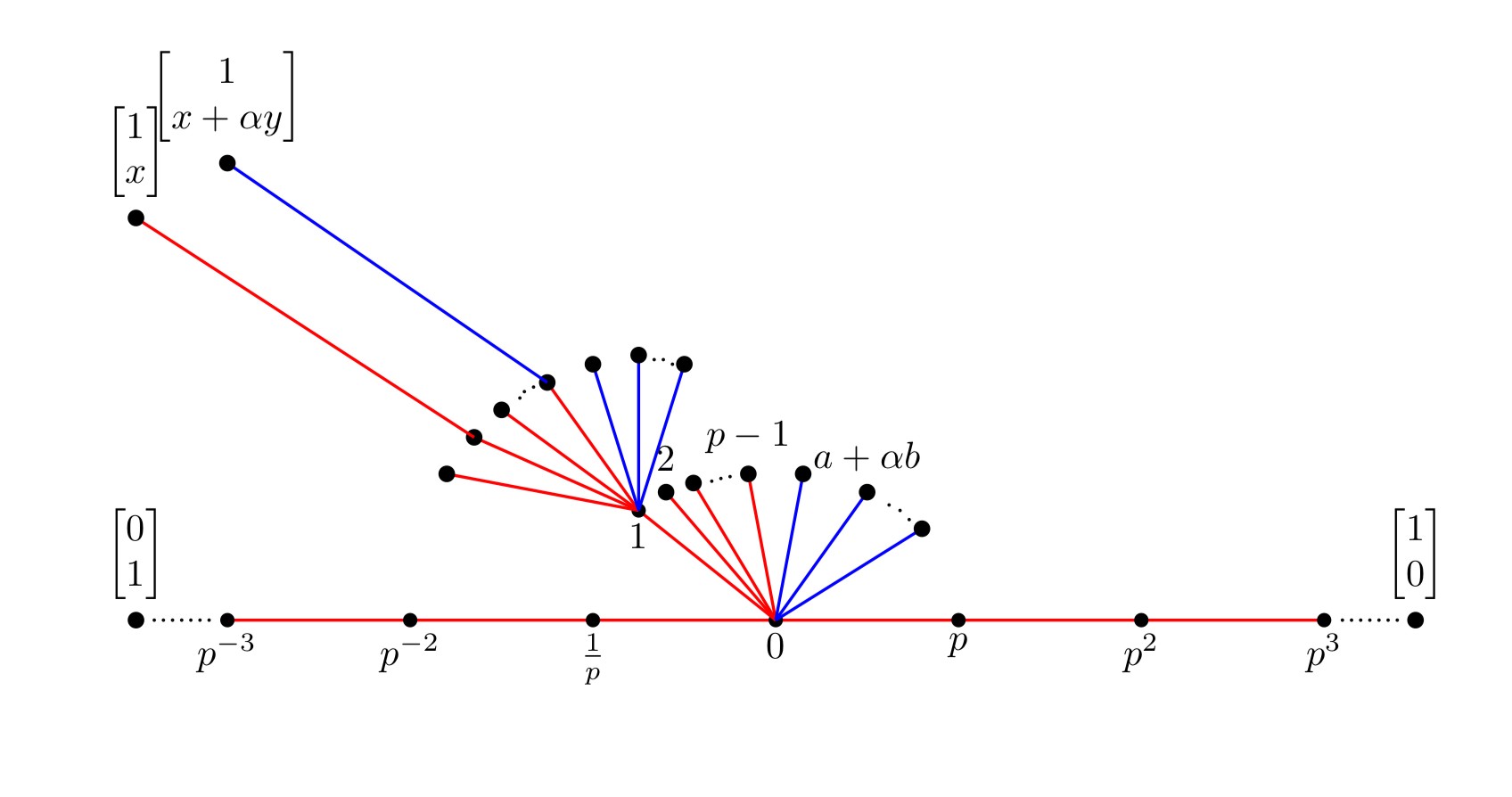
Figure 1. Unramified quadratic extension: Let $E={\mathbb{Q}}_{p}(\alpha)$ where $\alpha^{2}=S_{p}$ and $\alpha\not\in{\mathbb{Q}}_{p}$. In the tree for $\operatorname{SL}(2,{\mathbb{Q}}_{p})$ every vertex has $p+1$ neighbors. In the tree for $\operatorname{SL}(2,E)$ every vertex has $p^{2}+1$ neighbors, obtained by adding more edges (blue) to each vertex of the tree for $\operatorname{SL}(2,{\mathbb{Q}}_{p})$. We denote $a\in{\mathbb{F}}_{p}$ , $b\in{\mathbb{F}}_{p}^{*}$.

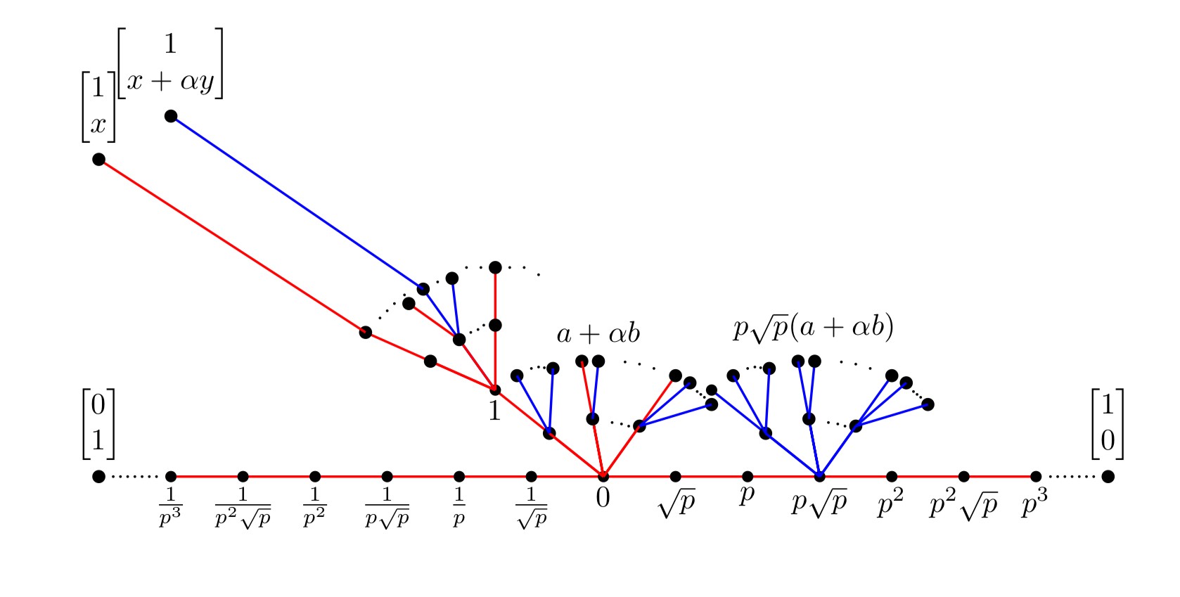
Figure 2. Ramified quadratic extension: Let $E={\mathbb{Q}}_{p}(\alpha)$ where $\alpha^{2}\in\{p,pS_{p}\}$ and $\alpha\not\in{\mathbb{Q}}_{p}$. In the tree for $\operatorname{SL}(2,{\mathbb{Q}}_{p})$ every vertex has $p+1$ neighbors. In the tree for $\operatorname{SL}(2,E)$ every vertex also has $p+1$ neighbors, obtained by adding $p+1$ blue edges from a vertex in the middle of each red edge. We denote $a\in{\mathbb{F}}_{p}^{*}$, $b\in{\mathbb{F}}_{p}$.

In the next few paragraphs we summarize results from [HW_class] for $k$-involutions of $\operatorname{SL}(2,k)$ when $k$ is a field of characteristic not equal to $2$. Let $\overline{k}$ be the algebraic closure of $k$.

Recall, a mapping $\phi:\operatorname{SL}(2,\overline{k})\to\operatorname{SL}(2,\overline{k})$ is a $k$-automorphism (or equivalently, an automorphism defined over $k$) if $\phi$ is a bijective rational $k$-homomorphism whose inverse is also a rational $k$-homomorphism, [Hel_k_invol, Sec. 2.2]. When $k=\overline{k}$, a $k$-automorphism $\phi$ is called an algebraic automorphism, or just an automorphism. To distinguish the terminology, an abstract automorphism of $\operatorname{SL}(2,\overline{k})$ is a bi-continuous isomorphism of $\operatorname{SL}(2,\overline{k})$ to itself, viewed as an abstract group.

An abstract automorphism $\theta$ of $\operatorname{SL}(2,\overline{k})$ of order two is an abstract involution of $\operatorname{SL}(2,\overline{k})$. A $k$-involution $\theta$ of $\operatorname{SL}(2,\overline{k})$ is a $k$-automorphism of $\operatorname{SL}(2,\overline{k})$ of order two, and the restriction of $\theta$ to $\operatorname{SL}(2,k)$ is a $k$-involution of $\operatorname{SL}(2,k)$. An abstract involution of $\operatorname{SL}(2,k)$ is an abstract automorphism of $\operatorname{SL}(2,k)$ of order two. Given $g\in\operatorname{SL}(2,\overline{k})$ denote by $\iota_{g}$ the inner automorphism of $\operatorname{SL}(2,\overline{k})$ defined by $x\mapsto\iota_{g}(x):=gxg^{-1}$.

The classification of the isomorphism classes of $k$-involutions of a connected reductive algebraic group defined over $k$ is given in [Hel_k_invol]. A simple characterization of the isomorphism classes of $k$-involutions of $\operatorname{SL}(n,k)$ is given in [HelWD]. We record the classification of $k$-involutions of $\operatorname{SL}(2,k)$:

Theorem 3.2.

[[HW_class] Theorem 1, Corollary 1, Corollary 2]. Every $k$-isomorphism class of $k$-involution of $\operatorname{SL}(2,k)$ is of the form $\iota_{A}$ with $A=\left(\begin{smallmatrix}0&1\\ a&0\end{smallmatrix}\right)\in\operatorname{GL}(2,k)$. Two such $k$-involutions $\iota_{A}$ with $A\in\{\left(\begin{smallmatrix}0&1\\ a&0\end{smallmatrix}\right),\left(\begin{smallmatrix}0&1\\ b&0\end{smallmatrix}\right)\}\subset\operatorname{GL}(2,k)$ of $\operatorname{SL}(2,k)$ are conjugate if and only if $a$ and $b$ are in the same square class of $k^{*}$. In particular, there are $order(k^{*}/(k^{*})^{2})$ $k$-isomorphism classes of $k$-involutions of $\operatorname{SL}(2,k)$.

Definition 3.3.

Given an involution $\theta$ of a group $G$ the fixed point group of $\theta$ is $H_{\theta}:=\{x\in G\;|\;\theta(x)=x\}$.

For $\theta$ a $k$-involution of $\operatorname{SL}(2,k)$ the quotient $\operatorname{SL}(2,k)/H_{\theta}$ is called a $k$-symmetric variety, and much of the structure of $\operatorname{SL}(2,k)/H_{\theta}$ is determined by $H_{\theta}$.

Proposition 3.4 ([HW_class] Section 3).

Let $\theta=\iota_{A}$, with $A=\left(\begin{smallmatrix}0&1\\ a&0\end{smallmatrix}\right)\in\operatorname{GL}(2,k)$, be a $k$-involution of $\operatorname{SL}(2,k)$. Then $H_{\theta}=\{\left(\begin{smallmatrix}x&y\\ ay&x\end{smallmatrix}\right)\in\operatorname{SL}(2,k)\;|\;x^{2}-ay^{2}=1\}$.

A quadratic form $q$ is isotropic if there exists a vector $x$ such that $q(x)=0$. Otherwise $q$ is anisotropic. In the context of groups, a non-compact subgroup $H_{\theta}$ will be called isotropic when $\theta$ is isotropic, and a bounded (or compact) subgroup $H_{\theta}$ will be called anisotropic when $\theta$ is anisotropic.

Theorem 3.5 ([HW_class] Section 3.2).

Let $k={\mathbb{Q}}_{p}$, $\theta=\iota_{A}$ with $A=\left(\begin{smallmatrix}0&1\\ a&0\end{smallmatrix}\right)$ and $\overline{a}\in{\mathbb{Q}}_{p}^{*}/({\mathbb{Q}}_{p}^{*})^{2}$. Then $H_{\theta}$ is anisotropic if and only if $\bar{a}\neq\bar{1}$. If $\bar{a}=\bar{1}$, then $H_{\theta}$ is isotropic and conjugate to the maximal ${\mathbb{Q}}_{p}$-split torus of $\operatorname{SL}(2,{\mathbb{Q}}_{p})$, i.e. the diagonal subgroup of $\operatorname{SL}(2,{\mathbb{Q}}_{p})$.

Remark 3.6.

In the case of $2\times 2$ matrices the operation inverse composed with transpose is given by an inner automorphism:

$$\left(\left(\begin{matrix}a&b\\ c&d\end{matrix}\right)^{T}\right)^{-1}=\left(\begin{matrix}a&c\\ b&d\end{matrix}\right)^{-1}=\left(\begin{matrix}d&-c\\ -b&a\end{matrix}\right)=\left(\begin{matrix}0&1\\ -1&0\end{matrix}\right)\left(\begin{matrix}a&b\\ c&d\end{matrix}\right)\left(\begin{matrix}0&-1\\ 1&0\end{matrix}\right).$$

This is not true for matrices of higher rank.

Finally, we link the ${\mathbb{Q}}_{p}$-involutions of $\operatorname{SL}(2,{\mathbb{Q}}_{p})$ given by Theorem 3.2 with quadratic forms over ${\mathbb{Q}}_{p}$.

Remark 3.7.

By [Serre, Corollary of Section 2.3], for $p\neq 2$, there are exactly 7 classes of quadratic forms of rank $2$ over ${\mathbb{Q}}_{p}$. We apply Remark 3.6. As $\left(\begin{smallmatrix}1&0\\ 0&-a\end{smallmatrix}\right)\left(\begin{smallmatrix}0&1\\ -1&0\end{smallmatrix}\right)=\left(\begin{smallmatrix}0&1\\ a&0\end{smallmatrix}\right)=:A\in\operatorname{GL}(2,{\mathbb{Q}}_{p})$, an involution $\theta=\iota_{A}$ of $\operatorname{SL}(2,{\mathbb{Q}}_{p})$ is determined by the quadratic form associated to the symmetric matrix $A$

$$\iota_{A}(g)=AgA^{-1}=\left(\begin{matrix}1&0\\ 0&-a\end{matrix}\right)(g^{-1})^{T}\left(\begin{matrix}1&0\\ 0&-a\end{matrix}\right)^{-1}$$

for every $g\in\operatorname{SL}(2,{\mathbb{Q}}_{p})$.

For $\operatorname{SL}(n,{\mathbb{Q}}_{p})$, with $n\geq 3$, the number of ${\mathbb{Q}}_{p}$-involutions is strictly larger than the number of the quadratic forms of rank $n$ over ${\mathbb{Q}}_{p}$, the latter is given by outer ${\mathbb{Q}}_{p}$-involutions (see [HelWD, Section 4.1.7, Section 6]).

4. Automorphisms and abstract automorphisms of $\operatorname{SL}(2,{\mathbb{Q}}_{p}(\alpha))$

Let $k$ be a local field of characteristic not equal to $2$ and denote by $\overline{k}$ the algebraic closure of $k$. The group of $k$-automorphisms of $\operatorname{SL}(2,\overline{k})$ is denoted by $\mathrm{Aut}_{k}(\operatorname{SL}(2,\overline{k}))$. If $k=\overline{k}$ then we just write $\mathrm{Aut}(\operatorname{SL}(2,\overline{k}))$, see [Hel_k_invol, Sec. 2.2], and those are called algebraic automorphisms, or just automorphisms, of $\operatorname{SL}(2,\overline{k})$.

Denote the group of inner automorphisms of $\operatorname{SL}(2,\overline{k})$ by $\operatorname{Inn}(\operatorname{SL}(2,\overline{k}))$ and the group of inner $k$-automorphisms of $\operatorname{SL}(2,\overline{k})$ by $\operatorname{Inn}_{k}(\operatorname{SL}(2,\overline{k}))$. Then $\operatorname{Inn}_{k}(\operatorname{SL}(2,\overline{k}))=\operatorname{Inn}(\operatorname{SL}(2,\overline{k}))\cap\mathrm{Aut}_{k}(\operatorname{SL}(2,\overline{k}))$, see [Hel_k_invol, Sec. 2.2].

By Borel [Bo] we have $\mathrm{Aut}(\operatorname{SL}(2,\overline{k}))=\operatorname{Inn}(\operatorname{SL}(2,\overline{k}))$.

We denote by $\mathrm{Aut}_{{\color[rgb]{0,0,0}\mathrm{abstrc}}}(\operatorname{SL}(2,\overline{k}))$ the group of all abstract automorphisms of $\operatorname{SL}(2,\overline{k})$ (see the terminology introduced just above Theorem 3.2), and by $\mathrm{Aut}(k)$ the group of all bi-continuous field automorphisms of $k$.

Abstract (bi-continuous) automorphisms of the $k$-rational points $G(k)$ of an absolutely almost simple algebraic group $G$ defined over an infinite field $k$ were described by Borel–Tits [BoTi], and also by Steinberg [Stein]. For example, the group $\operatorname{SL}(n,k)$ is an absolutely almost simple, simply connected group, and splits over $k$.

By those results, for $G$ as mentioned above, we have that $\mathrm{Aut}_{{\color[rgb]{0,0,0}\mathrm{abstrc}}}(G(k))$ fits in the exact sequence

$$1\to\mathrm{Aut}_{k}(G)\to\mathrm{Aut}_{{\color[rgb]{0,0,0}\mathrm{abstrc}}}(G(k))\to\mathrm{Aut}(k).$$

Let $\mathrm{Aut}_{G}(k)$ be the image of $\mathrm{Aut}_{{\color[rgb]{0,0,0}\mathrm{abstrc}}}(G(k))$ in $\mathrm{Aut}(k)$. When $G$ is a $k$-split connected reductive group, then $\mathrm{Aut}(k)=\mathrm{Aut}_{G}(k)$. And when $G$ is $k$-split, $\mathrm{Aut}_{{\color[rgb]{0,0,0}\mathrm{abstrc}}}(G(k))$ splits as the semi-direct product $\mathrm{Aut}_{k}(G)\rtimes\mathrm{Aut}_{G}(k)$, (see [BCL, Section 9.1], [Stu, Introduction]).

Thus, for the particular case of $\operatorname{SL}(2,k)$ we have that $\mathrm{Aut}_{{\color[rgb]{0,0,0}\mathrm{abstrc}}}(\operatorname{SL}(2,k))=\mathrm{Aut}_{k}(\operatorname{SL}(2,\overline{k}))\rtimes\mathrm{Aut}(k)$. In [Hel_k_invol, HW_class] only $k$-involutions of $\operatorname{SL}(2,k)$ are studied, i.e. involutions in $\mathrm{Aut}_{k}(\operatorname{SL}(2,\overline{k}))$.

In order to obtain all abstract involutions of $\operatorname{SL}(2,k)$, thus involutions in $\mathrm{Aut}_{{\color[rgb]{0,0,0}\mathrm{abstrc}}}(\operatorname{SL}(2,k))$, it remains to compute $\mathrm{Aut}(k)$ and then to combine with the $k$-automorphisms.

For $k={\mathbb{Q}}_{p}$, by [Con] we have $\mathrm{Aut}({\mathbb{Q}}_{p})=\{\operatorname{Id}\}$, and so for $\operatorname{SL}(2,{\mathbb{Q}}_{p})$ we have only ${\mathbb{Q}}_{p}$-involutions and those are computed by the results in [HW_class] recalled in Section 3 above.

For $k=E={\mathbb{Q}}_{p}(\alpha)$ a quadratic extension of ${\mathbb{Q}}_{p}$, to compute all the abstract involutions of $\operatorname{SL}(2,E)$, we compute $\mathrm{Aut}(E)$ and then combine it with $\mathrm{Aut}_{E}(\operatorname{SL}(2,\overline{{\mathbb{Q}}_{p}}))$ in order to obtain all abstract involutions of $\operatorname{SL}(2,E)$.

Definition 4.1.

Let $k$ be a local field and $K$ a finite field-extension of $k$. Let $\theta,\Psi\in\mathrm{Aut}_{{\color[rgb]{0,0,0}\mathrm{abstrc}}}(\operatorname{SL}(2,k))$. We say that $\theta$ and $\Psi$ are $\operatorname{GL}(2,K)$-conjugate if there is $X\in\operatorname{Inn}(\operatorname{GL}(2,K))$, such that $X^{-1}\theta X=\Psi$. In particular, there is a matrix $A\in\operatorname{GL}(2,K)$, such that $X=\iota_{A}$, and this means $A^{-1}(\theta(AgA^{-1}))A=\Psi(g)$, for every $g\in\operatorname{SL}(2,k)$.

Lemma 4.2.

Let $E$ be a quadratic extension of ${\mathbb{Q}}_{p}$, so $E={\mathbb{Q}}_{p}(\alpha)$, where $\alpha\in E\setminus\{{\mathbb{Q}}_{p}\}$ and $\alpha^{2}\in{\mathbb{Q}}_{p}$. Then $\mathrm{Aut}(E)=\{\operatorname{Id},\sigma\}$ where $\sigma(a+\alpha b)=a-\alpha b$.

Proof.

From [Schm] we know that a field which is complete with respect to two inequivalent nontrivial norms (i.e., the two norms induce distinct non-discrete topologies) must be algebraically closed. A corollary is that a field which is complete with respect to a nontrivial norm and which is not algebraically closed has only one equivalence class of norm, $n$. So an automorphism $\sigma$ of $E$ induces a norm $n_{\sigma}(x):=n(\sigma(x))$. But then $n_{\sigma}$ must be equivalent to the unique norm $n$, so $n_{\sigma}$ is some scalar multiple of $n$. Thus every automorphism of $E$ is continuous on $E$ with respect to the norm topology. Since ${\mathbb{Q}}$ is dense in ${\mathbb{Q}}_{p}$ and because any automorphism of $E$ is continuous and the identity on ${\mathbb{Q}}$, one can deduce that any automorphism on $E$ is trivial on ${\mathbb{Q}}_{p}$, thus Galois. Now as $\alpha^{2}\in{\mathbb{Q}}_{p}$, we have that any automorphism of $E$ will send $\alpha$ to $\pm\alpha$. Therefore $\mathrm{Aut}(E)=\{\operatorname{Id},\sigma\}$, where $\sigma:{\mathbb{Q}}_{p}(\alpha)\to{\mathbb{Q}}_{p}(\alpha)$, with $x\in{\mathbb{Q}}_{p}\mapsto\sigma(x)=x$, and $\alpha\mapsto\sigma(\alpha)=-\alpha$. ∎

Remark 4.3.

Let $k$ be a local field. By the results of Borel–Tits [BoTi] that are recalled in [BCL, Theorem 9.1 v)] we know that $\mathrm{Aut}_{{\color[rgb]{0,0,0}\mathrm{abstrc}}}(\operatorname{SL}(2,k))$ acts continuously, properly and faithfully on the Bruhat–Tits tree of $\operatorname{SL}(2,k)$. In the particular case when $k=E$ is a quadratic extension of ${\mathbb{Q}}_{p}$, the involution $\sigma$ is an automorphism of the Bruhat–Tits tree of $\operatorname{SL}(2,E)$, as well as any abstract involution $\theta$ of $\operatorname{SL}(2,E)$.

Let us now compute the abstract involutions of $\operatorname{SL}(2,E)$. If $A\in\operatorname{SL}(2,E)$ is a matrix and $\gamma\in\mathrm{Aut}(E)$ is a field automorphism, then $\gamma(A)$ is the matrix where $\gamma$ is applied to every matrix entry.

Theorem 4.4.

Let $E={\mathbb{Q}}_{p}(\alpha)$ be a quadratic extension of ${\mathbb{Q}}_{p}$. Then any abstract involution $\theta$ of $\operatorname{SL}(2,E)$ is of the form $\theta=\iota_{A}\circ\gamma$ where:

1. either $\gamma=\sigma$ and $A\in{\color[rgb]{0,0,0}\left\{\left(\begin{smallmatrix}z&y\\ 1&-\sigma(z)\end{smallmatrix}\right),\left(\begin{smallmatrix}x&0\\ 0&1\end{smallmatrix}\right)\right\}}\subset\operatorname{GL}(2,E)$, with $y\in{\mathbb{Q}}_{p},z,x\in E$, with $z\sigma(z)+y\neq 0$ and $x\sigma(x)=1,$

2. or $\gamma=\operatorname{Id}$ and $A$ is $\operatorname{SL}(2,E)$-conjugate to a matrix of the form $\left(\begin{smallmatrix}0&1\\ a&0\end{smallmatrix}\right)$, with $a\in E^{*}/(E^{*})^{2}$.

Proof.

By Borel–Tits [BoTi] any abstract automorphism of $\operatorname{SL}(2,E)$ is written as $\beta\circ\gamma$, with $\beta\in\mathrm{Aut}_{E}(\operatorname{SL}(2,\overline{{\mathbb{Q}}_{p}}))$ and $\gamma\in\mathrm{Aut}(E)=\{\operatorname{Id},\sigma\}$. By [HW_class, Remark 2] every $E$-automorphism of $\operatorname{SL}(2,E)$ can be written as the restriction to $\operatorname{SL}(2,E)$ of a inner automorphism of $\operatorname{GL}(2,E)$. Thus, given $\theta$ an abstract automorphism of $\operatorname{SL}(2,E)$ there exists $A=\left(\begin{smallmatrix}a&b\\ c&d\end{smallmatrix}\right)\in\operatorname{GL}(2,E)$ such that $\theta=\iota_{A}\circ\gamma$. From now on assume that $\theta$ is an abstract involution, thus $\theta^{2}=\operatorname{Id}$. Then, by [HW_class, Lemma 2], $A\gamma(A)=\left(\begin{smallmatrix}a\gamma(a)+b\gamma(c)&a\gamma(b)+b\gamma(d)\\ c\gamma(a)+d\gamma(c)&c\gamma(b)+d\gamma(d)\end{smallmatrix}\right)=q\operatorname{Id}$, for some $q\in E^{*}$, and with $\gamma\in\{\operatorname{Id},\sigma\}$. Thus we have

(1) $$a\gamma(a)+b\gamma(c)=c\gamma(b)+d\gamma(d)\qquad\text{and}\qquad c\gamma(a)+d\gamma(c)=0=a\gamma(b)+b\gamma(d).$$

When $\gamma=\operatorname{Id}$ we can directly apply the results of [HW_class, Section 1.3] and get that up to $\operatorname{SL}(2,E)$-conjugacy, $\theta=\iota_{A}$, with $A=\left(\begin{smallmatrix}0&1\\ t&0\end{smallmatrix}\right)$, with $t\in E^{*}/(E^{*})^{2}$.

We consider now the case $\gamma=\sigma$. By applying $\sigma$ to the second equality of (1) and putting together all four equations, we get

(2) $$a(\sigma(b)-\sigma(c))=\sigma(d)(c-b)\qquad\text{and}\qquad\sigma(a)(b-c)=d(\sigma(c)-\sigma(b)).$$

Case 1: If $a\neq 0$ then by (1) $d\neq 0$ and taking the ratio of the equations in (2) when it makes sense, or using the first equality of (1), gives $0\neq\frac{a}{d}=\frac{\sigma(d)}{\sigma(a)}{\color[rgb]{0,0,0}:=}x\in E$ , so $a=xd$ and $\sigma(d)=x\sigma(a)$. By applying $\sigma$, we have also $\sigma(a)=\sigma(x)\sigma(d)$. Then $\sigma(a)=\sigma(x)x\sigma(a)$ thus getting $\sigma(x)x=1$. Replacing $a$ by $xd$ in the first equality of (1) we get $b\sigma(c)=c\sigma(b)$.

If $c=b=0$ then $A=\left(\begin{smallmatrix}xd&0\\ 0&d\end{smallmatrix}\right)$, and modding out by the center one can just take $A=\left(\begin{smallmatrix}x&0\\ 0&1\end{smallmatrix}\right)$. Then one can verify that indeed $A\sigma(A)=\left(\begin{smallmatrix}x\sigma(x)&0\\ 0&1\end{smallmatrix}\right)=q\operatorname{Id}$, implying $q=1$.

As $b\sigma(c)=c\sigma(b)$ is symmetric in $b$ and $c$, we consider next that $c\neq 0$, then $b=cy$, with $y\in E$. Replacing $b=cy$ in $b\sigma(c)=c\sigma(b)$ one gets $y=\sigma(y)$, so $y\in{\mathbb{Q}}_{p}$. Thus $A=\left(\begin{smallmatrix}xd&cy\\ c&d\end{smallmatrix}\right)$ and so

$$A\sigma(A)=\begin{pmatrix}d\sigma(d)+yc\sigma(c)&xdy\sigma(c)+cy\sigma(d)\\ c\sigma(xd)+d\sigma(c)&cy\sigma(c)+d\sigma(d)\end{pmatrix}=\begin{pmatrix}q&0\\ 0&q\end{pmatrix}$$

from which it follows

$$xd\sigma(c)=-c\sigma(d)\qquad d\sigma(d)+yc\sigma(c)=q,$$

implying $q\in{\mathbb{Q}}_{p}$, because $y\in{\mathbb{Q}}_{p}$. We have three equations

$$xd\sigma(c)=-c\sigma(d)\qquad\sigma(x)\sigma(d)c=-\sigma(c)d\qquad d\sigma(d)=q-yc\sigma(c).$$

As by our assumption $c\neq 0$ and $d\neq 0$ then $0\neq\frac{xd}{c}=\frac{-\sigma(d)}{\sigma(c)}=:z\in E$. Rewriting our equations to include $z$ we have

$$xd=zc\qquad\sigma(x)\sigma(d)=\sigma(z)\sigma(c)\qquad-\sigma(d)=\sigma(c)z\qquad-d=c\sigma(z).$$

Thus $-\sigma(x)z=\sigma(z)$ and we can write $\sigma(x)=\frac{-\sigma(z)}{z}$. Returning to $A$ and substituting from above $d=\frac{zc}{x}$, we have

$$A=\begin{pmatrix}xd&cy\\ c&d\end{pmatrix}=\begin{pmatrix}x\frac{zc}{x}&cy\\ c&\frac{zc}{x}\end{pmatrix}=c\begin{pmatrix}z&y\\ 1&-\sigma(z)\end{pmatrix}.$$

And returning to our computation for $A\sigma(A)$ and taking $q^{\prime}:=\frac{q}{c\sigma(c)}\in{\mathbb{Q}}_{p}$ one can verify that indeed

$$\frac{1}{c\sigma(c)}A\sigma(A)=\begin{pmatrix}z\sigma(z)+y&0\\ 0&y+\sigma(z)z\end{pmatrix}=\begin{pmatrix}{\color[rgb]{0,0,0}q^{\prime}}&0\\ 0&{\color[rgb]{0,0,0}q^{\prime}}\end{pmatrix},\qquad q,y\in{\mathbb{Q}}_{p}.$$

Notice that the case $b=0$ follows from the case when $c\neq 0$ and $b=cy$ by taking $y=0$. This completes the proof if $a\neq 0$.

Case 2: If $a=0$ then $d=0$, and $A=\left(\begin{smallmatrix}0&b\\ c&0\end{smallmatrix}\right)$, and from (1) $b\sigma(c)=c\sigma(b)$. So $\frac{b}{c}=\frac{\sigma(b)}{\sigma(c)}=:y\neq 0$, and thus $y\in{\mathbb{Q}}_{p}^{*}$. Then $A=\left(\begin{smallmatrix}0&cy\\ c&0\end{smallmatrix}\right)$, reducing to $A=\left(\begin{smallmatrix}0&y\\ 1&0\end{smallmatrix}\right)$ with $y\in{\mathbb{Q}}_{p}^{*}$. ∎

Now we compute the fixed point groups of the involutions from Theorem 4.4 using the ends of the Bruhat–Tits tree of $\operatorname{SL}(2,K)$, where $K$ is a finite field-extension of $E$, and thus of ${\mathbb{Q}}_{p}$, that is chosen suitably. We will show those fixed point groups are either trivial, or compact, or $\operatorname{GL}(2,E)$-conjugate to either the diagonal subgroup in $\operatorname{SL}(2,E)$, or to $\operatorname{SL}(2,{\mathbb{Q}}_{p})$. Recall $E={\mathbb{Q}}_{p}(\alpha)$ is a quadratic extension of ${\mathbb{Q}}_{p}$ and $\mathcal{O}_{E}$ denotes the ring of integers of $E$.

We start with some easy lemmas.

Lemma 4.5.

Let $X\in\operatorname{SL}(2,E)$, or $X\in\operatorname{GL}(2,E)$. Let $\theta=\iota_{A}\circ\sigma$ be an abstract involution of $\operatorname{SL}(2,E)$, with $A\in\operatorname{GL}(2,E)$ as in Theorem 4.4. Then $\iota_{X^{-1}}\circ\theta\circ\iota_{X}=\sigma$ if and only if $A\sigma(X)=qX$, for some $q\in E^{*}$.

Proof.

By writing the equality $\iota_{X^{-1}}\theta\iota_{X}=\sigma$, we have

$$\begin{split}\sigma(g)&=\iota_{X^{-1}}\theta\iota_{X}(g)=X^{-1}(A(\sigma(XgX^{-1}))A^{-1})X=X^{-1}A\sigma(X)\sigma(g)\sigma(X^{-1})A^{-1}X\\ &=\iota_{X^{-1}A\sigma(X)}(\sigma(g)),\text{ for every }g\in\operatorname{SL}(2,E).\end{split}$$

Then by [HW_class, Lemma 2], we have $X^{-1}A\sigma(X)=q\operatorname{Id}$ for some $q\in E^{*}$. The converse implication is trivial. ∎

Definition 4.6.

Let $T_{d}$ be a $d$-regular tree with $d\geq 3$. Denote by $\partial T_{d}$ the visual boundary or ends which are identified for $T_{d}$. An automorphism $\theta_{1}\in\mathrm{Aut}(T_{d})$ is a tree-involution if $\theta_{1}^{2}=\operatorname{Id}\in\mathrm{Aut}(T_{d})$, in particular $\theta_{1}$ is an elliptic automorphism of $T_{d}$.

We denote by ${\color[rgb]{0,0,0}\mathrm{Fix}}_{T_{d}}(\theta_{1}):=\{v\in T_{d}\;|\;\theta_{1}(v)=v\}$, and by ${\color[rgb]{0,0,0}\mathrm{Fix}}_{\partial T_{d}}(\theta_{1}):=\{\xi\in\partial T_{d}\;|\;\theta_{1}(\xi)=\xi\}$. Notice, ${\color[rgb]{0,0,0}\mathrm{Fix}}_{T_{d}}(\theta_{1})$ is a (finite or infinite) connected subtree of $T_{d}$, and when the latter is infinite, we have ${\color[rgb]{0,0,0}\mathrm{Fix}}_{\partial T_{d}}(\theta_{1})\subseteq\partial{\color[rgb]{0,0,0}\mathrm{Fix}}_{T_{d}}(\theta_{1})$.

Also, consider the following two subgroups of $\mathrm{Aut}(T_{d})$:

$$\mathrm{Stab}_{\mathrm{Aut}(T_{d})}({\color[rgb]{0,0,0}\mathrm{Fix}}_{T_{d}}(\theta_{1})):=\{g\in\mathrm{Aut}(T_{d})\;|\;g({\color[rgb]{0,0,0}\mathrm{Fix}}_{T_{d}}(\theta_{1}))={\color[rgb]{0,0,0}\mathrm{Fix}}_{T_{d}}(\theta_{1})\text{ setwise}\}\text{ and }$$

$$\mathrm{Stab}_{\mathrm{Aut}(T_{d})}({\color[rgb]{0,0,0}\mathrm{Fix}}_{\partial T_{d}}(\theta_{1})):=\{g\in\mathrm{Aut}(T_{d})\;|\;g({\color[rgb]{0,0,0}\mathrm{Fix}}_{\partial T_{d}}(\theta_{1}))={\color[rgb]{0,0,0}\mathrm{Fix}}_{\partial T_{d}}(\theta_{1})\text{ setwise}\}.$$

If moreover ${\color[rgb]{0,0,0}\mathrm{Fix}}_{\partial T_{d}}(\theta_{1})$ is not the empty set we have

$$\mathrm{Stab}_{\mathrm{Aut}(T_{d})}({\color[rgb]{0,0,0}\mathrm{Fix}}_{T_{d}}(\theta_{1}))\leq\mathrm{Stab}_{\mathrm{Aut}(T_{d})}({\color[rgb]{0,0,0}\mathrm{Fix}}_{\partial T_{d}}(\theta_{1}))\text{ but they might not be equal.}$$

Lemma 4.7.

Let $K$ be a finite field-extension of ${\mathbb{Q}}_{p}$. Let $\theta$ be an abstract involution of $\operatorname{SL}(2,K)$, and let $H_{\theta}:=\{g\in\operatorname{SL}(2,K)\;|\;\theta(g)=g\}$. Let $\theta_{1}$ be the automorphism of the Bruhat–Tits tree $T_{K}$ of $\operatorname{SL}(2,K)$ induced by $\theta$. Then $\theta_{1}$ is a tree-involution of $T_{K}$ and

$$H_{\theta}\leq\mathrm{Stab}_{\mathrm{Aut}(T_{K})}({\color[rgb]{0,0,0}\mathrm{Fix}}_{T_{K}}(\theta_{1}))\leq\mathrm{Stab}_{\mathrm{Aut}(T_{K})}({\color[rgb]{0,0,0}\mathrm{Fix}}_{\partial T_{K}}(\theta_{1})).$$

Proof.

Since $\theta^{2}=\operatorname{Id}$, and by Remark 4.3 we have that $\theta_{1}^{2}=\operatorname{Id}$, thus $\theta_{1}$ is an involution in $\mathrm{Aut}(T_{K})$ as claimed, and in particular an elliptic automorphism of $T_{K}$.

Take now $g\in H_{\theta}$ and $x\in{\color[rgb]{0,0,0}\mathrm{Fix}}_{T_{K}}(\theta_{1})$. Then $\theta_{1}(g(x))=\theta(g)(\theta_{1}(x))=g(x)$, and thus $g(x)\in{\color[rgb]{0,0,0}\mathrm{Fix}}_{T_{K}}(\theta_{1})$, implying that $g\in\mathrm{Stab}_{\mathrm{Aut}(T_{K})}({\color[rgb]{0,0,0}\mathrm{Fix}}_{T_{K}}(\theta_{1}))$ and the conclusion follows. ∎

We first want to understand the case of the involution $\theta=\iota_{A}$ of $\operatorname{SL}(2,E)$ from Theorem 4.4 given by the matrix $A=\left(\begin{smallmatrix}0&1\\ a&0\end{smallmatrix}\right)$, with $a\in E^{*}/(E^{*})^{2}$. The fixed point group $H_{\theta}\leq\operatorname{SL}(2,E)$ of $\theta$ is computed in [HW_class]. We give a geometric interpretation of $H_{\theta}$ using the ends of the Bruhat–Tits tree of $\operatorname{SL}(2,K_{a})$, where $K_{a}:=E(\sqrt{a})$ is a quadratic extension of $E$. The ends of the tree $T_{K_{a}}$ are the elements of the projective space $P^{1}K_{a}=\big{[}\begin{smallmatrix}0\\ 1\end{smallmatrix}\big{]}\bigsqcup\limits_{x\in K_{a}}\big{[}\begin{smallmatrix}1\\ x\end{smallmatrix}\big{]}$. Notice, the action of $\theta=\iota_{A}$ on the Bruhat–Tits tree (and its boundary) of $\operatorname{SL}(2,E)$, and respectively of $\operatorname{SL}(2,K_{a})$, is the automorphism induced by $A\in\operatorname{GL}(2,E){\color[rgb]{0,0,0}\leq\mathrm{Aut}(T_{E})}$ on the trees and their respective boundaries. For example, for $A=\left(\begin{matrix}x&y\\ z&t\end{matrix}\right)\in\operatorname{GL}(2,E)$ and $\xi=\big{[}\begin{smallmatrix}c\\ d\end{smallmatrix}\big{]}\in P^{1}E$ an end, $A(\xi)=\left(\begin{matrix}x&y\\ z&t\end{matrix}\right)\big{[}\begin{smallmatrix}c\\ d\end{smallmatrix}\big{]}=\big{[}\begin{smallmatrix}xc+yd\\ zc+td\end{smallmatrix}\big{]}$.

Given $X\subset P^{1}K$, we denote by ${\color[rgb]{0,0,0}\mathrm{Fix}}_{\operatorname{SL}(2,K)}(X):=\{g\in\operatorname{SL}(2,K)\;|\;g(x)=x,\forall x\in X\}$ the set of elements in $\operatorname{SL}(2,K)$ fixing $X$ pointwise.

Corollary 4.8.

Let $F$ be a finite field-extension of ${\mathbb{Q}}_{p}$, $A=\left(\begin{smallmatrix}0&1\\ a&0\end{smallmatrix}\right)$, with $a\in F^{*}/(F^{*})^{2}$, and $\theta_{a}:=\iota_{A}$ the corresponding $F$-involution of $\operatorname{SL}(2,F)$. Take $K_{a}:=F(\sqrt{a})$ a quadratic field extension. Then the only solutions of the equation $A(\xi)=\xi$ with $\xi\in P^{1}K_{a}$ are $\xi_{\pm}:=\big{[}\begin{smallmatrix}1\\ \pm\sqrt{a}\end{smallmatrix}\big{]}$ and $H_{\theta_{a}}={\color[rgb]{0,0,0}\mathrm{Fix}}_{\operatorname{SL}(2,K_{a})}(\{\xi_{-},\xi_{+}\})\cap\operatorname{SL}(2,F)=\{\left(\begin{smallmatrix}x&y\\ ay&x\end{smallmatrix}\right)\in\operatorname{SL}(2,F)\;|\;x^{2}-ay^{2}=1\}$. Moreover,

1. if $a=1$ then $\xi_{\pm}:=\big{[}\begin{smallmatrix}1\\ \pm 1\end{smallmatrix}\big{]}$ and $H_{\theta_{a}}$ contains all the hyperbolic elements of $\operatorname{SL}(2,F)$ with $\xi_{\pm}$ as their repelling and attracting endpoints. In particular, $H_{\theta_{a}}$ is $\operatorname{GL}(2,F)$-conjugate to the entire diagonal subgroup of $\operatorname{SL}(2,F)$, thus $H_{\theta_{a}}$ is noncompact and abelian.

2. if $a\neq 1$ then $\xi_{\pm}:=\big{[}\begin{smallmatrix}1\\ \pm\sqrt{a}\end{smallmatrix}\big{]}\in P^{1}K_{a}-P^{1}F$, and $H_{\theta_{a}}$ is compact and abelian.

Proof.

We search for all the ends $\xi\in P^{1}K_{a}$ such that $A(\xi)=\xi$. This means that we search for all vectors $\big{(}\begin{smallmatrix}1\\ x\end{smallmatrix}\big{)}$ with $x\in K_{a}$, or $\big{(}\begin{smallmatrix}0\\ 1\end{smallmatrix}\big{)}$, such that:

$$\left(\begin{matrix}0&1\\ a&0\end{matrix}\right)\begin{pmatrix}1\\ x\end{pmatrix}=c\begin{pmatrix}1\\ x\end{pmatrix}{\color[rgb]{0,0,0}\textrm{i.e.,}}\begin{pmatrix}x\\ a\end{pmatrix}=\begin{pmatrix}c\\ cx\end{pmatrix}\qquad\textrm{or}\qquad\left(\begin{matrix}0&1\\ a&0\end{matrix}\right)\begin{pmatrix}0\\ 1\end{pmatrix}=c\begin{pmatrix}0\\ 1\end{pmatrix}{\color[rgb]{0,0,0}\textrm{i.e.,}}\begin{pmatrix}1\\ 0\end{pmatrix}=\begin{pmatrix}0\\ c\end{pmatrix}$$

for some $c\in K_{a}^{*}$. One can see that the only solutions are given by $c=x$ and $a=c^{2}$, implying that $\xi_{\pm}:=\big{[}\begin{smallmatrix}1\\ \pm\sqrt{a}\end{smallmatrix}\big{]}\in P^{1}K_{a}=P^{1}F(\sqrt{a})$ are the only solutions of the equation $A(\xi)=\xi$.

Next, we claim that the involution $\theta_{a}=\iota_{A}$ is $\operatorname{GL}(2,K_{a})$-conjugate to the involution $\iota_{B}$ of $\operatorname{SL}(2,K_{a})$, where $B:=\left(\begin{smallmatrix}1&0\\ 0&-1\end{smallmatrix}\right)$. Indeed, taking

$$C:=\left(\begin{matrix}1&-\frac{1}{\sqrt{a}}\\ \sqrt{a}&1\end{matrix}\right)\in\operatorname{GL}(2,K_{a})\qquad\textrm{{\color[rgb]{0,0,0}leads to}}\qquad\iota_{C^{-1}}\circ\theta_{a}\circ\iota_{C}=\iota_{C^{-1}AC}=\iota_{B}.$$

It is easy to see that the fixed point group in $\operatorname{SL}(2,K_{a})$ of the involution $\iota_{B}$ is ${\color[rgb]{0,0,0}\mathrm{Diag}}(2,K_{a})$, the full diagonal subgroup of $\operatorname{SL}(2,K_{a})$. Thus, from above, the fixed point group in $\operatorname{SL}(2,K_{a})$ of the involution $\iota_{A}$ is the subgroup

$${\color[rgb]{0,0,0}\mathrm{Fix}}_{\operatorname{SL}(2,K_{a})}(\{\xi_{-},\xi_{+}\})=C{\color[rgb]{0,0,0}\mathrm{Diag}}(2,K_{a})C^{-1}\leq\operatorname{SL}(2,K_{a})$$

which is the stabilizer in $\operatorname{SL}(2,K_{a})$ of the bi-infinite geodesic line $[\xi_{-},\xi_{+}]$ in the Bruhat–Tits tree $T_{K_{a}}\cup\partial T_{K_{a}}$, and fixes pointwise the two ends $\xi_{-},\xi_{+}$. Then $H_{\theta_{a}}={\color[rgb]{0,0,0}\mathrm{Fix}}_{\operatorname{SL}(2,K_{a})}(\{\xi_{-},\xi_{+}\})\cap\operatorname{SL}(2,F)$.

Notice, the geodesic line $[\xi_{-},\xi_{+}]$ appears in the Bruhat–Tits tree $T_{F}\cup\partial T_{F}$ if and only if $a=1$. The rest of the Corollary is an easy verification, and an application of Proposition 3.4. ∎

In the next few pages we will compute the fixed point groups $H_{\theta}$ for abstract involutions $\theta=\iota_{A}\circ\sigma$ from Theorem 4.4. We will show:

Theorem 4.9.

Let $E={\mathbb{Q}}_{p}(\alpha)$ be a quadratic extension of ${\mathbb{Q}}_{p}$. Consider any abstract involution $\theta=\iota_{A}\circ\sigma$ of $\operatorname{SL}(2,E)$ as in Theorem 4.4, where $A\in\{\left(\begin{smallmatrix}z&y\\ 1&-\sigma(z)\end{smallmatrix}\right),\left(\begin{smallmatrix}x&0\\ 0&1\end{smallmatrix}\right)\}\subset\operatorname{GL}(2,E)$, with $y\in{\mathbb{Q}}_{p},z,x\in E$, with $z\sigma(z)+y\neq 0$ and $x\sigma(x)=1$. Then one of the following holds for $H_{\theta}:=\{g\in\operatorname{SL}(2,E)\;|\;\theta(g)=g\}$:

1. $H_{\theta}$ is $\operatorname{GL}(2,E)$-conjugate to $\operatorname{SL}(2,{\mathbb{Q}}_{p})$

2. $H_{\theta}=B\operatorname{SL}(2,K^{\sigma})B^{-1}\cap\operatorname{SL}(2,E)$, for some matrix $B\in\operatorname{GL}(2,K)$, where $K\neq E$ is some finite field-extension of $E$ and $K^{\sigma}:=\{x\in K\;|\;\sigma(x)=x\}$ is the maximal subfield of $K$ fixed by $\sigma$. In particular, $H_{\theta}$ is compact or trivial.

Proof.

Consider $\theta=\iota_{A}\circ\sigma$, with $A=\left(\begin{smallmatrix}x&0\\ 0&1\end{smallmatrix}\right)$ and where $x=x_{1}+{\color[rgb]{0,0,0}\alpha}x_{2}\in E={\mathbb{Q}}_{p}(\alpha)$ such that $x\sigma(x)=1$. If $x=1$, then clearly $H_{\theta}=\operatorname{SL}(2,{\mathbb{Q}}_{p})$. If $x\neq 1$, there are two cases:

$$\begin{array}[]{cc}\textrm{Case 1: }{\color[rgb]{0,0,0}\textrm{Suppose }x=-1\textrm{ then }x_{1}=-1,x_{2}=0}&\textrm{Case 2: }{\color[rgb]{0,0,0}\textrm{Suppose }x\neq\pm 1\textrm{ then }x_{2}\neq 0}\\ {\color[rgb]{0,0,0}\textrm{and set }}B=\left(\begin{matrix}\alpha&0\\ 0&1\end{matrix}\right)&{\color[rgb]{0,0,0}\textrm{and set }}B=\left(\begin{matrix}\frac{x_{1}+1}{x_{2}}+\alpha&0\\ 0&1\end{matrix}\right)\end{array}.$$

Then in both cases we see that $\iota_{B^{-1}}\circ\theta\circ\iota_{B}=\iota_{B^{-1}A\sigma(B)}\circ\sigma=\sigma$, implying that $\theta=\iota_{A}\circ\sigma$ is $\operatorname{GL}(2,E)$-conjugate to $\sigma$ via the map $\iota_{B^{-1}}$. Thus in this case $H_{\theta}:=\{g\in\operatorname{SL}(2,E)\;|\;\theta(g)=g\}$ is $\operatorname{GL}(2,E)$-conjugate to $\operatorname{SL}(2,{\mathbb{Q}}_{p})$.

Finally, consider the general case from Theorem 4.4 where $\theta=\iota_{A}\circ\sigma$, with $A=\left(\begin{smallmatrix}z&y\\ 1&-\sigma(z)\end{smallmatrix}\right)$ and where $y\in{\mathbb{Q}}_{p},z\in E$ such that $z\sigma(z)+y\neq 0$. Recall that

(3) $$A\sigma(A)=c\operatorname{Id},\text{ for some }c\in E^{*}.$$

Notice, the action of $\sigma$ on the Bruhat–Tits tree of $\operatorname{SL}(2,E)$ is again the natural map induced by $\sigma$, as the vertices of $T_{E}$ can be labeled with $a+\alpha b$, where $a,b\in{\mathbb{Q}}_{p}$ (see Figures 1, 2). In other words, $\sigma$ induces an action on $T_{E}$ which fixes the subtree for $T_{{\mathbb{Q}}_{p}}$ and acts as an involution on the remaining branches in $T_{E}-T_{{\mathbb{Q}}_{p}}$. Then the involution $\theta_{1}$ of the Bruhat–Tits tree of $\operatorname{SL}(2,E)$ induced by the involution $\theta$ of $\operatorname{SL}(2,E)$ is just the map $\theta_{1}=A\circ\sigma$. The same involution $\theta_{1}=A\circ\sigma$ acts on the boundary $\partial T_{E}$ of $T_{E}$. Moreover, since $A\in\operatorname{GL}(2,E)$, the map $A$ acts on the $\partial T_{E}$ as an automorphism, and thus is a bijection on $\partial T_{E}$.

In order to classify the involutions $\theta$ up to $\operatorname{GL}(2,E)$-conjugacy, we first want to find solutions of the equation $\theta_{1}(\xi)=A(\sigma(\xi))=\xi$, with $\xi\in\partial T_{E}$, and use those solutions to find matrices $B\in\operatorname{GL}(2,E)$ with $A\sigma(B)=cB$ and $c\in E^{*}$. If there is no such solution, we will solve this equation for $\xi\in\partial T_{K}$, where $K$ is an appropriate finite extension of $E$. Notice that the actions of $A$ and $\sigma$ extend naturally to $T_{K}\cup\partial T_{K}$, with $\sigma$ fixing pointwise any primitive element in $K-E$. The action of $\sigma$ extends to $K$, since all the extensions are algebraic and we have ${\mathbb{Q}}_{p}\subset E\subset K$.

Putting together the above remarks, it is enough to find all the solutions of the equation $A(\sigma(A(\xi)))=A(\xi)$, for $\xi\in\partial T_{K}$ and $K$ a finite extension of $E$. Since $A(\sigma(A(\xi)))=A\sigma(A)(\sigma(\xi))=c\sigma(\xi)$ where $\xi\in P^{1}K=\big{[}\begin{smallmatrix}0\\ 1\end{smallmatrix}\big{]}\bigsqcup\limits_{x\in K}\big{[}\begin{smallmatrix}1\\ x\end{smallmatrix}\big{]}$ it is then equivalent to finding all the ${\color[rgb]{0,0,0}c^{\prime}}\in K^{*}$ and $x\in K$ such that

(4) $$\begin{pmatrix}1\\ \sigma(x)\end{pmatrix}={\color[rgb]{0,0,0}c^{\prime}}A\begin{pmatrix}1\\ x\end{pmatrix},\;\;\textrm{or}\;\;\begin{pmatrix}0\\ 1\end{pmatrix}={\color[rgb]{0,0,0}c^{\prime}}A\begin{pmatrix}0\\ 1\end{pmatrix}$$

where $K$ is an appropriate finite extension of $E$ that will be determined below. First notice that any element $x\in K$ can be uniquely written as $x=x_{1}+\alpha x_{2}$, with $x_{1},x_{2}$ elements in $K$ such that $\sigma(x_{i})=x_{i}$.

Thus, write

$$\left(\begin{matrix}z&y\\ 1&-\sigma(z)\end{matrix}\right)=A=A_{1}+\alpha A_{2}=\left(\begin{matrix}z_{1}&y\\ 1&-z_{1}\end{matrix}\right)+\alpha\left(\begin{matrix}z_{2}&0\\ 0&z_{2}\end{matrix}\right),{\color[rgb]{0,0,0}\textrm{ and }}\xi=\begin{bmatrix}x_{1}+\alpha x_{2}\\ y_{1}+\alpha y_{2}\end{bmatrix},$$

and $A_{1},A_{2}\in M_{2}({\mathbb{Q}}_{p})$, for $x_{1},x_{2},y_{1},y_{2}\in K$ such that $\sigma(x_{i})=x_{i}$, $\sigma(y_{i})=y_{i}$. Since we will have more flexibility by considering $\xi$ in its general form $\begin{bmatrix}x_{1}+\alpha x_{2}\\ y_{1}+\alpha y_{2}\end{bmatrix}$, we want to solve the equation for $\xi\in\partial T_{K}$ and $c\in K^{*}$ as in (3):

(5) $$c\begin{pmatrix}x_{1}-\alpha x_{2}\\ y_{1}-\alpha y_{2}\end{pmatrix}=(A_{1}+\alpha A_{2})\begin{pmatrix}x_{1}+\alpha x_{2}\\ y_{1}+\alpha y_{2}\end{pmatrix}=A_{1}\begin{pmatrix}x_{1}\\ y_{1}\end{pmatrix}+\alpha^{2}A_{2}\begin{pmatrix}x_{2}\\ y_{2}\end{pmatrix}+\alpha A_{1}\begin{pmatrix}x_{2}\\ y_{2}\end{pmatrix}+\alpha A_{2}\begin{pmatrix}x_{1}\\ y_{1}\end{pmatrix}$$

where $c=c_{1}+\alpha c_{2}\in K^{*}$ and $\sigma(c_{i})=c_{i}$. This equation (5) is equivalent to the following system of equations:

(6) $$(A_{1}-c_{1}\operatorname{Id})\begin{pmatrix}x_{1}\\ y_{1}\end{pmatrix}=-\alpha^{2}(z_{2}+c_{2})\begin{pmatrix}x_{2}\\ y_{2}\end{pmatrix},\;\;\;\;(A_{1}+c_{1}\operatorname{Id})\begin{pmatrix}x_{2}\\ y_{2}\end{pmatrix}=-(z_{2}-c_{2})\begin{pmatrix}x_{1}\\ y_{1}\end{pmatrix}.$$

Multiplying the second equality of (6) by $A-c_{1}\operatorname{Id}$ and using the first equality, we have:

(7) $$(A_{1}^{2}-c_{1}^{2}\operatorname{Id})\begin{pmatrix}x_{2}\\ y_{2}\end{pmatrix}=(z_{1}^{2}+y-c_{1}^{2})\begin{pmatrix}x_{2}\\ y_{2}\end{pmatrix}=\alpha^{2}(z_{2}^{2}-c_{2}^{2})\begin{pmatrix}x_{2}\\ y_{2}\end{pmatrix}.$$

We solve Equation (7) by breaking it into cases, by comparing when the coefficients $(z_{1}^{2}+y-c_{1}^{2})$ and $\alpha^{2}(z_{2}^{2}-c_{2}^{2})$ are equal to each other, or zero.

Case 1: If ${\color[rgb]{0,0,0}0\neq}z_{1}^{2}+y-c_{1}^{2}\neq\alpha^{2}(z_{2}^{2}-c_{2}^{2})\neq 0$ then we must have $\big{(}\begin{smallmatrix}x_{2}\\ y_{2}\end{smallmatrix}\big{)}=\big{(}\begin{smallmatrix}0\\ 0\end{smallmatrix}\big{)}$, and so also $\big{(}\begin{smallmatrix}x_{1}\\ y_{1}\end{smallmatrix}\big{)}=\big{(}\begin{smallmatrix}0\\ 0\end{smallmatrix}\big{)}$. Thus there is no solution $\xi\in\partial T_{K}$ for the system (6), for any finite extension $K$.

Case 2.1: If $z_{1}^{2}+y-c_{1}^{2}\neq 0$, $z_{2}^{2}-c_{2}^{2}=0$, and $z_{2}\neq 0\neq c_{2}$. Then $\big{(}\begin{smallmatrix}x_{2}\\ y_{2}\end{smallmatrix}\big{)}=\big{(}\begin{smallmatrix}0\\ 0\end{smallmatrix}\big{)}$. If moreover, $z_{2}=-c_{2}$, from (6) we get that $\big{(}\begin{smallmatrix}x_{1}\\ y_{1}\end{smallmatrix}\big{)}=\big{(}\begin{smallmatrix}0\\ 0\end{smallmatrix}\big{)}$. If instead $z_{2}=c_{2}$, from (6) we get that $(A_{1}-c_{1}\operatorname{Id})\big{(}\begin{smallmatrix}x_{1}\\ y_{1}\end{smallmatrix}\big{)}=\big{(}\begin{smallmatrix}0\\ 0\end{smallmatrix}\big{)}$ and because ${\color[rgb]{0,0,0}\mathrm{det}}(A_{1}-c_{1}\operatorname{Id})=-(z_{1}^{2}-c_{1}^{2}+y)\neq 0$ we also get $\big{(}\begin{smallmatrix}x_{1}\\ y_{1}\end{smallmatrix}\big{)}=\big{(}\begin{smallmatrix}0\\ 0\end{smallmatrix}\big{)}$. Thus in this Case 2 there is no solution $\xi\in\partial T_{K}$ for the system (6).

Case 2.2: If $z_{1}^{2}+y-c_{1}^{2}\neq 0$, and $z_{2}=0=c_{2}$. This means that $A_{2}=\left(\begin{smallmatrix}0&0\\ 0&0\end{smallmatrix}\right)$, and so $A=A_{1}=\left(\begin{smallmatrix}z_{1}&y\\ 1&-z_{1}\end{smallmatrix}\right)\in\operatorname{GL}(2,{\mathbb{Q}}_{p})$, with $A^{2}=(z_{1}^{2}+y)\operatorname{Id}$. The system of equations (6) reduces to

(8) $$(A_{1}-c_{1}\operatorname{Id})\begin{pmatrix}x_{1}\\ y_{1}\end{pmatrix}=\begin{pmatrix}0\\ 0\end{pmatrix},\;\;\;\;(A_{1}+c_{1}\operatorname{Id})\begin{pmatrix}x_{2}\\ y_{2}\end{pmatrix}=\begin{pmatrix}0\\ 0\end{pmatrix}.$$

As the matrices $(A_{1}-c_{1}\operatorname{Id})$ and $(A_{1}+c_{1}\operatorname{Id})$ are invertible, with determinant $-(z_{1}^{2}-c_{1}^{2}+y)\neq 0$, we get $\big{(}\begin{smallmatrix}x_{1}\\ y_{1}\end{smallmatrix}\big{)}=\big{(}\begin{smallmatrix}0\\ 0\end{smallmatrix}\big{)}=\big{(}\begin{smallmatrix}x_{2}\\ y_{2}\end{smallmatrix}\big{)}$. Again there is no solution $\xi\in\partial T_{K}$ for the system (6).

Case 3: If $z_{1}^{2}+y-c_{1}^{2}=0$ and $z_{2}^{2}-c_{2}^{2}\neq 0$. Then from (7) we get $\big{(}\begin{smallmatrix}x_{2}\\ y_{2}\end{smallmatrix}\big{)}=\big{(}\begin{smallmatrix}0\\ 0\end{smallmatrix}\big{)}$ and then from (6) $\big{(}\begin{smallmatrix}x_{1}\\ y_{1}\end{smallmatrix}\big{)}=\big{(}\begin{smallmatrix}0\\ 0\end{smallmatrix}\big{)}$. Again there is no solution $\xi\in\partial T_{K}$ for the system (6).

Thus the remaining cases to check for the coefficients that are not covered above is to solve for $\xi\in\partial T_{K}$ when:

1. $0\neq z_{1}^{2}+y-c_{1}^{2}=\alpha^{2}(z_{2}^{2}-c_{2}^{2})\neq 0$, and where we take $K$ to be the minimal field extension of ${\mathbb{Q}}_{p}$ that contains $c_{1},c_{2}$

2. $z_{2}^{2}=c_{2}^{2}$, thus for $c_{2}\in{\mathbb{Q}}_{p}$, and $z_{1}^{2}+y-c_{1}^{2}=0$ for some $c_{1}\in K$, where $K$ is a minimal extension of $E$ in which $z_{1}^{2}+y$ is a square.

In each of the Cases 4, 5.1, 5.2, 5.3, one checks $B_{i}\in\operatorname{GL}(2,K)$ since ${\color[rgb]{0,0,0}\mathrm{det}}(B_{i})\neq 0$ and also that $A\sigma(B_{i})=(c_{1}+\alpha c_{2})B_{i}=cB_{i}$.

Case 4: If $0\neq z_{1}^{2}+y-c_{1}^{2}=\alpha^{2}(z_{2}^{2}-c_{2}^{2})\neq 0$. Then take the matrix

$$B_{1}:=\left(\begin{matrix}\frac{y}{z_{2}-c_{2}}&\frac{z_{1}+c_{1}}{z_{2}-c_{2}}+\alpha\\ \frac{-z_{1}+c_{1}}{z_{2}-c_{2}}+\alpha&\frac{1}{z_{2}-c_{2}}\end{matrix}\right).$$

Case 5.1: If $z_{1}^{2}+y-c_{1}^{2}=0$, $z_{2}^{2}-c_{2}^{2}=0$, $y\neq 0$, and $z_{2}=c_{2}\neq 0$. Then take the matrix

$$B_{2}:=\left(\begin{matrix}-\frac{\alpha^{2}({\color[rgb]{0,0,0}2z_{2}})(z_{1}+c_{1})}{y}+\alpha&\alpha^{2}({\color[rgb]{0,0,0}2z_{2}})+(z_{1}+c_{1})+\alpha(z_{1}-c_{1})\\ -\frac{\alpha(z_{1}+c_{1})}{y}&1+\alpha\end{matrix}\right).$$

Case 5.2: If $z_{1}^{2}+y-c_{1}^{2}=0$, $z_{2}^{2}-c_{2}^{2}=0$, $y\neq 0$, and $z_{2}=-c_{2}\neq 0$. Then take the matrix

$${\color[rgb]{0,0,0}B_{3}:=\left(\begin{matrix}1+\alpha\frac{2z_{2}}{z_{1}+c_{1}}&(z_{1}+c_{1})-\alpha(z_{1}-c_{1}-2z_{2})\\ \frac{1}{z_{1}+c_{1}}&1-\alpha\end{matrix}\right).}$$

Case 5.3: If $z_{1}^{2}+y-c_{1}^{2}=0$, $z_{2}=c_{2}=0$, and $y\neq 0$. This means that $A_{2}=\left(\begin{smallmatrix}0&0\\ 0&0\end{smallmatrix}\right)$, and so $A=A_{1}=\left(\begin{smallmatrix}z_{1}&y\\ 1&-z_{1}\end{smallmatrix}\right)\in\operatorname{GL}(2,{\mathbb{Q}}_{p})$. Then take the matrix

$$B_{4}:=\left(\begin{matrix}\alpha(z_{1}-c_{1})&1\\ \alpha&\frac{c_{1}-z_{1}}{y}\end{matrix}\right).$$

Case 5.4: If $z_{1}^{2}-c_{1}^{2}=0$, $z_{2}^{2}-c_{2}^{2}=0$, and $y=0$. This means that $c=c_{1}+\alpha c_{2}\in E$ and $A=\left(\begin{smallmatrix}z&0\\ 1&-\sigma(z)\end{smallmatrix}\right)\in\operatorname{GL}(2,E)$. Since multiplication by a constant in $E^{*}$ will give the same results, we can multiply $A$ with $-\frac{1}{\sigma(z)}$, and we get a matrix $A=\left(\begin{smallmatrix}x&0\\ w&1\end{smallmatrix}\right)$ such that $x\sigma(x)=1$ and $w=-x\sigma(w)$, with $x,w\in E^{*}$.

By our assumption $z_{1}\neq 0$ or $z_{2}\neq 0$. There are a few final subcases, set $x=x^{\prime}_{1}+\alpha x^{\prime}_{2}$, and $w=w_{1}+\alpha w_{2}$:

$$\begin{array}[]{ccc}{\color[rgb]{0,0,0}\textrm{if }}z_{1}z_{2}\neq 0&{\color[rgb]{0,0,0}\textrm{then }}{\color[rgb]{0,0,0}x^{\prime}_{2}}\neq 0,w_{2}\neq 0&{\color[rgb]{0,0,0}\textrm{and take }}B_{5}:=\left(\begin{matrix}\frac{1+{\color[rgb]{0,0,0}x^{\prime}_{1}}}{{\color[rgb]{0,0,0}x^{\prime}_{2}}}+\alpha&0\\ \alpha\frac{w_{2}}{{\color[rgb]{0,0,0}x^{\prime}_{2}}}&1\end{matrix}\right)\\ &&\\ {\color[rgb]{0,0,0}\textrm{if }}z_{1}z_{2}=0&\textrm{and }x=1,{\color[rgb]{0,0,0}\textrm{ then }}w=\alpha w_{2}&{\color[rgb]{0,0,0}\textrm{take }}B_{5}:=\left(\begin{smallmatrix}1&0\\ \alpha\frac{w_{2}}{2}&1\end{smallmatrix}\right)\\ &&\\ {\color[rgb]{0,0,0}\textrm{if }}z_{1}z_{2}=0&\textrm{and }x=-1,{\color[rgb]{0,0,0}\textrm{ then }}w=w_{1}&{\color[rgb]{0,0,0}\textrm{take }}B_{5}:=\left(\begin{smallmatrix}\alpha&\alpha\\ 1-\alpha\frac{w_{1}}{2}&-1-\alpha\frac{w_{1}}{2}\end{smallmatrix}\right).\end{array}$$

In all those subcases we see $A\sigma(B_{5})=B_{5}$ and note ${\color[rgb]{0,0,0}\mathrm{det}}(B_{5})\neq 0$ in all cases.

In all the above cases we verified $\iota_{B_{i}^{-1}}\circ\theta\circ\iota_{B_{i}}=\iota_{B_{i}^{-1}A\sigma(B_{i})}\circ\sigma=\sigma$, implying that $\theta=\iota_{A}\circ\sigma$ is $\operatorname{GL}(2,K)$-conjugated to $\sigma$ via the map $\iota_{B_{i}^{-1}}$ (both viewed as abstract involutions of $\operatorname{SL}(2,K)$), where $K$ is $E$ or a finite field-extension of $E$.

If the matrix $B_{i}$ is in $\operatorname{GL}(2,E)$, then the fixed point group associated with $\theta$ is the group

$$H_{\theta}:=\{g\in\operatorname{SL}(2,E)\;|\;\theta(g)=g\}=B_{i}\operatorname{SL}(2,{\mathbb{Q}}_{p})B_{i}^{-1}$$

that is $\operatorname{GL}(2,E)$-conjugate to $\operatorname{SL}(2,{\mathbb{Q}}_{p})$.

But if the matrix $B_{i}$ is in $\operatorname{GL}(2,K)$, where $K\neq E$ is a finite field-extension of $E$, then the fixed point group associated with $\theta$ viewed as an involution of $\operatorname{SL}(2,K)$, is the group

$$H_{\theta}(K):=\{g\in\operatorname{SL}(2,K)\;|\;\theta(g)=g\}=B_{i}\operatorname{SL}(2,K^{\sigma})B_{i}^{-1}$$

where $K^{\sigma}:=\{x\in K\;|\;\sigma(x)=x\}$ is the maximal subfield of $K$ which does not contain $\alpha$. Then

$$H_{\theta}:=\{g\in\operatorname{SL}(2,E)\;|\;\theta(g)=g\}=B_{i}\operatorname{SL}(2,K^{\sigma})B_{i}^{-1}\cap\operatorname{SL}(2,E).$$

∎

Lemma 4.10.

Consider one of the matrices $B_{i}\in\operatorname{GL}(2,K)$computed above, where $K\neq E$ is a finite field-extension of $E$. Then $B_{i}(\partial T_{K^{\sigma}})\cap\partial T_{E}=\{\emptyset\}$ and

$$H_{\theta}=B_{i}\operatorname{SL}(2,K^{\sigma})B_{i}^{-1}\cap\operatorname{SL}(2,E)$$

is compact or trivial.

Proof.

Take a matrix $B_{i}$ as above such that $c=c_{1}+\alpha c_{2}\in K-E$, i.e. as in Cases 4, 5.1, 5.2, 5.3. Then the first observation is that the set of all ends in $\partial T_{K}$ that are pointwise fixed by the involution $\theta_{1}=A\circ\sigma$ on $T_{K}\cup\partial T_{K}$ induced from the involution $\theta=\iota_{A}\circ\sigma$, is the set $B_{i}(\partial T_{K^{\sigma}})$. In particular, for a representative $\left(\begin{smallmatrix}x_{1}+\alpha x_{2}\\ y_{1}+\alpha y_{2}\end{smallmatrix}\right)$ of such an end $\xi=\big{[}\begin{smallmatrix}x_{1}+\alpha x_{2}\\ y_{1}+\alpha y_{2}\end{smallmatrix}\big{]}\in B_{i}(\partial T_{K^{\sigma}})$, where $x_{1},x_{2},y_{1},y_{2}\in K$ with $\sigma(x_{i})=x_{i}$, $\sigma(y_{i})=y_{i}$, we have that $A(\sigma(\xi))=\xi$ and this becomes

$$\theta_{1}\left(\begin{matrix}x_{1}+\alpha x_{2}\\ y_{1}+\alpha y_{2}\end{matrix}\right)=A\left(\sigma\left(\begin{matrix}x_{1}+\alpha x_{2}\\ y_{1}+\alpha y_{2}\end{matrix}\right)\right)=A\left(\begin{matrix}x_{1}-\alpha x_{2}\\ y_{1}-\alpha y_{2}\end{matrix}\right)=c\left(\begin{matrix}x_{1}+\alpha x_{2}\\ y_{1}+\alpha y_{2}\end{matrix}\right)$$

for the $c\in K-E$ considered above. Notice, our equations (5) and (6) above are derived from the equation $A(\eta)=c\sigma(\eta)$, where $\xi=A(\eta)$.

Suppose that there is $\xi\in\partial T_{E}$ such that $A(\sigma(\xi))=\xi$. Then this means that for a representative $\left(\begin{smallmatrix}x_{1}+\alpha x_{2}\\ y_{1}+\alpha y_{2}\end{smallmatrix}\right)$ of $\xi$, with $x_{1},x_{2},y_{1},y_{2}\in{\mathbb{Q}}_{p}$ we must have

(9) $$(A_{1}-c_{1}\operatorname{Id})\begin{pmatrix}x_{1}\\ y_{1}\end{pmatrix}=\alpha^{2}(z_{2}+c_{2})\begin{pmatrix}x_{2}\\ y_{2}\end{pmatrix},\;\;\;\;(A_{1}+c_{1}\operatorname{Id})\begin{pmatrix}x_{2}\\ y_{2}\end{pmatrix}=(z_{2}-c_{2})\begin{pmatrix}x_{1}\\ y_{1}\end{pmatrix}.$$

For Cases 5.1, 5.2, 5.3, a solution $\xi\in\partial T_{E}$ of the system (9) will imply $c_{1}\in{\mathbb{Q}}_{p}$, and since in those cases $c_{2}\in{\mathbb{Q}}_{p}$, in contradiction with the assumption that $c\in K-E$.

For Case 4, taking separately the two equalities of System (9), we will get that

$$c_{1}x_{1}+c_{2}x_{2}\alpha^{2},c_{1}y_{1}+c_{2}y_{2}\alpha^{2},c_{1}x_{2}+c_{2}x_{1},c_{1}y_{2}+c_{2}y_{1}\in{\mathbb{Q}}_{p}.$$

By multiplying accordingly, we will get that $c_{2}(x_{1}^{2}-\alpha^{2}x_{2}^{2})\in{\mathbb{Q}}_{p}$ and $c_{1}(y_{1}^{2}-\alpha^{2}y_{2}^{2})\in{\mathbb{Q}}_{p}$, thus $c_{1},c_{2}$ must be in ${\mathbb{Q}}_{p}$, giving again a contradiction with our assumption.

By the first part of the lemma we now know that $B_{i}(\partial T_{K^{\sigma}})\cap\partial T_{E}=\{\emptyset\}$. This implies that the intersection of the tree $B_{i}(T_{K^{\sigma}})$ with the tree $T_{E}$ is either empty or a finite subtree of $T_{E}$. In both such cases, we must have that $H_{\theta}$ stabilizes setwise a finite connected subtree of $T_{K}$, implying that $H_{\theta}$ is compact or trivial. ∎

Remark 4.11.

We leave it as an open question to compute the possibilities for compact $H_{\theta}$ that preserve a finite subtree.

5. Polar decomposition of $\operatorname{SL}(2,E)$ with respect to various subgroups

Let $F$ be a finite field-extension of ${\mathbb{Q}}_{p}$ and $E=F(\alpha)$ be a quadratic extension of $F$. Denote by $\omega$ a uniformizer of $F$. It is well known that $|E^{*}/(E^{*})^{2}|=4=|F^{*}/(F^{*})^{2}|$. Recall, throughout this article we consider $p\neq 2$.

Inspired by techniques from representation theory and spherical varieties, we first give an upper bound for the number of orbits of various subgroups of $\operatorname{SL}(2,K)$ on the boundary $\partial T_{K}$, where $K$ is either $F$ or $E$. Those results will be used to apply the various polar decompositions proven in Proposition 5.5 and to compute Chabauty limits of groups of involutions, and also to provide different, direct, and more geometric proofs than in [HW_class, HelWD, Hel_k_invol] for the case of $\operatorname{SL}_{2}$.

Lemma 5.1.

There are at most $5$ $\operatorname{SL}(2,F)$-orbits on the boundary $\partial T_{E}\cong P^{1}E=E\cup\{\infty\}$:

1. the $\operatorname{SL}(2,F)$-orbit of $\big{[}\begin{smallmatrix}1\\ 0\end{smallmatrix}\big{]}$

2. the $\operatorname{SL}(2,F)$-orbits of $\big{[}\begin{smallmatrix}1\\ m\alpha\end{smallmatrix}\big{]}$, for each $m\in F^{*}/(F^{*})^{2}$, that might coincide for different $m$’s.

Proof.

Indeed, consider the subgroup $B:=\{\left(\begin{smallmatrix}d^{-1}&0\\ c&d\end{smallmatrix}\right)\;|\;c\in F,\;d\in F^{*}\}$ in $\operatorname{SL}(2,F)$. The image of $\big{[}\begin{smallmatrix}1\\ m\alpha\end{smallmatrix}\big{]}$ under $B$, is the set $\left\{\big{[}\begin{smallmatrix}1\\ cd+d^{2}m\alpha\end{smallmatrix}\big{]}\;|\;c\in F,d\in F^{*}\right\}$ and these cover the entire $\partial T_{E}-\partial T_{F}$ since we may choose $c,d$ so that $cd+d^{2}m\alpha$ takes any value in $E$. ∎

Lemma 5.2.

Let $K$ be a finite field-extension of ${\mathbb{Q}}_{p}$. There are exactly $6$ orbits of the diagonal subgroup ${\color[rgb]{0,0,0}{\color[rgb]{0,0,0}\mathrm{Diag}}(2,K)}:=\{\left(\begin{smallmatrix}d^{-1}&0\\ 0&d\end{smallmatrix}\right)\;|\;d\in K^{*}\}\leq\operatorname{SL}(2,K)$ on the boundary $\partial T_{K}$:

1. the ${\color[rgb]{0,0,0}{\color[rgb]{0,0,0}\mathrm{Diag}}(2,K)}$-orbit of $\big{[}\begin{smallmatrix}1\\ 0\end{smallmatrix}\big{]}$ and the ${\color[rgb]{0,0,0}{\color[rgb]{0,0,0}\mathrm{Diag}}(2,K)}$-orbit of [$\begin{smallmatrix}0\\ 1\end{smallmatrix}\big{]}$

2. the ${\color[rgb]{0,0,0}{\color[rgb]{0,0,0}\mathrm{Diag}}(2,K)}$-orbits of $\big{[}\begin{smallmatrix}1\\ m\end{smallmatrix}\big{]}$, for each $m\in K^{*}/(K^{*})^{2}$.

Proof.

The subgroup ${\color[rgb]{0,0,0}{\color[rgb]{0,0,0}\mathrm{Diag}}(2,K)}$ fixes pointwise the ends $\big{[}\begin{smallmatrix}1\\ 0\end{smallmatrix}\big{]}$ and $\big{[}\begin{smallmatrix}0\\ 1\end{smallmatrix}\big{]}$. For each $m\in K^{*}/(K^{*})^{2}$, the ${\color[rgb]{0,0,0}{\color[rgb]{0,0,0}\mathrm{Diag}}(2,K)}$-orbit of $\big{[}\begin{smallmatrix}1\\ m\end{smallmatrix}\big{]}$, is the set of vectors of the form $\big{[}\begin{smallmatrix}1\\ d^{2}m\end{smallmatrix}\big{]}$, and these vectors cover the entire boundary $\partial T_{E}-\{\big{[}\begin{smallmatrix}0\\ 1\end{smallmatrix}\big{]},\big{[}\begin{smallmatrix}1\\ 0\end{smallmatrix}\big{]}\}$. ∎

Lemma 5.3.

Let $F$ be a finite field-extension of ${\mathbb{Q}}_{p}$, $A=\left(\begin{smallmatrix}0&1\\ a&0\end{smallmatrix}\right)$, with $a\in F^{*}/(F^{*})^{2}$, $a\neq 1$ and $\theta_{a}:=\iota_{A}$ the corresponding $F$-involution of $\operatorname{SL}(2,F)$. Then $H_{\theta_{a}}:=\{g\in\operatorname{SL}(2,F)\;|\;\theta_{a}(g)=g\}$ has at most $8$ orbits in the boundary $\partial T_{F}$.

Proof.

Take $K_{a}:=F(\sqrt{a})$ to be the quadratic field extension of $F$ corresponding to $a$. By Corollary 4.8 we know that $H_{\theta_{a}}$ fixes pointwise the ends $\xi_{\pm}:=\big{[}\begin{smallmatrix}1\\ \pm\sqrt{a}\end{smallmatrix}\big{]}$ in the boundary $\partial T_{K_{a}}-\partial T_{F}$, and $H_{\theta_{a}}={\color[rgb]{0,0,0}\mathrm{Fix}}_{\operatorname{SL}(2,K_{a})}(\{\xi_{-},\xi_{+}\})\cap\operatorname{SL}(2,F)$.

The subgroup ${\color[rgb]{0,0,0}\mathrm{Fix}}_{\operatorname{SL}(2,K_{a})}(\{\xi_{-},\xi_{+}\})$ is $\operatorname{SL}(2,K_{a})$-conjugate to ${\color[rgb]{0,0,0}\mathrm{Diag}}(2,K_{a})$ where $C=\left(\begin{smallmatrix}1&-\frac{1}{\sqrt{a}}\\ \sqrt{a}&1\end{smallmatrix}\right)$:

$${\color[rgb]{0,0,0}\mathrm{Fix}}_{\operatorname{SL}(2,K_{a})}(\{\xi_{-},\xi_{+}\})=C{\color[rgb]{0,0,0}\mathrm{Diag}}(2,K_{a})C^{-1}={\color[rgb]{0,0,0}\left\{\frac{1}{2}\left(\begin{matrix}b+\frac{1}{b}&\frac{1}{\sqrt{a}}(b-\frac{1}{b})\\ \sqrt{a}(b-\frac{1}{b})&b+\frac{1}{b}\end{matrix}\right)\;|\;b\in K_{a}^{*}\right\}}.$$

By applying Lemma 5.2, (2), and since $|K_{a}^{*}/(K_{a}^{*})^{2}|=4$ we know that there are at most $4$ orbits of ${\color[rgb]{0,0,0}\mathrm{Fix}}_{\operatorname{SL}(2,K_{a})}(\{\xi_{-},\xi_{+}\})$ in the boundary $\partial T_{F}\subset\partial T_{K_{a}}-\{\big{[}\begin{smallmatrix}1\\ \pm\sqrt{a}\end{smallmatrix}\big{]}\}$. Note the only elements in ${\color[rgb]{0,0,0}\mathrm{Diag}}(2,K_{a})$ fixing $\xi\in\partial T_{K_{a}}-\{\big{[}\begin{smallmatrix}1\\ 0\end{smallmatrix}\big{]},\big{[}\begin{smallmatrix}0\\ 1\end{smallmatrix}\big{]}\}$ are $\pm\operatorname{Id}.$ Notice an element $h\in{\color[rgb]{0,0,0}\mathrm{Fix}}_{\operatorname{SL}(2,K_{a})}(\{\xi_{-},\xi_{+}\})$ fixes an end $\xi\in\partial T_{K_{a}}-\{\big{[}\begin{smallmatrix}1\\ \pm\sqrt{a}\end{smallmatrix}\big{]}\}$ if and only if $h=\pm\operatorname{Id}$.

Suppose now that there is $h\in{\color[rgb]{0,0,0}\mathrm{Fix}}_{\operatorname{SL}(2,K_{a})}(\{\xi_{-},\xi_{+}\})-H_{\theta_{a}}$, and $\xi_{1}\neq\xi_{2}\in\partial T_{F}$ such that $h(\xi_{1})=\xi_{2}$. Then by applying $\theta_{a}$ to the latter equality and using $\theta_{a}(h(\xi))=h(\theta_{a}(\xi))$, we also get $h(\theta_{a}(\xi_{1}))=\theta_{a}(\xi_{2})$. Because the only ends in $\partial T_{K_{a}}$ fixed by $\theta_{a}$ are $\big{[}\begin{smallmatrix}1\\ \pm\sqrt{a}\end{smallmatrix}\big{]}$ we have that $\xi_{1}\neq\theta_{a}(\xi_{1})$ and $\xi_{2}\neq\theta_{a}(\xi_{2})$. Consider some representatives $x_{1},x_{2}$ of $\xi_{1},\xi_{2}$ in $F^{2}$, respectively. Then there is some $w=w_{1}+\sqrt{a}w_{2}\in K_{a}^{*}$, with $w_{1},w_{2}\in F$, such that $h(x_{1})=wx_{2}$, and so $h(\theta_{a}(x_{1}))=w\theta_{a}(x_{2})$. Both matrices $(x_{1},\theta_{a}(x_{1}))$ and $(wx_{2},w\theta_{a}(x_{2}))$ are invertible, the first with entries in $F$. Then $h(x_{1},\theta_{a}(x_{1}))=w(x_{2},\theta_{a}(x_{2}))$, and so

$$h=w(x_{2},\theta_{a}(x_{2}))(x_{1},\theta_{a}(x_{1}))^{-1}\in\operatorname{SL}(2,K_{a})$$

with $(x_{2},\theta_{a}(x_{2}))(x_{1},\theta_{a}(x_{1}))^{-1}\in\operatorname{GL}(2,F)$. By taking the determinant in the latter equality, we have $w^{2}=w_{1}^{2}+aw_{2}^{2}+2w_{1}w_{2}\sqrt{a}\in F^{*}$. This implies that either $w_{2}=0$ or $w_{1}=0$. If $w_{2}=0$ then $h\in\operatorname{SL}(2,F)$, which is a contradiction with our assumption that $h\notin H_{\theta_{a}}$. If $w_{1}=0$, then $w=w_{2}\sqrt{a}$, and since $h\in\sqrt{a}\operatorname{GL}(2,F)$ then

$$h\in\sqrt{a}\operatorname{GL}(2,F)\cap C{\color[rgb]{0,0,0}\mathrm{Diag}}(2,K_{a})C^{-1}.$$

From the matrix form of $C{\color[rgb]{0,0,0}\mathrm{Diag}}(2,K_{a})C^{-1}$, we have that $h=\sqrt{a}\left(\begin{smallmatrix}b&c\\ ac&b\end{smallmatrix}\right)$, with $b,c\in F$ such that $b^{2}-ac^{2}=\frac{1}{a}$. If there exists such a solution $b+\sqrt{a}c$, with $b,c\in F$, to the latter equation, then any other solution is of the form $(b+\sqrt{a}c)(x+\sqrt{a}y)$, with $x,y\in F$ such that $x^{2}-ay^{2}=1$. Indeed, if $b_{1}^{2}-ac_{1}^{2}=\frac{1}{a}=b_{2}^{2}-ac_{2}^{2}$, then $(b_{1}+\sqrt{a}c_{1})(b_{2}+\sqrt{a}c_{2})^{-1}=:(x+\sqrt{a}y)$ with $x^{2}-ay^{2}=1$. Thus by Corollary 4.8, $h\in\sqrt{a}\left(\begin{smallmatrix}b&c\\ ac&b\end{smallmatrix}\right){\color[rgb]{0,0,0}H_{\theta_{a}}}$, with $b^{2}-ac^{2}=\frac{1}{a}$.

We have proved that the only elements $h\in{\color[rgb]{0,0,0}\mathrm{Fix}}_{\operatorname{SL}(2,K_{a})}(\{\xi_{-},\xi_{+}\})$ that can act nontrivially on ends of $\partial T_{F}$ are in $H_{\theta_{a}}$ or belong to the coset $\sqrt{a}\left(\begin{smallmatrix}b&c\\ ac&b\end{smallmatrix}\right){\color[rgb]{0,0,0}H_{\theta_{a}}}$, with $b^{2}-ac^{2}=\frac{1}{a}$. This implies there are at most $8$ $H_{\theta_{a}}$-orbits in $\partial T_{F}$. This proves the lemma. ∎

Let $E={\mathbb{Q}}_{p}(\alpha)$ be a quadratic extension of ${\mathbb{Q}}_{p}$. Consider any abstract involution $\theta=\iota_{A}\circ\sigma$ of $\operatorname{SL}(2,E)$ as in Theorem 4.4, where $A\in\{\left(\begin{smallmatrix}z&y\\ 1&-\sigma(z)\end{smallmatrix}\right),\left(\begin{smallmatrix}x&0\\ 0&1\end{smallmatrix}\right)\}\subset\operatorname{GL}(2,E)$, with $y\in{\mathbb{Q}}_{p},z,x\in E$, with $z\sigma(z)+y\neq 0$ and $x\sigma(x)=1$. Let $H_{\theta}:=\{g\in\operatorname{SL}(2,E)\;|\;\theta(g)=g\}$ and suppose $H_{\theta}=B\operatorname{SL}(2,K^{\sigma})B^{-1}\cap\operatorname{SL}(2,E)$, for some matrix $B\in\operatorname{GL}(2,K)$, where $K\neq E$ is some finite field-extension of $E$ and $K^{\sigma}:=\{x\in K\;|\;\sigma(x)=x\}$ is the maximal subfield of $K$ with that property.

Are there infinitely or finitely many $H_{\theta}$-orbits on the boundary $\partial T_{E}$? We give a partial answer in the following remark.

Remark 5.4.

There may be an infinite number of $H_{\theta}$-orbits on the boundary $\partial T_{E}$. To see this, note: By Lemma 4.10 we know that $B(\partial T_{K^{\sigma}})\cap\partial T_{E}=\{\emptyset\}$. Notice that $K$ is a quadratic extension of $K^{\sigma}$, i.e. $K=K^{\sigma}(\alpha)$. By Lemma 5.1 there are at most $5$ $\operatorname{SL}(2,K^{\sigma})$-orbits on the boundary $\partial T_{K}$. By conjugating the groups $\operatorname{SL}(2,K),\operatorname{SL}(2,K^{\sigma})$ with the matrix $B\in\operatorname{GL}(2,K)$, one easily deduces there are at most $5$ $B\operatorname{SL}(2,K^{\sigma})B^{-1}$-orbits on the boundary $\partial T_{K}$.

If we use the same computational trick as in Lemma 5.3 one can see that the number of $H_{\theta}$-orbits on the boundary $\partial T_{E}$ might be infinite. Indeed, suppose there is $h\in B\operatorname{SL}(2,K^{\sigma})B^{-1}-H_{\theta}$ and $\xi_{1},\xi_{2}\in\partial T_{E}$ such that $h(\xi_{1})=\xi_{2}$. By taking representatives $x_{1},x_{2}$ of $\xi_{1},\xi_{2}$ in $E^{2}$, respectively, we will have that $h(x_{1})=wx_{2}$, for some $w\in K$. Then apply the involution $\theta$ and get $h(\theta(x_{1}))=\sigma(w)\theta(x_{2})$. Since $B(\partial T_{K^{\sigma}})\cap\partial T_{E}=\{\emptyset\}$, we know that $\theta(\xi_{i})\neq\xi_{i}$ and so the the matrices $(x_{i},\theta(x_{i}))$ are invertible and in $\operatorname{GL}(2,E)$. So $h=(x_{2},\theta(x_{2}))\left(\begin{smallmatrix}w&0\\ 0&\sigma(w)\end{smallmatrix}\right)(x_{1},\theta(x_{1}))^{-1}\in\operatorname{SL}(2,K)$ and by taking the determinant we must have $w\sigma(w)\in E$ and thus $w\sigma(w)\in{\mathbb{Q}}_{p}^{*}$, where $w\in K$. By considering squares in ${\mathbb{Q}}_{p}^{*}$, we restrict to the case when $w\sigma(w)\in{\mathbb{Q}}_{p}^{*}/({\mathbb{Q}}_{p}^{*})^{2}$ with $w\in K$. The latter has infinitely many solutions over $K$ and so there might be an infinite number of left $H_{\theta}$-cosets in $B\operatorname{SL}(2,K^{\sigma})B^{-1}$, implying a possibly infinite number of $H_{\theta}$-orbits in $\partial T_{E}$.

To prove our results we need a polar decomposition of $\operatorname{SL}(2,E)$ with respect to $\operatorname{SL}(2,F)$. We cannot apply directly [BenoistOh] as their result is proven only for $k$-involutions and not for abstract involutions. We will keep the notation $\theta_{a}$ for inner conjugation by $\left(\begin{smallmatrix}0&1\\ a&0\end{smallmatrix}\right)$ from Corollary 4.8, and $\theta$ will refer to the involutions from Theorem 4.9(2). Here we give a general result which covers $k$-involutions as well as abstract involutions for $\operatorname{SL}(2,k)$ where $k$ is a non-Archimedean local field of characteristic 0. Recall that intuitivley we want to decompose $G$ as the product of $H$ with a set ‘perpendicular’ to $H$ with respect to the corresponding involution.

Proposition 5.5 (The polar decomposition for various subgroups of $\operatorname{SL}_{2}$).

Let $F$ be a finite field-extension of ${\mathbb{Q}}_{p}$, $E=F(\alpha)$ be a quadratic extension of $F$, and $a\in F^{*}/(F^{*})^{2}$, $a\neq 1$. Let $H\leq G$ be one of the pairs

$$(G,H)\in\{(\operatorname{SL}(2,F),H_{\theta_{a}}),(\operatorname{SL}(2,E),\operatorname{SL}(2,F)),(\operatorname{SL}(2,{\mathbb{Q}}_{p}(\alpha)),H_{\theta})\}.$$

Denote by $T_{G}$ the Bruhat–Tits tree of $G$ and by $T_{H}$ the (possibly finite) $H$-invariant subtree of $T_{G}$. Let $I_{H}$ be the number of $H$-orbits in the ideal boundary $\partial T_{G}-\partial T_{H}$, and $\xi_{i}$ a representative in each such orbit. Let $x_{0}\in T_{G}\cap T_{H}$ be a vertex, which for the pair $(\operatorname{SL}(2,E),\operatorname{SL}(2,F))$ will be taken to be the point $0$ as in the Figures 1, 2. Then

$$G=\mathcal{K}\mathcal{B}H$$

where $\mathcal{K}$ is a compact subset of $G$ that depends on $x_{0}$, and $\mathcal{B}=\{\operatorname{Id}\}\bigsqcup\limits_{i\in I_{H}}A_{i}$, where $A_{i}:=\{a_{i}^{n}\;|\;n\in{\mathbb{Z}}\}$ with $a_{i}\in G$ a hyperbolic element of translation length $2$ and with attractive endpoint in the $H$-orbit of $\xi_{i}$.

Proof.

Let us make first some useful remarks. As the group $\operatorname{SL}(2)$ over a non-Archimedean local field acts by type-preserving automorphisms, thus edge-transitively, on its Bruhat–Tits tree, our groups $G,{\color[rgb]{0,0,0}H=\operatorname{SL}(2,F)}$ will do the same on $T_{G}$, $T_{H}$, respectively. Denote by $V$ a fundamental domain of $H$ acting on $T_{H}$, which contains the vertex, $x_{0}\in V$. If $H=H_{\theta}$, or $H=H_{\theta_{a}}$, with $a\neq 1$, then $T_{H}$ is a finite subtree, and we can just consider $V=T_{H}$. In those cases the ideal boundary $\partial T_{H}$ is $\{\emptyset\}$. If $H=\operatorname{SL}(2,F)$ or $H=H_{\theta_{a}}$, with $a=1$, then $T_{H}$ is the Bruhat–Tits tree of $\operatorname{SL}(2,F)$, or a bi-infinite geodesic line in $T_{G}$, respectively. In those two cases the fundamental domain $V$ is an edge in $T_{H}$. Moreover, for those two cases, the boundary $\partial T_{H}$ is the projective space $P^{1}F$, and two endpoints of $\partial T_{E}$, respectively. Notice that for the case when $G=\operatorname{SL}(2,E)$ and $H=\operatorname{SL}(2,F)$, the edge $V$ is either an edge of $T_{E}$ (for $E$ unramified), or the union of two consecutive edges of $T_{E}$ (for $E$ ramified).

For each of the $H$-orbits in $\partial T_{G}-\partial T_{H}$, thus for each $i\in I_{H}$, we can choose a representative $\xi_{i}\in\partial T_{G}-\partial T_{H}$ such that its projection $x_{i}$ on the tree $T_{H}$ is in the fundamental domain $V$. Then $x_{i}\in V$ (which is viewed as a subset of $T_{G}$), but is not necessarily a vertex (e.g. this is the case for $G=\operatorname{SL}(2,E),H=\operatorname{SL}(2,F)$ and $E=F(\alpha)$ a ramified extension of $F$).

This means that the geodesic ray $[x_{i},\xi_{i})\subset T_{G}$ that starts from $x_{i}\in V$ and with endpoint $\xi_{i}$ is entirely disjoint from the tree $T_{H}$, except its basepoint $x_{i}$. Denote by $a_{i}$ a hyperbolic element of $G$ with translation length $2$, translation axis containing the geodesic ray $[x_{i},\xi_{i})$, and attracting endpoint $\xi_{i}$. Such an element exists by the well-known properties of the group $\operatorname{SL}(2)$ over a non-Archimedean local field, and its corresponding Bruhat–Tits tree with the associated ideal boundary.

Let $g\in G$. If $g^{-1}(x_{0})\in T_{H}$, there is $h\in H$ such that $hg^{-1}(x_{0})\in V$.

If $g^{-1}(x_{0})\in T_{G}\setminus T_{H}$, then let $y\in T_{H}$ be the projection of $g^{-1}(x_{0})$ on the tree $T_{H}$; this projection $y$ is unique. Then again there is $h\in H$ such that $h(y)\in V$, and the geodesic $h([y,g^{-1}(x_{0})])$ is disjoint from $T_{H}$, except the point $h(y)$. By left multiplying by an element $h^{\prime}$ in the $H$-stabilizer of $h(y)\in V\subset T_{H}$, we can suppose that $h^{\prime}h([y,g^{-1}(x_{0})])\subset[x_{i},\xi_{i})$ for some $i\in I_{H}$. As we acted with type-preserving elements (i.e. $h,h^{\prime},g$ are all type-preserving), there is $n\geq 1$ such that $a_{i}^{-n}h^{\prime}hg^{-1}(x_{0})\in V$.

Let $\mathcal{K}$ be set of all elements in $G$ that send the vertex $x_{0}$ to one of vertices of $V\subset T_{G}$. Notice $\mathcal{K}$ is a compact subset of $G$. Then for both cases $hg^{-1}(x_{0})\in V$, resp. $a_{i}^{-n}h^{\prime}hg^{-1}(x_{0})\in V$, we have that $hg^{-1}\in\mathcal{K}$, resp. $a_{i}^{-n}h^{\prime}hg^{-1}\in\mathcal{K}$. This implies that $g^{-1}\in H\mathcal{B}\mathcal{K}$ and thus $g\in\mathcal{K}\mathcal{B}H$ as required. ∎

Remark 5.6.

Notice Theorem 5.5 gives $\mathcal{B}$ as a union of a possibly infinite number of $A_{i}$’s that are pairwise non $H$-conjugate. Following results of [Hel_k_invol, HelWD], the polar decomposition $\mathcal{K}\mathcal{B}H$ of [BenoistOh] for $k$-involutions has a finite number of such $A_{i}$’s in the union $\mathcal{B}$. However, in the next section we use Lemmas 5.1, 5.2, 5.3 for the pairs $(G,H)\in\{(\operatorname{SL}(2,F),H_{\theta_{a}}),(\operatorname{SL}(2,E),\operatorname{SL}(2,F))\}$ which give us a finite number of $A_{i}$’s in our decomposition for $\mathcal{B}$.

6. Chabauty Limits of $\operatorname{SL}(2,F)$ inside $\operatorname{SL}(2,E)$ for quadratic $E/F$

We will use the notation and conventions from Section 3. Let $F$ be a finite field-extension of ${\mathbb{Q}}_{p}$ and $E$ be any quadratic extension of $F$. The groups $B^{\pm}$ will be used in this section and the next.

The stabilizer in $\operatorname{SL}(2,F)$, resp. $\operatorname{SL}(2,E)$, of the endpoint $\big{[}\begin{smallmatrix}1\\ 0\end{smallmatrix}\big{]}$ is the Borel subgroup

$$B_{F}^{+}:=\left\{\left(\begin{smallmatrix}a&b\\ 0&a^{-1}\end{smallmatrix}\right)\;|\;b\in F,a\in F^{\times}\right\},\qquad\text{resp. }B_{E}^{+}:=\left\{\left(\begin{smallmatrix}x&y\\ 0&x^{-1}\end{smallmatrix}\right)\;|\;y\in E,x\in E^{\times}\right\}.$$

The stabilizer in $\operatorname{SL}(2,F)$, resp. $\operatorname{SL}(2,E)$, of the endpoint $\big{[}\begin{smallmatrix}0\\ 1\end{smallmatrix}\big{]}$ is the opposite Borel subgroup

$$B_{F}^{-}:=\left\{\left(\begin{smallmatrix}a&0\\ b&a^{-1}\end{smallmatrix}\right)\;|\;b\in F,a\in F^{\times}\right\},\qquad\text{resp. }B_{E}^{-}:=\left\{\left(\begin{smallmatrix}x&0\\ y&x^{-1}\end{smallmatrix}\right)\;|\;y\in E,x\in E^{\times}\right\}.$$

Recall from Lemma 5.1 there are at most $5$ $\operatorname{SL}(2,F)$-orbits on the boundary $\partial T_{E}\cong P^{1}E=E\cup\{\infty\}$: the $\operatorname{SL}(2,F)$-orbit of $\big{[}\begin{smallmatrix}1\\ 0\end{smallmatrix}\big{]}$, and the $\operatorname{SL}(2,F)$-orbits of $\big{[}\begin{smallmatrix}1\\ m\end{smallmatrix}\big{]}$, for each $m\in F^{*}/(F^{*})^{2}$, that might coincide for two different $m$’s. By the polar decomposition from Proposition 5.5 applied to the pair $(G,H)=(\operatorname{SL}(2,E),\operatorname{SL}(2,F))$ and from Lemma 5.1, the set $\mathcal{B}$ is a finite union of $A_{i}$. Since we want to compute the Chabauty limits of $\operatorname{SL}(2,F)$ inside $\operatorname{SL}(2,E)$, using the polar decomposition $\mathcal{K}\mathcal{B}H$ and the fact $\mathcal{K}$-conjugation will only rotate $\operatorname{SL}(2,F)$, it is enough to compute the Chabauty limits of $\operatorname{SL}(2,F)$ under conjugation by a sequence of elements from some fixed $A_{i}\subset\mathcal{B}$. Because we want to choose a group $A_{i}\subset\mathcal{B}$ such that the corresponding computations will be easier, we rotate $\operatorname{SL}(2,F)$ in such a way that the chosen $A_{i}$ is generated by the diagonal matrix $\left\{\left(\begin{smallmatrix}w_{E}&0\\ 0&w_{E}^{-1}\end{smallmatrix}\right)\right\}$ of $\operatorname{SL}(2,E)$, which is a hyperbolic element of translation length $2$ along the bi-infinite geodesic line $(\big{[}\begin{smallmatrix}0\\ 1\end{smallmatrix}\big{]},\big{[}\begin{smallmatrix}1\\ 0\end{smallmatrix}\big{]})\subset T_{E}$. Such a rotation will affect the Chabauty limits of $\operatorname{SL}(2,F)$ only up to $\operatorname{SL}(2,E)$-conjugation.

We apply this idea and choose the two endpoints $\big{[}\begin{smallmatrix}1\\ \alpha\end{smallmatrix}\big{]},\big{[}\begin{smallmatrix}1\\ 2\alpha\end{smallmatrix}\big{]}\in\partial T_{E}-\partial T_{F}$. Notice

$$\left(\begin{matrix}1&0\\ \alpha&1\end{matrix}\right)\left[\begin{matrix}1\\ 0\end{matrix}\right]=\left[\begin{matrix}1\\ \alpha\end{matrix}\right]\qquad\textrm{and}\qquad\left(\begin{matrix}(2\alpha)^{-1}&1\\ 0&2\alpha\end{matrix}\right)\left[\begin{matrix}0\\ 1\end{matrix}\right]=\left[\begin{matrix}1\\ 2\alpha\end{matrix}\right].$$

We conjugate $\operatorname{SL}(2,F)$ by $\left(\begin{smallmatrix}(2\alpha)^{-1}&1\\ 0&2\alpha\end{smallmatrix}\right)\left(\begin{smallmatrix}1&0\\ \alpha&1\end{smallmatrix}\right)=\left(\begin{smallmatrix}(2\alpha)^{-1}+\alpha&1\\ 2\alpha^{2}&2\alpha\end{smallmatrix}\right)$. We obtain

$$\begin{split}&H:=\left(\begin{smallmatrix}(2\alpha)^{-1}+\alpha&1\\ 2\alpha^{2}&2\alpha\end{smallmatrix}\right)\operatorname{SL}(2,F)\left(\begin{smallmatrix}2\alpha&-1\\ -2\alpha^{2}&\alpha+(2\alpha)^{-1}\end{smallmatrix}\right)=\\ &={\color[rgb]{0,0,0}\left\{\left(\begin{smallmatrix}a+2a\alpha^{2}-2d\alpha^{2}+\alpha(2c-b-2b\alpha^{2})&\;\;\left((2\alpha)^{-1}+\alpha\right)(b((2\alpha)^{-1}+\alpha)+d-a)-c\\ 4c\alpha^{2}-4b\alpha^{4}+\alpha(4a\alpha^{2}-4d\alpha^{2})&-2a\alpha^{2}+2d\alpha^{2}+d+\alpha(b+2b\alpha^{2}-2c)\end{smallmatrix}\right)\;|\;a,b,c,d\in F,\;ad-bc=1\right\}},\end{split}$$

the subtree $T_{H}:=\left(\begin{smallmatrix}(2\alpha)^{-1}+\alpha&1\\ 2\alpha^{2}&2\alpha\end{smallmatrix}\right)T_{F}\subset T_{E}$ and its ideal boundary $\partial T_{H}:=\left(\begin{smallmatrix}(2\alpha)^{-1}+\alpha&1\\ 2\alpha^{2}&2\alpha\end{smallmatrix}\right)\partial T_{F}$ are invariant under $H$. It is easy to see that the endpoints $\big{[}\begin{smallmatrix}0\\ 1\end{smallmatrix}\big{]}$ and $\big{[}\begin{smallmatrix}1\\ 0\end{smallmatrix}\big{]}$ are not in $\partial T_{H}$, and the bi-infinite geodesic line $(\big{[}\begin{smallmatrix}0\\ 1\end{smallmatrix}\big{]},\big{[}\begin{smallmatrix}1\\ 0\end{smallmatrix}\big{]})\subset T_{E}$ intersects the tree $T_{H}$ either in a vertex, or an edge of $T_{E}$, depending on whether the extension $E$ is unramified or ramified, respectively.

Let us recall a version of Hensel’s Lemma for finite extensions of ${\mathbb{Q}}_{p}$ that will be used below.

Lemma 6.1 (Hensel).

Let $F$ be a finite field-extension of ${\mathbb{Q}}_{p}$. Let $f(X)$ be a polynomial with coefficients in $\mathcal{O}_{F}$. Suppose there is some $a\in\mathcal{O}_{F}$ that satisfies:

$$|f(a)|_{F}<|f^{\prime}(a)|_{F}^{2}.$$

Then there is a unique $x\in\mathcal{O}_{F}$ such that $f(x)=0$ in $\mathcal{O}_{F}$ and $|x-a|_{F}<|f^{\prime}(a)|_{F}$.

Proposition 6.2.

Take a sequence of matrices $\{\left(\begin{smallmatrix}a_{n}&b_{n}\\ c_{n}&d_{n}\end{smallmatrix}\right)\}_{n\geq 1}\subset\operatorname{SL}(2,F)$ and the diagonal matrices $\left\{\left(\begin{smallmatrix}\omega_{E}^{n}&0\\ 0&\omega_{E}^{-n}\end{smallmatrix}\right)\right\}_{n\geq 1}$ that are hyperbolic elements of $\operatorname{SL}(2,E)$. Then any limit ${\color[rgb]{0,0,0}\left(\begin{smallmatrix}A&B\\ C&D\end{smallmatrix}\right)\in}\operatorname{SL}(2,E)$ of

$$\left(\begin{smallmatrix}a_{n}+2a_{n}\alpha^{2}-2d_{n}\alpha^{2}+\alpha(2c_{n}-b_{n}-2b_{n}\alpha^{2})&\;\;\omega_{E}^{2n}\left[\left((2\alpha)^{-1}+\alpha\right)(b_{n}((2\alpha)^{-1}+\alpha)+d_{n}-a_{n})-c_{n}\right]\\ \omega_{E}^{-2n}\left[4c_{n}\alpha^{2}-4b_{n}\alpha^{4}+\alpha(4a_{n}\alpha^{2}-4d_{n}\alpha^{2})\right]&-2a_{n}\alpha^{2}+2d_{n}\alpha^{2}+d_{n}+\alpha(b_{n}+2b_{n}\alpha^{2}-2c_{n})\end{smallmatrix}\right)$$

is of the form $\left(\begin{smallmatrix}a-\alpha b&0\\ z&a+\alpha b\end{smallmatrix}\right)$, with $a,b\in F$ and $a^{2}-\alpha^{2}b^{2}=1$, $z\in E$. In particular, $z$ can take any value of $E$, and any solution $a,b\in F$ of the equation $a^{2}-\alpha^{2}b^{2}=1$ can appear.

Proof.

To have a limit in $\operatorname{SL}(2,E)$ with respect to the Chabauty topology, by Proposition 2.1 we need that in the topology on $E$

(A):

$\lim\limits_{n\to\infty}a_{n}+2a_{n}\alpha^{2}-2d_{n}\alpha^{2}+\alpha(2c_{n}-b_{n}-2b_{n}\alpha^{2})=A=A_{1}+\alpha A_{2}\in E$

(B):

$\lim\limits_{n\to\infty}\omega_{E}^{2n}\left[\left((2\alpha)^{-1}+\alpha\right)(b_{n}((2\alpha)^{-1}+\alpha)+d_{n}-a_{n})-c_{n}\right]=B=B_{1}+\alpha B_{2}\in E$

(C):

$\lim\limits_{n\to\infty}\omega_{E}^{-2n}\left[4c_{n}\alpha^{2}-4b_{n}\alpha^{4}+\alpha(4a_{n}\alpha^{2}-4d_{n}\alpha^{2})\right]=C=C_{1}+\alpha C_{2}\in E$

(D):

$\lim\limits_{n\to\infty}-2a_{n}\alpha^{2}+2d_{n}\alpha^{2}+d_{n}+\alpha(b_{n}+2b_{n}\alpha^{2}-2c_{n})=D=D_{1}+\alpha D_{2}\in E$

with all $A_{i},B_{i},C_{i},D_{i}\in F$. From (C) above and since $\omega_{E}^{2}\in F$, we have that $\lim\limits_{n\to\infty}\omega_{E}^{-2n}\left[4c_{n}\alpha^{2}-4b_{n}\alpha^{4}\right]=C_{1}$ and $\lim\limits_{n\to\infty}\omega_{E}^{-2n}\left[4a_{n}\alpha^{2}-4d_{n}\alpha^{2}\right]=C_{2}.$ This means that

(10) $$\omega_{E}^{2n}C_{1,n}:=c_{n}-b_{n}\alpha^{2}\textrm{ and }\omega_{E}^{2n}C_{2,n}:=a_{n}-d_{n}\textrm{ with }\lim\limits_{n\to\infty}C_{i,n}=C_{i}/(4\alpha^{2})\in F,$$

implying that

(11) $$\lim\limits_{n\to\infty}\omega_{E}^{2n}C_{1,n}=\lim\limits_{n\to\infty}(c_{n}-b_{n}\alpha^{2})=0\textrm{ and }\lim\limits_{n\to\infty}\omega_{E}^{2n}C_{2,n}=\lim\limits_{n\to\infty}(a_{n}-d_{n})=0.$$

Moreover, adding (A) and (D), and then by (10) we have

$$\begin{split}\lim\limits_{n\to\infty}(a_{n}+2a_{n}\alpha^{2}-2d_{n}\alpha^{2}-2a_{n}\alpha^{2}+2d_{n}\alpha^{2}+d_{n})&=\lim\limits_{n\to\infty}(a_{n}+d_{n})\\ &=\lim\limits_{n\to\infty}(d_{n}+\omega_{E}^{2n}C_{2,n}+d_{n})\\ &=\lim\limits_{n\to\infty}2d_{n}=A_{1}+D_{1}.\\ \end{split}$$

Thus $a:=\lim\limits_{n\to\infty}a_{n}=\lim\limits_{n\to\infty}d_{n}=(A_{1}+D_{1})/2\in F$. From the first terms of (A) and (D), we see $A_{1}=D_{1}.$

Adding the $\alpha$-terms from (A) and (D), we get

$$\lim\limits_{n\to\infty}(2c_{n}-b_{n}-2b_{n}\alpha^{2}+b_{n}+2b_{n}\alpha^{2}-2c_{n})=0=A_{2}+D_{2}\Rightarrow A_{2}=-D_{2}.$$

From $\lim\limits_{n\to\infty}(c_{n}-b_{n}\alpha^{2})=0$ in (11) and from the $\alpha$-term of (D) we get that

$$\lim\limits_{n\to\infty}b_{n}=D_{2}\in F.$$

Thus $b:=\lim\limits_{n\to\infty}b_{n}=D_{2}\in F$ and $\lim\limits_{n\to\infty}c_{n}=\alpha^{2}D_{2}=\alpha^{2}b\in F$.

Taking $a_{n}d_{n}-c_{n}b_{n}=1$ and replacing $a_{n}=d_{n}+\omega_{E}^{2n}C_{2,n}$ and $c_{n}=b_{n}\alpha^{2}+\omega_{E}^{2n}C_{1,n}$, we get

$$d_{n}^{2}+\omega_{E}^{2n}C_{2,n}d_{n}-\alpha^{2}b_{n}^{2}-\omega_{E}^{2n}C_{1,n}b_{n}=1\text{ implying }$$

$$1=\lim\limits_{n\to\infty}d_{n}^{2}+\omega_{E}^{2n}C_{2,n}d_{n}-\alpha^{2}b_{n}^{2}-\omega_{E}^{2n}C_{1,n}b_{n}=a^{2}-\alpha^{2}b^{2}.$$

By an easy computation using $1\neq\alpha^{2}\in F^{*}/(F^{*})^{2}$ and properties of the norm $|\cdot|_{F}$, recall that $a^{2}-\alpha^{2}b^{2}=1$ with $a,b\in F$ implies that $a,b\in\mathcal{O}_{F}$ with $|a|_{F}=1$ and $|b|_{F}<1$, thus $b\in\omega_{F}\mathcal{O}_{F}$.

In fact, (A), (B) and (D) above will become

(i):

$\lim\limits_{n\to\infty}a_{n}+2a_{n}\alpha^{2}-2d_{n}\alpha^{2}+\alpha(2c_{n}-b_{n}-2b_{n}\alpha^{2})=\lim\limits_{n\to\infty}a_{n}-\alpha b_{n}=a-\alpha b=A$

(ii):

$\lim\limits_{n\to\infty}\omega_{E}^{2n}\left[\left((2\alpha)^{-1}+\alpha\right)(b_{n}((2\alpha)^{-1}+\alpha)+d_{n}-a_{n})-c_{n}\right]=0=B$

(iii):

$\lim\limits_{n\to\infty}-2a_{n}\alpha^{2}+2d_{n}\alpha^{2}+d_{n}+\alpha(b_{n}+2b_{n}\alpha^{2}-2c_{n})=\lim\limits_{n\to\infty}d_{n}+\alpha b_{n}=a+\alpha b=D$.

We will use Hensel’s Lemma 6.1 to show any element $C\in E$ can be obtained in (C). Take any $C=C_{1}+\alpha C_{2}\in E$, and any $b\in\mathcal{O}_{F}$, such that $a^{2}-\alpha^{2}b^{2}=1$. Then for $n\geq 1$ large enough, since $\omega_{E}^{2}\in\mathcal{O}_{F}\subset F$ and $b\in\omega_{F}\mathcal{O}_{F}$, we have that $\omega_{E}^{2n}C_{2},\alpha^{2}b^{2}+\omega_{E}^{2n}C_{1}b\in\omega_{\color[rgb]{0,0,0}F}\mathcal{O}_{F}$. Take

$$f_{n}(X):=X^{2}+\omega_{E}^{2n}C_{2}X-\alpha^{2}b^{2}-\omega_{E}^{2n}C_{1}b-1,{\color[rgb]{0,0,0}\text{ then }}f^{\prime}_{n}(X)=2X+\omega_{E}^{2n}C_{2}.$$

Then $f_{n}(X)\in\mathcal{O}_{F}[X]$,

$$f_{n}(1)=1+\omega_{E}^{2n}C_{2}-\alpha^{2}b^{2}-\omega_{E}^{2n}C_{1}b-1\equiv 0(mod\;\omega_{\color[rgb]{0,0,0}F}),$$

$$\textrm{and }f^{\prime}_{n}(1)=2+\omega_{E}^{2n}C_{2}\equiv 2(mod\;\omega_{\color[rgb]{0,0,0}F}).$$

Then by Hensel’s Lemma 6.1, there is $d_{n}\in\mathcal{O}_{F}$ such that

$$f_{n}(d_{n}):=d_{n}^{2}+\omega_{E}^{2n}C_{2}d_{n}-\alpha^{2}b^{2}-\omega_{E}^{2n}C_{1}b-1=0,\textrm{ and }d_{n}\equiv 1(mod\;\omega_{\color[rgb]{0,0,0}F}).$$

Then take $a_{n}=d_{n}+\omega_{E}^{2n}C_{2}$ and $c_{n}=b\alpha^{2}+\omega_{E}^{2n}C_{1}$, getting $a_{n}d_{n}-c_{n}b=1$. Thus (C) becomes

$$\lim\limits_{n\to\infty}\omega_{E}^{-2n}\left[4c_{n}\alpha^{2}-4b\alpha^{4}+\alpha(4a_{n}\alpha^{2}-4d_{n}\alpha^{2})\right]=4\alpha^{2}C=4\alpha^{2}(C_{1}+\alpha C_{2})\in E.$$

Notice that up to extracting a subsequence and using the fact that $d_{n}\in\mathcal{O}_{F}$, we have that $\lim\limits_{n\to\infty}a_{n}=a$, and $a^{2}-\alpha^{2}b^{2}=1$. ∎

If we conjugate $B^{-}$ with the matrix $\left(\begin{smallmatrix}0&-1\\ 1&0\end{smallmatrix}\right)$ we get $B^{+}$, and so we have just proved the following:

Theorem 6.3.

Let $F$ be a finite field-extension of ${\mathbb{Q}}_{p}$ and $E=F(\alpha)$ be any quadratic extension of $F$. Then any Chabauty limit of $\operatorname{SL}(2,F)$ in $\operatorname{SL}(2,E)$ is either an $\operatorname{SL}(2,E)$-conjugate of $\operatorname{SL}(2,F)$, or an $\operatorname{SL}(2,E)$-conjugate of the subgroup $\{\left(\begin{smallmatrix}a-\alpha b&z\\ 0&a+\alpha b\end{smallmatrix}\right)\;|\;a,b\in F\text{ with }a^{2}-\alpha^{2}b^{2}=1,z\in E\}\leq B_{E}^{+}.$

Remark 6.4.

Notice this proof does not depend on whether the extension is ramified or unramified.

7. Chabauty Limits of $\operatorname{SL}(2,{\mathbb{R}})$ inside $\operatorname{SL}(2,{\mathbb{C}})$

Recall that $\operatorname{SL}(2,{\mathbb{R}})$ is the isometry group of the real hyperbolic plane ${\mathbb{H}}^{2}$ and $\operatorname{SL}(2,{\mathbb{C}})$ is the isometry group of the real hyperbolic 3-space ${\mathbb{H}}^{3}$. Since ${\mathbb{C}}$ is a quadratic extension of ${\mathbb{R}}$, the situation mirrors Section 6. The boundary of ${\mathbb{H}}^{3}$ in the Poincaré ball model is the Riemann sphere, which may be thought of as the union of points $\{\big{[}\begin{smallmatrix}1\\ x\end{smallmatrix}\big{]}|x\in{\mathbb{C}}\}\cup\{\big{[}\begin{smallmatrix}0\\ 1\end{smallmatrix}\big{]}\}$. Since $\operatorname{SL}(2,{\mathbb{R}})$ acts on ${\mathbb{H}}^{3}$ and its boundary, one may easily compute that the stabilizer in $\operatorname{SL}(2,{\mathbb{R}})$ of the endpoint $\big{[}\begin{smallmatrix}1\\ i\end{smallmatrix}\big{]}$ is the compact subgroup $\{\left(\begin{smallmatrix}a&b\\ -b&a\end{smallmatrix}\right)\;|\;a^{2}+b^{2}=1\;a,b\in{\mathbb{R}}\}$.

For $k={\mathbb{R}}$ or ${\mathbb{C}}$, the following stabilizers in $\operatorname{SL}(2,k)$ are the Borel subgroups:

$$\mathrm{Stab}_{\operatorname{SL}(2,k)}\left(\begin{bmatrix}1\\ 0\end{bmatrix}\right)=\{\left(\begin{smallmatrix}a&b\\ 0&a^{-1}\end{smallmatrix}\right)|b\in k,a\in k^{\times}\}=B^{+}_{k}$$

$$\mathrm{Stab}_{\operatorname{SL}(2,k)}\left(\begin{bmatrix}0\\ 1\end{bmatrix}\right)=\{\left(\begin{smallmatrix}a&0\\ b&a^{-1}\end{smallmatrix}\right)|b\in k,a\in k^{\times}\}=B^{-}_{k}.$$

Notice that with respect to the complex conjugation on ${\mathbb{C}}$, which extends to an involution on $\operatorname{SL}(2,{\mathbb{C}})$, the group $\operatorname{SL}(2,{\mathbb{R}})$ is the fixed point group under complex conjugation. We apply the polar decomposition (see for example Proposition 7.1.3 of [HS]) to the pair $(\operatorname{SL}(2,{\mathbb{C}}),\operatorname{SL}(2,{\mathbb{R}}))$. More precisely, let $G$ be a semisimple Lie group with finite center and $H$ a symmetric subgroup. Let $\mathfrak{g}=\mathfrak{h}\oplus\mathfrak{q}$ be the decomposition into positive and negative eigenspaces, and $\mathfrak{g}=\mathfrak{k}\oplus\mathfrak{p}$ be the Cartan decomposition. Let $\mathcal{K}$ be a maximal compact subgroup of $G$ and $\mathcal{B}$ the exponential of $\mathfrak{b}=\mathfrak{a}\cap\mathfrak{q}$, which is a subalgebra of the maximal abelian subalgebra $\mathfrak{a}$ that has a non-empty intersection with the positive and negative eigenspaces. Then:

Proposition 7.1 (Proposition 7.1.3 of [HS]).

For any $g\in G$ there exists $k\in\mathcal{K},b\in\mathcal{B},h\in H$ such that $g=kbh$. Moreover $b$ is unique up to conjugation by the Weyl group $W_{H\cap\mathcal{K}}$.

Alternatively, for the pair $(\operatorname{SL}(2,{\mathbb{C}}),\operatorname{SL}(2,{\mathbb{R}}))$ one can just notice that the $\operatorname{SL}(2,{\mathbb{R}})$-orbits on the boundary of ${\mathbb{H}}^{3}$ are the $\operatorname{SL}(2,{\mathbb{R}})$-orbits for $\big{[}\begin{smallmatrix}1\\ 0\end{smallmatrix}\big{]}$, and $\big{[}\begin{smallmatrix}1\\ i\end{smallmatrix}\big{]}$, respectively. Then proceed as in the proof of Proposition 5.5.

As a consequence of the polar decomposition above, it suffices to consider Chabauty limits of $\operatorname{SL}(2,{\mathbb{R}})$ inside $\operatorname{SL}(2,{\mathbb{C}})$ by conjugating only by elements in $\mathcal{B}$. Since we want to use the diagonal matrices in order to conjugate and compute the Chabauty limits, we have to rotate/conjugate the subgroup $\operatorname{SL}(2,{\mathbb{R}})$ such that the endpoints $\big{[}\begin{smallmatrix}1\\ 0\end{smallmatrix}\big{]}$ and $\big{[}\begin{smallmatrix}0\\ 1\end{smallmatrix}\big{]}$ will be transverse to the ${\mathbb{H}}^{2}$-like slice corresponding to the rotated $\operatorname{SL}(2,{\mathbb{R}})$. Explicitly, we consider the following action on the endpoints

$$\left(\begin{matrix}1&0\\ i&1\end{matrix}\right)\begin{bmatrix}1\\ 0\end{bmatrix}=\begin{bmatrix}1\\ i\end{bmatrix}\qquad\left(\begin{matrix}(2i)^{-1}&1\\ 0&2i\end{matrix}\right)\begin{bmatrix}0\\ 1\end{bmatrix}=\begin{bmatrix}1\\ 2i\end{bmatrix}.$$

Thus we conjugate the group $\operatorname{SL}(2,{\mathbb{R}})$ by the matrix $\left(\begin{smallmatrix}(2i)^{-1}&1\\ 0&2i\end{smallmatrix}\right)\left(\begin{smallmatrix}1&0\\ i&1\end{smallmatrix}\right)={\color[rgb]{0,0,0}\left(\begin{smallmatrix}\frac{i}{2}&1\\ -2&2i\end{smallmatrix}\right)}$. We obtain

$$\begin{split}&{\color[rgb]{0,0,0}\left(\begin{smallmatrix}\frac{i}{2}&1\\ -2&2i\end{smallmatrix}\right)}\operatorname{SL}(2,{\mathbb{R}}){\color[rgb]{0,0,0}\left(\begin{smallmatrix}2i&-1\\ 2&\frac{i}{2}\end{smallmatrix}\right)}=\\ &={\color[rgb]{0,0,0}\left\{\left(\begin{smallmatrix}-a+2d+i(2c+b)&\;\;-c-\frac{b}{4}+\frac{i}{2}(d-a)\\ -4c-4b+i(-4a+4d)&2a-d+i(-b-2c)\end{smallmatrix}\right)|a,b,c,d\in{\mathbb{R}},\;ad-bc=1\right\}}.\end{split}$$

Proposition 7.2.

Take a sequence of matrices $\{\left(\begin{smallmatrix}a_{n}&b_{n}\\ c_{n}&d_{n}\end{smallmatrix}\right)\}_{n\geq 1}\subset\operatorname{SL}(2,{\mathbb{R}})$ and the diagonal matrices $\{\left(\begin{smallmatrix}e^{n}&0\\ 0&e^{-n}\end{smallmatrix}\right)\}_{n\geq 1}$ that are hyperbolic elements of $\operatorname{SL}(2,{\mathbb{C}})$. Then any limit in $\operatorname{SL}(2,{\mathbb{C}})$ of

$$\left(\begin{smallmatrix}-a_{n}+2d_{n}+i(2c_{n}+b_{n})&\;\;e^{2n}\left[-c_{n}-\frac{b_{n}}{4}+\frac{i}{2}(d_{n}-a_{n})\right]\\ e^{-2n}\left[-4c_{n}-4b_{n}+i(-4a_{n}+4d_{n})\right]&2a_{n}-d_{n}+i(-b_{n}-2c_{n})\end{smallmatrix}\right)$$

is of the form $\left(\begin{smallmatrix}a-ib&z\\ 0&a+ib\end{smallmatrix}\right)$, with $a,b\in{\mathbb{R}}$ with $a^{2}+b^{2}=1$, and $z\in{\mathbb{C}}$. In particular, $z$ can be any complex number, and any solution $a,b\in{\mathbb{R}}$ of the equation $a^{2}+b^{2}=1$ may appear.

Proof.

The proof follows the same computations as in Proposition 6.2. Just to summarize the computations one can easily obtain that: $\lim\limits_{n\to\infty}d_{n}-a_{n}=0,\lim\limits_{n\to\infty}2d_{n}-a_{n}$ converge in ${\mathbb{R}}$, and $\lim\limits_{n\to\infty}4c_{n}+b_{n}=0$, $\lim\limits_{n\to\infty}2c_{n}+b_{n}$ converge in ${\mathbb{R}}$. Combining those facts, we have that $\lim\limits_{n\to\infty}a_{n}=-\lim\limits_{n\to\infty}d_{n}$, $\lim\limits_{n\to\infty}c_{n}=-1/4\lim\limits_{n\to\infty}b_{n}$, all in ${\mathbb{R}}$. This implies

$$\lim\limits_{n\to\infty}e^{-2n}\left[-4c_{n}-4b_{n}+i(-4a_{n}+4d_{n})\right]=0$$

$$\lim\limits_{n\to\infty}-a_{n}+2d_{n}+i(2c_{n}+b_{n})=a-ib,\textrm{ and }\lim\limits_{n\to\infty}2a_{n}-d_{n}+i(-b_{n}-2c_{n})=a+ib,$$

with $a^{2}+b^{2}=1$ and $a,b\in{\mathbb{R}}$.

To prove we can obtain any matrix of the form $\left(\begin{smallmatrix}a-ib&z\\ 0&a+ib\end{smallmatrix}\right)$, take any $b$ and $z=z_{1}+iz_{2}\in{\mathbb{C}}$ with the required properties. Then:

1. if $b^{2}=1$ then we have $\lim\limits_{n\to\infty}a_{n}=-\lim\limits_{n\to\infty}d_{n}=0$. Then take $d_{n}:=z_{2}e^{-2n}+a_{n},b_{n}:=-4(e^{-2n}z_{1}+c_{n})$ and solve the equation

   $$1=a_{n}d_{n}-c_{n}b_{n}=a_{n}^{2}+4c_{n}^{2}+c_{n}4z_{1}e^{-2n}+a_{n}z_{2}e^{-2n}$$

   for $c_{n}$. As $a_{n}$ and $e^{-2n}$ will converge to zero, for $n$ sufficiently large, there are real solutions for $c_{n}$.

2. if $b^{2}\neq 1$ take $c_{n}:=b/2,d_{n}:=z_{2}e^{-2n}+a_{n},b_{n}:=-4(e^{-2n}z_{1}+b/2)$ and solve the equation

   $$1=a_{n}d_{n}-c_{n}b_{n}=a_{n}^{2}+a_{n}z_{2}e^{-2n}+2bz_{1}e^{-2n}+b^{2}$$

   for $a_{n}$. When $e^{-2n}$ is very small, for $n$ sufficiently large, there are real solutions for $a_{n}$.

∎

Geometrically, we see that we can choose a hyperbolic element to act on the slice ${\mathbb{H}}^{2}$ to push it to any point in the boundary at infinity of ${\mathbb{H}}^{3}$. To summarize, we have proved the following:

Theorem 7.3.

Any Chabauty limit of $\operatorname{SL}(2,{\mathbb{R}})$ inside $\operatorname{SL}(2,{\mathbb{C}})$ is $\operatorname{SL}(2,{\mathbb{C}})$-conjugate to either $\operatorname{SL}(2,{\mathbb{R}})$, or to the subgroup $\{\left(\begin{smallmatrix}a-ib&z\\ 0&a+ib\end{smallmatrix}\right)\;|\;a,b\in{\mathbb{R}}\text{ with }a^{2}+b^{2}=1,z\in{\mathbb{C}}\}\leq B_{{\mathbb{C}}}^{+}.$

Remark 7.4.

Notice this computation is not covered by [CDW] since they only compute limits inside of $\operatorname{PGL}(n,{\mathbb{R}})$. However, the result can easily be deduced from their Theorem 4.1, which holds for real and complex symmetric subgroups of semi-simple Lie groups.

8. Chabauty Limits of Symmetric Subgroups of $\operatorname{SL}(2,F)$

Let $F$ be a finite field-extension of ${\mathbb{Q}}_{p}$ with ring of integers denoted by $\mathcal{O_{F}}$, $\omega_{F}$ a uniformizer, and $k_{F}$ the residue field of $F$. Recall $|F^{*}/(F^{*})^{2}|=4$. Let $A=\left(\begin{smallmatrix}0&1\\ a&0\end{smallmatrix}\right)$, with $a\in F^{*}/(F^{*})^{2}=\{1,\omega_{F},S,\omega_{F}S\}$, with $S$ a non-square in $k_{F}^{*}$, and $\theta_{a}:=\iota_{A}$ the corresponding $F$-involution of $\operatorname{SL}(2,F)$ (see [HW_class, Section 1.3]). Take $K_{a}:=F(\sqrt{a})$ the field extension of $F$ corresponding to $a$; if $a=1$ then $F=K_{a}$, and if $a\neq 1$ then $K_{a}$ is a quadratic extension of $F$. Then by Corollary 4.8 we know that $A$ fixes pointwise only the two endpoints $\xi_{\pm}:=\big{[}\begin{smallmatrix}1\\ \pm\sqrt{a}\end{smallmatrix}\big{]}\in P^{1}K_{a}$. Take

$$H_{\theta_{a}}:=\{g\in\operatorname{SL}(2,F)\;|\;\theta_{a}(g)=g\},$$

and together with the results of [HW_class, Section 3] (see Proposition 3.4) we have:

$$H_{\theta_{a}}={\color[rgb]{0,0,0}\mathrm{Fix}}_{\operatorname{SL}(2,K_{a})}(\{\xi_{-},\xi_{+}\})\cap\operatorname{SL}(2,F)=\{\left(\begin{smallmatrix}x&y\\ ay&x\end{smallmatrix}\right)\in\operatorname{SL}(2,F)\;|\;x^{2}-ay^{2}=1\}.$$

To compute the Chabauty limits in the general case of $H_{\theta_{a}}\leq\operatorname{SL}(2,F)$ we use the polar decomposition $G=\mathcal{K}\mathcal{B}H$ from Proposition 5.5 applied to the pair $(G,H)=(\operatorname{SL}(2,F),H_{\theta_{a}})$. By Lemmas 5.2, 5.3 the corresponding $\mathcal{B}$ is a finite union of groups $\mathcal{A}_{i}$. As in Section 6 it is enough to compute the Chabauty limits of $H_{\theta_{a}}$ under conjugation by a sequence of elements from some fixed $\mathcal{A}\subset\mathcal{B}$. We choose a group $\mathcal{A}\subset\mathcal{B}$ such that the corresponding computations will be easier. Notice that ${\color[rgb]{0,0,0}\mathrm{Diag}}(2,F)\leq\operatorname{SL}(2,F)$ has fixed endpoints $\big{[}\begin{smallmatrix}0\\ 1\end{smallmatrix}\big{]},\big{[}\begin{smallmatrix}1\\ 0\end{smallmatrix}\big{]}\in\partial T_{F}$ (which are different from $\xi_{\pm}:=\big{[}\begin{smallmatrix}1\\ \pm\sqrt{a}\end{smallmatrix}\big{]}\in P^{1}K_{a}$), and it is transverse to the bi-infinite geodesic line $(\big{[}\begin{smallmatrix}1\\ -\sqrt{a}\end{smallmatrix}\big{]},\big{[}\begin{smallmatrix}1\\ \sqrt{a}\end{smallmatrix}\big{]})\subset T_{K_{a}}$. Thus, up to $H_{\theta_{a}}$-conjugacy, we can take ${\color[rgb]{0,0,0}\mathrm{Diag}}(2,F)\subset\mathcal{B}$. So, we choose $\mathcal{A}$ to be generated by the diagonal matrix $\left\{\left(\begin{smallmatrix}w_{F}&0\\ 0&w_{F}^{-1}\end{smallmatrix}\right)\right\}$ of $\operatorname{SL}(2,F)$, which is a hyperbolic element of translation length $2$ along the bi-infinite geodesic line $(\big{[}\begin{smallmatrix}0\\ 1\end{smallmatrix}\big{]},\big{[}\begin{smallmatrix}1\\ 0\end{smallmatrix}\big{]})\subset T_{F}$. This procedure affects the Chabauty limits of $H_{\theta_{a}}$ only up to $\operatorname{SL}(2,F)$-conjugation. Our goal is to show:

Theorem 8.1.

Let $F$ be a finite field-extension of ${\mathbb{Q}}_{p}$. Let $A=\left(\begin{smallmatrix}0&1\\ a&0\end{smallmatrix}\right)$, with $a\in F^{*}/(F^{*})^{2}$, and $\theta_{a}:=\iota_{A}$ the corresponding $F$-involution of $\operatorname{SL}(2,F)$. Take $H_{\theta_{a}}:=\{g\in\operatorname{SL}(2,F)\;|\;\theta_{a}(g)=g\}$. Then any Chabauty limit of $H_{\theta_{a}}$ is either $\operatorname{SL}(2,F)$-conjugate to $H_{\theta_{a}}$, or to the subgroup $\{\mu\left(\begin{smallmatrix}1&0\\ z&1\end{smallmatrix}\right)\;|\;z\in F,\mu\in\mu_{2}\}$ of the Borel $B_{F}^{-}\leq\operatorname{SL}(2,F)$, where $\mu_{2}$ is the group of $2^{nd}$ roots of unity in $F$.

Proof.

Notice first that if we conjugate $H_{\theta_{a}}$ with a sequence of elements from the compact set $\mathcal{K}$, then we get an $\operatorname{SL}(2,F)$-conjugate of $H_{\theta_{a}}$. Next we compute the rest of the Chabauty limits of $H_{\theta_{a}}$.

Thus, consider a sequence $\left\{\left(\begin{smallmatrix}x_{n}&y_{n}\\ y_{n}a&x_{n}\end{smallmatrix}\right)\right\}_{n\geq 1}\subset H_{\theta_{a}}$ and a sequence $\left\{\left(\begin{smallmatrix}\omega_{F}^{n}&0\\ 0&\omega_{F}^{-n}\end{smallmatrix}\right)\right\}_{n\geq 1}\subset\mathcal{A}$ such that

$$\begin{pmatrix}\omega_{F}^{n}&0\\ 0&\omega_{F}^{-n}\end{pmatrix}\begin{pmatrix}x_{n}&y_{n}\\ y_{n}a&x_{n}\end{pmatrix}\begin{pmatrix}\omega_{F}^{-n}&0\\ 0&\omega_{F}^{n}\end{pmatrix}=\begin{pmatrix}x_{n}&\omega_{F}^{2n}y_{n}\\ \omega_{F}^{-2n}y_{n}a&x_{n}\end{pmatrix}\xrightarrow{n\to\infty}\begin{pmatrix}x&y\\ z&t\end{pmatrix}\in\operatorname{SL}(2,F).$$

Then we must have that $\lim\limits_{n\to\infty}x_{n}=x=t\in F$. As well, we have $\lim\limits_{n\to\infty}\omega_{F}^{-2n}y_{n}=z/a\in F$ and $\lim\limits_{n\to\infty}\omega_{F}^{2n}y_{n}=y\in F$. Writing $C_{n}:=\omega_{F}^{-2n}y_{n}$ we get $y_{n}=\omega_{F}^{2n}C_{n}$, and because $\lim\limits_{n\to\infty}C_{n}=z/a\in F$, one obtains $\lim\limits_{n\to\infty}y_{n}=0\in F$, so $\lim\limits_{n\to\infty}\omega_{F}^{2n}y_{n}=0=y\in F$. Since $\left(\begin{smallmatrix}x&y\\ z&t\end{smallmatrix}\right)\in\operatorname{SL}(2,F)$ with $x=t$ and $y=0$, we get $x^{2}=1$, implying that $x\in\mu_{2}$ where $\mu_{2}$ denotes the group of $2^{nd}$ roots of unity in $F$.

So far we have proven that a Chabauty limit of $H_{\theta_{a}}$ is contained in the subgroup $\{\mu\left(\begin{smallmatrix}1&0\\ z&1\end{smallmatrix}\right)|z\in F,\mu\in\mu_{2}\}$, which is condition 2 of Proposition 2.1 for Chabauty convergence.

It remains to show condition (1) of Proposition 2.1. To show equality, fix some $z\in F$ and take $y_{n}:=\frac{z}{a}\omega_{F}^{2n}$, thus $\lim\limits_{n\to\infty}y_{n}=0$. In particular, since $z,a$ are both fixed, for every $n$ large enough $y_{n}\in\omega_{F}\mathcal{O}_{F}$. Then, for each such $n$ we apply Hensel’s Lemma 6.1 to $f_{n}(x)=x^{2}-ay_{n}^{2}-1$, where $f_{n}(1)\equiv 0\;(\text{mod }\omega_{F})$ and $f_{n}^{\prime}(1)=2\not\equiv 0\;(\text{mod }\omega_{F})$. So there is a solution $x_{n}\in\mathcal{O}_{F}$ with $f_{n}(x_{n})=0$ and $x_{n}\equiv 1\;(\text{mod }\omega_{F})$. In particular, we have $x_{n}^{2}-ay_{n}^{2}=1$, $\lim\limits_{n\to\infty}\omega_{F}^{-2n}y_{n}a=z\in F$, $\lim\limits_{n\to\infty}\omega_{F}^{2n}y_{n}=0\in F$, and $\lim\limits_{n\to\infty}x_{n}=x$, and $x=1$. By taking $f_{n}(\omega_{F}-1)$ and $f_{n}^{\prime}(\omega_{F}-1)$, one obtains $x=-1$. ∎

Remark 8.2.

In the case $F={\mathbb{Q}}_{p}$ and $a=1$, we have $H_{\theta_{a}}=C{\color[rgb]{0,0,0}\mathrm{Diag}}(2,{\mathbb{Q}}_{p})C^{-1}$ where $C=\left(\begin{smallmatrix}\frac{1}{2}&-1\\ \frac{1}{2}&1\end{smallmatrix}\right)$. So $H_{\theta_{a}}$ is a maximal ${\mathbb{Q}}_{p}$-split torus in $\operatorname{SL}(2,{\mathbb{Q}}_{p})$, (see [HW_class, Section 3] or Corollary 4.8). Then results of [CLV, Section 8.1] (using different methods than in this article) give the same result as Theorem 8.1.