Asymmetric particle-antiparticle Dirac equation: second quantization
Abstract
We build the fully relativistic quantum field theory related to the asymmetric Dirac fields first presented in a prequel to this work. These fields are solutions of the asymmetric Dirac equation, a Lorentz covariant Dirac-like equation whose positive and “negative” frequency plane wave solutions’ dispersion relations are no longer degenerate. At the second quantization level, we show that this implies that particles and antiparticles sharing the same wave number have different energies and momenta. In spite of that, we prove that by properly fixing the values of the relativistic invariants that define the asymmetric Dirac free field Lagrangian density, we can build a consistent, fully relativistic, and renormalizable quantum electrodynamics (QED) that is empirically equivalent to the standard QED. We discuss the reasons and implications of this non-trivial equivalence, exploring qualitatively other scenarios in which the asymmetric Dirac fields may lead to beyond the standard model predictions. We give a complete account of how the asymmetric Dirac fields and the corresponding annihilation and creation operators transform under improper Lorentz transformations (parity and time reversal operations) and under the charge conjugation operation. We also prove that the present theory respects the CPT theorem.
I Introduction
Strictly speaking, the non-relativistic Schrödinger wave function does not transform as a scalar if we demand the covariance of the Schrödinger equation after a Galilean boost. The covariance of the Schrödinger equation sch26 is only achieved if the wave function transforms as follows after a Galilean boost bal98 ,
| (1) |
where and are the wave functions describing the same physical system in two inertial reference frames and , with the latter moving away from the former with velocity , and
| (2) |
This should be compared with the Klein-Gordon wave function gre00 , a strict scalar whose transformation law after a Lorentz boost is
| (3) |
where and .
In Eqs. (1)-(3), and are the time and position of the particle in , , is the mass of the particle, is Planck’s constant divided by , and is the speed of light.
In Ref. rig22 we obtained the Lorentz covariant wave equation associated with the most natural relativistic extension of the transformation law (1). It turned out that this wave equation had first and second order derivatives. In Ref. rig23 we adapted Dirac’s approach gre00 ; dir67 ; man86 ; gre95 ; sch05 ; bog80 to obtain a first order differential equation whose “square” recovered the Lorentz covariant wave equation first derived in Ref. rig22 . The wave equation presented in Ref. rig23 is, similarly to Dirac’s, a spinorial homogeneous first order differential equation. However, particles and antiparticles have different energy and momentum for a given wave number. As such, we called it asymmetric Dirac equation.
An extensive investigation of the first quantized properties of the asymmetric Dirac equation was made in Ref. rig23 , including the derivation of the transformation law of its wave function after proper and improper Lorentz transformations and the proof of its covariance under those transformations.
In this work, a sequel of Ref. rig23 , our main goal is to second quantize the asymmetric Dirac equation and show that a consistent quantum field theory can be built out of it. In particular, we show that by properly fixing the free parameters of the asymmetric Dirac equation and minimally coupling it with the electromagnetic field, a renormalizable quantum electrodynamics (QED) theory giving the same predictions of the standard QED can be built.
In order to be as self-contained as possible, in Sec. II we review the main properties of the asymmetric Dirac equation and its Lagrangian formulation rig23 , which also helps in setting the notation that will be used in the rest of this work. In Sec. III, we canonically quantize the classical field theory associated with the asymmetric Dirac equation and in Sec. IV we investigate the behavior of the asymmetric Dirac fields under the parity, time reversal, and charge conjugation operations. The Feynman propagator for the asymmetric Dirac fields is computed in Sec. V and the interaction of those fields with electromagnetic fields is studied in Sec. VI. Other types of interactions as well as possible scenarios in which the asymmetry between particles and antiparticles may lead to beyond standard model predictions are discussed in Sec. VII. Finally, in Sec. VIII we give our concluding remarks.
II The asymmetric Dirac equation
II.1 The wave equation and its main properties
The asymmetric Dirac equation is a relativistic spinorial wave equation that has at most first order space-time derivatives and that is compatible with the dispersion relations for particles and antiparticles that naturally appeared in the Lorentz covariant Schrödinger equation rig22 . This wave equation is covariant under Lorentz transformations and a detailed discussion of the physical ideas and the mathematical steps leading to its derivation can be found in Ref. rig23 , a prequel to this work.
The asymmetric Dirac equation can be written as rig23
| (4) |
with the particle’s mass given by
| (5) |
and
| (6) |
where . Note that we are using the Einstein summation convention and the following metric, . Also, denotes the usual Dirac gamma matrices and .
The identification of the mass of the particle as described in Eqs. (5) and (6) guarantees the empirical equivalence between the standard and the asymmetric Dirac equations’ first quantized predictions rig23 and, as we will show here, the equivalence of the second quantized theories at least at the level of QED (abelian gauge theories). We should also note that we only need to establish the equivalence of both theories, which means that in general three of the four invariants are still free to be adjusted as we wish.
An important particular case occurs when and . In this scenario particles and antiparticles have different energies for a given wave number while having the same momentum. In general, and assuming no preferred orientation, we must set and . In this case we are left with only one free parameter after satisfying Eq. (5) and both the energy and the momentum for particles and antiparticles sharing the same wave number are no longer degenerate. Note, however, that by setting might help us in describing anisotropic condensed matter systems saf93 ; zha19 .
In Eq. (4), are four relativistic invariants of the present theory under proper Lorentz transformations (boosts and spatial rotations), while under improper ones they change sign according to the rules ascribed to four-vectors. We emphasize that does not transform as a four-vector under proper Lorentz transformations. The parameters , and are the analogs of the rest mass for the standard Dirac equation, with being the basic invariants of the present theory and the mass a function of them rig22 ; rig23 .
The asymmetric Dirac equation was built such that it is covariant under proper and improper Lorentz transformations and such that its four-current transforms thereunder as a four-vector rig23 . These are the same properties we have for the standard Dirac equation gre00 ; man86 . The Lagrangian density related to the asymmetric Dirac equation, given in Sec. II.2, is invariant under those transformations rig23 .
For proper Lorentz transformations, the wave function in the inertial frame is connected with in the inertial frame as follows,
| (7) |
For an infinitesimal proper Lorentz transformation,
| (8) |
is the following invertible matrix rig23 ,
| (9) |
Here is the infinitesimal antisymmetric real tensor associated with the proper Lorentz transformation being implemented gre00 ; man86 ; gre95 and
| (10) |
We should also note that whenever , Eq. (9) is the transformation rule for the standard Dirac spinor.
For finite boosts or finite spatial rotations we have rig23
| (11) |
Here is the corresponding transformation law for a standard Dirac spinor subjected to the same proper Lorentz transformation under investigation and is the corresponding transformation law for a Lorentz-Schrödinger scalar that satisfies the Lorentz covariant Schrödinger equation rig22 . The explicit expressions for are in general given by , with being real functions of , , and the rapidity (for boosts) or the rotation angle (for spatial rotations) rig22 ; rig23 .
II.2 Lagrangian density and conserved quantities
In this section and are no longer treated as “wave functions”. They are now considered two independent classical spinorial fields which, from Sec. III on, will be promoted to operators satisfying the standard canonical anticommutation relations. The Lagrangian that describes the dynamics of those fields are
| (12) |
where the Lagrangian density depends at most on first order derivatives of the fields and is the infinitesimal spatial volume. As usual, the integration in Eq. (12) covers the entire space and the fields and their derivatives are assumed to vanish at the boundaries of integration. Moreover, the dimension of is such that has the dimension of energy.
If we define as the infinitesimal four-volume, the action can be written as man86 ; gre95
| (13) |
and the principle of least action () gives the Euler-Lagrange equations below man86 ; gre95 ,
| (14) |
Since the Lagrangian density (15) is invariant under space-time translations, spatial rotations, and a global gauge transformation, Noether’s theorem gives the following conserved “charges” rig23 ,
| (16) | |||||
| (17) | |||||
| (18) | |||||
| (19) |
where
| (20) | |||||
| (21) | |||||
| (22) |
Equations (16), (17), and (18) are, respectively, the energy, the linear momentum, and the total angular momentum related to the asymmetric Dirac fields. In Eq. (19), will be interpreted in the second quantization formalism as the electric charge of a particle and as the electric charge of an antiparticle. The corresponding four-current , which satisfies the continuity equation , can be written as rig23
| (23) |
Before we finish this section, we should point out that the asymmetric Dirac Lagrangian density (15) is connected to the standard Dirac Lagrangian density via the following space-time dependent unitary transformation,
| (24) |
where
| (25) |
In Eq. (24), the subscript “D” denotes the standard Dirac field. If we insert Eq. (24) into (15) we get,
| (26) |
which is exactly the standard Dirac Lagrangian density.
III Canonical quantization
III.1 Plane wave solutions
The positive and negative plane wave solutions to the asymmetric Dirac equation are proportional to, respectively rig23 ,
| (27) | |||
| (28) |
where are a set of four linearly independent spinors () that satisfy the following equations,
| (29) | |||||
| (30) |
with being Feynman slash notation. Note that and do not depend on and we also have that rig23
| (31) |
is a four-vector satisfying the usual energy-momentum relations for standard relativistic particles,
| (32) | |||||
| (33) | |||||
| (34) |
Also, the vector is the particle’s wave vector and we once more emphasize that is not a four-vector, being the four relativistic invariants of the present theory.
III.2 Second quantization
The first step to second quantize the asymmetric Dirac fields is to expand them in terms of the complete set of plane waves given by Eqs. (27) and (28),
| (40) | |||||
| (41) |
where
| (42) | |||||
| (43) | |||||
| (44) | |||||
| (45) |
and
| (46) | |||||
| (47) |
Here and are such that they satisfy Eqs. (31)-(34) and , with . Since we are adopting the infinite volume normalization for the plane waves gre95 , the integrals run from to and we have as given above instead of the finite volume normalization given in Ref. man86 .
The second step towards the canonical quantization of the asymmetric Dirac fields is the identification of the expansion coefficients as annihilation operators and as creation operators satisfying the following anticommutation relations,
| (48) |
where is the three-dimensional Dirac delta function. Any other anticommutator involving two of those four operators is zero.
Now, looking at the plane wave expansions given by Eqs. (42)-(45), we realize that they are almost equal to the ones employed in the canonical quantization of the standard Dirac fields man86 ; gre95 . The only differences are the exponentials . Therefore, almost all textbook calculations related to the canonical quantization of the standard Dirac field can be carried over to the ones we will be doing here if we replace with in Eqs. (42) and (45) and with in Eqs. (43) and (44). With that in mind, a direct calculation after inserting Eqs. (40) and (41) into Eqs. (16), (17), and (19) gives,
| (49) | |||||
| (50) | |||||
| (51) |
To arrive at Eqs. (49)-(51), we used the orthogonality relations (38) and (39), the following representation for the Dirac delta,
| (52) |
and the following identities rig22 ,
| (53) | |||||
where and are given by Eq. (33). Note also that in Eqs. (49)-(51), the symbol “” denotes the standard fermion normal ordering prescription man86 ; gre95 . And similarly to the standard Dirac fields, the quantization of the asymmetric Dirac fields using fermionic statistics was crucial to arrive at Eq. (49), where the energies of particles and antiparticles are bounded from below. Had we used bosonic statistics, the normal ordering prescription would have led to antiparticles with energies given by , which have no lower bounds and tend to when .
The asymmetry between particles and antiparticles
The first remarkable feature of the asymmetric Dirac fields can be seen at Eqs. (49) and (50), which justifies why we called the present free field theory “asymmetric”. Particles and antiparticles no longer have the same energy and momentum for a given wave number. The energy for a single vacuum excitation (a particle) with wave number is while an antiparticle has an energy given by . Their momenta are, respectively, and . And of course, what we call particles and antiparticles are a mere convention. We chose the present one since for positive , particles are less energetic than antiparticles, which might help in the understanding of why particles dominate antiparticles in our universe rig22 .
As briefly discussed in Sec. II, an important particular case occurs when we fix and . In this scenario, and . In other words, only the energies of particles and antiparticles differ while their momenta are equal and identical to the momenta of standard Dirac particles and antiparticles. For this particular choice of parameters, the gap between the energy of an antiparticle and a particle sharing the same wave number is .
The other interesting case happens when we assume isotropy of space, as before, but with . In this case and such that . Now both the energy and the momentum are no longer degenerate. The gap between the energy of an antiparticle and a particle having the same wave number is . Although the gap in the energies between particles and antiparticles suggests a possible way to understand the asymmetry between matter and antimatter in the present day universe rig22 , a physical meaning to the gap in momentum is not completely understood rig22 ; rig23 .
Nevertheless, as we showed for the scalar field theory associated with the Lorentz covariant Schrödinger equation in Ref. rig22 , and as we will show for the spin-1/2 quantum field theory developed here, we can make those theories equivalent to the Klein-Gordon and Dirac field theories, respectively, as long as we guarantee that and whether or not we have . This equivalence is true for the free field case, when we include self interactions respecting the Lorentz symmetry, and for interactions mediated by massless abelian gauge fields such as QED. Further investigations are needed to check what happens for interactions mediated by non-abelian gauge fields, in particular when we have massive gauge bosons described by fields that transform under proper Lorentz transformations analogously to the generalized transformation rules we introduced for scalar and spinorial fields in Refs. rig22 ; rig23 .
When it comes to the angular momentum, orbital or intrinsic, the asymmetry is not present. For those quantities, particles and antiparticles are still symmetric. This can be understood looking at Eq. (18), which does not depend on since and do not depend on it. Indeed, the exponential that appears in the definition of [cf. Eq. (22)] cancels the exponential appearing in the plane wave expansion of [cf. Eqs. (40), (42), and (43)]. A similar argument applies to prove that does not depend on either.
We should also note that according to Eqs. (18) and (37), we can define the helicity operator for the asymmetric Dirac field, i.e., its intrinsic angular momentum projected in the direction of the wave number , as follows man86 ,
| (55) |
A direct calculation similar to the ones that led to Eqs. (49)-(51) gives
| (56) |
To arrive at Eq. (56) we also made use Eqs. (35) and (36). Note that the appearing in Eq. (36) is multiplied by the that we get when applying the normal ordering prescription to write to the left of . This is why we have an overall in Eq. (56).
If we use the anticommutation relations given by Eq. (48), it is not difficult to see that Eq. (56) gives
| (57) | |||||
| (58) |
where is the vacuum state,
| (59) |
Equations (49)-(51) together with (57)-(58), fully justify the interpretation of the vacuum excitation created by as a particle with energy , momentum , charge , and spin along the direction of its wave number, while the vacuum excitation created by is interpreted as an antiparticle with energy , momentum , charge , and spin along the direction of its wave number.
IV Discrete symmetries
Our goal now is to study in the second quantization context the discrete symmetry operations investigated in Ref. rig23 when we developed the first quantized theory of the asymmetric Dirac equation. We will show in what follows that we can define the parity, time reversal, and charge conjugation operations in such a way that we have the Lagrangian density (15) transforming under those symmetry operations in exactly the same way the standard Dirac Lagrangian density does. From now on it is implicit that the normal ordering prescription is applied. In particular, when we write or refer to Eqs. (15)-(18), we always mean the normal ordered expressions.
IV.1 Space inversion or parity
The parity operation changes the sign of the space coordinates associated with a physical system,
| (60) |
Building on the first quantized parity operator of Ref. rig23 , the second quantized parity operator transforms an asymmetric Dirac field as follows,
| (61) |
where
| (62) | |||||
| (63) | |||||
| (64) |
The unitary operator lives on the Fock space and thus it affects the creation and annihilation operators while the unitary operator acts on spinors. Also, is an arbitrary function of , , and rig22 . In the metric signature we use here, changes the sign of and leaves unchanged. Note that the sign of the mass is not altered by since depends quadratically on . Also, or if we postulate that four successive applications of the parity operator should bring us back to where we started gre00 ; gre95 . We should also mention that a standard Dirac field satisfies an equation similar to Eq. (61), with changed to and a right hand side without the .
The parity operator defined by Eqs. (61)-(64) is such that the asymmetric Dirac equation is covariant under its action. Moreover, a direct calculation shows that rig23
| (65) | |||||
| (66) | |||||
| (67) | |||||
| (68) |
where the Lagrangian density, the Hamiltonian, the linear momentum, and the total angular momentum are given by the second quantized version of Eqs. (15)-(18). These are the expected transformation laws for those quantities and exactly the same transformation laws we have for standard Dirac fields.
Using Eq. (61) we can obtain how the creation and annihilation operators change after the parity operation. Inserting Eq. (40) into the left hand side of Eq. (61) we get after using Eq. (64),
where
| (70) |
On the other hand, inserting Eq. (40) into the right hand side of Eq. (61), using that rig23
| (71) | |||||
| (72) |
we obtain after a change of variables (),
Since the right hand side of Eq. (61) must be equal to its left hand side, comparing Eqs. (LABEL:leparity) and (LABEL:ldparity) we obtain the transformation rules for the creation and annihilation operators,
| (74) | |||||
| (75) |
If we choose , we recover the usual transformation rules associated with the standard Dirac fields gre95 ,
| (76) | |||||
| (77) |
The minus sign in Eq. (77) means that particles and antiparticles have opposite intrinsic parity, similarly to standard Dirac particles and antiparticles.
Remark. In the calculations that led to Eqs. (74) and (75), it is crucial to define as given by Eq. (62). We need the operator to change the sign of in the left hand side. This gives , which matches exactly the in the right hand side. As we will see next, similar arguments apply to the time reversal and charge conjugation operations too.
IV.2 Time reversal
The time reversal operation changes the sign of the time coordinate,
| (78) |
According to Ref. rig23 , the second quantized time reversal operator should be defined as,
| (79) |
where
| (80) | |||||
| (81) |
The unitary operator above, that acts on the spinor space, has that particular form in the Dirac-Pauli representation for the gamma matrices gre00 ; gre95 . Also, is a real number and we should not forget to mention that , and consequently , are antiunitary operators, namely, , where is a complex number and its complex conjugate. Note also that the equivalent transformation rule for a standard Dirac field is given by Eq. (79) with changed to and a right hand side without the .
The asymmetric Dirac equation is covariant after the action of the time reversal operator defined by Eq. (79) and a direct computation gives rig23
| (82) | |||||
| (83) | |||||
| (84) | |||||
| (85) |
These are the expected transformation laws for Eqs. (15)-(18) after the time reversal operation and the ones we obtain working with the usual Dirac fields gre95 .
As we show next, the creation and annihilation operators transformation laws after the time reversal operation is a bit more complex than the analog expressions for the parity operation. Inserting Eq. (40) into the left hand side of Eq. (79), using Eq. (64), and the antiunitarity of , we get
To arrive at Eq. (LABEL:ldtimereversal) we relabeled the summation index (), used that , and used the following identity, valid for the Dirac-Pauli representation of the gamma matrices,
| (89) |
where . To prove Eq. (89), we use the expressions for and in the Dirac-Pauli representation given in Ref. rig23 and show by an explicit calculation that Eq. (89) is true.
Comparing Eqs. (LABEL:letimereversal) and (LABEL:ldtimereversal), the left and right hand sides of Eq. (79), we realize that we must have,
| (90) | |||||
| (91) |
If we choose , we obtain the transformation rules associated with the standard Dirac fields gre95 ,
| (92) | |||||
| (93) | |||||
| (94) | |||||
| (95) |
IV.3 Charge conjugation
The second quantized version of the charge conjugation operation given in Ref. rig23 is
| (98) |
where
| (99) | |||||
| (100) | |||||
| (101) |
Here and are unitary operators and denotes the transpose operation. The expression for , which acts in the spinor space, is valid in the Dirac-Pauli representation for the gamma matrices gre00 ; gre95 . Moreover, is a real number, , and rig22 . Note that changes the sign of , leaving the mass unaltered since the latter depends quadratically on . For a standard Dirac spinor, we have the same transformation rule given above, with replaced by .
Similarly to the other two discrete symmetries studied above, the asymmetric Dirac equation is covariant under the action of the charge conjugation operator as given by Eq. (98). Also, employing the same techniques given in Ref. rig23 , it is not difficult to see that at the second quantization level we have
| (102) | |||||
| (103) | |||||
| (104) | |||||
| (105) |
These are the expected transformation laws for Eqs. (15)-(18) when we apply the charge conjugation operation. They are the same to the ones we have for the usual Dirac fields gre95 . Note that to arrive at the above relations, we have discarded a four-divergence in Eq. (102) that does not change the action (13) and we have neglected spatial volume integrals in Eqs. (103)-(105). These volume integrals can be transformed to surface integrals that are zero because the fields go to zero sufficiently fast as we approach the surface of integration at infinity.
Let us now obtain the transformation law for the creation and annihilation operators when subjected to the charge conjugation operation. Inserting Eq. (40) into the left hand side of Eq. (98) and making use of Eq. (101) we get
On the other hand, inserting Eq. (40) into the right hand side of Eq. (98) we arrive at
To obtain Eq. (LABEL:ldcharge) we used the following identities, valid in the Dirac-Pauli representation for the gamma matrices,
| (108) | |||
| (109) |
Thus, comparing Eqs. (LABEL:lecharge) and (LABEL:ldcharge) we get
| (110) | |||||
| (111) |
In Eqs. (110) and (111) we have, similarly to Eqs. (90) and (91), transformation rules that depend on the spin index . This is a feature of the asymmetric Dirac fields and does not happen for the usual Dirac fields gre95 .
IV.4 The CPT operation
If we successively apply the three discrete symmetry operations just studied, namely, Eqs. (74), (75), (90), (91), (110), and (111), and use that , we have
| (115) | |||||
| (116) |
where
| (117) |
is the CPT operator. Note that the order we apply the operations and may affect the overall phase multiplying and in Eqs. (115) and (116). However, the bilinears below transform in exactly the same way, irrespective of the order we apply those operations,
| (118) | |||||
| (119) |
Furthermore, using Eqs. (61), (79), and (98) we obtain
| (120) | |||||
| (121) |
If we set , Eqs. (120) and (121) are formally equal to the way one usually writes how the standard Dirac fields transform under the CPT operation gre95 . Here we also have that the order in which we apply the time reversal, parity, and charge conjugation operations may lead to a different phase at the right hand sides of Eqs. (120) and (121). However, the transformation rules for the Dirac bilinears , where , are not affected by the order we apply those operations.
Using Eqs. (120) and (121), or Eqs. (115)-(116) and (118)-(119) if we work directly with the creation and annihilation operators, we have
| (122) | |||||
| (123) | |||||
| (124) | |||||
| (125) |
where the above quantities are given by Eqs. (15)-(18). In writing Eq. (125) as shown above, we used that the total angular momentum is conserved for a free field, i.e., . Also, Eq. (122) implies that the action (13) is invariant after the CPT transformation gre00 ; rig22 ; gre95 ,
| (126) |
This is an expected result since the CPT theorem guarantees that a local quantum field theory canonically quantized and described by a Hermitian and Lorentz-invariant Lagrangian density should satisfy Eq. (126). The asymmetric Dirac field theory here presented satisfies all these assumptions.
If we use Eqs. (62), (80), and (99), together with the fact that and that commutes with , we can write Eq. (117) as follows,
| (127) |
where we can understand the operator as the standard CPT operator associated with the usual Dirac fields.
Remembering that [cf. Eq. (101)]
| (128) |
we can understand Eq. (127) as a sort of “CPTM” operation. The “M” means that the parameters responsible to generate the mass of a particle, namely, , change sign after we implement the symmetry operation given by Eq. (127). In addition to the usual operator, in the theoretical framework of the asymmetric Dirac fields we also have to include to arrive at a meaningful CPT operator that behaves as we expect and at a theory respecting the CPT theorem. As we already pointed out several times, the inertial mass , being a quadratic function of , is not affected by the action of . In other words, the mass does not change sign when subjected to the CPT operation as defined by Eq. (127); only does change sign.111 This distinct behavior of and under the CPT operation opens up at least one interesting possibility deserving further investigation. Preliminary analysis show that it might be possible to build a consistent gravitational quantum field theory where particles and antiparticles repel each other gravitationally rig22 . This comes about by assuming that the gravitational field couples to instead of . In this scenario, particles attract particles, antiparticles attract antiparticles, and particles repel antiparticles gravitationally rig22 without the need to assume a negative mass for antiparticles saf18 ; bon57 ; kow96 ; vil11 ; far18 . Particles and antiparticles will always have positive masses given by and positive energies, while particles will be associated with and antiparticles with .
IV.5 The Dirac bilinears
If we look at the right hand sides of Eqs. (98), (114), (120) and (121), we realize that they are formally equal to the way the standard Dirac fields transform under the charge conjugation and the CPT operations. Thus, since the Dirac bilinears do not depend on , the transformation rules for them after those two operations in the framework of the asymmetric Dirac theory are the same we obtain for the usual Dirac theory.
When it comes to the parity and time reversal operations, three of the five classes of Dirac bilinears transform differently in the framework of the asymmetric Dirac theory when compared to the way they transform in the context of the standard Dirac theory. This different behavior can be traced back to the presence of the matrix in the transformation rules for after the parity and time reversal operations [cf. the right hand sides of Eqs. (61) and (79)], a feature that is absent in the transformation rules for standard Dirac fields gre00 ; gre95 .
If we use Eqs. (61), (79), and the respective expressions for the adjoint field,
| (129) | |||||
| (130) |
where , we obtain that behaves as a pseudoscalar and as a scalar under the parity and time reversal operations. Also, behaves as a pseudotensor when subjected to those two transformations. This should be contrasted to the behavior of these three class of bilinears in the framework of the standard Dirac theory, where they behave, respectively, as a scalar, pseudoscalar, and a tensor. In the present theoretical framework, a tensor under those two transformations is given by . On the other hand, similar calculations show that and transform under those symmetry operations in exactly the same way the corresponding quantities do in the framework of the standard Dirac theory. We have that behaves as a vector and that behaves as a pseudovector when subjected to those symmetry operations.
We should also mention that are four relativistic invariants only under proper Lorentz transformations. Under the discrete symmetry operations here investigated, and combinations thereof, behaves as a regular four-vector, changing sign when subjected to those symmetry operations according to the following rule rig23 ,
| (131) | |||||
| (132) | |||||
| (133) |
Finally, since the transformation rules for the asymmetric Dirac fields under the CPT operation are formally equal to the ones related to the standard Dirac fields [cf. Eqs. (120) and (121)], the analysis leading to the equality of masses and lifetimes for particles and antiparticles gre95 can be carried over to the present theoretical framework if we identify the mass of particles and antiparticles as given by Eq. (5), a genuine invariant under proper and improper Lorentz transformations. These results, together with the analysis made in Secs. V and VI, lead to the proof of the empirical equivalence between any Lorentz invariant abelian gauge theory built within the theoretical framework of the asymmetric Dirac fields and within the theoretical framework of the usual Dirac fields.
V The Feynman propagator
V.1 Arbitrary time anticommutator
To obtain the Feynman propagator in the canonical formalism, we first need to compute the following anticommutator for arbitrary space-time points,
We should think of Eq. (LABEL:antiarbitrary) as a matrix equation in the spinor space. For simplicity, we have omitted the spin indexes. And to arrive at its last line, we used that , which can easily be proved using Eqs. (42)-(45) and that .
The remaining non-trivial anticommutators are computed using Eqs. (42)-(45) and (48). A direct calculation gives
| (135) | |||||
| (136) | |||||
In Ref. rig23 we proved that
| (137) | |||||
| (138) |
where the energy projection operators are given by rig23
| (139) |
Thus, inserting Eqs. (137)-(139) into Eqs. (135)-(136) and using Eq. (47) we get
| (140) |
Here and are the usual -functions related to the commutators of the Klein-Gordon fields rig22 ; man86 ; gre95 ,
| (141) |
with
| (142) |
We should remark that to arrive at Eq. (140) we used that
| (143) |
where the subscript in reminds us that we should differentiate with respect to , i.e.,
| (144) |
We can also cast Eq. (LABEL:antiarbitrary) similarly to the way one writes the usual Dirac fields anticommutators man86 ; gre95 if we define
| (147) | |||||
| (148) |
Note that we are writing instead of since now we only have the variable onto which the operator acts. Using Eqs. (147) and (148), Eq. (145) becomes
| (149) |
We can also write as a contour integral in the complex -plane if we use that man86 ; gre95
| (150) |
where the complex contour integral in the -plane is such that (or ) is any counterclockwise closed path encircling only (or ), where are the two simple poles of the integrand.
If we use Eqs. (143) and (150), we can write Eq. (147) as
| (151) |
And since
| (152) |
we can formally write
| (153) |
Therefore, Eq. (151) becomes
| (154) |
V.2 The fermion propagator
The Feynman propagator for the asymmetric Dirac fields is defined in exactly the same way we define a propagator for any pair of fermion fields man86 ; gre95 ,
| (155) |
with being the vacuum state and spinor indexes.
Suppressing from now on the spinor indexes, the time ordering operation is given by man86 ; gre95 ,
| (156) | |||||
where the Heaviside step function is,
| (157) |
Inserting Eq. (147) into (161) we obtain
| (162) |
where is the propagator related to the Klein-Gordon complex scalar fields man86 ; gre95 . Moreover, if we use the following identity,
| (163) |
Eq. (162) becomes
| (164) | |||||
Here is the Feynman propagator of the generalized Lorentz covariant Schrödinger fields rig22 . Note also that in Eq. (164) the operator is, up to an overall , the operator associated with the asymmetric Dirac equation [cf. Eq. (4)].
If in Eq. (154) we slightly displace off the real -axis the simple poles of the integrand,
| (165) |
we can express the Feynman propagator such that all integrated variables are real numbers man86 ; gre95 ,
| (166) |
where
| (167) |
with . In Eq. (166), is also integrated from to and the limit (or equivalently ) is taken after the integration.
V.3 An auxiliary propagator
If we write the asymmetric Dirac field as
| (172) |
the asymmetric Dirac equation becomes rig23
| (173) |
Equation (173) is formally equivalent to (4) if . Thus, its propagator is readily obtained from that associated with the asymmetric Dirac equation,
| (174) |
where
| (175) |
and
| (176) |
The Feynman propagator in momentum space will be very useful in formulating the Feynman rules of QED for the present theory in Sec. VI.
V.4 Connection with the standard fermion propagator
If we use Eq. (24) and its adjoint,
| (177) |
it is not difficult to see that
| (178) |
Now, if we use Eq. (155), and its analog related to the standard Dirac fields, we get from Eq. (178) that
| (179) |
where
| (180) |
is proportional to , the propagator for the standard Dirac fields.
We can also directly check the validity of Eq. (179) using the explicit forms for and , given by Eqs. (166) and (180), and the following identities,
| (181) |
And if we note that , Eq. (179) leads to
| (182) |
VI Quantum electrodynamics
VI.1 The interaction Hamiltonian density
The kinetic term of the Lagrangian density describing the asymmetric Dirac fields is formally equal to the kinetic term of the standard Dirac Lagrangian density [cf. Eq. (15)]. Therefore, if we apply the minimal coupling prescription to Eq. (15) we will obtain the same interaction term associated with the standard QED.
The minimal coupling prescription gre00 ; man86 ; gre95 in SI units and in the present metric signature is rig22 ; rig23
| (183) |
where is the electric charge of the particle ( for an electron) and the covariant four-vector potential is
| (184) |
Here and correspond to, respectively, the electric and vector potentials associated with an electromagnetic field. In the second quantization formalism, becomes an operator expanded in terms of photon creation and annihilation operators man86 ; gre95 .
Applying the minimal coupling prescription (183) to the normal ordered version of Eq. (15), we obtain the following interaction term,
| (185) |
As anticipated above, is formally equal to the interaction Lagrangian density of the usual Dirac fields. Moreover, if we use the expressions connecting the asymmetric Dirac fields with the standard ones, Eqs. (24) and (177), and the identity given by Eq. (181), we can write Eq. (185) as follows,
| (186) |
where is the interaction term of the standard QED. Equation (186) is one of the key results that allow us to prove the equivalence between the standard QED and the asymmetric Dirac field QED.
Since we will be working in the interaction picture, from now on we assume the fields are already expressed in that picture. And since Eq. (185) does not depend on time derivatives, in the interaction picture the Hamiltonian density modeling the electromagnetic interaction is given by
| (187) |
We should also mention that the asymmetric Dirac fields respect lepton universality. If we include all leptons in the free field Lagrangian, the minimal coupling prescription leads to the usual interaction Hamiltonian density for electrically charged leptons man86 ; gre95 ,
| (188) |
where labels the leptons involved in the process investigated.
Before we move on, it is important at this moment to highlight that the equivalence between the standard and the asymmetric Dirac field interaction Lagrangian densities, as given by Eq. (186), or between the respective interaction Hamiltonian densities, is a consequence of two facts. The first one is the particular form of Eq. (24), the time-dependent unitary transformation formally connecting the two theories. The second one is the specific form of the Hamiltonian density describing the electromagnetic interaction. Indeed, since the latter does not have any space-time derivatives, the phase related to is straightforwardly canceled by the phase coming from when we insert Eqs. (24) and (177) into (185). Also, since the electromagnetic interaction is proportional to and since , no change occurs in the electromagnetic interaction Hamiltonian density when we use Eqs. (24) and (177) to go from the asymmetric to the standard Dirac fields. For interaction Hamiltonian densities involving space-time derivatives of the fields or bilinears that do not satisfy , we will have a different interaction Hamiltonian density when we employ Eqs. (24) and (177).
VI.2 The S-matrix, Feynman amplitudes, and the cross section
Even though the interaction Hamiltonian densities of the asymmetric Dirac field QED and the standard QED were shown to be same in Sec. VI.1, we have to check whether they lead to the same experimental predictions within the theoretical framework of those two theories. If we go through the perturbative techniques used to compute cross sections, we realize that the same steps leading to the Dyson series and the application of Wick’s theorem in the context of the standard QED are the same for the asymmetric Dirac field QED.
Furthermore, we can make any Feynman amplitude, transition matrix, and cross section equal in both theories if
-
(A)
We assume the map given by Eq. (189) between the standard and asymmetric Dirac spinors.
-
(B)
We identify a standard Dirac particle (antiparticle) with four-momentum with an asymmetric Dirac particle (antiparticle) with four-wave number whose energy is and whose momentum is .
-
(C)
We identify the velocity of an asymmetric Dirac particle (antiparticle) with four-wave number as given by .
The map required by point (A) above is
| (189) |
where is given by Eq. (25), , and the subscript reminds us that we are dealing with the standard Dirac spinors. Equation (189) is the analog in momentum space of Eq. (24), the map in position space connecting with .
This map allows us to go from the asymmetric Dirac equation in momentum space to the standard Dirac equation in momentum space. For instance, if we insert Eq. (189) into (29), we get after left multiplying by and using Eq. (181),
| (190) |
which is exactly the standard Dirac equation in momentum space for . Repeating the previous calculation using Eq. (30), we obtain , the standard Dirac equation in momentum space for .
The map given by Eq. (189) ensures that a Feynman amplitude for a given process computed within the theoretical framework of the asymmetric Dirac fields is exactly mapped to the corresponding Feynman amplitude obtained within the theoretical framework of the standard Dirac fields. Point (B) above guarantees that the S-matrix elements representing the probability amplitude for a given process are properly mapped from one theory to the other one. Finally, point (C) is justified when the incident flux for a given scattering process is computed in both theories. The equality of those fluxes leads to point (C) and ultimately to the equality in both theories of the cross section for a given process.
Compton scattering
To illustrate the points just raised in Sec. VI.2, we compute the transition matrix for a particular scattering process. Specifically, we will now be dealing with the computation of the transition matrix elements for Compton scattering at tree level. The relevant Feynman diagrams in position space are given by Fig. 1.
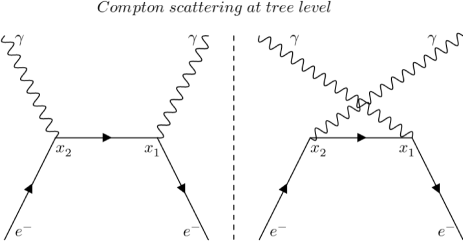
If we use the same notation and repeat for the present theory the same mathematical steps of Ref. man86 when it dealt with Compton scattering, we obtain that the part of the perturbative expansion of the S-matrix associated with the Feynman diagrams of Fig. 1 is
| (191) |
where in SI units we have
| (192) | |||||
| (193) | |||||
In Eqs. (192) and (193), and , where , are given by Eqs. (42)-(45), are the corresponding photon field expansions man86 , and is the fermion propagator given by Eq. (168).
If we look at Eqs. (42)-(45) and (168), we realize that the exponentials coming from , the exponentials coming from , and the exponential of are all canceled in Eqs. (192) and (193). As such, the mathematical steps leading to the transition matrix for Compton scattering are formally the same of standard QED. Therefore, following man86 we get
| (194) | |||||
| (195) | |||||
where, in an obvious notation and suppressing the spin and polarization indexes, , and
| (196) | |||||
| (197) |
In Eqs. (194) and (195), is given by Eq. (47) and is the corresponding normalization factor for the photon field expansion. In SI units,
| (198) |
where is the vacuum permeability and is defined in Eq. (142).
In Eqs. (196) and (197), is the Feynman propagator (176) in momentum space related to the Dirac-like equation (173) and is the photon’s polarization four-vector. In the Lorentz covariant quantization of the photon, there are four linearly independent polarization four-vectors.
If we use Eqs. (25), (181), (182), and (189), we immediately get
| (199) | |||||
| (200) |
Remembering that and are, respectively, the standard Dirac spinor and fermion propagator, we recognize Eqs. (199) and (200) as the Compton scattering Feynman amplitudes of standard QED man86 ; gre95 .
The previous example illustrates the general features present in any transition matrix and Feynman amplitude calculation within the theoretical framework of the asymmetric Dirac field QED. Point (A), with its corresponding map (189), will always be used to connect the asymmetric Dirac spinors with the standard ones and to connect the Feynman propagator from both theories. Point (B) allows us to express the conservation of energy and momentum directly in terms of the respective quantities for the asymmetric Dirac particles. For instance, in Eq. (194), we could have written , where and are, respectively, the energy and momentum for an asymmetric Dirac particle with wave number . The factor will always be canceled and therefore we can simply write the conservation of energy-momentum directly in terms of the corresponding quantities for the standard Dirac particles, according to the prescription given in point (B).
We should remark that this “cancellation” of the many ’s in the above four-dimensional Dirac delta function, as well as the cancellation of several exponential functions with exponents given by [see the discussion between Eqs. (193) and (194)], are ubiquitous and not a particular feature of the Compton scattering. These cancellations guarantee the validity of the crossing symmetry principle for the asymmetric Dirac field QED. In other words, whenever one can apply the crossing symmetry principle for the standard QED gre03 , one can also apply it to the asymmetric Dirac field QED.
Feynman rules in momentum space
The specific example above, as well as a general analysis similar to the ones in Refs. man86 ; gre95 , tells us that the Feynman rules in momentum space for the asymmetric Dirac field QED is the same as that for standard QED, with only one exception. Instead of the usual fermion propagator of QED in momentum space, we should use the propagator given by Eq. (176). Being more specific, whenever we have an internal fermion line labeled by the four-momentum , we should write the following factor,
| (201) |
The cross section
To finish the proof that both theories are empirically equivalent at the level of QED, we have to prove that the differential cross-sections derived from both theories for a given QED scattering process are the same. If we work through all the steps usually employed to build the differential cross section, we identify three major logical steps man86 ; gre95 . The first two, as summarized in Ref. rig22 , are easily seen to be the same for both theories due to points (A) and (B) given in Sec. VI.2. Indeed, the map of point (A) guarantees the equivalence of the transition probability per unit time and point (B) ensures that the conservation of energy and momentum applied to the asymmetric Dirac particles are properly mapped to the usual conservation of energy and momentum of standard Dirac particles. The last and third point man86 ; gre95 , as listed in Ref. rig22 , is:
-
•
The differential scattering cross section is generally defined as
(202) where , is the magnitude of the flux of incoming particles, and represents the number of final scattered particles having wave numbers between and . Here denotes the probability amplitude for a given process, is the duration of the experiment, and a finite box normalization is used for the incoming and outgoing particles wave functions such that we have one particle per volume .
Equation (202) leads to the same predictions for both theories if the flux of incoming particles computed within each theoretical framework is the same for a given wave number. The flux of particles is given by Eq. (23) if we drop the charge . If we use the plane wave solutions for the asymmetric Dirac equation as given in Sec. X of Ref. rig23 , a direct calculation gives
| (203) |
where . To obtain Eq. (203) we normalized such that , i.e., one particle per volume .
If we now compute for a standard Dirac particle, using the same previous normalization for its wave function, we also obtain Eq. (203). Moreover, for a standard relativistic particle we have in SI units gre00 ; man86 ; gre95 ,
| (204) |
Thus, Eq. (203) becomes
| (205) |
which defines the velocity of a particle within a beam of particles with a given wave number and flux .
Since we have just seen that in both theories the flux is the same, Eq. (205) implies that the asymmetric and standard Dirac particles have the same velocity . But for a standard relativistic particle, which implies that is also the velocity for an asymmetric Dirac particle sharing the same wave number with the corresponding standard Dirac particle. This is the justification of point (C) given in Sec. VI.2 and the proof that the differential cross section (202) are equivalent for both theories.
Note that the above differential cross section is the polarized one, where we have not summed or averaged over the fermion spins or photon polarizations. However, since Eq. (202) are equivalent in both theories, we can always first convert it to its standard QED analog and only then sum and average over all fermion spins and photons polarizations. This proves the equivalence of the unpolarized cross sections as well.
If we choose, nevertheless, to do all calculations directly using the asymmetric Dirac spinors, the computation of the unpolarized cross sections are slightly different since the “spin sums rules” man86 ; gre95 have to be adapted to the appropriate context. Of course, the final results will be the same, as the above discussion shows. We should also note that the “polarization sum rules” for the photons are easily seen to be the same of standard QED. This is true since the electromagnetic part of the asymmetric Dirac field QED are exactly the same of the standard one; we have adopted the same Lorentz covariant second quantization recipe for the photon field in both theories.
In order to show how to deal with the fermion spin sums directly using the asymmetric Dirac spinors, and without losing in generality, let us fix our attention on Compton scattering. The unpolarized cross-section for Compton scattering is proportional to man86
| (206) |
where is the Feynman amplitude for this process. The Feynman amplitude can be generically written as man86
| (207) |
where is an arbitrary matrix made of products of the usual gamma matrices.
Following man86 , we can write Eq. (206) as follows,
| (208) |
where
| (209) |
Note that in Eq. (208) we also sum over repeated spinor indexes.
So far, what is shown in Eq. (208) is formally the same to what we get when dealing with standard Dirac spinors. The difference shows up when we use Eq. (137), or Eq. (138) when we have instead of . Employing Eqs. (137) and (139) we get
| (210) |
If we now use Eq. (181) and the cyclic property of the trace, we can write Eq. (210) as follows,
| (211) |
Comparing Eq. (211) with the corresponding one for the standard QED man86 , we realize that the former can be obtained from the latter by the following substitutions,
| (212) |
Equation (211) together with three other similar ones, obtained by all different arrangements of the spinors and in Eq. (207), illustrate the general way of handling spin sums directly within the theoretical framework of the asymmetric Dirac field QED.
Incidentally, if we observe the computation of the unpolarized cross sections for the several QED processes as given in Ref. man86 , namely, lepton pair creation in electron-positron collisions, Bhabha scattering, Compton scattering where either we sum and average over the electron spins only or we sum and average over both the electron spins and photon polarizations, and the scattering of a fermion by an external electromagnetic field, we observe that is either or .
However, whenever is given by the product of an odd number of the gamma matrices and as, for instance, in the scattering processes listed above, a direct calculation gives
| (213) |
Equation (213) when inserted into Eq. (211) leads exactly to the corresponding expression for the standard QED. This is yet another way of seeing the equivalence of the unpolarized cross sections of the asymmetric Dirac field QED and the standard QED.
Moreover, since commutes with , we also have
| (214) |
which helps in proving the equivalence of Eq. (211) for both theories when we compute cross sections for electrons with particular helicity states man86 .
We should also mention that the equivalence between the standard QED and the asymmetric Dirac field QED goes beyond the tree level. Using Eqs. (182) and (189), and employing the prescriptions (A)-(C) of Sec. VI.2, we can map any Feynman amplitude and cross section from one theory to the corresponding ones of the other theory describing the same physical process. As such, higher order terms in perturbation theory describing a given scattering process, as well as the computation of the radiative corrections and the renormalization techniques from standard QED, can all be readily carried over to the asymmetric Dirac field QED, leading to the same results and predictions.
VII Beyond quantum electrodynamics
The arguments used in Sec. VI.2 to prove the equivalence between the standard and the asymmetric Dirac field QED can be straightforwardly carried over to analyze the possible equivalence of both theories when we employ a different type of interaction. Since the standard rules to compute the cross section for both theories are essentially the same if we adopt the prescriptions (A), (B), and (C) given in Sec. VI.2, the proof of the equivalence can be traced back to proving whether or not the interaction Hamiltonian density are equivalent in both theories.
As shown in Sec. VI, the interaction Hamiltonian density of QED, given by Eq. (187), is the same in both theories. This comes about because of the particular transformation rules connecting the fields of both theories, Eqs. (24) and (177), and because of the way responds to those transformation rules. Specifically, the first mathematical identity given by Eq. (181) is crucial to prove the equality of the interaction Hamiltonian in both theories. In other words, Eq. (187) is invariant under the action of Eqs. (24) and (177) because of Eq. (181).
Our first goal in this section is to investigate how the other Dirac bilinears respond to those transformation rules. As we will see, not all bilinears are invariant under the action of Eqs. (24) and (177). Our second goal is to investigate what kinds of interactions involving scalar and spinor fields, or different spinor fields, are allowed when we demand that the Lorentz symmetry be fully respected. We will see that the requirement for Lorentz invariant interactions restricts severely the types of interactions allowed for the asymmetric Dirac fields, a constraint that is stronger than the ones required for the standard Dirac fields. Finally, we will end this section investigating, in a very qualitative way, what might happen when we include interaction terms coming from massive and possibly non-abelian Gauge fields that transform under a proper Lorentz transformation similarly to the asymmetric Dirac fields. Again, the demand that we must have Lorentz invariant Hamiltonian densities leads to stringent constraints on the possible types of allowed interactions.
VII.1 Dirac bilinears
If we use Eqs. (24), (177), and (181), we readily obtain
| (215) | |||||
| (216) | |||||
| (217) | |||||
| (218) | |||||
| (219) | |||||
Here and is the completely antisymmetric four-dimensional Levi-Civita symbol, i.e., for and even permutations while for odd permutations.
Looking at Eqs. (215)-(219), we realize that only the bilinears given by Eqs. (217) and (218) have the same form when we go from the asymmetric Dirac fields to the standard ones. Equation (217) is the bilinear associated with QED, namely, the term proportional to the electric current that couples with the electromagnetic abelian gauge field describing the photon. The remaining three terms, Eqs. (215), (216), and (219), are mapped to different bilinears though.
For instance, an interaction term proportional to , with being an integer, will not lead to the same predictions if we work with the standard Dirac fields and an interaction term proportional to . Actually, according to Eq. (215), the predictions stemming from in the context of the asymmetric Dirac fields will be the same as those coming from in the context of the standard Dirac fields. Depending on the value of , an attractive interaction in the context of the asymmetric Dirac fields can be mapped to a repulsive one when we move to the standard Dirac fields. For example, when , is mapped to while when we have going to . The minus sign in the former case indicates a change in the sign of the coupling constant, a feature that is not seen in the latter case.
VII.2 More than one spinor field
We now assume, for definiteness, that we are dealing with two kinds of leptons. An electron and a different lepton, for instance, a muon or a tau. The asymmetric electron spinor will be denoted by while the other lepton spinor by . The corresponding standard Dirac spinors will be denoted by and , respectively.
Since different leptons have different masses, the asymmetric spinors and standard Dirac spinors are connected by [cf. Eqs. (24) and (177)],
| (220) | |||||
| (221) |
where stand for , an electron, or , the other lepton. Note that in the previous equations, and , with being either the mass of the electron or the mass of the other lepton [cf. Eqs. (5) and (6)].
For standard Dirac spinors, an interaction term proportional to
| (222) |
is perfectly legitimate. Here and in what follows the corresponding Hermitian conjugate term will be omitted for simplicity. And, as always, normal ordering is implicitly assumed. This interaction term is a Lorentz scalar under a proper Lorentz transformations since both and transform in exactly the same way after a proper Lorentz transformation gre00 ; man86 ; gre95 . Using the notation introduced in Sec. II, this means that
| (223) | |||||
| (224) |
where . Equations (223) and (224) when inserted into Eq. (222) clearly show that we have an interaction term respecting the Lorentz symmetry (invariant under a proper Lorentz transformation).
On the other hand, for the asymmetric Dirac spinors, an interaction proportional to
| (225) |
is not a Lorentz scalar under a proper Lorentz transformation since now and transform differently after it. This happens because the transformation rule for depends on the value of , as we realize looking at Eqs. (9)-(11), and each lepton has a different set of values for .
By making use of Eqs. (220) and (221), we can also understand why an interaction modeled by Eq. (225) violates the Lorentz symmetry. Inserting Eqs. (220) and (221) into Eq. (225) we get
| (226) |
The term at the right hand side of Eq. (226) is clearly an invariant under proper Lorentz transformations but is not since is not a four vector. This clearly shows that the Lorentz symmetry is broken for that type of interaction. Note that interactions given by , where only spinors of the same flavor are present, respect the Lorentz symmetry. In this case , which means that the Lorentz symmetry offending term is no longer present.
Therefore, we can only have an interaction involving different flavors and that respects the Lorentz symmetry if it is given by
| (227) |
where and are arbitrary positive integers.
VII.3 Complex scalar or gauge fields
Let us now investigate what types of interactions are allowed when, in addition to the two spinor fields above, we also have one complex scalar field. If we denote by a standard complex Klein-Gordon field, it is obvious that the following interaction term is Lorentz invariant,
| (228) |
where and are arbitrary positive integers. The analogous term involving the asymmetric fields, namely, the asymmetric Dirac spinors rig23 and the Lorentz covariant Schrödinger fields rig22 , is not in general a Lorentz invariant. The reason for this is related to the fact that these asymmetric fields have transformation rules under a proper Lorentz transformation that depend on the four invariants given by . This dependence shows up as a phase that is a function of the space-time variables and of . And since the invariants depend on the values of the rest masses associated with the interacting particles, in general the phases will not cancel out each other when we deal with particles having different masses.
Similarly to what we did in Sec. VII.2, we can understand the above point if we use Eqs. (220), (221), and the corresponding one connecting the Lorentz covariant Schrödinger fields with the standard complex Klein-Gordon ones rig22 ,
| (229) |
Here , with being the mass of the scalar particle described by .
If we use Eqs. (220), (221), and (229), the following interaction term in the context of the asymmetric fields can be written as
| (230) | |||||
The expression in the last line of Eq. (230) is clearly invariant under a proper Lorentz transformation. Thus, we can only make the whole expression invariant if
| (231) |
Equation (231) tells us that only certain combinations of the positive integers and may lead to a Lorentz invariant interaction. Indeed, each set of four invariants , with , is determined in such a way that it is compatible with the rest mass of the -th particle involved in the interaction above. With the values of fixed in this way, we have to choose and such that Eq. (231) is satisfied, guaranteeing an interaction that fully respects the Lorentz symmetry.
The argument above can be extended, or better yet, reversed, if instead of a scalar particle we have a massive complex gauge field (abelian or non-abelian) mediating the interaction between the two spinors. First, if it were possible to consistently develop a complex gauge field theory whose fields transform under a proper Lorentz transformation similarly to the asymmetric spinor and complex scalar fields studied here. Second, if we could consistently apply a “minimal coupling prescription” leading to the interaction between the asymmetric spinor and complex gauge fields, then a similar constraint given by Eq. (231), that guarantees the Lorentz invariance of the interaction (230), could be used to determine the mass of the gauge boson.
This would be the case because the interaction term would be fixed by the minimal coupling prescription. We no longer would be free to choose the interaction term. In other words, the values of and in the corresponding interaction term would not be arbitrary but determined by the specific form of the interaction arising after the minimal coupling prescription is applied. As such, we would have to choose the values of in order to satisfy a similar constraint as given by Eq. (231). And since the values of determine the mass of particle , the mass of the gauge boson would be fixed once the masses of the spinors enter as input. Note that theories built along these lines may also provide a fresh outlook in the understanding of the flavor puzzle fer15 .
Note that taking the previous argument at face value might lead to a electroweak theory that does not respect the lepton flavor universality gre00b . Indeed, to achieve universality all leptons should have the same coupling constant with a given boson and the interaction term should have the same functional form. Since we have three generations of leptons, we will run out of parameters to satisfy three similar expressions as given by Eq. (231). However, the electroweak theory is non-abelian and it is expected that for non-abelian gauge fields the phase of Eq. (229) will be generalized to a space-time dependent unitary matrix, whose dimension is related to the internal space dimension from which the non-abelian theory is built. This will eventually lead to more parameters than the ones appearing in the exponential of Eq. (230). As such, it is not unlikely that we may have enough parameters to determine the boson masses and, at the same time, keep lepton flavor universality. The definitive answer to this question can only be given when (and if) a non-abelian asymmetric field theory is fully developed.
VIII Conclusion
We showed that it is possible to consistently second quantize the asymmetric Dirac fields, which were introduced at the first quantization level in Ref. rig23 . By applying the electromagnetic minimal coupling prescription to the free field Lagrangian density describing the asymmetric Dirac fields, a fully renormalizable QED-like quantum field theory consistently emerged. Moreover, by properly choosing the parameters characterizing the free asymmetric spinorial fields, we proved that the obtained QED-like theory gives exactly the same predictions of the standard QED. This latter result is far from trivial and could not have been anticipated by simply inspecting the assumptions employed in the construction of the asymmetric scalar and Dirac fields rig22 ; rig23 .
Indeed, we can list the following four main features that set apart the present theory, and the corresponding scalar one given in Ref. rig22 , from the standard ones. First, the Lagrangian densities and the associated scalar and spinorial wave equations describing those asymmetric fields are formally different from the corresponding quantities related to the standard Klein-Gordon and Dirac fields. Second, the transformation rules for the asymmetric fields under a proper Lorentz transformation are fundamentally different from the rules for standard scalar and spinor fields. The asymmetric fields transformation rules, contrary to the standard ones, have a space-time dependent phase in addition to the usual rules. Third, the masses of the asymmetric particles are functions of four relativistic invariants that naturally appear in the free field Lagrangian densities. And these four relativistic invariants change sign after improper Lorentz transformations or after the charge conjugation operation in the same way as the components of a four-vector. The mass , though, is invariant under those same transformations since it depends quadratically on those invariants. Fourth, particles and antiparticles no longer have degenerate energies and momenta when sharing the same wave number. In its simplest formulation, we can build an asymmetric quantum field theory such that particles and antiparticles have the same momenta and a gap of in their energies while sharing the same wave number. Despite all these unusual features, the asymmetric classical and quantum field theories developed here and in Refs. rig22 ; rig23 respect the Lorentz symmetry and can be made equivalent to the standard Klein-Gordon and Dirac theories when minimally coupled to electromagnetic fields.
The next natural question is the extension of the present ideas, and those of Refs. rig22 ; rig23 , to massive gauge fields that transform under a proper Lorentz transformation similarly to the way the asymmetric scalar and Dirac fields do rig22 ; rig23 . In other words, can we build a renormalizable electroweak theory whose gauge fields but one (the photon field) are massive from the start, fully respects the Lorentz symmetry, and reproduces the predictions of the standard electroweak theory? Moreover, can we explore the asymmetry of the fields, namely, the gap in the energy between particles and antiparticles in order to provide a viable explanation for the asymmetry between matter and antimatter in our universe in a fully relativistic theory din04 ? Since antiparticles are more energetic than particles for a given wave number, it is not unlikely that a electroweak-like theory built on these principles may lead to antiparticles being more unstable than particles. And the CP violation, would it be stronger for those asymmetric fields? Would we get new sources of CP violation in this theoretical framework bra12 ; nis06 ; nis12 ; nis13 ; nis15 ? What about the strong force, can a theory describing it be formulated along the principles outlined here?
Another interesting question that deserves further exploration is related to the gravitational force. As qualitatively discussed here and in Refs. rig22 ; rig23 , the fact that the inertial mass of a particle, in the theoretical framework of the asymmetric fields, is a quadratic function of four relativistic invariants, suggests that the coupling of matter with the gravitational field can be implemented via those invariants instead of the mass itself. This opens the possibility to model the gravitational interaction between particles and antiparticles differently. It is possible to build a theory in which a particle and an antiparticle repel each other gravitationally while still keeping the masses and energies of particles and antiparticles positive rig22 ; rig23 . In this theory particles attract particles, antiparticles attract antiparticles, with the repulsive force only between a particle and an antiparticle rig22 ; rig23 . Would this approach to model the gravitational interaction lead to a consistent renormalizable quantum field theory of gravity? Would its predictions be consistent with the experimental data we have collected so far concerning the interaction of matter and antimatter with a gravitational field?
Finally, the ideas presented here and in Refs. rig22 ; rig23 show that it is possible to consistently build relativistic classical and quantum field theories whose scalar and spinorial fields transform in a non-standard way under proper Lorentz transformations. In spite of that, these theories can be made to reproduce exactly the experimental predictions of standard Klein-Gordon and Dirac fields interacting with photon fields, with the electromagnetic interaction being introduced via the minimal coupling prescription. Two other peculiar aspects of the asymmetric field theories developed here and Refs. rig22 ; rig23 lie in the non-degeneracy of the energy and momentum for a particle and antiparticle sharing the same wave number and the more stringent constraints on the possible types of interactions among those fields that fully respect the Lorentz symmetry. The non-degeneracy in the energy for particles and antiparticles does not lead to experimental predictions beyond the standard model at the level of QED, as we proved here. However, it is not unlikely that the formulation of a fundamental theory where flavor is not conserved (electroweak theory) in terms of asymmetric spinorial and gauge fields may lead to an experimental prediction beyond the standard model. In electroweak-like theories, the decay of particles is a fundamental aspect of those theories and the non-degeneracy in the energy of particles and antiparticles may manifest itself in different decay rates for particles and antiparticles sharing the same mass.
Acknowledgements.
The author thanks the Brazilian agency CNPq (National Council for Scientific and Technological Development) for partially funding this research.References
- (1) E. Schrödinger, An Undulatory Theory of The Mechanics of Atoms and Molecules, Phys. Rev. 28, 1049 (1926).
- (2) L. E. Ballentine, Quantum Mechanics: A Modern Development (World Scientific, Singapore, 1998).
- (3) W. Greiner, Relativistic Quantum Mechanics: Wave Equations (Springer-Verlag, Berlin, 2000).
- (4) G. Rigolin, On Lorentz Invariant Complex Scalar Fields, Adv. High Energy Phys 2022, 5511428 (2022).
- (5) G. Rigolin, Asymmetric particle-antiparticle Dirac equation: first quantization, arXiv:2205.04516.
- (6) P. A. M. Dirac, The Principles of Quantum Mechanics (Oxford University Press, London, 1967).
- (7) F. Mandl and G. Shaw, Quantum Field Theory (John Wiley & Sons, Chichester, 1986).
- (8) W. Greiner and J. Reinhardt, Field Quantization (Springer-Verlag, Berlin, 1996).
- (9) F. Schwabl, Advanced Quantum Mechanics (Springer-Verlag, Berlin, 2005).
- (10) N. N. Bogoliubov and D. V. Shirkov, Introduction to the Theory of Quantized Fields (John Wiley & Sons, New York, 1980).
- (11) V. I. Safonov, Conduction Electron in the Anisotropic Medium, Int. J. Mod. Phys. B 7, 3899 (1993).
- (12) A. Zhao, J. Zhang, Q. Gu, and R. A. Klemm, A relativistic electron in an anisotropic conduction band, arXiv:1905.03127.
- (13) M. S. Safronova, D. Budker, D. DeMille, D. F. J. Kimball, A. Derevianko, and C. W. Clark, Search for new physics with atoms and molecules, Rev. Mod. Phys. 90, 025008 (2018).
- (14) H. Bondi, Negative Mass in General Relativity, Rev. Mod. Phys. 29, 423 (1957).
- (15) M. Kowitt, Gravitational Repulsion and Dirac Antimatter, Int. J. Theor. Phys. 35, 605 (1996).
- (16) M. Villata, CPT symmetry and antimatter gravity in general relativity, EPL 94, 20001 (2011).
- (17) J. S. Farnes, A unifying theory of dark energy and dark matter: Negative masses and matter creation within a modified framework, A&A 620, A92 (2018).
- (18) W. Greiner and J. Reinhardt, Quantum Electrodynamics (Springer-Verlag, Berlin, 2003).
- (19) F. Feruglio, Pieces of the flavour puzzle, Eur. Phys. J. C 75, 373 (2015).
- (20) W. Greiner and B. Müller, Gauge Theory of Weak Interactions (Springer-Verlag, Berlin, 2000).
- (21) M. Dine and A. Kusenko, Origin of the matter-antimatter asymmetry, Rev. Mod. Phys. 76, 1 (2004).
- (22) G. C. Branco, R. González Felipe, and F. R. Joaquim, Leptonic CP violation, Rev. Mod. Phys. 84, 515 (2012).
- (23) C. C. Nishi, CP violation conditions in N-Higgs-doublet potentials, Phys. Rev. D 74, 036003 (2006).
- (24) R. N. Mohapatra and C. C. Nishi, flavored CP symmetry for neutrinos, Phys. Rev. D 86, 073007 (2012).
- (25) C. C. Nishi, Generalized CP symmetries in flavor models, Phys. Rev. D 88, 033010 (2013).
- (26) R. N. Mohapatra and C. C. Nishi, Implications of flavored CP symmetry of leptons, J. High Energ. Phys. 2015, 92 (2015).