Asymmetric Dark Matter abundance including non-thermal production

Maqingshan, Hoernisa Iminniyaz

School of Physics Science and Technology, Xinjiang University,
Urumqi 830046, China

1 Introduction

Dark Matter problem is undoubtedly one of the most challenging puzzles for cosmologists and particle physicists in recent years. Although we have most striking evidences for Dark Matter, the constitute of Dark Matter is still a mistery for us. Asymmetric Dark Matter is one alternatives which arises from the fact that its abundance is just 5 times larger than the baryon asymmetry [1]. There maybe an indication of common origin which is responsible for the baryonic asymmetry and Dark Matter. In asymmetric Dark Matter scheme, Dark Matter particle has its distinct antiparticle.

In standard cosmological scenario, it is supposed asymmetric Dark Matter were produced thermally. Based on the assumption that Weakly Interacting Massive Particles (WIMPs) constitute Dark Matter, the relic density of asymmetric Dark Matter is determined by the freeze-out condition [2, 3]. In this scenario, it is assumed the reheating temperature $T_{R}$ is much larger than the freeze out temperature $T_{F}$ and the asymmetric Dark Matter particles and anti–particles were in thermal equilibrium in the early universe. The final relic density of asymmetric Dark Matter mainly depends on the particle–antiparticle asymmetry and the indirect detection signals from annihilation is suppressed due to the reason that very little anti–particle is here in the end.

On the other hand, asymmetric Dark Matter can be produced non-thermally as heavy particles decay (e.g. moduli decay) into asymmetric Dark Matter. In ref.[4], the authors discussed a cogenesis mechanism in which the baryon asymmetry of the universe and Dark Matter abundance are simultaneously produced at low reheating temperature. Refs.[5] explored the non–thermal production of Dark Matter including asymmetric Dark Matter in the scheme of Minimal Supersymmetric Standard Model and string motivated models. Relic abundance of Dark Matter was calculated in ref.[6] including the decays of unstable heavy particle to Dark Matter particles. In our work, we investigate the relic density of asymmetric Dark Matter in low reheating temperature scenario when the heavy unstable particles $\phi$ decay into asymmetric Dark Matter particles and anti–particles. We suppose that the asymmetry is already existed before the decay of heavy particles into asymmetric Dark Matter and they decay into particle and anti–particle in the same amount. We still assume the universe is radiation dominated and the additional entropy production from the decay of heavy particle is negligible. The decay of heavier particles to asymmetric Dark Matter changes the total relic density of asymmetric Dark Matter. The relic abundances of asymmetric Dark Matter particle and anti–particle are both increased when there is additional contribution from the decay of heavier particles.

The outline of the paper is as following. In section 2, we discuss the relic density calculation of asymmetric Dark Matter including the decay of heavy particles into asymmetric Dark Matter in low temperature scenario. We find the approximate analytic solution for the relic density of asymmetric Dark Matter when there is thermal and non–thermal production. In section 3, the constraints on parameter spaces are obtained by using the Planck data. The last section is devoted to the brief summary and conclusions.

2 Relic abundance of asymmetric Dark Matter including non-thermal production

We discuss the scenario where the unstable heavy particles $\phi$ decay into asymmetric Dark Matter particles and anti–particles. Here we assume the heavy particle $\phi$ decays out of thermal equilibrium, therefore, $\phi$ production is negligible. However, we include the thermal and non–thermal production of asymmetric Dark Matter particles.

In the standard computation of relic density for the asymmetric Dark Matter, it was assumed the reheating temperature of the universe $T_{R}$ is much higher than the freeze out temperature. In this case, the reheating era has no effect on the final relic density of asymmetric Dark Matter. On the other hand, the constraints on the reheating temperature comes from Big Bang Nucleosynthesis and $T_{R}\raisebox{-3.69899pt}{~{}\shortstack{$>$ \\ [-0.07cm] $\sim$}}~{}1$ MeV [7, 8, 9]. Therefore, we consider the case where $T_{R}<T_{F}$ [10, 11, 12, 13]. The asymmetric Dark Matter particles and anti–particles never reach thermal equilibrium due to the low reheating temperature, we treat the asymmetric Dark Matter abundances at some initial temperature $T_{0}$ as a free parameter.

The evolution of relic abundance including the decay of heavy particles is more complicated than the usual thermal production case. Here we still assume the universe is radiation dominated and the entropy production is negligible. We suppose that asymmetry is existed before the decay of heavy particles and they decay into particle and anti–particle in the same amount. The coupled Boltzmann equations for the number densities $n_{\chi}$ and $n_{\bar{\chi}}$ of asymmetric Dark Matter particles $\chi$ and anti–particles $\bar{\chi}$ are as following,

$$\frac{dn_{\chi}}{dt}+3Hn_{\chi}=-\langle\sigma v\rangle(n_{\chi}n_{\bar{\chi}}-n_{\chi,{\rm eq}}n_{\bar{\chi},{\rm eq}})+N\Gamma_{\phi}n_{\phi},$$ (1)

$$\frac{dn_{\bar{\chi}}}{dt}+3Hn_{\bar{\chi}}=-\langle\sigma v\rangle(n_{\chi}n_{\bar{\chi}}-n_{\chi,{\rm eq}}n_{\bar{\chi},{\rm eq}})+N\Gamma_{\phi}n_{\phi},$$ (2)

$$\frac{dn_{\phi}}{dt}+3Hn_{\phi}=-\Gamma_{\phi}\,n_{\phi},$$ (3)

where $H$ is the expansion rate of the universe, and $\langle\sigma v\rangle$ is the thermal average of the cross section multiplied with the relative velocity of annihilating asymmetric Dark Matter particles and anti–particles. Here we assume only $\chi\bar{\chi}$ pairs can annihilate into Standard Model particles. $n_{\chi,{\rm eq}}$ is the equilibrium number density. $N$ is the average number of asymmetric Dark Matter particle and anti–particle produced in $\phi$ decay, $\Gamma_{\phi}$ is the decay rate. Here it is assumed that $\phi$ does not dominate the total energy density. Therefore, the comoving entropy density almost stays constant throughout. The analytic solution for Eq.(3) is easily obtained. Then Eqs.(1), (2) can be solved approximately in low temperature scenarios.

In order to simplify Eqs.(1),(2),(3), we introduce the following dimensionless variables $Y_{\chi,\bar{\chi}}=n_{\chi,\bar{\chi}}/s$, $Y_{\phi}=n_{\phi}/s$ and $x=m/T$ with $s$ being the entropy density, then

$$\frac{d(sY_{\chi})}{dt}+3HsY_{\chi}=-\langle\sigma v\rangle s^{2}(Y_{\chi}Y_{\bar{\chi}}-Y_{\chi,{\rm eq}}Y_{\bar{\chi},{\rm eq}})+N\Gamma_{\phi}\,sY_{\phi},$$ (4)

$$\frac{d(sY_{\bar{\chi}})}{dt}+3HsY_{\bar{\chi}}=-\langle\sigma v\rangle s^{2}(Y_{\chi}Y_{\bar{\chi}}-Y_{\chi,{\rm eq}}Y_{\bar{\chi},{\rm eq}})+N\Gamma_{\phi}\,sY_{\phi},$$ (5)

$$\frac{d(sY_{\phi})}{dt}+3HsY_{\phi}=-\Gamma_{\phi}\,sY_{\phi}\,,$$ (6)

Assuming entropy per comoving volume is conserved, we obtain

$$\dot{s}=-3sH,$$ (7)

here we used $H=\dot{R}/R$, where $R$ is the scale factor of the universe. Inserting $s=(2\pi^{2}/45)g_{*}T^{3}$ to Eq.(7), here $g_{*}$ is the effective number of relativistic degrees of freedom, we obtain

$$\frac{1}{T}\frac{dT}{dt}+\frac{1}{3g_{*}}\frac{dg_{*}}{dt}+H=0,$$ (8)

Using $T=m/x$

$$\frac{dx}{dt}=\frac{Hx}{1-\frac{x}{3g_{*}}\frac{dg_{*}}{dx}}\,.$$ (9)

Then Eqs.(4), (5) and (6) can be written as

$$\frac{dY_{\chi}}{dx}=-\frac{\langle\sigma v\rangle s}{Hx}(Y_{\chi}Y_{\bar{\chi}}-Y_{\chi,{\rm eq}}Y_{\bar{\chi},{\rm eq}})+\frac{N\Gamma_{\phi}}{Hx}Y_{\phi}\,,$$ (10)

$$\frac{dY_{\bar{\chi}}}{dx}=-\frac{\langle\sigma v\rangle s}{Hx}(Y_{\chi}Y_{\bar{\chi}}-Y_{\chi,{\rm eq}}Y_{\bar{\chi},{\rm eq}})+\frac{N\Gamma_{\phi}}{Hx}Y_{\phi}.$$ (11)

$$\frac{dY_{\phi}}{dx}=-\frac{\Gamma_{\phi}}{Hx}Y_{\phi},$$ (12)

here we assume $dg_{*}/dx=0$. Eq.(12) can be solved easily,

$$\int^{Y_{\phi}(x)}_{Y_{\phi}(x_{0})}\frac{dY_{\phi}}{Y_{\phi}}=-\int^{x}_{x_{0}}\frac{\Gamma_{\phi}dx}{Hx},$$ (13)

$$Y_{\phi}(x)=Y_{\phi}(x_{0})e^{-\int^{x}_{x_{0}}\frac{\Gamma_{\phi}dx}{Hx}}\,,$$ (14)

where $x_{0}$ is the inverse scaled initial temperature which is close to the freeze out temperature. Then equations (10) and (11) become

$$\frac{dY_{\chi}}{dx}=-\frac{\langle\sigma v\rangle s}{Hx}(Y_{\chi}Y_{\bar{\chi}}-Y_{\chi,{\rm eq}}Y_{\bar{\chi},{\rm eq}})+\frac{N\Gamma_{\phi}}{Hx}Y_{\phi}(x_{0})e^{-\int^{x}_{x_{0}}\frac{\Gamma_{\phi}}{Hx}\,dx}\,,$$ (15)

$$\frac{dY_{\bar{\chi}}}{dx}=-\frac{\langle\sigma v\rangle s}{Hx}(Y_{\chi}Y_{\bar{\chi}}-Y_{\chi,{\rm eq}}Y_{\bar{\chi},{\rm eq}})+\frac{N\Gamma_{\phi}}{Hx}Y_{\phi}(x_{0})e^{-\int^{x}_{x_{0}}\frac{\Gamma_{\phi}}{Hx}\,dx}\,.$$ (16)

In the radiation dominated era, $H=\pi m^{2}_{\chi}/(M_{\rm Pl}\,x^{2})\sqrt{g_{*}/90}$, where $m_{\chi}$ is the mass of asymmetric Dark Matter particle and $M_{\rm Pl}=2.4\times 10^{18}$ GeV is the reduced Planck mass. Now we further simplify Eqs.(15) and (16), subtracting equation (16) from equation (15), then

$$\frac{d(Y_{\chi}-Y_{\bar{\chi}})}{dx}=0.$$ (17)

This requires

$$Y_{\chi}-Y_{\bar{\chi}}=\eta.$$ (18)

Where $\eta$ is a constant. We can express equations (15) and (16) in terms of Eq.(18),

$$\frac{dY_{\chi}}{dx}=-\frac{\lambda_{1}\langle\sigma v\rangle}{x^{2}}\left(Y^{2}_{\chi}-\eta Y_{\chi}-\lambda_{2}x^{3}e^{-2x}\right)+\lambda_{3}NY_{\phi}(x_{0})x\,{\rm exp}\left[\frac{\lambda_{3}}{2}(x_{0}^{2}-x^{2})\right],$$ (19)

$$\frac{dY_{\bar{\chi}}}{dx}=-\frac{\lambda_{1}\langle\sigma v\rangle}{x^{2}}\left(Y^{2}_{\bar{\chi}}+\eta Y_{\bar{\chi}}-\lambda_{2}x^{3}e^{-2x}\right)+\lambda_{3}NY_{\phi}(x_{0})x\,{\rm exp}\left[\frac{\lambda_{3}}{2}(x_{0}^{2}-x^{2})\right],$$ (20)

where $\lambda_{1}=\frac{4\pi}{\sqrt{90}}m_{\chi}M_{\rm Pl}\sqrt{g_{*}}\,$, $\lambda_{2}=(0.145g_{\chi}/g_{*})^{2}$, and $\lambda_{3}=M_{\rm Pl}\Gamma_{\phi}/(\pi m^{2}_{\chi})\sqrt{90/g_{*}}$. Here we used the equilibrium abundance $Y_{\chi,\bar{\chi},{\rm eq}}=0.145g_{\chi}/g_{*}x^{3/2}{\rm e}^{-x(1\pm\mu_{\chi}/m)}\,$, where $\mu_{\chi}$ is the chemical potential for particle, $g_{\chi}$ is number of internal degrees of freedom. Usually the thermal average of $\sigma v$ is approximated by a nonrelativistic expansion:

$$\langle\sigma v\rangle=a+6\,bx^{-1}+{\cal O}(x^{-2})\,,$$ (21)

where $a$ is the $s$–wave contribution for the limit $v\to 0$ and $b$ is $p$–wave contribution for the suppressed $s$–wave annihilation.

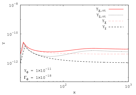
Figure 1: Evolution of $Y_{\chi}$ and $Y_{\bar{\chi}}$ as a function of $x$ for $Y_{\bar{\chi}}(x_{0}=22)=1\times 10^{-12}$, $N=1$ and $b=0$ $a=4\times 10^{-26}$ ${\rm cm}^{3}\,{\rm s}^{-1}$, $\eta=3\times 10^{-12}$, $m_{\chi}=100$ GeV, $x_{0}=22$, $g_{\chi}=2$, $g_{*}=90$. Here nt means non–thermal production.

Fig.1 depicts the evolution of relic abundances $Y_{\chi,\bar{\chi}}$ as a function of $x$ and it is based on the numerical solutions of Eqs.(19) and (20). Here solid red curve is for asymmetric Dark Matter particle abundance $Y_{\chi,{\rm nt}}$ with the decay of heavy particles and the black dotted curve is for antiparticle abundance $Y_{\bar{\chi},{\rm nt}}$. The red dot–dashed and black dashed curves are for asymmetric Dark Matter particle and anti–particle relic abundances $Y_{\chi}$ and $Y_{\bar{\chi}}$ without including the decay of heavy particles.

Fig.1 shows the abundances of asymmetric Dark Matter particle and anti–particle are increased because of the contribution from the decay of metastable heavier particles to asymmetric Dark Matter. The increase of the anti–particle abundance is more remarkable. We start from the initial value of $Y_{\bar{\chi}}(x_{0})$ at the initial temperature $x_{0}$. We assume asymmetric Dark Matter particles and anti–particles never reach thermal equilibrium because of the low reheating temperature. The particle and anti–particle abundances are increased quickly shortly after starting and then decreased both for thermal and non–thermal production. When $x$ increases, the abundances finally goes to constant value. The increases for particle and anti–particle abundances are slightly larger in panels $(b)$ and $(d)$ of Fig.1 for smaller decay rate with respect to panels $(a)$ and $(c)$. Comparing frames $(a)$ with $(c)$, and $(b)$ with $(d)$, we can see for lager initial value of $Y_{\phi}(x_{0})$, there is larger increases of the particle and anti–particle abundances. In frames $(c)$ and $(d)$, the anti–particle abundance almost catches the particle abundance finally. This opens the possibility to detect the asymmetric Dark Matter indirectly.

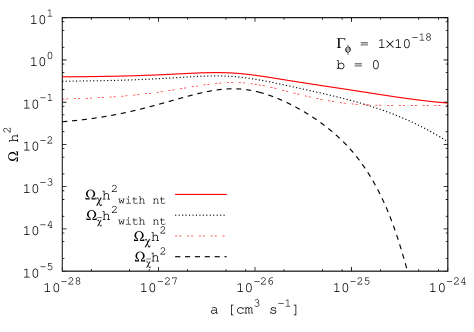
Figure 2: Relic density $\Omega h^{2}$ for particle $\chi$ and anti–particle $\bar{\chi}$ as a function of the $s-$wave cross section. Here $Y_{\bar{\chi}}(x_{0}=22)=1\times 10^{-12}$, $N=1$ and $Y_{\phi}=10^{-11}$, $\Gamma_{\phi}=10^{-18}$, $\eta=3\times 10^{-12}$, $m_{\chi}=100$GeV, $x_{0}=22$, $g_{\chi}=2$, $g_{*}=90$.

The changes of relic density $\Omega h^{2}$ as a function of the cross section is shown in Fig.2. It is for $s$–wave annihilation cross section with $b=0$ when asymmetry factor $\eta=3\times 10^{-12}$. Solid red curve and dotted black curve are for the relic densities of asymmetric Dark Matter particle and anti–particle with the decay of heavy particles. Double dotted red curve and black dashed curve are for the particle and anti–particle only with thermal production. Fig.2 shows when the cross sections increases, the depletion of anti–particle abundance is slower than the case of without including heavy particle decay.

Following we try to find the approximate analytical solutions of Eqs.(19) and (20). Eq.(20) can be solved first. At early times $(x<x_{0})$, $Y_{\bar{\chi},{\rm eq}}\gg Y_{\bar{\chi}}$, because usually $\eta$ is around $10^{-12}$ [3], $\eta Y_{\bar{\chi}}$ is small as well, therefore equation (20) becomes

$$\frac{dY_{\bar{\chi}}}{dx}=\lambda_{1}\lambda_{2}\langle\sigma v\rangle xe^{-2x}+\lambda_{3}NY_{\phi}(x_{0})x\,{\rm exp}\left(\frac{\lambda_{3}}{2}(x_{0}^{2}-x^{2})\right)\,.$$ (22)

Integrating above equation, we obtain

$$Y_{\bar{\chi}}(x) = {Y_{\bar{\chi}}(x_{0})}+\lambda_{1}\lambda_{2}\left[\frac{a}{2}(x_{0}\,e^{-2x_{0}}-x\,e^{-2x})+(\frac{a}{4}+3b)(e^{-2x_{0}}-e^{-2x})\right]$$ (23)

$$+ NY_{\phi}(x_{0})\,\left[1-{\rm exp}\left(\frac{\lambda_{3}}{2}(x_{0}^{2}-x^{2})\right)\right].$$

The abundance for $Y_{\chi}$ is obtained using Eq.(18),

$$Y_{\chi}(x) = \eta+{Y_{\bar{\chi}}(x_{0})}+\lambda_{1}\lambda_{2}\left[\frac{a}{2}(x_{0}\,e^{-2x_{0}}-x\,e^{-2x})+(\frac{a}{4}+3b)(e^{-2x_{0}}-e^{-2x})\right]$$ (24)

$$+ NY_{\phi}(x_{0})\,\left[1-{\rm exp}\left(\frac{\lambda_{3}}{2}(x_{0}^{2}-x^{2})\right)\right].$$

While the solution is valid only at early times, the relic abundances of particles and anti–particles are approximated for $x\gg x_{0}$ as,

$$Y_{\bar{\chi},\infty}\equiv Y_{\bar{\chi}}(x\gg x_{0})={Y_{\bar{\chi}}(x_{0})}+\lambda_{1}\lambda_{2}\left[\frac{a}{2}x_{0}\,e^{-2x_{0}}+(\frac{a}{4}+3b)e^{-2x_{0}}\right]+NY_{\phi}(x_{0}).$$ (25)

$$Y_{\chi,\infty}\equiv Y_{\chi}(x\gg x_{0})=\eta+{Y_{\bar{\chi}}(x_{0})}+\lambda_{1}\lambda_{2}\left[\frac{a}{2}x_{0}\,e^{-2x_{0}}+(\frac{a}{4}+3b)e^{-2x_{0}}\right]+NY_{\phi}(x_{0}).$$ (26)

The relative prediction for the present relic density is given by

$$\Omega_{\rm DM}h^{2}=\frac{\rho}{\rho_{c}}=2.76\times 10^{8}m_{\chi}[Y_{\chi,\infty}+Y_{\bar{\chi},\infty}]\,{\rm GeV}^{-1},$$ (27)

where the scaled Hubble constant $h$ in units of $100$ km s^-1 Mpc^-1 is $0.673\pm 0.098$. Here $\rho=nm=s_{0}Ym$ and the critic density is $\rho_{c}=3H^{2}_{0}M^{2}_{\rm Pl}$, where $s_{0}\simeq 2900$ cm^-3 is the present entropy density and $H_{0}$ is the Hubble constant.

In the late universe, for $x\gg x_{0}$,

$$Y_{\bar{\chi}}\gg Y_{\bar{\chi},{\rm eq}}.$$ (28)

Again the third and fourth terms in Eq.(20) decreases exponentially as $x$ increases, therefore, equation (20) becomes

$$\frac{dY_{\bar{\chi}}}{dx}=-\frac{\lambda_{1}\langle\sigma v\rangle}{x^{2}}\left(Y^{2}_{\bar{\chi}}+\eta Y_{\bar{\chi}}\right).$$ (29)

Integrating above equation, we obtain

$$Y_{\bar{\chi}}(x)=\frac{\eta}{\left[1+\eta/Y_{\bar{\chi}}(x_{0})\right]\,e^{\int^{x}_{x_{0}}\frac{\eta\lambda_{1}\langle\sigma v\rangle}{x^{2}}dx}-1}\,.$$ (30)

In the same way as Eq.(24), we have

$$Y_{\chi}(x)=\frac{\eta}{1-\left\{Y_{\bar{\chi}}(x_{0})/[\eta+Y_{\bar{\chi}}(x_{0})]\right\}\,e^{-\int^{x}_{x_{0}}\frac{\eta\lambda_{1}\langle\sigma v\rangle}{x^{2}}dx}}\,.$$ (31)

Inserting Eq.(21) into Eqs.(30) and (31), we obtain

$$Y_{\bar{\chi}}(x)=\frac{\eta}{\left[1+\eta/Y_{\bar{\chi}}(x_{0})\right]\,{\rm exp}\left\{\eta\lambda_{1}\left[a(1/x_{0}-1/x)+3b(1/x_{0}^{2}-1/x^{2})\right]\right\}-1}.$$ (32)

$$Y_{\chi}(x)=\frac{\eta}{1-\left\{Y_{\bar{\chi}}(x_{0})/[\eta+Y_{\bar{\chi}}(x_{0})]\right\}\,{\rm exp}\left\{\eta\lambda_{1}\left[a(1/x_{0}-1/x)+3b(1/x_{0}^{2}-1/x^{2})\right]\right\}}\,.$$ (33)

The final relic density is

$$\Omega_{\rm DM}h^{2}\simeq 2.76\times 10^{8}\,m\left[Y_{\chi}(x)+Y_{\bar{\chi}}(x)\right]\,.$$ (34)

3 Constraints on parameter space

The Planck team derived the Dark Matter relic density as [14],

$$\Omega_{\rm DM}h^{2}=0.1199\pm 0.0022\,.$$ (35)

We use the measured Dark Matter relic density to find constraints on the paramete space. For asymmetric Dark Matter, particle and anti–particle contributions have to be added as $\Omega_{\rm DM}=\Omega_{\chi}+\Omega_{\bar{\chi}}$.

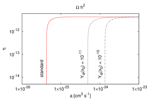
Figure 3: Contour plot of $s-$wave annihilation cross section $a$ and asymmetry factor $\eta$ when $\Omega_{\rm DM}h^{2}=0.1199$. The other parameters are the same as in Fig.2.

The contour plot of $s-$wave annihilation cross section and asymmetry factor $\eta$ is shown in Fig.3 when $\Omega_{\rm DM}h^{2}=0.1199$. This figure is based on the numerical solutions of the Bolzmann equations (19) and (20). The dotted (black) and dashed (black) curves are for the case of including the decay of heavier particle to asymmetric Dark Matter. The solid (red) curve is for the standard case. We find that the required cross section for $Y_{\phi}(x_{0})=10^{-11}$ is nearly one order of magnitude larger than the standard one in order to fall into the observational range. The increased relic density of asymmetric Dark Matter due to the decay of heavier particle is suppressed by the larger cross section. Furthermore, the figure shows that the needed cross section is slightly larger when the initial value of $Y_{\phi}$ is large. We note that the horizontal part of the contours is not affected by the decay of heavier particle. The anti–particle Dark Matter density of $Y_{\bar{\chi}}$ is exponentially suppressed when the asymmetry increases and the total Dark Matter relic density is determined by the particle density as $\Omega_{\rm DM}\sim mY_{\chi}\sim m\eta$. Therefore, the final relic density of DM is independent of the cross section $a$.

4 Summary and conclusions

The relic abundance of asymmetric Dark Matter including the decay of heavier particles is discussed in low reheating temperature scenario. Here we assume there is asymmetry before the unstable heavy particles decay into asymmetric Dark Matter particle and anti–particle in the same amount. We found that relic abundances of asymmetric Dark Matter particle and anti–particle are both increased when there is additional contribution from the decay of heavier particles. The increases of particle and anti–particle abundances due to the non–thermal production depends on the decay rate of heavy particles and slightly on the initial value of heavy particle abundance. Comparison with the usual thermal production shows that the depletion of the anti–particle abundance is slower for the case of including decay of heavy particles.

In the end, we used the observed DM abundance to obtain the constraints on the annihilation cross section and asymmetry factor when there is contribution from the decay of heavier particles to asymmetric Dark Matter. We found the required annihilation cross section with the decay of heavy particles is almost one order of magnitude larger than the case of without including non–thermal production. Those results are important for asymmetric Dark Matter. There is possibility to detect asymmetric Dark Matter in indirect detection due to the increased amount of anti–particle relic density when there is additional contribution from the decay of heavy particles.

References

- [1] S. Nussinov, Phys. Lett. B 165, (1985) 55; K. Griest and D. Seckel. Nucl. Phys. B 283, (1987) 681; R. S. Chivukula and T. P. Walker, Nucl. Phys. B 329, (1990) 445; D. B. Kaplan, Phys. Rev. Lett. 68, (1992) 742; D. Hooper, J. March-Russell and S. M. West, Phys. Lett. B 605, (2005) 228 [arXiv:hep-ph/0410114]; JCAP 0901 (2009) 043 [arXiv:0811.4153v1 [hep-ph]]; H. An, S. L. Chen, R. N. Mohapatra and Y. Zhang, JHEP 1003, (2010) 124 [arXiv:0911.4463 [hep-ph]]; T. Cohen and K. M. Zurek, Phys. Rev. Lett. 104, (2010) 101301 [arXiv:0909.2035 [hep-ph]]. D. E. Kaplan, M. A. Luty and K. M. Zurek, Phys. Rev. D 79, (2009) 115016 [arXiv:0901.4117 [hep-ph]]; T. Cohen, D. J. Phalen, A. Pierce and K. M. Zurek, Phys. Rev. D 82, (2010) 056001 [arXiv:1005.1655 [hep-ph]]; J. Shelton and K. M. Zurek, Phys. Rev. D 82, (2010) 123512 [arXiv:1008.1997 [hep-ph]];
- [2] M. L. Graesser, I. M. Shoemaker and L. Vecchi, JHEP 1110, (2011) 110 [arXiv:1103.2771 [hep-ph]].
- [3] H. Iminniyaz, M. Drees and X. Chen, “Relic Abundance of Asymmetric Dark Matter,” JCAP 1107, (2011) 003 [arXiv:1104.5548 [hep-ph]].
- [4] M. Dhuria, C. Hati and U. Sarkar, Phys. Lett. B 756 (2016), 376-383 doi:10.1016/j.physletb.2016.03.018 [arXiv:1508.04144 [hep-ph]].
- [5] N. Blinov, J. Kozaczuk, A. Menon and D. E. Morrissey, Phys. Rev. D 91 (2015) no.3, 035026 doi:10.1103/PhysRevD.91.035026 [arXiv:1409.1222 [hep-ph]].
- [6] M. Drees, H. Iminniyaz and M. Kakizaki, Phys. Rev. D 73 (2006), 123502 doi:10.1103/PhysRevD.73.123502 [arXiv:hep-ph/0603165 [hep-ph]].
- [7] G. F. Giudice, E. W. Kolb and A. Riotto, Phys. Rev. D 64 (2001), 023508 doi:10.1103/PhysRevD.64.023508 [arXiv:hep-ph/0005123 [hep-ph]].
- [8] S. Hannestad, Phys. Rev. D 70 (2004), 043506 doi:10.1103/PhysRevD.70.043506 [arXiv:astro-ph/0403291 [astro-ph]].
- [9] K. Ichikawa, M. Kawasaki and F. Takahashi, Phys. Rev. D 72 (2005), 043522 doi:10.1103/PhysRevD.72.043522 [arXiv:astro-ph/0505395 [astro-ph]].
- [10] N. Fornengo, A. Riotto and S. Scopel, Phys. Rev. D 67 (2003), 023514 doi:10.1103/PhysRevD.67.023514 [arXiv:hep-ph/0208072 [hep-ph]].
- [11] M. Bastero-Gil and S. F. King, Phys. Rev. D 63 (2001), 123509 doi:10.1103/PhysRevD.63.123509 [arXiv:hep-ph/0011385 [hep-ph]].
- [12] A. Kudo and M. Yamaguchi, Phys. Lett. B 516 (2001), 151-155 doi:10.1016/S0370-2693(01)00938-8 [arXiv:hep-ph/0103272 [hep-ph]].
- [13] G. B. Gelmini and P. Gondolo, Phys. Rev. D 74 (2006), 023510 doi:10.1103/PhysRevD.74.023510 [arXiv:hep-ph/0602230 [hep-ph]].
- [14] P. A. R. Ade et al. [Planck Collaboration], “Planck 2015 results. XIII. Cosmological parameters,” Astron. Astrophys. 594, (2016) A13 [arXiv:1502.01589 [astro-ph.CO]].