Calibrated Selective Classification

Abstract

Selective classification allows models to abstain from making predictions (e.g., say “I don’t know”) when in doubt in order to obtain better effective accuracy. While typical selective models can be effective at producing more accurate predictions on average, they may still allow for wrong predictions that have high confidence, or skip correct predictions that have low confidence. Providing calibrated uncertainty estimates alongside predictions—probabilities that correspond to true frequencies—can be as important as having predictions that are simply accurate on average. However, uncertainty estimates can be unreliable for certain inputs. In this paper, we develop a new approach to selective classification in which we propose a method for rejecting examples with “uncertain” uncertainties. By doing so, we aim to make predictions with well-calibrated uncertainty estimates over the distribution of accepted examples, a property we call selective calibration. We present a framework for learning selectively calibrated models, where a separate selector network is trained to improve the selective calibration error of a given base model. In particular, our work focuses on achieving robust calibration, where the model is intentionally designed to be tested on out-of-domain data. We achieve this through a training strategy inspired by distributionally robust optimization, in which we apply simulated input perturbations to the known, in-domain training data. We demonstrate the empirical effectiveness of our approach on multiple image classification and lung cancer risk assessment tasks.

1 Introduction

Even the best machine learning models can make errors during deployment. This is especially true when there are shifts in training and testing distributions, which we can expect to happen in nearly any practical scenario Quionero-Candela et al. (2009); Rabanser et al. (2019); Koh et al. (2021). Selective classification is an approach to mitigating the negative consequences of potentially wrong predictions, by allowing models to abstain on uncertain inputs in order to achieve better accuracy Chow (1957); El-Yaniv & Wiener (2010); Geifman & El-Yaniv (2017). While such systems may indeed be more accurate on average, they still fail to answer a critical question: how reliable are the uncertainties that they use to base their predictions? Often it can be important to precisely quantify the uncertainty in each prediction via calibrated confidence metrics (that reflect the true probability of an event of interest, such as our model being correct). This is particularly relevant in situations in which a user cannot easily reason about themselves in order to verify predictions; in which there is inherent randomness, and accurate predictions may be impossible; or in which high-stakes decisions are made, that require weighing risks of alternative possible outcomes Amodei et al. (2016); Jiang et al. (2018); Ovadia et al. (2019).

Consider the task of lung cancer risk assessment, where a model is asked if a patient will develop cancer within the next few years Aberle et al. (2011). A standard selective classifier may only make predictions on examples with clear outcomes; predictions that are less useful to the radiologists who these models are meant to help Dromain et al. (2013); Choy et al. (2018). Furthermore, even if the selective classifier is accurate, it may fail to accurately reflect the risk variations of different patients. For example, suppose that a patient has a 30% chance of developing cancer in reality. The prediction that the patient will not develop cancer will most likely be correct. However, knowing the degree of uncertainty in this outcome—namely that the patient’s true risk of developing cancer is 30%—might dramatically change the patient’s care plan. For these reasons, having a calibrated confidence estimate (in this case, that reflects the true likelihood of developing cancer) can be key to guiding clinical decision making Jiang et al. (2012); Tsoukalas et al. (2015).

We develop a new approach to selective classification in which we aim to only make predictions with well-calibrated uncertainties. In our lung cancer setting, this means that if the model predicts a cancer to develop with confidence $\alpha$ for a group of patients, then a fraction $\alpha$ of them should indeed develop cancer. Under our framework, a model should abstain if it is uncertain about its confidence, rather than risk misleading a user. In other words, we shift the focus from abstaining on uncertain examples, to abstaining on examples with “uncertain” uncertainties. Figure 1 illustrates our approach.

Figure 1: A demonstration of calibrated selective classification for lung cancer risk assessment. The input $X$ is a CT scan; the output $Y$ denotes if the patient develops cancer within 6 years of the scan ($Y=1)$, or not ($Y=0$). $f$ (yellow) provides a confidence estimate for the patient being at risk for cancer, while $g$ (red) acts as a gatekeeper to decide when to use $f$’s predictions. Our goal is for the accepted predictions to be calibrated. For example, over a population of patients with predicted (and non-rejected) risks of $0.7$, 70% should be expected to develop cancer within 6 years of the scan.

Concretely, consider a binary classification task (we consider multi-class tasks later) with input space $\mathcal{X}$ and label space $\mathcal{Y}=\{0,1\}$, where inputs $X\in\mathcal{X}$ and labels $Y\in\mathcal{Y}$ are random variables drawn from a joint distribution $P$. Suppose we have a model $f:\mathcal{X}\rightarrow[0,1]$, where $f(X)$ represents the model’s confidence that $Y=1$, while $1-f(X)$ represents the confidence that $Y=0$. Following the selective classification setting of Geifman & El-Yaniv (2017), we assume that $f$ is fixed (e.g., it may be a black-box or expensive to re-train)—and we are now simply seeking a safe gate-keeping mechanism for its predictions. Typical calibration stipulates that $\forall\alpha$ in the range of $f$, $\mathbb{E}[Y\mid f(X)=\alpha]=\alpha$ —but this may not be satisfied by the provided $f$. Instead, here we let $g\colon\mathcal{X}\rightarrow\{0,1\}$ be our selection model, where we make a prediction if $g(X)=1$, and abstain otherwise. Our goal is to make predictions that are calibrated conditioned on $g(X)=1$,

$$\mathbb{E}\big{[}Y\mid f(X)=\alpha,~{}g(X)=1\big{]}=\alpha,\hskip 15.0pt\forall\alpha\in[0,1]\text{ in the range of $f$ restricted to $\{x:g(x)=1\}$}.$$ (1)

We refer to this property as selective calibration. In practice, it is also important for $g$ to preserve some minimum amount of prediction coverage for $f$ to still be useful (e.g., we may want to make predictions on at least 80% of inputs). As a result, we seek to become as relatively calibrated as possible by minimizing the selective calibration error of $(f,g)$, i.e., deviation from Eq. (1), subject to a coverage constraint on $g$ that the user specifies. Inspired by the trainable Maximum Mean Calibration Error (MMCE) proxy objective of Kumar et al. (2018), we propose the Selective Maximum Mean Calibration Error (S-MMCE), that we train $g$ with to improve the selective calibration error.

Without knowing the test distribution, $P=P_{\mathrm{test}}$, that we will encounter, it is difficult to train $g$ to improve the selective calibration error on it. To address this, we formulate a robust calibration objective using synthetically constructed dataset shifts. Specifically, given some original training data $\mathcal{D}_{\mathrm{train}}\sim P_{\mathrm{train}}$ that we do have, and some family $\mathcal{T}$ of perturbations that we can define (e.g., via common data augmentation techniques), we minimize the S-MMCE over the uncalibrated datasets that we create by applying perturbations in $\mathcal{T}$ to the data in $\mathcal{D}_{\mathrm{train}}$. Of course, we do not expect these augmentations to represent all possible test distributions $P_{\mathrm{test}}$. Rather, by constructing a broad, albeit still limited, set of example shifts, our intention is for $g$ to learn to generalize well to new perturbation types, beyond those seen during training. Still, this is not guaranteed, and naturally, $g$’s generalization abilities will depend on how feasible it is to create a meaningful perturbation family $\mathcal{T}$. Empirically, however, when training and testing on disjoint sets of both simulated and naturally occurring perturbations on diverse datasets, we demonstrate consistent empirical reductions in selective calibration error metrics relative to typical confidence-based baselines across multiple tasks and datasets.

Contributions. To summarize, the main contributions of this work are as follows:

1. We introduce the concept of selective calibration, as an alternative to the typical selective classification objective;

2. We propose a coverage-constrained objective (S-MMCE) for training selectors to identify well-calibrated predictions;

3. We provide a robust framework for training calibration-seeking selectors that generalize to out-of-distribution data;

4. We demonstrate consistent empirical reductions in selective calibration error metrics (e.g., 18-25% reduction in $\ell_{2}$ calibration error AUC) relative to typical heuristic baselines (e.g., confidence-based) across multiple tasks and datasets.

2 Related work

Selective classification.  Selective classification, or classification with a reject option, attempts to abstain on examples that the model is likely to get wrong El-Yaniv & Wiener (2010); Geifman & El-Yaniv (2017). The literature on selective classification is extensive Hellman (1970); De Stefano et al. (2000); Herbei & Wegkamp (2006); Cortes et al. (2016a; b); Geifman & El-Yaniv (2019). A straightforward and popular technique is to use some confidence measure to select the most certain examples Cordella et al. (1995); El-Yaniv & Wiener (2010); Wiener & El-Yaniv (2012); Geifman & El-Yaniv (2017). If the underlying confidence measure is unreliable this approach can perform poorly Jones et al. (2021). As in our setting, Kamath et al. (2020) consider selective classification in the context of domain shift, though they focus on accuracy, rather than calibration. Approaches to selective classification that build beyond simple accuracy include cost-sensitive selective classification Bartlett & Wegkamp (2008); Charoenphakdee et al. (2021), selective classification optimized for experts in-the-loop Mozannar & Sontag (2020), and selective classification with fairness constraints Shah et al. (2021); all of which represent complementary directions to our work. Here, we extend selective classification to focus on improving model calibration over non-rejected instances.

Model calibration.  Calibration has a rich history in machine learning Brier (1950); Murphy & Epstein (1967); Dawid (1982); Foster & Vohra (1998); Gneiting et al. (2007). Recently, it has begun to experience a resurgence in the deep learning literature Kuleshov & Liang (2015); Kuleshov et al. (2018); Kumar et al. (2019); van Amersfoort et al. (2020); Gupta et al. (2020); Bates et al. (2020); Angelopoulos et al. (2022), partly motivated by observations that modern neural networks can be significantly miscalibrated out-of-the-box Guo et al. (2017b); Ashukha et al. (2020). To start, a number of efforts have focused on how to best define and measure calibration, especially in multi-class settings. A common approach (e.g., as taken by Guo et al. (2017a)) measures the top-label calibration error, or the probability that the model’s top prediction is correct (a definition we adopt). Other methods propose more precise notions of calibration, including calibration that is conditioned on the predicted class Gupta & Ramdas (2022), across classes Kull et al. (2019), for sub-populations or individuals Hebert-Johnson et al. (2018); Zhao et al. (2020), or tailored towards decision making Zhao et al. (2021). We note that these methods are complementary to our work, and could be incorporated in a selective setting following our framework. Approaches to actually achieving better calibration include both parameteric and non-parametric post-processing techniques Platt (1999); Zadrozny & Elkan (2001); Niculescu-Mizil & Caruana (2005); Guo et al. (2017a); Kumar et al. (2019), as well as modified losses introduced during model training Kumar et al. (2018); Mukhoti et al. (2020); Karandikar et al. (2021). Here, we attempt to achieve better conditional calibration across domains through selective classification.

Robustness to domain shift.  It is well-known that model performance can often degrade when the testing and training distributions are different—and many methods have been proposed to help combat this poor behavior Sugiyama & Müller (2005); Wen et al. (2014); Reddi et al. (2015); Lipton et al. (2018); Tran et al. (2022). With respect to model calibration, even models that are well-calibrated in-domain can still suffer from considerable miscalibration under domain shift Ovadia et al. (2019); Minderer et al. (2021). Given some knowledge or assumptions about the possible new target distribution (e.g., such as an estimated likelihood ratios or maximum divergence) several works have considered corrections for calibration under distribution shift Tibshirani et al. (2019); Cauchois et al. (2020); Gupta et al. (2020); Park et al. (2022). Similarly, given samples from two distributions (e.g., the training and testing distributions), many tests exist for detecting if they are different Vovk et al. (2003); Gretton et al. (2012); Chwialkowski et al. (2015). A shift in input features, however, is neither necessary nor sufficient as a predictor of accuracy; methods such as Ginart et al. (2022) attempt to monitor when distribution drifts are severe enough to indeed cause a performance drop, in order to trigger a decision to collect more supervised data. Closer to our work, a number of approaches have also attempted robust training (e.g., for temperature scaling) over multiple environments or domains Wald et al. (2021); Yu et al. (2022), rather than relying on test-time adjustments. Our work adds to the broad array of tools in this area by providing a general selective classification mechanism with few assumptions or requirements, that is specifically designed with domain shift in mind.

Synthetic perturbations.  Data augmentation is commonly used to improve model performance and generalization Hendrycks et al. (2020); Rusak et al. (2020); Cubuk et al. (2020); Buslaev et al. (2020). Similarly, automated methods have been developed for identifying challenging sub-populations of a larger training set to target bias Liu et al. (2021); Bao & Barzilay (2022). Meanwhile, we create perturbed datasets by sampling different augmentation types, in order to uncover relationships between types of perturbations and model calibration. These two lines of work are complementary: as new approaches are developed to expand the space of possible perturbations, the more tools our framework has to use.

3 Background

We begin with a brief review of selective classification and calibration. Throughout the paper, upper-case letters ($X$) denote random variables; lower-case letters ($x$) denote scalars; and script letters ($\mathcal{X}$) denote sets, unless otherwise specified.

3.1 Selective classification

Returning to the setting in §1, let $f\colon\mathcal{X}\rightarrow\mathcal{Y}$ be our prediction model with input space $\mathcal{X}$ and label space $\mathcal{Y}$, and let $g\colon\mathcal{X}\rightarrow\{0,1\}$ be a binary selection function over the input space $\mathcal{X}$. Let $P$ be a joint distribution over $\mathcal{X}\times\mathcal{Y}$. For now, we make no distinction between $P_{\mathrm{train}}$ and $P_{\mathrm{test}}$, and simply assume a general $P=P_{\mathrm{train}}=P_{\mathrm{test}}$. A selective classification system $(f,g)(x)$ at an input $x\in\mathcal{X}$ can then be described by the prediction rule

$$(f,g)(x):=\left\{\begin{array}[]{@{}l@{\thinspace}l}~{}f(x)&\hskip 17.07164pt\text{if }g(x)=1,\\[5.0pt] ~{}\text{``abstain''}&\hskip 17.07164pt\text{otherwise.}\end{array}\right.$$ (2)

Selective classifier performance is commonly evaluated in terms of risk versus coverage El-Yaniv & Wiener (2010). Coverage is defined as the probability mass of the region of $\mathcal{X}$ that is not rejected, $\psi(f,g;P):=\mathbb{E}[g(X)]$. In practice, $\psi(f,g;P)$ is usually tunable via a threshold $\tau\in\mathbb{R}$, where given some soft scoring function $\tilde{g}\colon\mathcal{X}\rightarrow\mathbb{R}$, $g$ is defined as $g(x):=\mathbf{1}\{\tilde{g}(x)\geq\tau\}$. Given some loss function $\mathcal{L}$, the selective risk with respect to $P$ is then defined as

$$\mathcal{R}(f,g;P):=\mathbb{E}[\mathcal{L}(f(X),Y)\mid g(X)=1]=\frac{\mathbb{E}[\mathcal{L}(f(X),Y)g(X)]}{\psi(f,g;P)}.$$ (3)

$\mathcal{L}$ is typically the $0/1$ loss, making $\mathcal{R}(f,g;P)$ the selective error. As evident from Eq. (3), there is a strong dependency between risk and coverage. Tuning $g$ to reject more examples can result in lower selective risk, but also lower coverage. The risk-coverage curve, $\mathcal{R}(f,g;P)$ plotted at different $\psi(f,g;P)$, and its AUC provide a standard way to evaluate and compare models. In this work we use will use AUC to evaluate the calibration-coverage curve of our proposed method.

3.2 Model calibration

We consider two simple marginal measures of calibration error, defined for both binary and multi-class classifiers. Starting with the binary setting, let $f\colon\mathcal{X}\rightarrow[0,1]$ be our model, where $f(X)$ is the confidence that $Y=1$. The binary calibration error measures the expected difference between $f(X)$, and the true probability of $Y$ given that estimate.

Definition 3.1 (Binary calibration error).

The $\ell_{q}$ binary calibration error of $f$ w.r.t. $P$ is given by

$$\mathrm{BCE}(f;q,P):=\big{(}\mathbb{E}\big{[}|\mathbb{E}[Y\mid f(X)]-f(X)|^{q}\big{]}\big{)}^{\frac{1}{q}}$$ (4)

Typical choices for the parameter $q\geq 1$ are $1$, $2$, and $\infty$ Murphy & Epstein (1967); Gneiting et al. (2007); Guo et al. (2017a); Kumar et al. (2019); Nixon et al. (2019); Gupta et al. (2020). We will use both $q=2$ and $q=\infty$ in this work.

We now turn to the multi-class case, where $\mathcal{Y}=\{1,\ldots,K\}$ is a finite label set with $K$ classes, and the model $f\colon\mathcal{X}\rightarrow[0,1]^{K}$ outputs a confidence score for each of the $K$ classes in $\mathcal{Y}$. A common measure of calibration is to take the difference between the model’s highest confidence in any one class, $\max_{y\in[K]}f(X)_{y}$, and the probability that the top predicted class, $\operatorname*{arg\,max}_{y\in[K]}f(X)_{y}$, is correct given that estimate Guo et al. (2017a); Kumar et al. (2019):

Definition 3.2 (Top-label calibration error).

The $\ell_{q}$ top-label calibration error of $f$ w.r.t. $P$ is given by

$$\mathrm{TCE}(f;q,P):=\big{(}\mathbb{E}\big{[}|\mathbb{E}[\mathbf{1}\{Y=\underset{{y\in[K]}}{\operatorname*{arg\,max}}~{}f(X)_{y}\}\mid\underset{y\in[K]}{\vphantom{\operatorname*{arg\,max}}\max}~{}f(X)_{y}]-\underset{y\in[K]}{\vphantom{\operatorname*{arg\,max}}\max}~{}f(X)_{y}|^{q}\big{]}\big{)}^{\frac{1}{q}}$$ (5)

In practice, we measure the empirical calibration error, where $\mathrm{BCE}$ and $\mathrm{TCE}$ are approximated with finite samples—see Appendix A for details. Having zero calibration error (according to the definitions above), however, does not imply that $f$ is a useful model. It is still important for $f$ to be a good predictor of $Y$. For example, the estimator $f(X):=\mathbb{E}[Y]$ is calibrated, but not necessarily accurate. As another measure of quality, we also report the Brier score Brier (1950):

Definition 3.3 (Brier score).

The mean-squared error (a.k.a., Brier score) of $f$ w.r.t. $P$ is given by

$$\mathrm{Brier}(f;P):=\mathbb{E}[(f(X)-Y)^{2}]$$ (6)

In multi-class scenarios, we set $f(X)$ and $Y$ to $\max_{y\in[K]}f(X)_{y}$ and $\mathbf{1}\{Y=\operatorname*{arg\,max}_{y\in[K]}f(X)_{y}\}$, respectively. Note that the Brier score and calibration error are related—it can be shown that the Brier score decomposes into the sum of the squared $\ell_{2}$ calibration error and an additional “sharpness” term Murphy (1973); DeGroot & Fienberg (1983).

4 Calibrated selective classification

We now propose an approach to defining—and optimizing—a robust selective calibration objective. In particular, we pursue an answer to the following high-level, motivating question:

Can we selectively classify examples such that the calibration of our model is improved on non-rejected instances?

We begin with a definition of selective calibration for selective classification (§4.1), as initially proposed in §1. We then present a trainable objective for selective calibration (§4.2), together with a coverage constraint (§4.3). Finally, we construct a robust framework for training calibrated selective classifiers that may encounter domain shift at test time (§4.4). For notational convenience, we focus our discussion on binary classification, but evaluate on both binary and multi-class selective classification tasks in our experiments. As stated in §1, we assume that $f$ is a pre-trained and fixed black-box that is only used to supply predictions—and we only train $g$. We leave joint training of the model $f$ and selector $g$ (e.g., following Geifman & El-Yaniv (2019)) to future work. We defer all proofs to Appendix LABEL:app:proofs.

4.1 Selective calibration

Once more, let $\mathcal{X}$ be our input space and $\mathcal{Y}=\{0,1\}$ be our binary label space with joint distribution $P$. Again, we assume for now that P is known and fixed (i.e., $P=P_{\mathrm{train}}=P_{\mathrm{test}}$). As introduced in §1, when classification model $f:\mathcal{X}\rightarrow[0,1]$ is paired with a selection model $g\colon\mathcal{X}\rightarrow\{0,1\}$, we can define selective calibration as follows:

Definition 4.1 (Selective calibration).

A binary selective classifier $(f,g)$ is selectively calibrated w.r.t. $P$ if

$$\mathbb{E}\big{[}Y\mid f(X)=\alpha,~{}g(X)=1\big{]}=\alpha,\hskip 15.0pt\forall\alpha\in[0,1]\text{ in the range of $f$ restricted to $\{x:g(x)=1\}$}.$$ (7)

Similarly, we also define the selective calibration error, which measures deviation from selective calibration.

Definition 4.2 (Selective calibration error).

The $\ell_{q}$ binary selective calibration error of $(f,g)$ w.r.t $P$ is

$$\mathrm{S\text{-}BCE}(f,g;q,P):=\Big{(}\mathbb{E}\Big{[}\big{|}\mathbb{E}[Y\mid f(X),~{}g(X)=1]-f(X)\big{|}^{q}\mid g(X)=1\Big{]}\Big{)}^{\frac{1}{q}}.$$ (8)

The top-label selective calibration error for multi-class classification is defined analogously, as is the selective Brier score. What might we stand to gain by using $(f,g)$ selectively? As a basic observation, we show that the coverage-constrained selective calibration error of $(f,g)$ can, in theory, always improve over its non-selective counterpart.

Claim 4.3 (Existence of a good selector).

For any fixed $f\colon\mathcal{X}\rightarrow[0,1]$, distribution $P$, and coverage level $\xi\in(0,1]$, there exists some (non-trivial) $g\colon\mathcal{X}\rightarrow\{0,1\}$ such that (i) $\mathbb{E}[g(X)]\geq\xi$, and (ii) $\mathrm{S\text{-}BCE}(f,g;q,P)\leq\mathrm{BCE}(f;q,P)$.

To provide some intuition on when an effective selection rule may be applied, consider the following toy setting.

Example 4.4 (Toy setting).

Assume that two-dimensional input $X=(X_{1},X_{2})\in[0,1]\times\{0,1\}$ follows the distribution $P_{X}:=\mathrm{Unif}(0,1)\times\mathrm{Bern}(\xi)$ for some $\xi\in(0,1)$, and output $Y\in\{0,1\}$ follows the conditional distribution

$$P_{Y\mid X}:=\left\{\begin{array}[]{@{}l@{\thinspace}l}~{}\mathrm{Bern}(X_{1})&\hskip 17.07164pt\text{if }X_{2}=1,\\[5.0pt] ~{}\mathrm{Bern}(\min(X_{1}+\Delta,1))&\hskip 17.07164pt\text{if }X_{2}=0,\end{array}\right.$$ (9)

for some $\Delta>0$. The confidence predictor (given to us) is simply $f(X)=X_{1}$. That is, by design, $f(X)\mid X_{2}=1$ is perfectly calibrated, while $f(X)\mid X_{2}=0$ is miscalibrated with an expected calibration error of $\approx\Delta$. Marginally, $f(X)$ will have an expected calibration error of $\approx\Delta(1-\xi)>0$. It is then easy to see that defining the simple selector $g(X)=X_{2}$ will result in a selectively calibrated model $(f,g)$ with an expected selective calibration error of $0$.

Extending this intuition to more realistic settings, our key hypothesis is that there often exist some predictive features of inputs that are likely to be uncalibrated (e.g., when $X_{2}=1$ from Example 4.4) that can be identified and exploited via a selector $g$. To that end, in the next sections, we will investigate objectives for learning empirically effective $g$.

4.2 A trainable objective for selective calibration

Our calibration objective is based on the Maximum Mean Calibration Error (MMCE) of Kumar et al. (2018). Let $\mathcal{H}$ denote a reproducing kernel Hilbert space (RKHS) induced by a universal kernel $k(\cdot,\cdot)$ with feature map $\phi\colon[0,1]\rightarrow\mathcal{H}$. We still assume $P$ is known and fixed for now. Let $R:=f(X)\in[0,1]$. The MMCE of $f$ w.r.t. $P$ and kernel $k$ is then

$$\mathrm{MMCE}(f;k,P):=\Big{\lVert}\mathbb{E}\big{[}(Y-R)\phi(R)\big{]}\Big{\rVert}_{\mathcal{H}},$$ (10)

where $\lVert\cdot\rVert_{\mathcal{H}}$ denotes norm in the Hilbert space $\mathcal{H}$. Kumar et al. (2018) showed that the MMCE is $0$ iff $f$ is almost surely calibrated, a fundamental property we call faithfulness. Transitioning to selective classification, we now propose the Selective Maximum Mean Calibration Error (S-MMCE). For notational convenience, define the conditional random variable $V:=f(X)\mid g(X)=1\in[0,1]$. The S-MMCE of $(f,g)$ w.r.t. $P$ and kernel $k$ is then

$$\mathrm{S\text{-}MMCE}(f,g;q,k,P):=\Big{\lVert}\mathbb{E}\big{[}|\mathbb{E}[Y\mid V]-V|^{q}\phi(V)\big{]}\Big{\rVert}_{\mathcal{H}}^{\frac{1}{q}}.$$ (11)

S-MMCE involves only a few modifications to MMCE. The iterated expectation in Eq. (11), however, still can be hard to differentiably estimate empirically. In practice, we can instead use an upper bound to S-MMCE that is easier to optimize,

$$\begin{split}\mathrm{S\text{-}MMCE_{u}}(f,g;q,k,P):=\Big{\lVert}\mathbb{E}\big{[}|Y-V|^{q}\phi(V)\big{]}\Big{\rVert}_{\mathcal{H}}^{\frac{1}{q}}=\left\lVert\frac{\mathbb{E}[|Y-f(X)|^{q}g(X)\phi(f(X))]}{\mathbb{E}[g(X)]}\right\rVert_{\mathcal{H}}^{\frac{1}{q}}.~{}\end{split}$$ (12)

As with MMCE and other kernel-based IPMs (such as MMD, see Gretton et al. (2012)), we can take advantage of the kernel trick when computing a finite sample estimate of S-MMCE${}_{u}^{2}$ over a dataset (or mini-batch), $\mathcal{D}:=\{(x_{i},y_{i})\}_{i=1}^{n}$, where $(x_{i},y_{i})$ are drawn i.i.d. from $P$. Denote $f(x)\in[0,1]$ as $r$. The empirical estimate can then be computed as

$$\widehat{\mathrm{S\text{-}MMCE}_{u}^{2}}(f,g;q,k,\mathcal{D}):=\left(\frac{\sum_{i,j\in\mathcal{D}}|y_{i}-r_{i}|^{q}|y_{j}-r_{j}|^{q}g(x_{i})g(x_{j})k(r_{i},r_{j})}{\sum_{i,j\in\mathcal{D}}g(x_{i})g(x_{j})}\right)^{\frac{1}{q}}.$$ (13)

Intuitively, from Eq. (13) we can see that a penalty is incurred when $x_{i}$ and $x_{j}$ with similar confidence values $r_{i},r_{j}$ are both selected, but have $r_{i},r_{j}$ that are misaligned with the true labels $y_{i},y_{j}$. At times in the remainder of the paper we informally refer to S-MMCE, S-MMCE_u, and the empirical estimate interchangeably, unless the distinction is important.

4.2.1 Theoretical analysis

We briefly highlight a few theoretical properties of S-MMCE here, which are mainly analogous to those of MMCE. See Appendix LABEL:app:proofs for details and proofs. First, we show that S-MMCE is a faithful measure of selective calibration.

Theorem 4.5 (Faithfulness of S-MMCE).

Let $k$ be a universal kernel, and let $q\geq 1$. The S-MMCE is then 0 if and only if $(f,g)$ is almost surely selectively calibrated, i.e., $\mathbb{P}(\mathbb{E}[Y\mid V]=V)=1$, where $V:=f(X)\mid g(X)=1$.

While this faithfulness property is appealing, we note that $\text{S-MMCE}=0$ is not always achievable for a fixed $f$ (i.e., no selector $g$ may exist). Next, we show a connection between S-MMCE and the expected (selective) calibration error.

Proposition 4.6 (Relationship to S-BCE).

$\mathrm{{S\text{-}MMCE}}\leq K^{\frac{1}{2q}}\mathrm{S\text{-}BCE}$, where $K=\max_{\alpha\in[0,1]}k(\alpha,\alpha)$.

This simply shows that lower S-BCE leads to a lower upper bound on S-MMCE (where both are 0 when $(f,g)$ is calibrated). Lastly, we formally show that S-MMCE_u, which we minimize in practice, is an upper bound to S-MMCE.

Proposition 4.7 (S-MMCE upper bound).

$\mathrm{S\text{-}MMCE}\leq\mathrm{S\text{-}MMCE}_{u}$.

4.3 Incorporating coverage constraints

S-MMCE (and S-MMCE_u, $\widehat{\text{S-MMCE}_{u}^{2}}$) depends heavily on the rejection rate of $g(X)$. As discussed in §1, we desire $g$ to allow predictions on at least some $\xi$-fraction of inputs. This leads us to the following constrained optimization problem:

$$\underset{g}{\mathrm{minimize}}~{}~{}\mathrm{S\text{-}MMCE}(f,g;k,P)\hskip 15.0pt\text{s.t.}\hskip 15.0pt\mathbb{E}\big{[}g(X)\big{]}\geq\xi.$$ (14)

A fairly typical approach to solving Eq. (14) might be to convert it into an unconstrained problem with, e.g., a quadratic penalty Bertsekas (1996), and then train a soft version of $g$, $\tilde{g}\colon\mathcal{X}\rightarrow[0,1]$, together with some form of simulated annealing to make it asymptotically discrete (as desired). Here, however, we find that we can effectively simplify the problem even further by training the soft selector $\tilde{g}$ on the S-MMCE loss without the denominator that depends on $g(X)$. Instead, we use a basic logarithmic regularization term that simply prevents $\tilde{g}$ from collapsing to $0$, i.e.,

$$\mathcal{L}_{\mathrm{reg}}(f,\tilde{g};q,k,\mathcal{D}):=\bigg{(}{\color[rgb]{0,0,1}\definecolor[named]{pgfstrokecolor}{rgb}{0,0,1}\frac{\lambda_{1}}{|\mathcal{D}|^{2}}}\sum_{i,j\in\mathcal{D}}|y_{i}-r_{i}|^{q}|y_{j}-r_{j}|^{q}\tilde{g}(x_{i})\tilde{g}(x_{j})k(r_{i},r_{j})\bigg{)}^{\frac{1}{q}}{\color[rgb]{0,0,1}\definecolor[named]{pgfstrokecolor}{rgb}{0,0,1}-\frac{\lambda_{2}}{|\mathcal{D}|}\sum_{i\in\mathcal{D}}\log\tilde{g}(x_{i})},$$ (15)

where $\lambda_{1},\lambda_{2}\geq 0$ are hyper-parameters. The learned $\tilde{g}$ is then made discrete via the rule $g(x):=\mathbf{1}\{\tilde{g}(x)\geq\hat{\tau}\}$, similar to the selective classifiers discussed in $\S\ref{sec:background_selective}$. The threshold $\hat{\tau}$ can then conveniently be tuned to satisfy multiple $\xi$ (in contrast to being fixed at training time). Let $\mathcal{S}$ be a set of $\tilde{g}(x)$ scores over an additional split of i.i.d. unlabeled data. We set $\hat{\tau}:=\mathrm{Threshold}(\xi,\mathcal{S})$, where $\mathrm{Threshold}(\xi,\mathcal{S})$ denotes the largest value that at least $\xi$-fraction of $\mathcal{S}$ is greater than, i.e.,

$$\hat{\tau}:=\mathrm{Threshold}(\xi,\mathcal{S}):=\sup\Big{\{}\tau\in\mathbb{R}\colon\frac{1}{|\mathcal{S}|}\sum_{s\in\mathcal{S}}\mathbf{1}\{s\geq\tau\}\geq\xi\Big{\}}.$$ (16)

While targeting the lowest viable coverage (i.e., $=\xi$ vs $>\xi$) isn’t necessarily optimal, we empirically find it to be a good strategy. For large enough $|\mathcal{S}|$, we can further show that $g$ will indeed have true coverage $\approx\xi$ with high probability.

Proposition 4.8 (Coverage tuning).

Let $\mathcal{D}_{\mathrm{tune}}:=(X_{i},\ldots,X_{\eta}\}$ be a set of i.i.d. unlabeled random variables drawn from a distribution $P$. Let random variable $\hat{\tau}:=\mathrm{Threshold}(\xi,\{\tilde{g}(X_{i})\colon X_{i}\in\mathcal{D}_{\mathrm{tune}}\})$. Note that $\hat{\tau}$ is a constant given $\mathcal{D}_{\mathrm{tune}}$. Further assume that random variable $\tilde{g}(X)$ is continuous for $X\sim P$. Then $\forall\epsilon>0$,

$$\mathbb{P}\big{(}\mathbb{E}[\mathbf{1}\{\tilde{g}(X)\geq\hat{\tau}\}]\leq\xi-\epsilon\mid\mathcal{D}_{\mathrm{tune}}\big{)}\leq e^{-2\eta\epsilon^{2}},$$ (17)

where the probability is over the draw of unlabeled threshold tuning data, $\mathcal{D}_{\mathrm{tune}}$.

To summarize, the steps for obtaining $g$ are relatively simple: (1) train a soft $\tilde{g}$ using Eq. (15), and (2) tune a threshold to obtain a discrete $g$ using Eq. (16). Proposition 4.8 shows that this gives us a model with close to our desired coverage with high probability. Still, performance may start to degrade when distributions shift, which we address next.

Algorithm 1 Robust training for calibrated selective classification.

Definitions $f$ is our model to be calibrated. $\mathcal{D}_{\mathrm{train}}$ is a sample of training data available to us. $\mathcal{T}$ is a (typically task-specific) family of perturbations that can be applied to $\mathcal{D}_{\mathrm{train}}$ to simulate potential test-time domain shifts. $\mathcal{D}_{\mathrm{tune}}$ is a second (smaller) sample of unlabeled data available to us. If possible, $\mathcal{D}_{\mathrm{tune}}$ should be drawn from the test-time distribution. $\xi$ is the target coverage.

1:function train($f$, $\mathcal{D}_{\mathrm{train}}$, $\mathcal{D}_{\mathrm{tune}}$, $\mathcal{T}$, $\xi$)

2:    $\triangleright$ Initialize a soft selector model $\tilde{g}\colon\mathcal{X}\rightarrow[0,1]$.(§4.3)

3:    $\triangleright$ Define the binarized selector model, ${g}(x):=\mathbf{1}\{\tilde{g}(x)\geq\tau\}$, for some $\tau\in\mathbb{R}$ that we will choose.

4:    for $\mathrm{iter}=1,2,\ldots$ do(§4.4)

5:         $\triangleright$ Randomly sample a batch of $m$ perturbation functions from $\mathcal{T}$, $\mathcal{B}_{\mathrm{func}}:=\{t_{i}\sim\mathcal{T}\}_{i=1}^{m}$.

6:         $\triangleright$ Apply each perturbation function $t_{i}$ to $\mathcal{D}_{\mathrm{train}}$, obtaining $\mathcal{B}_{\mathrm{shifted}}:=\{t_{i}\circ\mathcal{D}_{\mathrm{train}}\colon t_{i}\in\mathcal{B}_{\mathrm{func}}\}.$

7:         $\triangleright$ Calculate the selective calibration error of $(f,g)$ for $\mathcal{Q}_{i}\in\mathcal{B}_{\mathrm{shifted}}$ using $\tau=\mathrm{Threshold}(\xi,\{\tilde{g}(x)\colon x\in\mathcal{Q}_{i}\})$.

8:         $\triangleright$ (Optional) Identify the $\kappa$-worst perturbed datasets, $\mathcal{Q}_{\pi(i)}\in\mathcal{B}_{\mathrm{shifted}}$, $i=1,\ldots,\kappa$, sorted by selective calibration error.

9:         $\triangleright$ Update $\tilde{g}$ using the regularized loss over the $\kappa$-worst (all, if not line 8) perturbations, $\frac{1}{\kappa}\sum_{i=1}^{\kappa}\mathcal{L}_{\mathrm{reg}}(f,\tilde{g};q,k,\mathcal{Q}_{\pi(i)})$.

10:         $\triangleright$ Stop if $\tilde{g}$ has converged, or if a maximum number of iterations has been reached.     

11:    $\triangleright$ Set final $\hat{\tau}$ on $\mathcal{D}_{\mathrm{tune}}$, where $\hat{\tau}:=\mathrm{Threshold}(\xi,\{\tilde{g}(x)\colon x\in\mathcal{D}_{\mathrm{tune}}\})$.(§4.3)

12:    return $g(x):=\mathbf{1}\{\tilde{g}(x)\geq\hat{\tau}$}

4.4 Learning robust selectors via simulated domain shifts

Until now, we have treated the distribution $P$ as constant, and have not distinguished between a $P_{\mathrm{train}}$ and a $P_{\mathrm{test}}$. Recall from §1 that the main motivation of our work is to create selective classifiers $(f,g)$ that can effectively generalize to new domains not seen during training, i.e., $P_{\mathrm{train}}\neq P_{\mathrm{test}}$, with the intention of making our models more reliable when deployed in the wild. We adopt a simple recipe for learning a robust $g$ for a fixed $f$ through data augmentation. Let $\mathcal{T}$ be a family of perturbations that can be applied to a set of input examples, such as those commonly used for data augmentation or contrastive learning Chen et al. (2020); Cubuk et al. (2020); Hendrycks et al. (2020). For example, in image classification, $\mathcal{T}$ can include random label-preserving geometric transformations or color adjustments. $\mathcal{T}$ need not solely include functions of individual examples—e.g., in lung cancer risk assessment, we randomly resample $\mathcal{D}_{\mathrm{train}}$ according to the hospital each scan was taken in, to simulate covariate shift (without directly modifying the input CT scans).

Let $\mathcal{D}_{\mathrm{train}}:=\{(x_{i},y_{i})\}_{i=1}^{n}$ be a split of available training data sampled from $P_{\mathrm{train}}$ that is distinct from whatever data was used to train $f$. For a given perturbation $t\in\mathcal{T}$, let $\mathcal{Q}_{t}:=t\circ\mathcal{D}_{\mathrm{train}}$ denote the result of applying $t$ to $\mathcal{D}_{\mathrm{train}}$. Depending on the severity of the perturbation that is used (as measured relative to $f$), predictions on $\mathcal{Q}_{t}$ may suffer from low, moderate, or high calibration error. Motivated by distributionally robust optimization (DRO) methods Levy et al. (2020), we optimize selective calibration error across perturbations by (1) sampling a batch of perturbations from $\mathcal{T}$, (2) applying them to $\mathcal{D}_{\mathrm{train}}$ and making predictions using $f$, (3) optionally identifying the $\kappa$-worst selectively calibrated perturbed datasets in the batch when taking $\tilde{g}$ at coverage $\xi$, and then (4) optimizing S-MMCE only over these $\kappa$-worst examples (or all examples otherwise). See Algorithm 1. Our method can be viewed as a form of group DRO Sagawa et al. (2020), combined with ordered SGD Kawaguchi & Lu (2020). A unique aspect of our setup, however, is that our groups are defined over general functions of the data (i.e., requiring robustness over a broad set of derived distributions), rather than a fixed set of identified sub-populations of the data. Furthermore, the number of functions applied to the data can be combinatorially large—for example, when defining $\mathcal{T}$ to be comprised of compositions of a set of base transformations.

4.5 Selector implementation

We implement our soft selector $\tilde{g}$ as a small binary MLP that takes high-level meta features of the example $x$ as input. Specifically, we define $\tilde{g}:=\sigma(\mathrm{FFNN}(\phi_{\mathrm{meta}}(x)))$, where $\sigma(\cdot)$ is a sigmoid output, $\mathrm{FFNN}$ is a 3-layer ReLU activated feed-forward neural network with 64 dimensional hidden states, and $\phi_{\mathrm{meta}}(x)$ extracts the following fixed features:

• Confidence score. $\max p_{\theta}(y\mid x)$, where $p_{\theta}(y\mid x)$ is the model estimate of $p(y\mid x)$ (i.e., the same as $f(X)$).

• Predicted class index. One-hot encoding of $\operatorname*{arg\,max}p_{\theta}(y\mid x)\in\{0,1\}^{K}$, where $K\geq 2$ (binary and multi-class).

• Full confidence distribution. Raw model estimate $p_{\theta}(y\mid x)\in[0,1]^{K}$, where $K\geq 2$ (binary and multi-class).

• Kernel density estimate. A $1$D estimate of $p(x)$ derived from a KDE with a Gaussian kernel.

• Isolation forest score. A $1$D outlier score for $x$ derived from an Isolation Forest Liu et al. (2008).

• One-class SVM score. A $1$D novelty score for $x$ derived from a One-Class SVM Schölkopf et al. (2001).

• kNN distance. A $1$D outlier score derived from the average distance of $x$ to its $k$ nearest neighbors in the training set.

Many of these features are typical out-of-distribution and confidence estimates themselves (we also use them as baselines in §5.3). For all derived model-based scores, we use the base network’s last hidden layer representation of $x$ as input features. If the number of classes $K$ is large, we sometimes omit the full confidence distribution and one-hot predicted class index. All models are trained with $q=2$ when using S-MMCE-based losses. For additional details see Appendix A.

5 Experimental setup

5.1 Tasks

CIFAR-10-C.  The CIFAR-10 dataset Krizhevsky (2012) contains $32\times 32\times 3$ color images spanning 10 image categories. The dataset has 50,000 images for training and 10,000 for testing. We remove 5,000 images each from the training set to create separate validation and perturbation datasets for training $\tilde{g}$. Our perturbation family $\mathcal{T}$ is based on the AugMix framework of Hendrycks et al. (2020), where various data augmentation operations (e.g., contrast, rotate, shear, etc) are randomly chained together with different mixture weights and intensities. Our base model $f$ is a WideResNet-40-2 Zagoruyko & Komodakis (2016). The last layer features for deriving $\phi_{\mathrm{meta}}(x)$ are in $\mathbb{R}^{128}$. We temperature scale $f$ after training on clean validation data (we use the same underlying set of validation images for training both $f$ and $\tilde{g}$). We evaluate on the CIFAR-10-C dataset Hendrycks & Dietterich (2019), where CIFAR-10-C is a manually corrupted version of the original CIFAR-10 test set. CIFAR-10-C includes a total of 15 noise, blur, weather, and digital corruption types that are applied with 5 different intensity levels (to yield 50,000 images per corrupted test set split). Note that these types of corruptions are not part of the AugMix perturbation family, and therefore not seen during training, in any form.

ImageNet-C.  The ImageNet dataset Deng et al. (2009) contains approximately 1.2 million color images (scaled to $224\times 224\times 3$) spanning 1,000 image categories. We use a standard off-the-shelf ResNet-50 He et al. (2016) for $f$ that was trained on the ImageNet training set. We then simply reuse images from the training set to create separate perturbed validation and training datasets for training $\tilde{g}$, and use the same perturbation family as used for CIFAR-10 above (i.e., based on AugMix). We also use the (non-perturbed) validation data to temperature scale $f$. The last layer features for deriving $\phi_{\mathrm{meta}}(x)$ are in $\mathbb{R}^{2048}$, which we project down to $\mathbb{R}^{128}$ using SVD. Since the number of classes is large, we also omit the predicted class index and full confidence distribution from our selector input features (see §4.5). We evaluate on the ImageNet-C dataset Hendrycks & Dietterich (2019), which applies many of the same manual corruptions as done for CIFAR-10-C to the ImageNet validation dataset. Again, none of these types of corruptions are seen during training.

Lung cancer (NLST-MGH).  As described in §1, in lung cancer risk assessment, lung CT scans are used to predict whether or not the patient will develop a biopsy-confirmed lung cancer within the 6 years following the scan. In this work we utilize, with permission, data and models from Mikhael et al. (2022), all of the which was subject to IRB approval (including usage for this study). Specifically, we use a 3D CNN trained on scans from the National Lung Screening Trial (NLST) data Aberle et al. (2011) as our base model $f$. We then use a separate split of 6,282 scans from the NLST data to train $\tilde{g}$. The last layer features for deriving $\phi_{\mathrm{meta}}(x)$ are in $\mathbb{R}^{256}$. As the NLST data is composed of scans aggregated from multiple hospitals (33 hospitals in total), we are able to construct a perturbation family $\mathcal{T}$ using randomly weighted resamplings of the data according to the hospital each scan is taken from. We evaluate our selective classifier on new set of 1,337 scans obtained from Massachusetts General Hospital (MGH), taken from patients with different demographics (and types of CT scans). See Appendix A.3 for additional details.

5.2 Evaluation

For each task, we randomly reinitialize and retrain $\tilde{g}$ five times, resample the test data with replacement to create five different test splits, and report the mean and standard deviation across all 25 trials (# models $\times$ # splits). In order to compare the performance of selective classifiers across coverage levels, we plot each metric as a function of $\xi$, and report the AUC (starting from a coverage of $5$% to maintain a minimum sample size). Our primary metric is the Selective Calibration error AUC (lower is better). We report both the $\ell_{2}$ and $\ell_{\infty}$ error, written as S-BCE₂ and S-BCE_∞, respectively (and, accordingly, S-TCE₂ and S-TCE_∞). Our secondary metric is the Brier Score AUC (lower is better). Thresholds for establishing the desired coverage are obtained directly from the test data, with the labels removed. Hyper-parameters are tuned on development data held out from the training sets (both data and perturbation type), including temperature scaling. Shaded areas in plots show $\pm$ standard deviation across trials, while the solid line is the mean. AUCs are computed using the mean across trials at each coverage level.

5.3 Baselines

Full model.  We use our full model with no selection applied (i.e., $g(x)=1$ always). All examples are retained, and the selective calibration error of the model is therefore unchanged from its original calibration error.

Confidence.  We use the model’s raw confidence score to select the most confident examples. For binary models, we define this as $\max(f(x),1-f(x))$, and $\max_{y\in[K]}f(x)_{y}$ for multi-class models. Often, but not always, more confident predictions can also be more calibrated, making this a strong baseline.

Outlier and novelty detection models.  To test if our resulting method improves over common outlier and novelty detection heuristics, we directly use the features from §4.5 to select the examples that are deemed to be the least anomalous or outlying. Specifically, we compare to isolation forest scores, one-class SVM scores, and training set average kNN distance by simply replacing $\tilde{g}$ with these outputs. We then apply the same thresholding procedure as in Eq. (16).

Figure 2: $\ell_{2}$ selective top-label calibration error AUC (S-TCE₂ AUC), reported for each of the 15 test-time perturbations in CIFAR-10-C (in addition to the average). Optimizing S-MMCE leads to significant error reductions across perturbation types, relative to a model without abstentions ("Full"), as well as the standard selective classifier ("Confidence").

(a) CIFAR-10-C

(b) ImageNet-C

(c) Lung cancer (NLST-MGH)

Figure 3: Coverage vs. selective calibration error and Brier scores on CIFAR-10-C, ImageNet-C, and lung cancer risk assessment data. For CIFAR-10-C and ImageNet-C, we report average results across all perturbation types. For lung cancer risk assessment, we report results on the diverse MGH test population. Empirically, across all coverage levels and metrics, rejections based on $g$ optimized for S-MMCE perform the best (or on par with the best in rare cases).

6 Experimental results

(a) Coverage $\xi=0.90$.

(b) Coverage $\xi=0.70$.

(c) Coverage $\xi=0.50$.

Figure 4: The empirical distribution of $f(X)\mid g(X)=1$ for different selected coverage rates $\xi$ on MGH data. Empirically, by selecting only the most confident predictions, confidence-based predictions mainly take examples that are thought to be not be cancerous (i.e., where $f(x)\approx\mathbb{P}(Y=1\mid X=x)$ is low). The selective behavior of the S-MMCE-based classifier, however, is less skewed towards only selecting examples of a particular confidence value, and $f(X)\mid g(X)=1$ more closely follows the marginal distribution of $f(X)$ (with no selection).

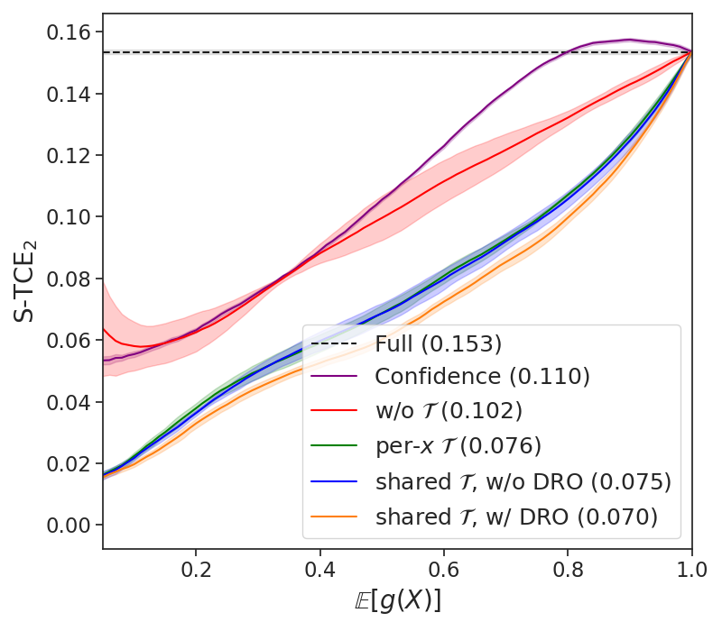
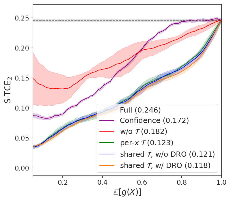
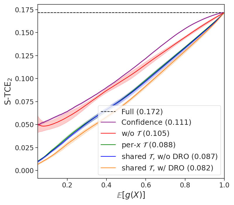
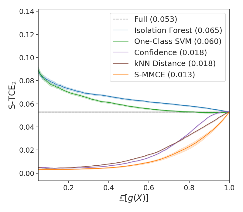
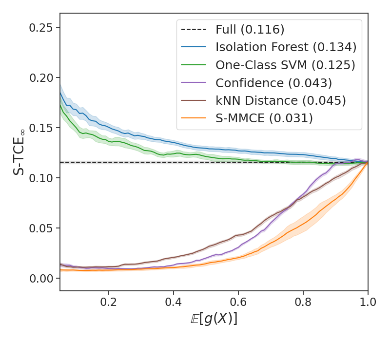
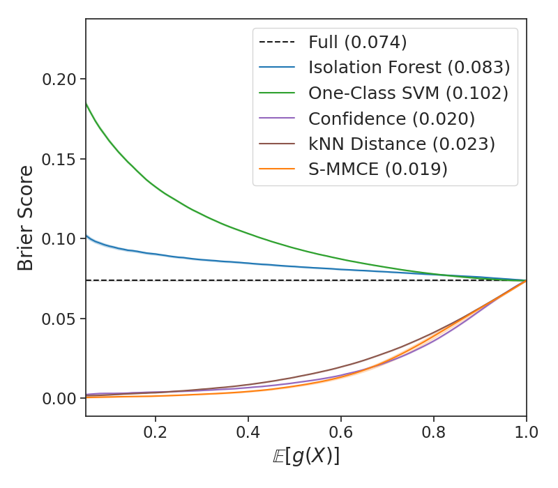
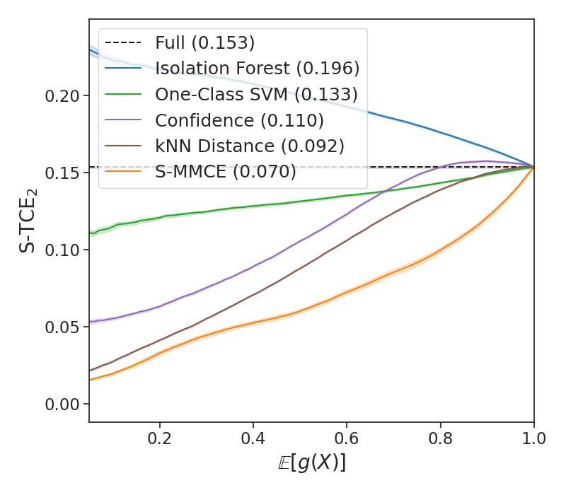
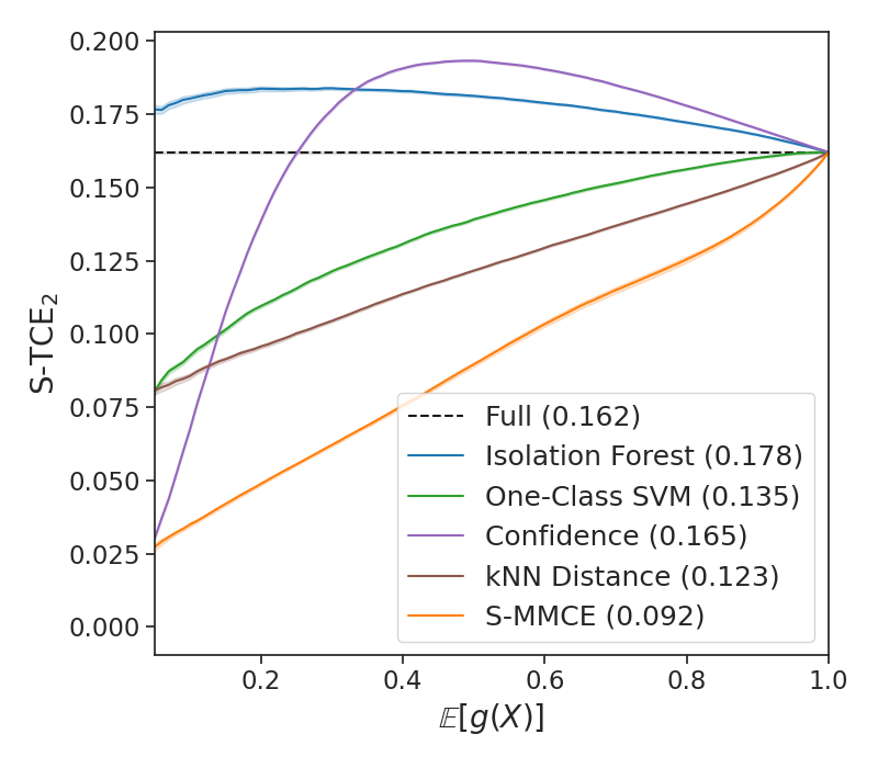
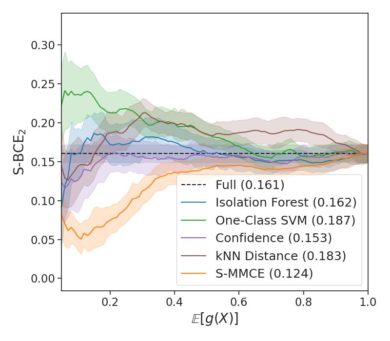
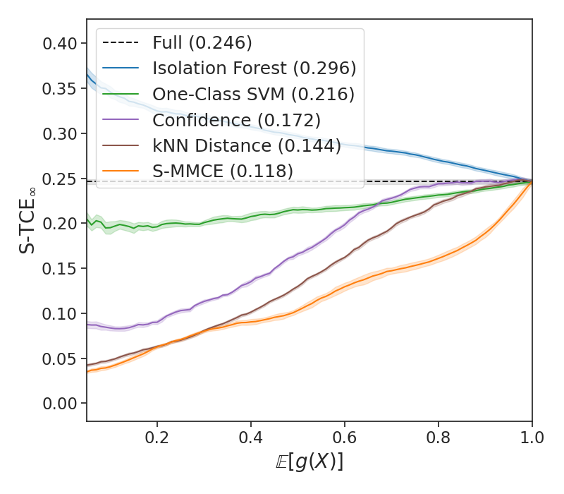
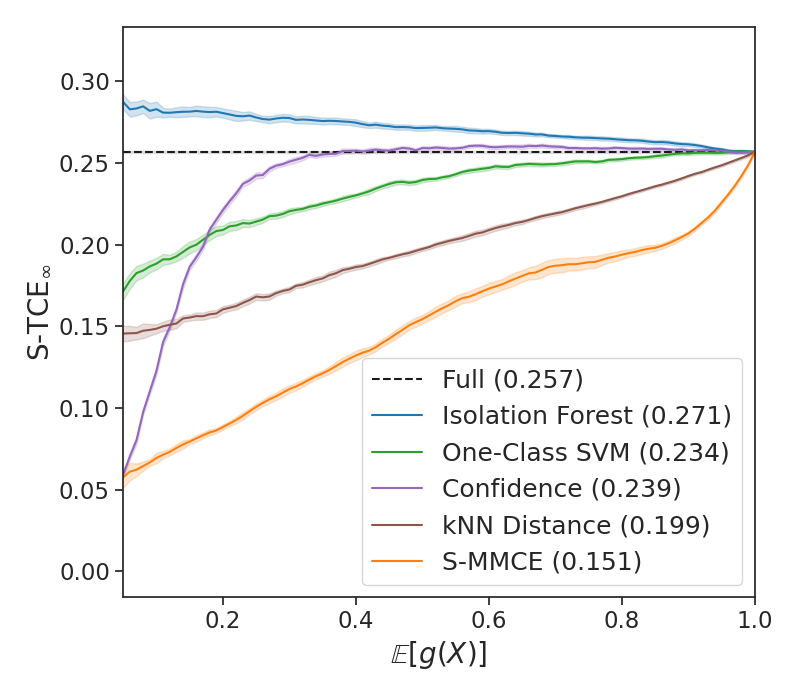
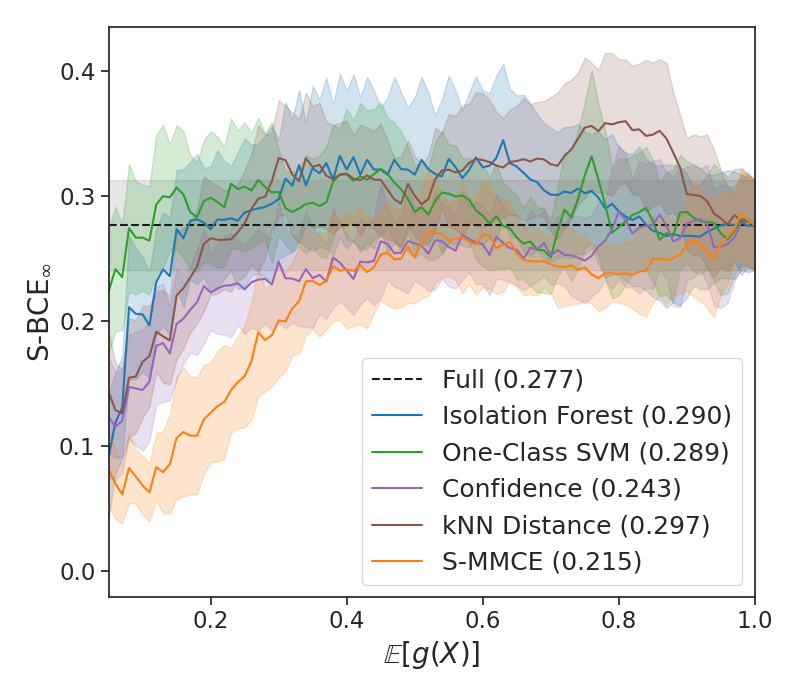
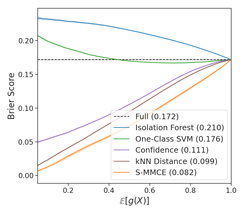
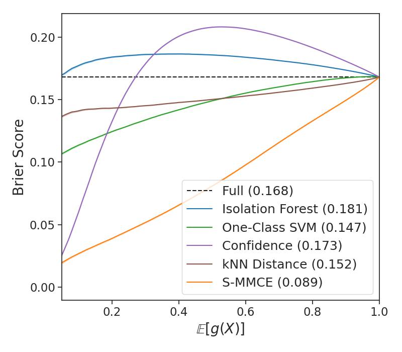
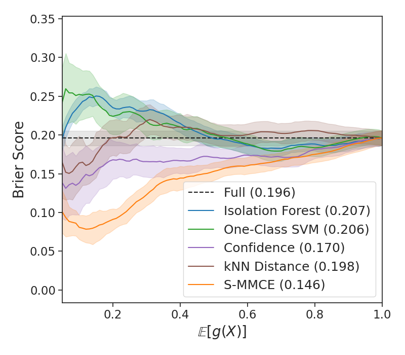
Selective calibration error.  Figure 3 reports our main calibration results. In all cases, we observe that optimizing for our S-MMCE objective leads to significant reductions in measured calibration error over the non-rejected examples. In particular, S-MMCE-derived scores outperform all baseline scoring mechanisms in both $\ell_{2}$ and $\ell_{\infty}$ Selective Calibration Error AUC, as well as in Brier Score AUC. This is most pronounced on the image classification tasks—which we conjecture is due to the effectiveness of AugMix perturbations at simulating the test-time shifts. Note that the lung cancer risk assessment task has far less data (both in training and testing) than CIFAR-10-C or ImageNet-C, hence its higher variance. Its perturbation class (reweighted resampling based on source hospital in the training set) is also relatively weak, and limited by the diversity of hospitals in NLST. Despite this, S-MMCE still substantially outperforms all baselines. Interestingly, while some baseline approaches—such as rejecting based on one-class SVM scores or isolation forest scores—can lead to worse calibration error than the full model without abstention, predictors produced using S-MMCE have reliably lower selective calibration error (per our goal) across all coverage rates $\xi$. The fact that our method significantly outperforms distance-based baselines, such as kNN distance or Isolation Forests, is also encouraging in that it suggests that $g$ has learned behaviors beyond identifying simple similarity to the training set.

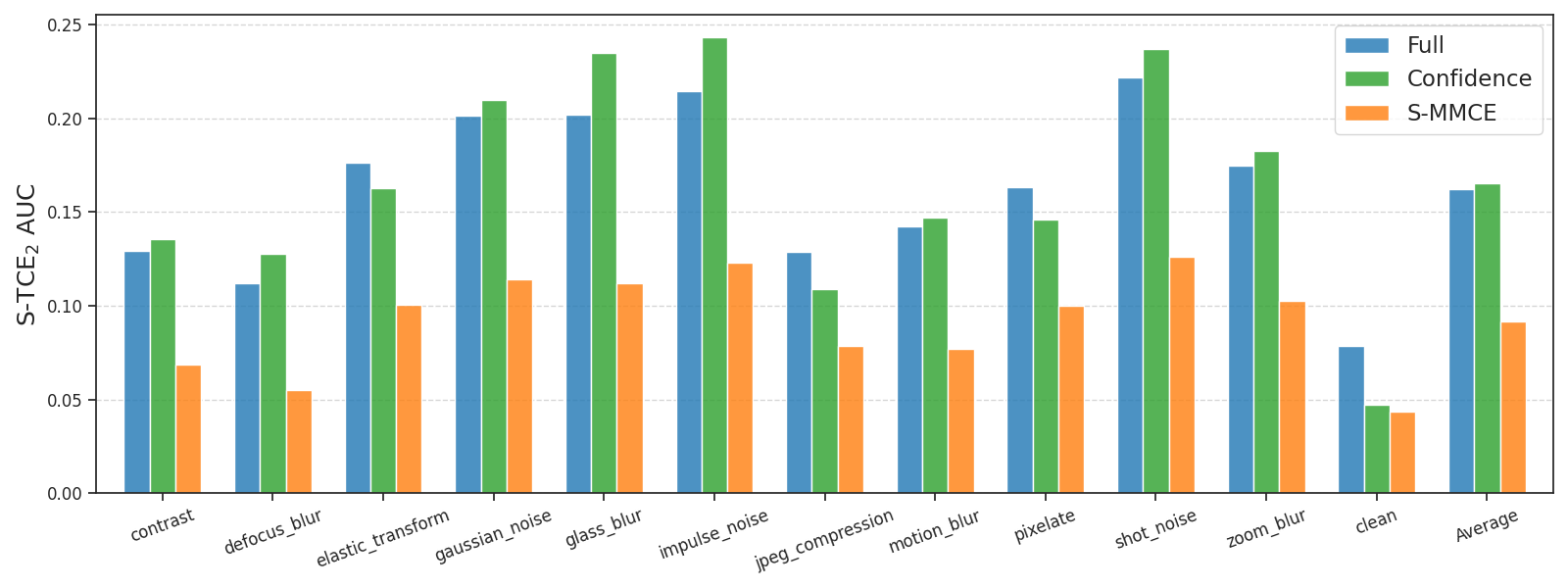
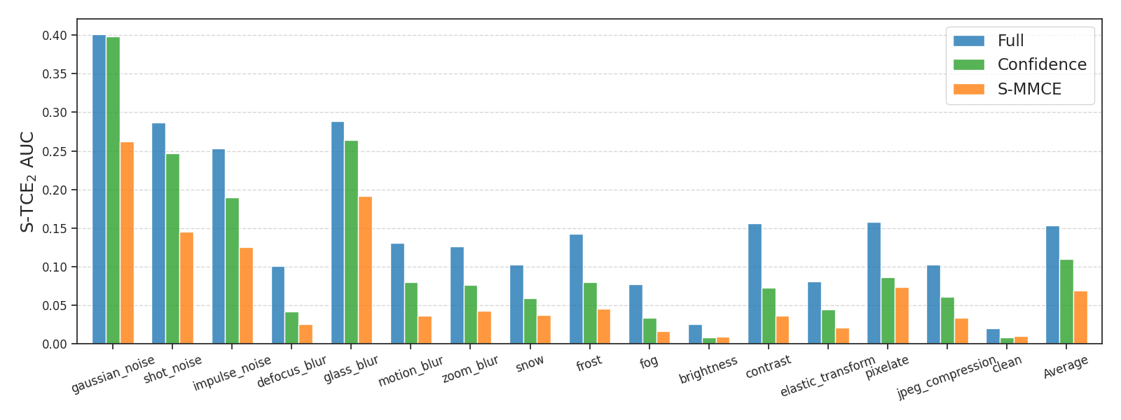
Robustness to perturbation type.  We are also interested to see how robust our selective mechanism is to the variety of types of test-time perturbation that we may face. Figure 2 shows a breakdown of Selective Calibration Error AUC across all 15 test time perturbations for CIFAR-10-C (note that Figure 3 shows only averages across all perturbations). Naturally, the reduction in calibration error is more pronounced when there is significant calibration error to begin with (see, for example, the Gaussian noise perturbation). That said, across all perturbation types, we observe substantial decreases in Selective Error AUC, both relative to the full model without abstentions, and relative to a standard confidence-based selection model. Similar results are also seen for ImageNet-C, which we provide in Appendix B.

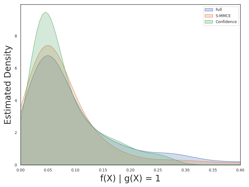
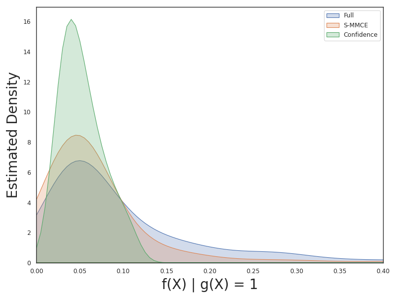
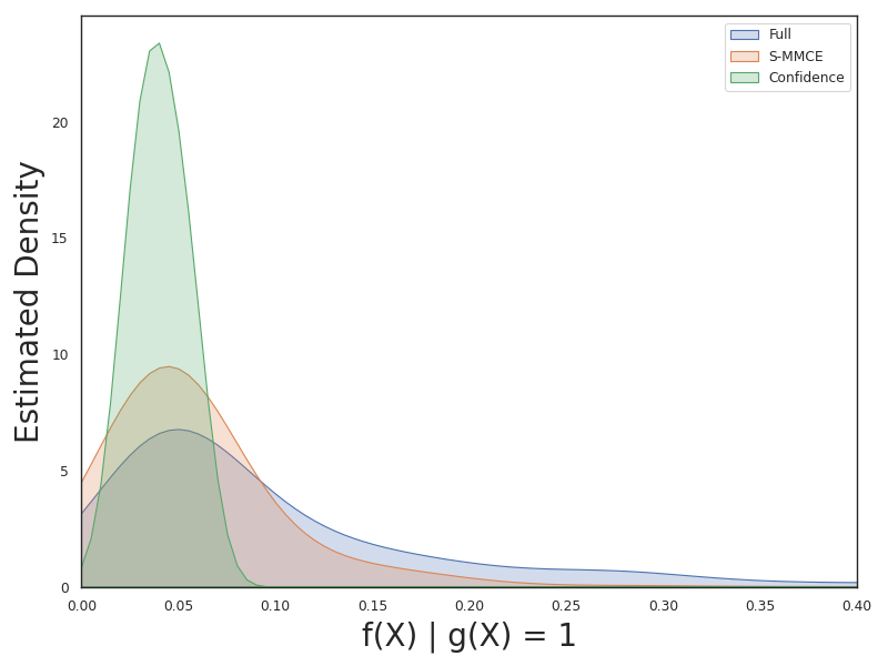
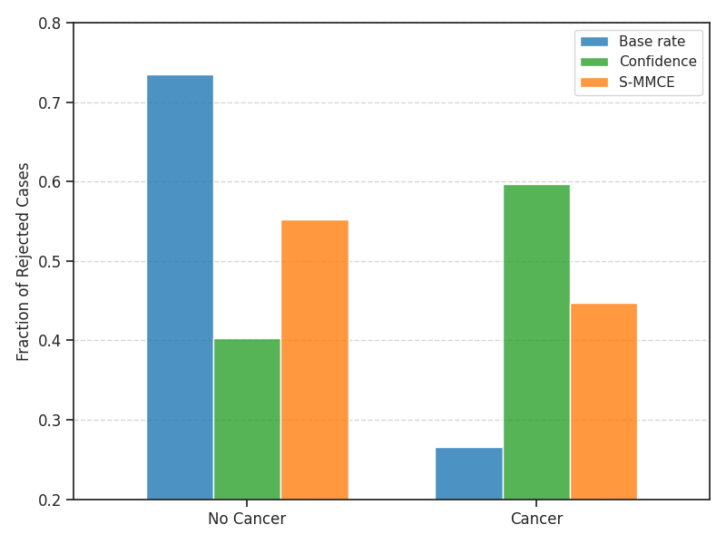
Analysis of rejection behavior.  We empirically investigate the types of selections that $g$ trained to optimize S-MMCE make, as compared to typical confidence-based selections. For the lung cancer risk assessment task on MGH data, Figure 4 shows the empirical distribution of confidence scores at various coverage levels $\xi$, conditioned on the example $X$ being selected ($g(X)=1$). As expected, the confidence-based method selects only the most confident examples, which in this case, is primarily examples where the patient is deemed least likely to be at risk ($f(X)\approx 0$). Figure 4 (b) then demonstrates that an undesirable outcome of this approach is that a disproportionate number of patients that do develop cancer ($Y=1$) are not serviced by the model ($g(X)=0$). In other words, the model avoids making wrong predictions on these patients, but as a result, doesn’t make predictions on the very examples it is needed most. On the other hand, our S-MMCE-based model clearly does not solely reject examples based on raw confidence—the distribution of confidence scores of accepted examples matches the marginal distribution (i.e., without rejection) much more closely. Similarly, as demonstrated in Figure 5, this selector rejects relatively fewer examples where $Y=1$ as compared to the confidence-based method. Together with the low calibration error results from Figure 3, this suggests that it is more capable of giving calibrated predictions both for non-cancerous and cancerous patients alike.

Ablations.  We highlight some additional results included in Appendix B. Figure B.2 presents an ablation study on CIFAR-10-C that explores the relative importance of different components of our main training procedure. Interestingly, even a selective model trained to minimize the S-MMCE on batches of in-domain data can achieve moderate improvements in selective calibration error on out-of-domain data, though the results are significantly further improved when adding in the perturbation family $\mathcal{T}$. Similarly, Figure B.3 shows the effect of first training the base model $f(X)$ on perturbations from the same family $\mathcal{T}$ (even though our focus, as stated in §1, is on black-box $f$).

Figure 5: A comparison of rejection ratios by label type at coverage $\xi=0.90$ on MGH data. Blue denotes the base ratio of each class in the full data. Proportionally more of the confidence-based rejections are cancerous (i.e., that we presume are “harder” to correctly classify). S-MMCE rejections are relatively less imbalanced relative to the natural rate.

Here, we use a model that is both trained and temperature scaled with AugMix perturbations over CIFAR-10. In line with Hendrycks et al. (2020), this leads to $f(X)$ with lower absolute calibration error on CIFAR-10-C. Nevertheless, our framework still leads to substantially lower selective calibration error AUC, relative to this new baseline.

Limitations and future work.  We acknowledge a few considerations that remain unaddressed in this work. First, marginal calibration, does not account for differences between sub-populations or individuals. This is both relevant to fairness and to personalized decision making Zhao et al. (2020); Shah et al. (2021); Jones et al. (2021). While we do not study them here, algorithms for more complete and unbiased notions of calibration Hebert-Johnson et al. (2018); Vaicenavicius et al. (2019); Shah et al. (2021), can be incorporated into our selective calibration framework. We also note that the performance of our method is strongly coupled with the perturbation family $\mathcal{T}$, which, here, is defined manually for each task. This can fail when the family $\mathcal{T}$ is not straightforward to construct. For example, the image augmentations such as those in AugMix Hendrycks et al. (2020) do not generalize across modalities (or even other image tasks, necessarily). Still, as automatic tools for creating synthetic augmentations improve, they can directly be included in our framework.

7 Conclusion

Reliable quantifications of model uncertainty can be critical to knowing when to trust deployed models, and how to base important decisions on the predictions that they make. Inevitably, deployed models will make mistakes. More fundamentally, not every query posed to even the best models can always be answered with complete certainty. In this paper, we introduced the concept of selective calibration, and proposed a framework for identifying when to abstain from making predictions that are potentially uncalibrated—i.e., when the model’s reported confidence levels may not accurately reflect the true probabilities of the predicted events. We showed that our method can be used to selectively make predictions that are better calibrated as a whole, while still being subject to basic coverage constraints. Finally, our experimental results demonstrated that (1) our calibrated selective classifiers make more complex abstention decisions than simple confidence-based selective classifiers, and (2) are able to generalize well under distribution shift.

Appendix A Technical details

A.1 Empirical calibration error

We use equal-mass binning Kumar et al. (2019); Roelofs et al. (2022) to estimate the expected calibration error. Specifically, given a dataset of confidence predictions, $\mathcal{D}_{\mathrm{test}}=\{(f(x_{1}),y_{1}),\ldots,(f(x_{n}),y_{n})\}$, we sort and assign each prediction pair $(f(x_{i}),y_{i})$ to one of $m$ equally sized bins $\mathcal{B}$ (i.e., bin $\mathcal{B}_{k}$ will contain all examples with scores falling in the $\frac{k-1}{m}\rightarrow\frac{k}{m}$ empirical quantiles). If $y$ is binary, the expected binary calibration error is estimated by

$$\text{BCE}\approx\left(\frac{1}{|\mathcal{B}|}\sum_{k=1}^{|\mathcal{B}|}\left(\frac{\sum_{i\in\mathcal{B}_{k}}y_{i}}{|\mathcal{B}_{k}|}-\frac{\sum_{i\in\mathcal{B}_{k}}f(x_{i})}{|\mathcal{B}_{k}|}\right)^{q}\right)^{\frac{1}{q}}.$$ (18)

When $y$ is multi-class, we replace $y_{i}$ and $f(x_{i})$ in Eq. (18) with $\mathbf{1}\{y_{i}=\arg\!\max_{y\in[K]}f(x_{i})_{y}\}$ and $\max_{y\in[K]}f(x_{i})_{y}$, respectively to compute the TCE. We set the number of bins $m$ to $\min(15,\lfloor\frac{n}{25}\rfloor)$. For selective calibration error, we first filter $\mathcal{D}_{\mathrm{test}}$ to only include the examples that have $g(X_{i})=1$, and then apply the same binning procedure.

A.2 Training details

We use a Laplace kernel with $\sigma=0.2$ for our choice of universal kernel $k$ in S-MMCE. All models are trained in PyTorch, while high-level input features for $g$ are computed with sklearn. We compute the S-MMCE with samples of size 1024 (of examples with the same perturbation $t\in\mathcal{T}$ applied), with a combined batch size of $m=32$. We train all models for 5 epochs, with 50k examples per epoch (7.8k updates total). The loss weight hyper-parameters $\lambda_{1}$ and $\lambda_{2}$ were set to $|\mathcal{D}|$ = 1024 and 1e-3, respectively. $\kappa$, in our top-$\kappa$ calibration error loss, is set to 4. Our code will be made available at www.github.com/ajfisch/calibrated-selection.

A.3 NLST-MGH lung cancer data

The CT scans in the NLST data are low-dose CT scans, and from patients specifically enrolled in lung cancer screening programs across the 33 participating hospitals. The MGH test data, on the other hand, is aggregated across a diverse assortment of all patients in their system who underwent any type of chest CT between 2008-2018, and matched NLST enrollment criteria (55-74 years old, current or former smokers with 30+ pack years). Note that since these patients are not enrolled in a regular screening program, not all patients have complete 6-year follow-up records. All patients without documented cancer diagnosis in the 2008-2018 period are assumed to be cancer-free.

Appendix B Additional results

In this section, we present a number of additional experimental results. Figure B.1 present results per perturbation type on ImageNet-C. Like CIFAR-10-C (Figure 2), we see consistent and significant selective calibration error reduction across perturbation types. This is in contrast to the confidence-based selective classifier, which does not always reliably lead to improved selective calibration error. Figure B.2 presents the results of an ablation study on CIFAR-10-C. Specifically, we look at the effect of not including any perturbations, including perturbations on an example level only (i.e., $t(x)$ rather than $t\circ\mathcal{D}_{\mathrm{train}}$), and using all perturbations in a batch instead of only the $\kappa$-worst. Interestingly, even training the S-MMCE loss only on in-domain, unperturbed data can lead to moderate improvements in selective calibration error. Including perturbations, however, leads to significantly better results. Sharing perturbations across batches or training on the $\kappa$-worst then offer additional, but only small, improvements.

Figure B.1: $\ell_{2}$ selective top-label calibration error (S-TCE₂) AUC, reported for each of the 11 test-time perturbations in ImageNet-C (in addition to the average). Across perturbation types, optimizing for S-MMCE consistently leads to significant error reductions relative to a model without abstentions ("Full"), as well as the standard selective classifier ("Confidence"). In contrast, the confidence-based selective classifier can sometimes lead to worse calibration error.

Figure B.2: Ablation results on CIFAR-10-C for different configurations of our method. Without $\mathcal{T}$: no perturbations. Per-$x$ $\mathcal{T}$: perturbations are mixed within a batch. Shared $\mathcal{T}$, without DRO: update on all batches, not just the $\kappa$-worst. Shared $\mathcal{T}$, with DRO: update only on the $\kappa$ worst examples per batch (our standard algorithm).

Figure B.3: Results on CIFAR-10-C averaged over perturbation types when including AugMix pertubrations ($\mathcal{T}$) during the original training of $f(X)$. As also first reported in Hendrycks et al. (2020), including such perturbations during training indeed reduces calibration error out-of-the-box. Using even the same perturbation class $\mathcal{T}$ during selective training, can yield a selective classifier with substantially lower relative calibration error.

References

- Aberle et al. (2011) Denise R Aberle, Amanda M Adams, Christine D Berg, William C Black, Jonathan D Clapp, Richard M Fagerstrom, Ilana F Gareen, Constantine Gatsonis, Pamela M Marcus, JoRean D Sicks, National Lung Screening Trial Research Team, and Reginald F. Munden. Reduced lung-cancer mortality with low-dose computed tomographic screening. New England Journal of Medicine, 365(5):395–409, 2011.
- Amodei et al. (2016) Dario Amodei, Chris Olah, Jacob Steinhardt, Paul Christiano, John Schulman, and Dan Mané. Concrete problems in ai safety. ArXiv preprint: 1606.06565, 2016.
- Angelopoulos et al. (2022) Anastasios N. Angelopoulos, Stephen Bates, Adam Fisch, Lihua Lei, and Tal Schuster. Conformal risk control. 2022.
- Ashukha et al. (2020) Arsenii Ashukha, Alexander Lyzhov, Dmitry Molchanov, and Dmitry Vetrov. Pitfalls of in-domain uncertainty estimation and ensembling in deep learning. In International Conference on Learning Representations (ICLR), 2020.
- Bao & Barzilay (2022) Yujia Bao and Regina Barzilay. Learning to split for automatic bias detection. ArXiv preprint: 2204.13749, 2022.
- Bartlett & Wegkamp (2008) Peter L. Bartlett and Marten H. Wegkamp. Classification with a reject option using a hinge loss. Journal of Machine Learning Research, 9(59):1823–1840, 2008.
- Bates et al. (2020) Stephen Bates, Anastasios Nikolas Angelopoulos, Lihua Lei, Jitendra Malik, and Michael I. Jordan. Distribution free, risk controlling prediction sets. ArXiv preprint: 2101.02703, 2020.
- Bertsekas (1996) Dimitri P. Bertsekas. Constrained Optimization and Lagrange Multiplier Methods (Optimization and Neural Computation Series). Athena Scientific, 1 edition, 1996. ISBN 1886529043.
- Brier (1950) Glenn W. Brier. Verification of forecasts expressed in terms of probability. Monthly Weather Review, 78:1–3, 1950.
- Buslaev et al. (2020) Alexander Buslaev, Vladimir I. Iglovikov, Eugene Khvedchenya, Alex Parinov, Mikhail Druzhinin, and Alexandr A. Kalinin. Albumentations: Fast and flexible image augmentations. Information, 11(2), 2020.
- Cauchois et al. (2020) Maxime Cauchois, Suyash Gupta, Alnur Ali, and John C. Duchi. Robust validation: Confident predictions even when distributions shift. ArXiv preprint: 2008.04267, 2020.
- Charoenphakdee et al. (2021) Nontawat Charoenphakdee, Zhenghang Cui, Yivan Zhang, and Masashi Sugiyama. Classification with rejection based on cost-sensitive classification. In International Conference on Machine Learning (ICML), 2021.
- Chen et al. (2020) Ting Chen, Simon Kornblith, Mohammad Norouzi, and Geoffrey Hinton. A simple framework for contrastive learning of visual representations. In International Conference on Machine Learning (ICML), 2020.
- Chow (1957) C. K. Chow. An optimum character recognition system using decision functions. IRE Transactions on Electronic Computers, 6:247–254, 1957.
- Choy et al. (2018) Garry Choy, Omid Khalilzadeh, Mark Michalski, Synho Do, Anthony E. Samir, Oleg S. Pianykh, J. Raymond Geis, Pari V. Pandharipande, James A. Brink, and Keith J. Dreyer. Current applications and future impact of machine learning in radiology. Radiology, 288(2):318–328, 2018.
- Chwialkowski et al. (2015) Kacper P Chwialkowski, Aaditya Ramdas, Dino Sejdinovic, and Arthur Gretton. Fast two-sample testing with analytic representations of probability measures. In Advances in Neural Information Processing Systems (NeurIPS), 2015.
- Cordella et al. (1995) L.P. Cordella, C. De Stefano, F. Tortorella, and M. Vento. A method for improving classification reliability of multilayer perceptrons. IEEE Transactions on Neural Networks, 6(5):1140–1147, 1995. doi: 10.1109/72.410358.
- Cortes et al. (2016a) Corinna Cortes, Giulia DeSalvo, and Mehryar Mohri. Boosting with abstention. In Advances in Neural Information Processing Systems (NeurIPS), 2016a.
- Cortes et al. (2016b) Corinna Cortes, Giulia DeSalvo, and Mehryar Mohri. Learning with rejection. In International Conference on Algorithmic Learning Theory (ALT), 2016b.
- Cubuk et al. (2020) Ekin Dogus Cubuk, Barret Zoph, Jon Shlens, and Quoc Le. Randaugment: Practical automated data augmentation with a reduced search space. In Advances in Neural Information Processing Systems (NeurIPS), 2020.
- Dawid (1982) A. P. Dawid. The well-calibrated bayesian. Journal of the American Statistical Association, 77(379):605–610, 1982.
- De Stefano et al. (2000) Claudio De Stefano, Carlo Sansone, and Mario Vento. To reject or not to reject: That is the question - an answer in case of neural classifiers. IEEE Transactions on Systems, Man, and Cybernetics, Part C (Applications and Reviews), 30:84 – 94, 03 2000.
- DeGroot & Fienberg (1983) Morris H. DeGroot and Stephen E. Fienberg. The comparison and evaluation of forecasters. Journal of the Royal Statistical Society. Series D (The Statistician), 32(1/2):12–22, 1983.
- Deng et al. (2009) Jia Deng, Wei Dong, Richard Socher, Li-Jia Li, Kai Li, and Li Fei-Fei. Imagenet: A large-scale hierarchical image database. In Conference on Computer Vision and Pattern Recognition (CVPR), 2009.
- Dromain et al. (2013) C. Dromain, B. Boyer, R. Ferré, S. Canale, S. Delaloge, and C. Balleyguier. Computed-aided diagnosis (cad) in the detection of breast cancer. European Journal of Radiology, 82(3):417–423, 2013.
- El-Yaniv & Wiener (2010) Ran El-Yaniv and Yair Wiener. On the foundations of noise-free selective classification. Journal of Machine Learning Research (JMLR), 11, 2010.
- Foster & Vohra (1998) Dean P. Foster and Rakesh V. Vohra. Asymptotic calibration. Biometrika, 85(2):379–390, 1998.
- Geifman & El-Yaniv (2017) Yonatan Geifman and Ran El-Yaniv. Selective classification for deep neural networks. In Advances in Neural Information Processing Systems (NeurIPS), 2017.
- Geifman & El-Yaniv (2019) Yonatan Geifman and Ran El-Yaniv. SelectiveNet: A deep neural network with an integrated reject option. In International Conference on Machine Learning (ICML), 2019.
- Ginart et al. (2022) Tony Ginart, Martin Jinye Zhang, and James Zou. MLDemon: Deployment monitoring for machine learning systems. In International Conference on Artificial Intelligence and Statistics (AISTATS), 2022.
- Gneiting et al. (2007) Tilmann Gneiting, Fadoua Balabdaoui, and Adrian E. Raftery. Probabilistic forecasts, calibration and sharpness. Journal of the Royal Statistical Society Series B, 69(2):243–268, 2007.
- Gretton et al. (2012) Arthur Gretton, Karsten M. Borgwardt, Malte J. Rasch, Bernhard Schölkopf, and Alexander Smola. A kernel two-sample test. Journal of Machine Learning Research (JMLR), 13(25):723–773, 2012.
- Guo et al. (2017a) Chuan Guo, Geoff Pleiss, Yu Sun, and Kilian Q. Weinberger. On calibration of modern neural networks. In International Conference on Machine Learning (ICML), 2017a.
- Guo et al. (2017b) Chuan Guo, Geoff Pleiss, Yu Sun, and Kilian Q. Weinberger. On calibration of modern neural networks. In International Conference on Machine Learning (ICML), 2017b.
- Gupta & Ramdas (2022) Chirag Gupta and Aaditya Ramdas. Top-label calibration and multiclass-to-binary reductions. In International Conference on Learning Representations (ICLR), 2022.
- Gupta et al. (2020) Chirag Gupta, Aleksandr Podkopaev, and Aaditya Ramdas. Distribution-free binary classification: prediction sets, confidence intervals and calibration. In Advances in Neural Information Processing Systems (NeurIPS), 2020.
- He et al. (2016) Kaiming He, Xiangyu Zhang, Shaoqing Ren, and Jian Sun. Deep residual learning for image recognition. In IEEE Conference on Computer Vision and Pattern Recognition (CVPR), 2016.
- Hebert-Johnson et al. (2018) Ursula Hebert-Johnson, Michael Kim, Omer Reingold, and Guy Rothblum. Multicalibration: Calibration for the (Computationally-identifiable) masses. In International Conference on Machine Learning (ICML), 2018.
- Hellman (1970) Martin E. Hellman. The nearest neighbor classification rule with a reject option. IEEE Transactions on Systems Science and Cybernetics, 6:179–185, 1970.
- Hendrycks & Dietterich (2019) Dan Hendrycks and Thomas Dietterich. Benchmarking neural network robustness to common corruptions and perturbations. International Conference on Learning Representations (ICLR), 2019.
- Hendrycks et al. (2020) Dan Hendrycks, Norman Mu, Ekin D. Cubuk, Barret Zoph, Justin Gilmer, and Balaji Lakshminarayanan. AugMix: A simple data processing method to improve robustness and uncertainty. Proceedings of the International Conference on Learning Representations (ICLR), 2020.
- Herbei & Wegkamp (2006) Radu Herbei and Marten H. Wegkamp. Classification with reject option. Canadian Journal of Statistics, 34(4):709–721, 2006.
- Jiang et al. (2018) Heinrich Jiang, Been Kim, Melody Guan, and Maya Gupta. To trust or not to trust a classifier. In Advances in Neural Information Processing Systems (NeurIPS), 2018.
- Jiang et al. (2012) Xiaoqian Jiang, Melanie Osl, Jihoon Kim, and Lucila Ohno-Machado. Calibrating predictive model estimates to support personalized medicine. Journal of the American Medical Informatics Association, 19(2):263–274, 2012.
- Jones et al. (2021) Erik Jones, Shiori Sagawa, Pang Wei Koh, Ananya Kumar, and Percy Liang. Selective classification can magnify disparities across groups. In International Conference on Learning Representations (ICLR), 2021.
- Kamath et al. (2020) Amita Kamath, Robin Jia, and Percy Liang. Selective question answering under domain shift. In Annual Meeting of the Association for Computational Linguistics (ACL), 2020.
- Karandikar et al. (2021) Archit Karandikar, Nicholas Cain, Dustin Tran, Balaji Lakshminarayanan, Jonathon Shlens, Michael Curtis Mozer, and Rebecca Roelofs. Soft calibration objectives for neural networks. In Advances in Neural Information Processing Systems (NeurIPS), 2021.
- Kawaguchi & Lu (2020) Kenji Kawaguchi and Haihao Lu. Ordered sgd: A new stochastic optimization framework for empirical risk minimization. In International Conference on Artificial Intelligence and Statistics (AISTATS), 2020.
- Koh et al. (2021) Pang Wei Koh, Shiori Sagawa, Henrik Marklund, Sang Michael Xie, Marvin Zhang, Akshay Balsubramani, Weihua Hu, Michihiro Yasunaga, Richard Lanas Phillips, Irena Gao, Tony Lee, Etienne David, Ian Stavness, Wei Guo, Berton Earnshaw, Imran Haque, Sara M Beery, Jure Leskovec, Anshul Kundaje, Emma Pierson, Sergey Levine, Chelsea Finn, and Percy Liang. Wilds: A benchmark of in-the-wild distribution shifts. In International Conference on Machine Learning (ICML), 2021.
- Krizhevsky (2012) Alex Krizhevsky. Learning multiple layers of features from tiny images. University of Toronto, 2012.
- Kuleshov & Liang (2015) Volodymyr Kuleshov and Percy Liang. Calibrated structured prediction. In Advances in Neural Information Processing Systems (NeurIPS), 2015.
- Kuleshov et al. (2018) Volodymyr Kuleshov, Nathan Fenner, and Stefano Ermon. Accurate uncertainties for deep learning using calibrated regression. In International Conference on Machine Learning (ICML), 2018.
- Kull et al. (2019) Meelis Kull, Miquel Perelló-Nieto, Markus Kängsepp, Telmo de Menezes e Silva Filho, Hao Song, and Peter A. Flach. Beyond temperature scaling: Obtaining well-calibrated multi-class probabilities with dirichlet calibration. In Advances in Neural Information Processing (NeurIPS), 2019.
- Kumar et al. (2019) Ananya Kumar, Percy Liang, and Tengyu Ma. Verified uncertainty calibration. In Advances in Neural Information Processing Systems (NeurIPS), 2019.
- Kumar et al. (2018) Aviral Kumar, Sunita Sarawagi, and Ujjwal Jain. Trainable calibration measures for neural networks from kernel mean embeddings. In International Conference on Machine Learning (ICML), 2018.
- Levy et al. (2020) Daniel Levy, Yair Carmon, John C Duchi, and Aaron Sidford. Large-scale methods for distributionally robust optimization. In Advances in Neural Information Processing Systems (NeurIPS), 2020.
- Lipton et al. (2018) Zachary Lipton, Yu-Xiang Wang, and Alexander Smola. Detecting and correcting for label shift with black box predictors. In International Conference on Machine Learning (ICML), 2018.
- Liu et al. (2021) Evan Z Liu, Behzad Haghgoo, Annie S Chen, Aditi Raghunathan, Pang Wei Koh, Shiori Sagawa, Percy Liang, and Chelsea Finn. Just train twice: Improving group robustness without training group information. In Proceedings of the 38th International Conference on Machine Learning (ICML), 2021.
- Liu et al. (2008) Fei Tony Liu, Kai Ming Ting, and Zhi-Hua Zhou. Isolation forest. In IEEE International Conference on Data Mining, 2008.
- Mikhael et al. (2022) Peter G. Mikhael, Jeremy Wohlwend, Ludvig Karstens Adam Yala, Justin Xiang, Angelo K. Takigami, Patrick P. Bourgouin, PuiYee Chan, Sofiane Mrah, Wael Amayri, Yu-Hsiang Juan, Cheng-Ta Yang, Yung-Liang Wan, Gigin Lin, Lecia V. Sequist, Florian J. Fintelmann, and Regina Barzilay. Sybil: A validated deep learning model to predict future lung cancer risk from a single low-dose chest computed tomography, 2022.
- Minderer et al. (2021) Matthias Minderer, Josip Djolonga, Rob Romijnders, Frances Ann Hubis, Xiaohua Zhai, Neil Houlsby, Dustin Tran, and Mario Lucic. Revisiting the calibration of modern neural networks. In Advances in Neural Information Processing Systems (NeurIPS), 2021.
- Mozannar & Sontag (2020) Hussein Mozannar and David Sontag. Consistent estimators for learning to defer to an expert. In International Conference on Machine Learning (ICML), 2020.
- Mukhoti et al. (2020) Jishnu Mukhoti, Viveka Kulharia, Amartya Sanyal, Stuart Golodetz, Philip Torr, and Puneet Dokania. Calibrating deep neural networks using focal loss. In Advances in Neural Information Processing Systems (NeurIPS), 2020.
- Murphy (1973) Allan H. Murphy. A new vector partition of the probability score. Journal of Applied Meteorology (1962-1982), 12(4):595–600, 1973.
- Murphy & Epstein (1967) Allan H. Murphy and Edward S. Epstein. Verification of probabilistic predictions: A brief review. Journal of Applied Meteorology and Climatology, 6(5):748 – 755, 1967.
- Niculescu-Mizil & Caruana (2005) Alexandru Niculescu-Mizil and Rich Caruana. Predicting good probabilities with supervised learning. In International Conference on Machine Learning (ICML), 2005.
- Nixon et al. (2019) Jeremy Nixon, Mike Dusenberry, Linchuan Zhang, Ghassen Jerfel, and Dustin Tran. Measuring calibration in deep learning. ArXiv preprint: 1904.01685, 2019.
- Ovadia et al. (2019) Yaniv Ovadia, Emily Fertig, Jie Ren, Zachary Nado, D. Sculley, Sebastian Nowozin, Joshua Dillon, Balaji Lakshminarayanan, and Jasper Snoek. Can you trust your model's uncertainty? evaluating predictive uncertainty under dataset shift. In Advances in Neural Information Processing Systems (NeurIPS), 2019.
- Park et al. (2022) Sangdon Park, Edgar Dobriban, Insup Lee, and Osbert Bastani. PAC prediction sets under covariate shift. In International Conference on Learning Representations (ICLR), 2022.
- Platt (1999) John C. Platt. Probabilistic outputs for support vector machines and comparisons to regularized likelihood methods. In Advances in Large Margin Classifiers, pp. 61–74. MIT Press, 1999.
- Quionero-Candela et al. (2009) Joaquin Quionero-Candela, Masashi Sugiyama, Anton Schwaighofer, and Neil D. Lawrence. Dataset Shift in Machine Learning. The MIT Press, 2009. ISBN 0262170051.
- Rabanser et al. (2019) Stephan Rabanser, Stephan Günnemann, and Zachary Lipton. Failing loudly: An empirical study of methods for detecting dataset shift. In Advances in Neural Information Processing Systems (NeurIPS), 2019.
- Reddi et al. (2015) Sashank Reddi, Barnabas Poczos, and Alex Smola. Doubly robust covariate shift correction. In AAAI Conference on Artificial Intelligence, 2015.
- Roelofs et al. (2022) Rebecca Roelofs, Nicholas Cain, Jonathon Shlens, and Michael C. Mozer. Mitigating bias in calibration error estimation. In Proceedings of The 25th International Conference on Artificial Intelligence and Statistics (AISTATS), 2022.
- Rusak et al. (2020) Evgenia Rusak, Lukas Schott, Roland S. Zimmermann, Julian Bitterwolf, Oliver Bringmann, Matthias Bethge, and Wieland Brendel. A simple way to make neural networks robust against diverse image corruptions. In European Conference on Computer Vision (ECCV), 2020.
- Sagawa et al. (2020) Shiori Sagawa, Pang Wei Koh, Tatsunori B. Hashimoto, and Percy Liang. Distributionally robust neural networks. In International Conference on Learning Representations (ICLR), 2020.
- Schölkopf et al. (2001) Bernhard Schölkopf, John C. Platt, John C. Shawe-Taylor, Alex J. Smola, and Robert C. Williamson. Estimating the support of a high-dimensional distribution. Neural Computation, 13(7):1443–1471, 2001.
- Shah et al. (2021) Abhin Shah, Yuheng Bu, Joshua Ka-Wing Lee, Subhro Das, Rameswar Panda, Prasanna Sattigeri, and Gregory W Wornell. Selective regression under fairness criteria. arXiv preprint arXiv:2110.15403, 2021.
- Shaked & Shanthikumar (2007) M. Shaked and J.G. Shanthikumar. Stochastic Orders. Springer Series in Statistics. Springer New York, 2007. ISBN 9780387346755.
- Sugiyama & Müller (2005) Masashi Sugiyama and Klaus-Robert Müller. Input-dependent estimation of generalization error under covariate shift. Statistics and Decisions, 23(4):249–279, 2005.
- Tibshirani et al. (2019) Ryan J Tibshirani, Rina Foygel Barber, Emmanuel Candès, and Aaditya Ramdas. Conformal prediction under covariate shift. In Advances in Neural Information Processing Systems (NeurIPS), 2019.
- Tran et al. (2022) Dustin Tran, Jeremiah Liu, Michael W. Dusenberry, Du Phan, Mark Collier, Jie Ren, Kehang Han, Zi Wang, Zelda Mariet, Huiyi Hu, Neil Band, Tim G. J. Rudner, Karan Singhal, Zachary Nado, Joost van Amersfoort, Andreas Kirsch, Rodolphe Jenatton, Nithum Thain, Honglin Yuan, Kelly Buchanan, Kevin Murphy, D. Sculley, Yarin Gal, Zoubin Ghahramani, Jasper Snoek, and Balaji Lakshminarayanan. Plex: Towards reliability using pretrained large model extensions. 2022.
- Tsoukalas et al. (2015) Athanasios Tsoukalas, Timothy Albertson, and Ilias Tagkopoulos. From data to optimal decision making: A data-driven, probabilistic machine learning approach to decision support for patients with sepsis. JMIR Medical Informatics, 3(1):e11, 2015.
- Vaicenavicius et al. (2019) Juozas Vaicenavicius, David Widmann, Carl Andersson, Fredrik Lindsten, Jacob Roll, and Thomas Schön. Evaluating model calibration in classification. In International Conference on Artificial Intelligence and Statistics (AISTATS), 2019.
- van Amersfoort et al. (2020) Joost van Amersfoort, Lewis Smith, Yee Whye Teh, and Yarin Gal. Uncertainty estimation using a single deep deterministic neural network. In International Conference on Machine Learning (ICML), 2020.
- Vovk et al. (2003) Vladimir Vovk, Ilia Nouretdinov, and Alexander Gammerman. Testing exchangeability on-line. In ICML, 2003.
- Vovk et al. (2005) Vladimir Vovk, Alex Gammerman, and Glenn Shafer. Algorithmic Learning in a Random World. Springer-Verlag, Berlin, Heidelberg, 2005.
- Wald et al. (2021) Yoav Wald, Amir Feder, Daniel Greenfeld, and Uri Shalit. On calibration and out-of-domain generalization. In Advances in Neural Information Processing Systems (NeurIPS), 2021.
- Wen et al. (2014) Junfeng Wen, Chun-Nam Yu, and Russell Greiner. Robust learning under uncertain test distributions: Relating covariate shift to model misspecification. In International Conference on Machine Learning (ICML), 2014.
- Widmann et al. (2019) David Widmann, Fredrik Lindsten, and Dave Zachariah. Calibration tests in multi-class classification: A unifying framework. In Advances in Neural Information Processing Systems (NeurIPS), 2019.
- Wiener & El-Yaniv (2012) Yair Wiener and Ran El-Yaniv. In Advances in Neural Information Processing Systems (NeurIPS), 2012.
- Yu et al. (2022) Yaodong Yu, Stephen Bates, Yi Ma, and Michael I Jordan. Robust calibration with multi-domain temperature scaling. arXiv preprint arXiv:2206.02757, 2022.
- Zadrozny & Elkan (2001) Bianca Zadrozny and Charles Elkan. Obtaining calibrated probability estimates from decision trees and naive bayesian classifiers. In International Conference on Machine Learning (ICML), 2001.
- Zagoruyko & Komodakis (2016) Sergey Zagoruyko and Nikos Komodakis. Wide residual networks. In British Machine Vision Conference (BMVC), 2016.
- Zhao et al. (2020) Shengjia Zhao, Tengyu Ma, and Stefano Ermon. Individual calibration with randomized forecasting. In International Conference on Machine Learning (ICML), 2020.
- Zhao et al. (2021) Shengjia Zhao, Michael Kim, Roshni Sahoo, Tengyu Ma, and Stefano Ermon. Calibrating predictions to decisions: A novel approach to multi-class calibration. In Advances in Neural Information Processing Systems (NeurIPS), 2021.