A Novel SCA-Based Method for Beamforming Optimization in IRS/RIS-Assisted MU-MISO Downlink

Abstract

In this letter, we consider the fundamental problem of jointly designing the transmit beamformers and the phase-shifts of the intelligent reflecting surface (IRS) / reconfigurable intelligent surface (RIS) to minimize the transmit power, subject to quality-of-service constraints at individual users in an IRS-assisted multiuser multiple-input single-output downlink communication system. In particular, we propose a new successive convex approximation based second-order cone programming approach in which all the optimization variables are simultaneously updated in each iteration. Our proposed scheme achieves superior performance compared to state-of-the-art benchmark solutions. In addition, the complexity of the proposed scheme is $O(N_{\mathrm{s}}^{3.5})$, while that of state-of-the-art benchmark schemes is $O(N_{\mathrm{s}}^{7})$, where $N_{\mathrm{s}}$ denotes the number of reflecting elements at the IRS.

I Introduction

With the recent advancement in metamaterials, intelligent reflecting surfaces (IRSs) or reconfigurable intelligent surfaces (RISs) are being envisioned as one of the key enabling technologies for the next-generation wireless communication systems [1, 2, 3, 4, 5]. The problem of transmit power minimization (PowerMin) for IRS-assisted systems is of fundamental interest to reduce the system power consumption [6]. In this context, the authors of [7, 8, 9] considered the PowerMin problem in IRS-assisted multiuser single-input single-output (MU-SISO) downlink and multiuser single-input multiple-output (MU-SIMO) uplink systems. Compared to traditional systems, the PowerMin problem is more challenging to solve in the presence of IRSs due to the coupling between the transmit beamformer(s) and the phase shifts of the IRS. In particular, the PowerMin problem in IRS-assisted multiuser multiple-input single-output (MU-MISO) downlink systems for different scenarios, including multicasting [10], broadcasting [11], symbol-level precoding [12], millimeter-wave systems [13], and simultaneous wireless information and power transfer (SWIPT) system [14], were recently addressed in the literature.

In the existing literature [11, 14, 9, 13, 12, 10], the prevailing method for solving the PowerMin problem is to alternately optimize the transmit beamformer and the IRS phase-shifts, with one of them kept fixed. Although alternating optimization (AO) greatly simplifies the optimization problem, it may not yield a high-performance solution due to the intricate coupling among the design variables. From the point of view of the computational complexity, another limitation of existing solutions to the PowerMin problem in IRS-assisted MU-MISO systems is the extensive use of semidefinite relaxation (SDR) [10, (P7)], [11, (P4’)] which incurs very high computational complexity, and is thus not suitable for large-scale systems.

Our main purpose in this letter is to derive a more numerically efficient solution to the PowerMin problem in IRS-assisted MU-MISO systems. Specifically, we propose a provably-convergent successive convex approximation (SCA) -based second-order cone programming (SOCP) approach, where the transmit beamformers and IRS phase-shifts are updated simultaneously in each iteration. The proposed method is numerically shown to achieve superior performance compared to a well-known benchmark presented in [11], especially when the quality-of-service (QoS) constraints are more demanding. We also show that the complexity of the proposed scheme is significantly lower than the benchmark scheme in [11], and therefore needs a considerably less run time to compute a solution. While the PowerMin problem is specifically studied in this letter, we also discuss the applicability of the proposed method to other design problems in IRS-assisted communication systems.

Notations

Bold uppercase and lowercase letters denote matrices and vectors, respectively. The (ordinary) transpose, conjugate transpose, Euclidean norm, real component and imaginary component for a matrix $\mathbf{X}$ are denoted by $\mathbf{X}^{\mathsf{T}}$, $\mathbf{X}^{\mathsf{H}}$, $\|\mathbf{X}\|$, $\Re\{\mathbf{X}\}$ and $\Im\{\mathbf{X}\}$, respectively. For a complex number $x$, its absolute value is denoted by $|x|$. The vector space of all complex-valued matrices of size $M\times N$ is denoted by $\mathbb{C}^{M\times N}$. $\operatorname{diag}(\mathbf{x})$ denotes the diagonal matrix whose main diagonal comprises the elements of $\mathbf{x}$.

II Problem Formulation and State-of-The-Art Solution

Consider the IRS-assisted MU-MISO downlink system shown in Fig. 1, consisting of an $N_{\mathrm{t}}$-antenna base station (BS), one IRS having $N_{\mathrm{s}}$ nearly-passive reflecting elements, and $K$ single-antenna users (denoted by $\mathrm{U}_{k},k\in\mathcal{K}\triangleq\{1,2,\ldots,K\}$). The BS-$\mathrm{U}_{k}$, BS-IRS and IRS-$\mathrm{U}_{k}$ links are denoted by $\mathbf{h}_{\mathrm{t}k}\in\mathbb{C}^{1\times N_{\mathrm{t}}}$, $\mathbf{H}_{\mathrm{ts}}\in\mathbb{C}^{N_{\mathrm{s}}\times N_{\mathrm{t}}}$ and $\mathbf{h}_{\mathrm{s}k}\in\mathbb{C}^{1\times N_{\mathrm{s}}}$, respectively. The IRS reflection-coefficient vector is denoted by $\boldsymbol{\phi}\triangleq[\phi_{1},\phi_{2},\ldots\phi_{N_{\mathrm{s}}}]^{\mathsf{T}}\in\mathbb{C}^{N_{\mathrm{s}}\times 1}$, such that $\phi_{n_{\mathrm{s}}}=\exp(-j\theta_{n_{\mathrm{s}}}),\forall n_{\mathrm{s}}\in\mathscr{N}_{\mathrm{s}}\triangleq\{1,2,\ldots,N_{\mathrm{s}}\}$ and $\theta_{n_{\mathrm{s}}}\in[0,2\pi)$ is the phase-shift of the $n_{\mathrm{s}}$-th reflecting element. Let $s_{k}$ denote the information-bearing symbol transmitted by the BS and intended for $\mathrm{U}_{k}$, and $\mathbf{w}_{k}\in\mathbb{C}^{N_{\mathrm{t}}\times 1}$ denote the corresponding transmit beamforming/precoding vector. The signal received at $\mathrm{U}_{k}$ is thus given by

$$y_{k}=(\mathbf{h}_{\mathrm{t}k}+\mathbf{h}_{\mathrm{s}k}\boldsymbol{\Phi}\mathbf{H}_{\mathrm{ts}})\sum\nolimits_{l\in\mathcal{K}}\mathbf{w}_{l}s_{l}+\omega_{k},$$ (1)

where $\boldsymbol{\Phi}\triangleq\operatorname{diag}(\boldsymbol{\phi})$, and $\omega_{k}\sim\mathcal{CN}\big{(}0,\sigma_{k}^{2}\big{)}$ denotes the circularly-symmetric complex additive white Gaussian noise at $\mathrm{U}_{k}$, with zero mean and variance of $\sigma_{k}^{2}$. Without loss of generality, hereafter we assume that $\sigma_{k}=\sigma,\forall k\in\mathcal{K}$. Also, to avoid any potential numerical issue when dealing with extremely small quantities, in the rest of this letter, we make the normalization $\mathbf{H}_{\mathrm{ts}}\leftarrow\mathbf{H}_{\mathrm{ts}}/\sigma$ and $\mathbf{h}_{\mathrm{t}k}\leftarrow\mathbf{h}_{\mathrm{t}k}/\sigma$. Hence, the signal-to-interference-plus-noise ratio (SINR) at $\mathrm{U}_{k}$ is given by

$$\gamma_{k}=\frac{|\mathbf{g}_{k}\mathbf{w}_{k}|^{2}}{1+\sum\nolimits_{l\in\mathcal{K}\setminus\{k\}}|\mathbf{g}_{k}\mathbf{w}_{l}|^{2}},$$ (2)

where $\mathbf{g}_{k}\triangleq\mathbf{h}_{\mathrm{t}k}+\mathbf{h}_{\mathrm{s}k}\boldsymbol{\Phi}\mathbf{H}_{\mathrm{ts}},\forall k\in\mathcal{K}$. We are interested in solving the fundamental problem of PowerMin by jointly optimizing the transmit beamforming vectors ($\mathbf{w}\triangleq[\mathbf{w}_{1}^{\mathsf{T}},\mathbf{w}_{2}^{\mathsf{T}},\ldots,\mathbf{w}_{K}^{\mathsf{T}}]^{\mathsf{T}}$) and the IRS phase-shift vector $\boldsymbol{\phi}$, such that a minimum required SINR is always maintained at each of the users. Specifically, the optimization problem can be formulated as

$$\underset{\mathbf{w},\boldsymbol{\phi}}{\operatorname{minimize}}\ \|\mathbf{w}\|^{2},$$ (3a)

$$\operatorname{subject~{}to}\ \gamma_{k}\geq\Gamma_{k},\quad\forall k\in\mathcal{K},$$ (3b)

$$|\phi_{n_{\mathrm{s}}}|=1,\quad\forall n_{\mathrm{s}}\in\mathscr{N}_{\mathrm{s}},$$ (3c)

where $\Gamma_{k}$ denotes the minimum required SINR that needs to be met at $\mathrm{U}_{k}$ to provide a minimum acceptable QoS. To characterize the full potential of IRS, in this letter, we assume that perfect channel-state information (CSI) for all of the links is available at the BS.

Problem (3) was first studied in [11], where an AO-based approach was proposed. More specifically, for fixed $\boldsymbol{\phi}$, the transmit beamforming vector was updated by solving the following problem

$$\underset{\mathbf{w}}{\operatorname{minimize}}\ \bigl{\{}\|\mathbf{w}\|^{2}\ \bigl{|}\ \eqref{eq:SINRC-Orig}\bigl{\}}.$$ (4)

Then, for fixed $\mathbf{w}$, $\boldsymbol{\phi}$ was updated as the solution to the following problem:

$$\underset{\boldsymbol{\phi},\{\alpha_{k}\}_{k\in\mathcal{K}}}{\operatorname{maximize}}\ \bigl{\{}\sum\nolimits_{k\in\mathcal{K}}\alpha_{k}\ \bigl{|}\ |\mathbf{g}_{k}\mathbf{w}_{k}|^{2}\geq\gamma_{k}(1+\sum_{l\in\mathcal{K}\setminus\{k\}}|\mathbf{g}_{k}\mathbf{w}_{l}|^{2})$$

$$+\alpha_{k},\forall k\in\mathcal{K};\eqref{eq:UMC-Orig}\bigl{\}}.$$ (5)

While there exist several efficient methods for solving (4), problem (5) is a non-convex quadratically constrained quadratic program, and thus is difficult to be solved optimally. The authors of [11] applied the SDR with Gaussian randomization methods [19, 20] to solve (5). There are two main drawbacks for such an approach. First, the complexity of solving (5) using SDR increases very quickly with the number of reflecting elements since the problem is lifted to the positive semidefinite domain by defining $\mathbf{V}_{k}=\mathbf{w}_{k}\mathbf{w}_{k}^{\mathsf{H}}\in\mathbb{C}^{N_{\mathrm{s}}\times N_{\mathrm{s}}}$. Second, extracting a rank-1 feasible solution from $\mathbf{V}_{k}$ requires a large number of randomization steps which significantly adds to the overall complexity. More importantly, as (3b) results in a high degree of coupling between $\boldsymbol{\phi}$ and $\mathbf{w}$, AO-based methods are usually not efficient since a stationary point is not guaranteed to be obtained theoretically.

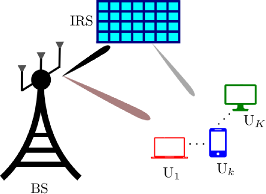
Figure 1: System model for IRS-assisted MU-MISO downlink.

III Proposed Solution

It is now clear that the non-convexity of (3b) is the main issue to address. In this section, we apply the SCA framework to tackle this problem by proposing a series of convex approximations. To this end, we recall the following inequality and equalities:

$$\|\mathbf{x}\|^{2} \ \geq 2\Re\{\mathbf{y}^{\mathsf{H}}\mathbf{x}\}-\|\mathbf{y}\|^{2},$$ (6a)

$$\Re\{\mathbf{x}^{\mathsf{H}}\mathbf{y}\} \ =\tfrac{1}{4}\big{(}\|\mathbf{x}+\mathbf{y}\|^{2}-\|\mathbf{x}-\mathbf{y}\|^{2}\big{)},$$ (6b)

$$\Im\{\mathbf{x}^{\mathsf{H}}\mathbf{y}\} \ =\tfrac{1}{4}\big{(}\|\mathbf{x}-j\mathbf{y}\|^{2}-\|\mathbf{x}+j\mathbf{y}\|^{2}\big{)},$$ (6c)

which hold for two arbitrary complex-valued vectors $\mathbf{x}$ and $\mathbf{y}$. Note that (6a) is obtained by linearizing $\|\mathbf{x}\|^{2}$ around $\mathbf{y}$ and the equality in (6a) occurs for $\mathbf{x}=\mathbf{y}$, and (6b) and (6c) are obtained by expanding the terms in the right hand side.

We deal with (3b) using the notion of SCA where both $\boldsymbol{\phi}$ and $\mathbf{w}$ are optimized in each iteration. First,  (3b) is equivalent to

$$\frac{|\mathbf{g}_{k}\mathbf{w}_{k}|^{2}}{\Gamma_{k}} \geq 1+\sum\nolimits_{l\in\mathcal{K}\setminus\{k\}}\big{(}t_{kl}^{2}+\bar{t}_{kl}^{2}\big{)},$$ (7a)

$$t_{kl} \geq|\Re\{\mathbf{g}_{k}\mathbf{w}_{l}\}|,\quad\forall l\in\mathcal{K}\setminus\{k\},$$ (7b)

$$\bar{t}_{kl} \geq\ |\Im\{\mathbf{g}_{k}\mathbf{w}_{l}\}|,\quad\forall l\in\mathcal{K}\setminus\{k\},$$ (7c)

where $t_{kl}$ and $\bar{t}_{kl}$ are newly introduced slack variables. It is straightforward to see that if (3b) is feasible, then so is (7) and vice versa.

Since the right-hand side (RHS) of (7a) is convex, we need to find a concave lower bound for the term $|\mathbf{g}_{k}\mathbf{w}_{k}|^{2}$ in (7a). Let $\boldsymbol{\phi}^{(n)}$ and $\mathbf{w}_{k}^{(n)}$ represent the value of $\boldsymbol{\phi}$ and $\mathbf{w}_{k}$ in the $n$-th iteration of the SCA process, respectively. Then we have

$$|\mathbf{g}_{k}\mathbf{w}_{k}|^{2}\overset{(\mathrm{a})}{\geq}\ 2\Re\big{\{}\big{(}a_{k}^{(n)}\big{)}^{\mathsf{H}}\mathbf{g}_{k}\mathbf{w}_{k}\big{\}}-\big{|}a_{k}^{(n)}\big{|}^{2}$$

$$\overset{(\mathrm{b})}{\geq}\ \tfrac{1}{2}\big{\{}\big{\|}\big{(}a_{k}^{(n)}\big{)}\mathbf{g}_{k}^{\mathsf{H}}+\mathbf{w}_{k}\big{\|}^{2}-\big{\|}\big{(}a_{k}^{(n)}\big{)}\mathbf{g}_{k}^{\mathsf{H}}-\mathbf{w}_{k}\big{\|}^{2}\big{\}}-\big{|}a_{k}^{(n)}\big{|}^{2}$$

$$\overset{(\mathrm{c})}{\geq}\ \Re\big{\{}\big{(}\mathbf{b}_{k}^{(n)}\big{)}^{\mathsf{H}}\big{[}\big{(}a_{k}^{(n)}\big{)}\mathbf{g}_{k}^{\mathsf{H}}+\mathbf{w}_{k}\big{]}\big{\}}-\tfrac{1}{2}\big{\|}\mathbf{b}_{k}^{(n)}\big{\|}^{2}$$

$$\qquad\qquad-\tfrac{1}{2}\big{\|}\big{(}a_{k}^{(n)}\big{)}\mathbf{g}_{k}^{\mathsf{H}}-\mathbf{w}_{k}\big{\|}^{2}-\big{|}a_{k}^{(n)}\big{|}^{2}$$

$$\triangleq\ f_{k}\big{(}\mathbf{w}_{k},\boldsymbol{\phi};\mathbf{w}_{k}^{(n)},\boldsymbol{\phi}^{(n)}\big{)},$$ (8)

where $a_{k}^{(n)}\triangleq\mathbf{g}_{k}^{(n)}\mathbf{w}_{k}^{(n)}$, $\mathbf{b}_{k}^{(n)}\triangleq a_{k}^{(n)}\big{(}\mathbf{g}_{k}^{(n)}\big{)}^{\mathsf{H}}+\mathbf{w}_{k}^{(n)}$, and $\mathbf{g}_{k}^{(n)}\triangleq\mathbf{h}_{\mathrm{t}k}+\mathbf{h}_{\mathrm{s}k}\operatorname{diag}(\boldsymbol{\phi}^{(n)})\mathbf{H}_{\mathrm{ts}}$. Specifically, $(\mathrm{a})$ and $(\mathrm{c})$ are due to (6a), and $(\mathrm{b})$ is due to (6b). It is easy to check that $f_{k}\big{(}\mathbf{w}_{k},\boldsymbol{\phi};\mathbf{w}_{k}^{(n)},\boldsymbol{\phi}^{(n)}\big{)}$ is jointly concave with respect to (w.r.t.) $\boldsymbol{\phi}$ and $\mathbf{w}$.

Using the fact that $u\geq|v|$ if and only if $u\geq v$ and $u\geq-v$, and using (6b) we can equivalently rewrite (7b) as

$$t_{kl}\geq\ \Re\{\mathbf{g}_{k}\mathbf{w}_{l}\}=\tfrac{1}{4}\big{(}\|\mathbf{g}_{k}^{\mathsf{H}}+\mathbf{w}_{l}\|^{2}-\|\mathbf{g}_{k}^{\mathsf{H}}-\mathbf{w}_{l}\|^{2}\big{)},$$ (9a)

$$t_{kl}\geq\ -\Re\{\mathbf{g}_{k}\mathbf{w}_{l}\}=\tfrac{1}{4}\big{(}\|\mathbf{g}_{k}^{\mathsf{H}}-\mathbf{w}_{l}\|^{2}-\|\mathbf{g}_{k}^{\mathsf{H}}+\mathbf{w}_{l}\|^{2}\big{)}.$$ (9b)

The non-convexity of (9a) is due to the negative quadratic term in the RHS. To convexify (9a), we apply (6a) with $\mathbf{x}=\mathbf{g}_{k}^{\mathsf{H}}-\mathbf{w}_{l}$ and $\mathbf{y}=\mathbf{g}_{k}^{(n)}-\big{(}\mathbf{w}_{l}^{(n)}\big{)}^{\mathsf{H}}$$-\|\mathbf{g}_{k}^{\mathsf{H}}-\mathbf{w}_{l}\|^{2}$, which yields

$$t_{kl}\geq\ \tfrac{1}{4}\big{[}\big{\|}\mathbf{g}_{k}^{\mathsf{H}}+\mathbf{w}_{l}\big{\|}^{2}-2\Re\big{\{}\big{(}\mathbf{g}_{k}^{(n)}-\big{(}\mathbf{w}_{l}^{(n)}\big{)}^{\mathsf{H}}\big{)}\big{(}\mathbf{g}_{k}^{\mathsf{H}}-\mathbf{w}_{l}\big{)}\big{\}}$$

$$\!\!\!\!\!+\big{\|}\big{(}\mathbf{g}_{k}^{(n)}\big{)}^{\mathsf{H}}\!-\!\mathbf{w}_{l}^{(n)}\big{\|}^{2}\big{]}\!\triangleq\!\mu_{kl}\big{(}\mathbf{w}_{l},\boldsymbol{\phi};\mathbf{w}_{l}^{(n)},\boldsymbol{\phi}^{(n)}\big{)}.$$ (10)

Note that the RHS in (10) is jointly convex w.r.t. $\boldsymbol{\phi}$ and $\mathbf{w}_{l}$, resulting in the convexity of $\mu_{kl}\big{(}\mathbf{w}_{l},\boldsymbol{\phi};\mathbf{w}_{l}^{(n)},\boldsymbol{\phi}^{(n)}\big{)}$. Following a similar line of arguments, we can approximate (9b) as

$$t_{kl}\geq\ \tfrac{1}{4}\big{[}\big{\|}\mathbf{g}_{k}^{\mathsf{H}}-\mathbf{w}_{l}\big{\|}^{2}-2\Re\big{\{}\big{(}\mathbf{g}_{k}^{(n)}+\big{(}\mathbf{w}_{l}^{(n)}\big{)}^{\mathsf{H}}\big{)}\big{(}\mathbf{g}_{k}^{\mathsf{H}}+\mathbf{w}_{l}\big{)}\big{\}}$$

$$\!\!\!\!\!+\big{\|}\big{(}\mathbf{g}_{k}^{(n)}\big{)}^{\mathsf{H}}\!+\!\mathbf{w}_{l}^{(n)}\big{\|}^{2}\big{]}\!\triangleq\!\hat{\mu}_{kl}\big{(}\mathbf{w}_{l},\boldsymbol{\phi};\mathbf{w}_{l}^{(n)},\boldsymbol{\phi}^{(n)}\big{)}.$$ (11)

Similarly, (7c) leads to the following two inequalities:

$$\bar{t}_{kl}\geq\ \Im\{\mathbf{g}_{k}\mathbf{w}_{l}\}=\tfrac{1}{4}\big{(}\big{\|}\mathbf{g}_{k}^{\mathsf{H}}-j\mathbf{w}_{l}\big{\|}^{2}-\big{\|}\mathbf{g}_{k}^{\mathsf{H}}+j\mathbf{w}_{l}\big{\|}^{2}\big{)},$$ (12a)

$$\bar{t}_{kl}\geq\ -\Im\{\mathbf{g}_{k}\mathbf{w}_{l}\}\!=\!\tfrac{1}{4}\big{(}\big{\|}\mathbf{g}_{k}^{\mathsf{H}}\!+\!j\mathbf{w}_{l}\big{\|}^{2}\!-\!\big{\|}\mathbf{g}_{k}^{\mathsf{H}}\!-\!j\mathbf{w}_{l}\big{\|}^{2}\big{)}.$$ (12b)

Using the same line of thought of (10), we can obtain a lower bound for (12) as follows:

$$\bar{t}_{kl}\geq\ \tfrac{1}{4}\big{[}\big{\|}\mathbf{g}_{k}^{\mathsf{H}}\!-\!j\mathbf{w}_{l}\big{\|}^{2}\!-\!2\Re\big{\{}\big{(}\mathbf{g}_{k}^{(n)}\!-\!j\big{(}\mathbf{w}_{l}^{(n)}\big{)}^{\mathsf{H}}\big{)}\big{(}\mathbf{g}_{k}^{\mathsf{H}}\!+\!j\mathbf{w}_{l}\big{)}\big{\}}$$

$$\!\!\!\!\!+\big{\|}\big{(}\mathbf{g}_{k}^{(n)}\big{)}^{\mathsf{H}}\!+\!j\mathbf{w}_{l}^{(n)}\big{\|}^{2}\big{]}\!\triangleq\!\nu_{kl}\big{(}\mathbf{w}_{l},\boldsymbol{\phi};\mathbf{w}_{l}^{(n)},\boldsymbol{\phi}^{(n)}\big{)},\!\!$$ (13)

$$\bar{t}_{kl}\geq\ \tfrac{1}{4}\big{[}\big{\|}\mathbf{g}_{k}^{\mathsf{H}}\!+\!j\mathbf{w}_{l}\big{\|}^{2}\!-\!2\Re\big{\{}\big{(}\mathbf{g}_{k}^{(n)}\!+\!j\big{(}\mathbf{w}_{l}^{(n)}\big{)}^{\mathsf{H}}\big{)}\big{(}\mathbf{g}_{k}^{\mathsf{H}}\!-\!j\mathbf{w}_{l}\big{)}\big{\}}$$

$$\!\!\!\!\!+\big{\|}\big{(}\mathbf{g}_{k}^{(n)}\big{)}^{\mathsf{H}}\!-\!j\mathbf{w}_{l}^{(n)}\big{\|}^{2}\big{]}\!\triangleq\!\hat{\nu}_{kl}\big{(}\mathbf{w}_{l},\boldsymbol{\phi};\mathbf{w}_{l}^{(n)},\boldsymbol{\phi}^{(n)}\big{)}.\!\!$$ (14)

1

2

Input: $\mathbf{w}^{(0)}$, $\boldsymbol{\phi}^{(0)}$, $\xi>0$

3

4$n\leftarrow 0$;

5

6repeat

7      

8      Solve  ($\mathcal{P}_{n+1}$) and denote the solution as $\mathbf{w}^{\star}$, $\boldsymbol{\phi}^{\star}$;

9      

10      Update: $\mathbf{w}^{(n+1)}\leftarrow\mathbf{w}_{k}^{\star}$, $\boldsymbol{\phi}^{(n+1)}\leftarrow\boldsymbol{\phi}^{\star}$;

11      

12      $n\leftarrow n+1$;

13      

14until convergence ;

Output: $\mathbf{w}^{\star}$, $\boldsymbol{\phi}^{\star}$

Algorithm 1 Proposed SCA-based Method to Solve (3).

We are left with the non-convexity of (3c). To avoid increasing the problem size, we tackle (3c) by first relaxing it to be an inequality (and thus convex) constraint, and then forcing the inequality to be an equality by adding a regularized term to the objective function in (3a), which results in the following optimization problem:

$$\underset{\mathbf{w},\boldsymbol{\phi}}{\operatorname{minimize}} \ \|\mathbf{w}\|^{2}-\xi\|\boldsymbol{\phi}\|^{2}$$ (15a)

$$\operatorname{subject~{}to} \ f_{k}\big{(}\mathbf{w}_{k},\boldsymbol{\phi};\mathbf{w}_{k}^{(n)},\boldsymbol{\phi}^{(n)}\big{)}$$

$$\quad\geq 1+\sum\nolimits_{l\in\mathcal{K}\setminus\{k\}}\big{(}t_{kl}^{2}+\bar{t}_{kl}^{2}\big{)},\forall k\in\mathcal{K},$$ (15b)

$$\ \eqref{eq:mukl},\eqref{eq:muBarkl},\eqref{eq:nukl},\eqref{eq:nuBarkl},\forall k,l\in\mathcal{K},k\neq l,$$ (15c)

$$\ |\phi_{n_{\mathrm{s}}}|\leq 1,\quad\forall n_{\mathrm{s}}\in\mathscr{N}_{\mathrm{s}},$$ (15d)

where $\xi>0$ is the regularization parameter. It can be shown that for sufficiently large $\xi$, (15d) is binding at the optimality when convergence is achieved for the problem in (15). Note that due to the concavity of the term $-\xi\|\boldsymbol{\phi}\|^{2}$, the objective in (15) is still non-convex. However, we can convexify (15a) using (6a). In summary, the approximate convex subproblem for (3) in the $(n\!+\!1)$-th iteration of the SCA process is given by

$$\underset{\mathbf{w},\boldsymbol{\phi},\mathbf{t},\bar{\mathbf{t}}}{\operatorname{minimize}} \ \|\mathbf{w}\|^{2}-\!\xi\big{[}2\Re\big{\{}\big{(}\boldsymbol{\phi}^{(n)}\big{)}^{\mathsf{H}}\boldsymbol{\phi}\big{\}}\!-\!\|\boldsymbol{\phi}^{(n)}\|^{2}\big{]} \mathcal{P}_{n+1}$$ ()

$$\operatorname{subject~{}to} \ \eqref{eq:SINR:final},\eqref{eq:groupedInequality},\eqref{eq:UMC-Relaxed},$$

where $\mathbf{t}=\{t_{kl}\}_{k,l\in\mathcal{K},k\neq l}$ and $\bar{\mathbf{t}}=\{\bar{t}_{kl}\}_{k,l\in\mathcal{K},k\neq l}$. Finally, the proposed SCA-based method for solving (3) is outlined in Algorithm 1. To obtain the initial points $(\mathbf{w}^{(0)},\boldsymbol{\phi}^{(0)})$ we randomly generate $\boldsymbol{\phi}^{(0)}$ and then find $\mathbf{w}^{(0)}$ by solving (4). We also note that ($\mathcal{P}_{n+1}$) is an SOCP problem, and can be solved efficiently using off-the-shelf solvers such as MOSEK [21].

III-A Convergence Analysis

Let $f(\mathbf{w},\boldsymbol{\phi})=\|\mathbf{w}\|^{2}-\xi\|\boldsymbol{\phi}\|^{2}$. For a given $\xi$, since the optimal solution of $(\mathcal{P}_{n})$ is also a feasible solution to $(\mathcal{P}_{n+1})$, Algorithm 1 yields a non-increasing objective sequence, i.e. $f(\mathbf{w}^{(n)},\boldsymbol{\phi}^{(n)})\geq f(\mathbf{w}^{(n+1)},\boldsymbol{\phi}^{(n+1)})$. Due to (15d), the objective sequence is bounded from below, i.e. $f(\mathbf{w},\boldsymbol{\phi})\geq-\xi N_{\mathrm{s}}$ and thus $f(\mathbf{w}^{(n)},\boldsymbol{\phi}^{(n)})$ is convergent. We can prove that the sequence of iterates is also convergent as follows. Let $\mathcal{X}^{(0)}=\{\mathbf{w},\boldsymbol{\phi}|f(\mathbf{w},\boldsymbol{\phi})\leq f(\mathbf{w}^{(0)},\boldsymbol{\phi}^{(0)})$ be the level set associated with the initial point. Note that $\mathcal{X}^{(0)}$ is closed. We further note that $f(\mathbf{w},\boldsymbol{\phi})\leq f(\mathbf{w}^{(0)},\boldsymbol{\phi}^{(0)})$ implies $\|\mathbf{w}\|^{2}\leq f(\mathbf{w}^{(0)},\boldsymbol{\phi}^{(0)})+\xi\|\boldsymbol{\phi}\|^{2}\leq f(\mathbf{w}^{(0)},\boldsymbol{\phi}^{(0)})+\xi N_{\mathrm{s}}$, meaning $\mathcal{X}^{(0)}$ is bounded and thus compact. Since the sequence $\{(\mathbf{w}^{(n)},\boldsymbol{\phi}^{(n)})\}$ must lie in the compact set $\mathcal{X}^{(0)}$, it has a limit point. We can prove that this limit point is a stationary point of the following problem

$$\underset{\mathbf{w},\boldsymbol{\phi}}{\operatorname{minimize}}\ \big{\{} \|\mathbf{w}\|^{2}-\xi\|\boldsymbol{\phi}\|^{2}\big{|}\eqref{eq:SINRC-Orig},\eqref{eq:UMC-Relaxed}\big{\}}.$$

If (15d) occurs with equality which holds for large $\xi$, then the limit point is also a stationary solution to (3). Interestingly, our numerical results show that this is always the case even for a small $\xi$. We remark that in the case (15d) is not satisfied when Algorithm 1 converges, we can simply scale $\boldsymbol{\phi}$ to satisfy (3c) and solve (4) to find the final solution.

III-B Complexity Analysis

Note that in ($\mathcal{P}_{n+1}$), we introduce a slack variable in the objective to replace the term $\|\mathbf{w}\|^{2}$. It is clear from ($\mathcal{P}_{n+1}$) that the size (in the real-domain) of the optimization variables is $2(KN_{\mathrm{t}}+N_{\mathrm{s}}+K(K-1))+1$, and the total number of SOC constraints is $K+4K(K-1)+N_{\mathrm{s}}+1$. Therefore, following [22, Sec. 6.6.2], the overall per-iteration complexity of the proposed SOCP-based algorithm is given by

$$\!\!\!\mathcal{C}_{\mathrm{SOCP}}=\mathcal{O}\big{[}2\big{(}4K^{2}+N_{\mathrm{s}}\big{)}^{0.5}\big{(}K^{2}+KN_{\mathrm{t}}+N_{\mathrm{s}}\big{)}\big{(}4K^{5}$$

$$\!\!\!\!\!+16K^{3}N_{\mathrm{t}}+8K^{2}N_{\mathrm{s}}+20K^{2}N_{\mathrm{t}}^{2}+8KN_{\mathrm{t}}N_{\mathrm{s}}+4N_{\mathrm{s}}^{2})\big{]}.$$ (16)

In practice, an IRS usually has a large number of reflecting elements, i.e., $N_{\mathrm{s}}\gg\max\{N_{\mathrm{t}},K\}$ [23, 24]. Therefore, using (16), the approximate per-iteration complexity of the proposed SOCP-based algorithm is given by $\mathcal{C}_{\mathrm{SOCP}}\approx\text{$\mathcal{O}\big{(}N_{\mathrm{s}}^{0.5}\times N_{\mathrm{s}}\times N_{\mathrm{s}}^{2}\big{)}$}=\mathcal{O}\big{(}N_{\mathrm{s}}^{3.5}\big{)}$. On the other hand, since the complexity of [11, Algorithm 1] is dominated by that of solving (5) using SDP, the per-iteration complexity of the SDR-based algorithm in [11, Algorithm 1] is given by $\mathcal{C}_{\mathrm{SDR}}\approx\mathcal{O}\big{(}N_{\mathrm{s}}^{7}\big{)}$ [22, Sec. 6.6.2], which is significantly higher than that of our proposed algorithm. This will be numerically shown in the next section.

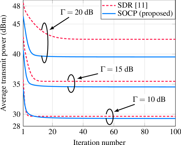
Figure 2: Convergence results for $N_{\mathrm{t}}=K=4$ and $N_{\mathrm{s}}=100$.

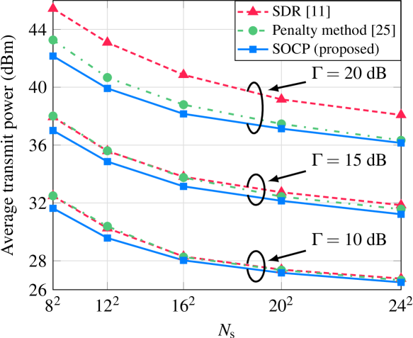
Figure 3: Average transmit power versus $N_{\mathrm{s}}$ for $N_{\mathrm{t}}=K=6$.

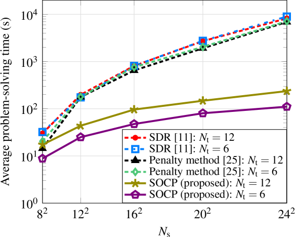
Figure 4: Average problem solving time versus $N_{\mathrm{s}}$ for $K=6$ and $\Gamma=10$ dB.

III-C Application of the Proposed Method to Other Problems

We remark that the proposed solution is dedicated to ($\mathcal{P}_{n+1}$), but it has wider applicability. We now provide a brief discussion on how the proposed solution can be applied to other IRS-related design problems with slight modifications. The problem (10) in [7] has exactly the same constraints as (3b) and (3c), and thus the proposed SOCP-based approach can directly be applied. Also, the non-convex constraints of the PowerMin problem in [8] are the same as (3b) and (3c), and thus Algorithm 1 is still directly applicable. Following a similar line of arguments, one can easily see that the proposed algorithm can be slightly modified to solve [9, (P1)] and [10, (P1)], among the others.

IV Numerical Results and Discussion

We assume that the system operates at the center frequency of 2 GHz with a total available bandwidth of 20 MHz. It is assumed that the center of the BS uniform linear array and the center of the IRS uniform planar array are located at $(0\ \mathrm{m},20\ \mathrm{m},10\ \mathrm{m})$ and $(30\ \mathrm{m},0\ \mathrm{m},5\ \mathrm{m})$, respectively. The distance between the neighboring antennas at the BS, as well as that between the neighboring elements at the IRS is equal to $\lambda/2$, where $\lambda$ is the wavelength of the carrier waves. The single-antenna users are assumed to be randomly distributed inside a circular disk of radius $5\ \mathrm{m}$, centered at $(350\ \mathrm{m},10\ \mathrm{m},2\ \mathrm{m})$, ensuring that the minimum distance between the users is equal to $2\lambda$. We model the Rician distributed small-scale fading and distance-dependent path loss for all of the wireless links according to [15, Sec. VI]. The noise spectral density at each of the user node is assumed to equal to -174dBm/Hz. Without loss of generality, it is assumed that $\Gamma_{k}=\Gamma,\ \forall k\in\mathcal{K}$ and $\xi=0.001$. In Figs. 2–4, the averaging is performed over 100 independent small-scale channel fading realizations, and we consider 1000 independent vectors for Gaussian randomization in each iteration for the SDR-based baseline algorithm. The simulations are performed on a Linux PC with 7.5 GiB memory and Intel Core i5-7200U CPU, using Python v3.9.7 and MOSEK Fusion API for Python Rel.-9.2.49 [21]. It is noteworthy that when the value of the target SINR $\Gamma$ is small, the SINR constraints can be met easily. In such a scenario, the impact of the SINR constraints on the optimization problem is minimal, and therefore, different optimization schemes may achieve similar performance. Therefore, we consider high/stricter SINR requirements in our simulations.

Fig. 2 shows the convergence comparison of the proposed SOCP- and SDR-based [11] algorithms. It is evident from the figure that Algorithm 1 outperforms the SDR-based algorithm in terms of required transmit power. More interestingly, as the QoS constraints becomes more demanding (i.e., for large $\Gamma$), the performance gap between the two algorithms increases. For large values of $\Gamma$, in fact, the likelihood of obtaining a suitable Gaussian vector via randomization that satisfies the QoS constraints decreases, resulting in the inferior performance of SDR-based algorithm. In the remaining experiments, we stop Algorithm 1 and the SDR-based method when either the relative change in the objective is less than $10^{-5}$ or the number of iterations is 20.

The impact of $N_{\mathrm{s}}$ on the average transmit power is shown in Fig. 3. In this figure, we also show the performance of a penalty-based AO method [25], which can be modified to solve the PowerMin problem. As expected, the average transmit power to maintain the desired QoS decreases as $N_{\mathrm{s}}$ is increased. For large values of $N_{\mathrm{s}}$, in fact, the IRS performs a highly-focused beamforming to achieve the desired QoS even for small values of the transmit power. It is evident from the figure that the SDR-based and penalty-based methods perform quite similarly for small values of $\Gamma$. For large $\Gamma$, however, the coupling among the optimization variables becomes stronger, resulting in better performance for the penalty-based method compared to the SDR-based method. Since all the design variables are updated simultaneously, the SOCP-based method outperforms both the SDR- and penalty-based methods relying on AO.

In Fig. 4, we show the average problem-solving-time comparison between the proposed SOCP-based and SDR-based algorithms. As expected, the required run-time increases with increasing values of $N_{\mathrm{s}}$ for both the algorithms. Also, in line with the complexity analysis in Section III-B, the run-time for the SDR-based algorithm is much larger than that for the proposed SOCP-based algorithm. Finally, we note that the per-iteration complexity of the method in [25] is $\mathcal{O}(N_{\mathrm{s}}^{3})$, which is slightly less than $\mathcal{O}(N_{\mathrm{s}}^{3.5})$ provided by our proposed method. However, the method in [25] needs a significantly larger number of iterations to converge (compared to the SOCP- and SDR-based methods). Compared to the proposed SOCP-based method, thus, it takes a much larger overall run time to return a solution, as shown in Fig. 4.

V Conclusion

We have presented the joint transmit beamforming and IRS phase-shift design to minimize the transmit power in an IRS-assisted MU-MIMO downlink communication system with QoS constraints. Specifically, we proposed an SCA-assisted SOCP framework for solving the PowerMin problem where all of the optimization variables are updated in each iteration, simultaneously, in contrast to the conventional SDR- and penalty-based algorithms in which only one set of optimization variables is updated in each iteration with the others being fixed. The proposed algorithm was shown to outperform the state-of-the-art benchmark schemes in terms of both the required transmit power and the computational complexity/average problem-solving time, and is promising to be applied to solve other similar design problems in IRS-aided communications.

References

- [1] H. Yang et al., “A programmable metasurface with dynamic polarization, scattering and focusing control,” Scientific reports, vol. 6, no. 1, pp. 1–11, 2016.
- [2] M. Di Renzo et al., “Smart radio environments empowered by reconfigurable intelligent surfaces: How it works, state of research, and the road ahead,” IEEE J. Sel. Areas Commun., vol. 38, no. 11, pp. 2450–2525, 2020.
- [3] C. Pan et al., “Reconfigurable intelligent surfaces for 6G systems: Principles, applications, and research directions,” IEEE Commun. Mag., vol. 59, no. 6, pp. 14–20, 2021.
- [4] Q. Wu, S. Zhang, B. Zheng, C. You, and R. Zhang, “Intelligent reflecting surface-aided wireless communications: A tutorial,” IEEE Trans. Commun., vol. 69, no. 5, pp. 3313–3351, 2021.
- [5] W. Mei, B. Zheng, C. You, and R. Zhang, “Intelligent reflecting surface-aided wireless networks: From single-reflection to multireflection design and optimization,” Proc. IEEE, pp. 1–21, to appear.
- [6] Q. Wu and R. Zhang, “Towards smart and reconfigurable environment: Intelligent reflecting surface aided wireless network,” IEEE Commun. Mag., vol. 58, no. 1, pp. 106–112, 2020.
- [7] Z. Yang, W. Xu, C. Huang, J. Shi, and M. Shikh-Bahaei, “Beamforming design for multiuser transmission through reconfigurable intelligent surface,” IEEE Trans. Commun., vol. 69, no. 1, pp. 589–601, 2021.
- [8] Y. Liu, J. Zhao, M. Li, and Q. Wu, “Intelligent reflecting surface aided MISO uplink communication network: Feasibility and power minimization for perfect and imperfect CSI,” IEEE Trans. Commun., vol. 69, no. 3, pp. 1975–1989, 2021.
- [9] J. Wu and B. Shim, “Power minimization of intelligent reflecting surface-aided uplink IoT networks,” in IEEE WCNC, 2021, pp. 1–6.
- [10] H. Han et al., “Reconfigurable intelligent surface aided power control for physical-layer broadcasting,” IEEE Trans. Commun., vol. 69, no. 11, pp. 7821–7836, 2021.
- [11] Q. Wu and R. Zhang, “Intelligent reflecting surface enhanced wireless network via joint active and passive beamforming,” IEEE Trans. Wireless Commun., vol. 18, no. 11, pp. 5394–5409, 2019.
- [12] R. Liu, M. Li, Q. Liu, and A. L. Swindlehurst, “Joint symbol-level precoding and reflecting designs for IRS-enhanced MU-MISO systems,” IEEE Trans. Wireless Commun., vol. 20, no. 2, pp. 798–811, 2021.
- [13] B. Guo, R. Li, and M. Tao, “Joint design of hybrid beamforming and phase shifts in RIS-aided mmWave communication systems,” in IEEE WCNC, 2021, pp. 1–6.
- [14] Q. Wu and R. Zhang, “Joint active and passive beamforming optimization for intelligent reflecting surface assisted SWIPT under QoS constraints,” IEEE J. Sel. Areas Commun., vol. 38, no. 8, pp. 1735–1748, 2020.
- [15] N. S. Perović, L.-N. Tran, M. Di Renzo, and M. F. Flanagan, “On the maximum achievable sum-rate of the RIS-aided MIMO broadcast channel,” arXiv preprint arXiv:2110.01700, 2021.
- [16] V. Kumar, M. Flanagan, R. Zhang, and L.-N. Tran, “Achievable rate maximization for underlay spectrum sharing MIMO system with intelligent reflecting surface,” IEEE Wireless Commun. Lett., vol. 11, no. 8, pp. 1758–1762, 2022.
- [17] C. Pan et al., “An overview of signal processing techniques for RIS/IRS-aided wireless systems,” IEEE J. Sel. Topics Signal Process., pp. 1–35, to appear.
- [18] B. Zheng, C. You, W. Mei, and R. Zhang, “A survey on channel estimation and practical passive beamforming design for intelligent reflecting surface aided wireless communications,” IEEE Commun. Surveys Tuts., vol. 24, no. 2, pp. 1035–1071, 2022.
- [19] N. Sidiropoulos, T. Davidson, and Z.-Q. Luo, “Transmit beamforming for physical-layer multicasting,” IEEE Trans. Signal Process., vol. 54, no. 6, pp. 2239–2251, 2006.
- [20] M. Bengtsson and B. Ottersten, “Optimum and suboptimum transmit beamforming,” in Handbook of antennas in wireless communications. CRC press, 2018, pp. 18–1.
- [21] MOSEK ApS, MOSEK Fusion API for Python. Release 9.2.49, 2021. [Online]. Available: http://docs.mosek.com/9.2/pythonfusion.pdf
- [22] A. Ben-Tal and A. Nemirovski, Lectures on modern convex optimization. Philadelphia: SIAM, 2011.
- [23] L. Dai et al., “Reconfigurable intelligent surface-based wireless communications: Antenna design, prototyping, and experimental results,” IEEE Access, vol. 8, pp. 45 913–45 923, 2020.
- [24] X. Pei et al., “RIS-aided wireless communications: Prototyping, adaptive beamforming, and indoor/outdoor field trials,” IEEE Trans. Commun., vol. 69, no. 12, pp. 8627–8640, 2021.
- [25] M. Hua, Q. Wu, W. Chen, O. A. Dobre, and A. L. Swindlehurst, “Secure intelligent reflecting surface aided integrated sensing and communication,” arXiv preprint arXiv:2207.09095, 2022.