Catastrophic Cooling in Superwinds. III. Non-equilibrium Photoionization

Abstract

Observations of some starburst-driven galactic superwinds suggest that strong radiative cooling could play a key role in the nature of feedback and the formation of stars and molecular gas in star-forming galaxies. These catastrophically cooling superwinds are not adequately described by adiabatic fluid models, but they can be reproduced by incorporating non-equilibrium radiative cooling functions into the fluid model. In this work, we have employed the atomic and cooling module maihem implemented in the framework of the flash hydrodynamics code to simulate the formation of radiatively cooling superwinds as well as their corresponding non-equilibrium ionization (NEI) states for various outflow parameters, gas metallicities, and ambient densities. We employ the photoionization program cloudy to predict radiation- and density-bounded photoionization for these radiatively cooling superwinds, and we predict UV and optical line emission. Our non-equilibrium photoionization models built with the NEI states demonstrate the enhancement of C iv, especially in metal-rich, catastrophically cooling outflows, and O vi in metal-poor ones.

]Received 2022 June 1; revised 2022 July 30; accepted 2022 August 3

1 Introduction

Observations of star-forming galaxies reveal the presence of galactic outflows, known as superwinds (Heckman et al., 1990), with multiphase structures having regions with low temperatures ($10^{1{\rm-}3}$ K) based on sub-millimeter and infrared observations (Ott et al., 2005b; Weiß et al., 2005; Bolatto et al., 2013; Leroy et al., 2015), warm ($\approx 10^{4{\rm-}4.5}$ K) wind regions as seen in optical and near-UV measurements (Walsh & Roy, 1989; Izotov & Thuan, 1999; James et al., 2009, 2013), as well as hot ($10^{6.5{\rm-}8}$ K) bubbles in X-ray observations (della Ceca et al., 1996; Strickland et al., 1997; Martin, 1999; Ott et al., 2005a). Historically, starburst-driven superwinds have been modeled using adiabatic assumptions (Castor et al., 1975; Weaver et al., 1977; Chevalier & Clegg, 1985; Cantó et al., 2000). However, adiabatic models are not consistent with suppressed superwinds observed in several starburst galaxies such as M82 (Smith et al., 2006; Westmoquette et al., 2014), NGC 5253 (Turner et al., 2017), NGC 2366 (Oey et al., 2017), and extreme Green Peas (GPs; Jaskot et al., 2017). In particular, cooling superwinds can produce virial temperatures below $10^{4}$ K, and can stimulate star formation (Fabian et al., 1984; Sarazin, 1988; Krause et al., 2016; Silich & Tenorio-Tagle, 2017) and extensive molecular gas (e.g., Veilleux et al., 2020).

Semianalytic solutions for radiative superwinds, which have been obtained with cooling functions (e.g., Silich et al., 2003, 2004; Tenorio-Tagle et al., 2005, 2007), show that temperature profiles of superwinds have significant departures from the adiabatic solutions, and are therefore also known as catastrophic cooling models. These semi-analytical results indicate that radiative cooling is contingent on the gas metallicity, mass loading, and kinetic heating efficiency. A semi-analytic analysis of such a model by Wünsch et al. (2011) also demonstrates that strong radiative cooling with low heating efficiency is more sensitive to the gas metallicity, while the metallicity effect is not significant with large mass loading. More recently, hydrodynamic simulations of superwinds have also been carried out by Danehkar et al. (2021), which confirmed the parametric dependence of radiative cooling. Photoionization calculations have been conducted by Danehkar et al. (2021) under the assumption that gas is in collisional ionization equilibrium (CIE) and photoionization equilibrium (PIE). The radiative cooling functions have been calculated in CIE by a number of authors (Cox & Tucker, 1969; Raymond et al., 1976; Shull & van Steenberg, 1982; Sutherland & Dopita, 1993; Bryans et al., 2006). The cooling functions for gas in ionization equilibrium have been employed for modeling radiatively cooling superwinds (see e.g. Schneider et al., 2018; Lochhaas et al., 2018, 2020). However, the CIE assumption is not entirely correct when the time-scale of ionization or recombination of a gas exceeds its cooling time (Gnat & Sternberg, 2007; Oppenheimer & Schaye, 2013).

Time-dependent radiative cooling functions produce non-equilibrium ionization (NEI) states that have significant departures from CIE states (Kafatos, 1973; Shapiro & Moore, 1976; Schmutzler & Tscharnuter, 1993; Gnat & Sternberg, 2007; Vasiliev, 2011; Oppenheimer & Schaye, 2013). At temperatures below $10^{6}$ K, where the gas is transiting from pure CIE to PIE, NEI departures from CIE are predicted to be considerable (Vasiliev, 2011). A non-equilibrium chemistry network with cooling functions was incorporated into a module called maihem (Gray et al., 2015; Gray & Scannapieco, 2016) for hydrodynamic simulations with flash. The formation of radiatively cooling superwinds and their emission lines has been investigated using maihem (Gray et al., 2019a, hereafter Paper I). In Danehkar et al. (2021, hereafter Paper II), we explored the parameter space for radiatively cooling superwinds using a grid of hydrodynamic simulations from maihem, made in the parameter space of the metallicity ($Z$), mass loading ($\dot{M}$), wind velocity ($V_{\infty}$), and ambient density ($n_{\rm amb}$), finding that cooling is enhanced by increasing the gas metallicity and mass-loading rate, and decreasing the wind velocity. We employed the physical conditions produced by our hydrodynamic simulations to create a grid of collisional ionization and photoionization (CPI) models, also predicting UV and optical emission lines under CIE conditions.

Paper I indicates that NEI states can generate enhanced emission from highly ionized UV lines such as O vi and C iv. Therefore, in the present work, we additionally incorporate NEI states predicted by maihem into non-equilibrium photoionization (NPI) models in the same parameter space grid considered in Paper II, which allows us to investigate the implications of NEI calculations for catastrophically cooling superwinds. In Section 2, we briefly describe our maihem hydrodynamic settings and results. In Section 3, we explain how we build NPI modeling with NEI states generated by maihem. UV emission lines produced by cloudy and diagnostics diagrams are explained in Section 4. Applications of NPI models for observations are discussed in Section 5, followed by a summary and conclusions in Section 6.

2 Hydrodynamic Simulations

A complete description of the maihem code and our adopted parameters is given in Paper II. Here, we provide a brief summary.

We use a directionally unsplit hydrodynamic solver (Lee et al., 2009; Lee & Deane, 2009; Lee, 2013) with a hybrid Riemann solver (Toro et al., 1994) and a second-order MUSCL–Hancock reconstruction scheme (van Leer, 1979) in the framework of the adaptive mesh hydrodynamics code flash v4.5 (Fryxell et al., 2000) to solve the continuity equation, Euler equation, and energy conservation equation of the fluid model of superwinds with negligible gravitational forces in one-dimensional spherical coordinates that are coupled to the radiative cooling and photo-heating functions of the maihem package:

$$\frac{d\rho_{w}}{dt}+\frac{1}{r^{2}}\frac{d}{dr}\left(\rho_{w}u_{w}r^{2}\right) =q_{m},$$ (1)

$$\rho_{w}\frac{du_{w}}{dt}+\rho_{w}u_{w}\frac{du_{w}}{dr}+\frac{dP_{w}}{dr} =-q_{m}u_{w},$$ (2)

$$\rho_{w}\frac{d{E}_{w}}{dt}+\frac{1}{r^{2}}\frac{d}{dr}\bigg{[}\rho_{w}u_{w}r^{2}\bigg{(}\frac{u_{w}^{2}}{2}+ \frac{\gamma}{\gamma-1}\frac{P_{w}}{\rho_{w}}\bigg{)}\bigg{]}$$

$$=q_{e}-q_{c}+q_{h},$$ (3)

where $\rho_{w}$ is the fluid density, ${u}_{w}$ the fluid velocity, $P_{w}=\left(\gamma-1\right)\rho_{w}\epsilon_{w}$ the thermal pressure with an ideal gas equation of state, ${E}_{w}=\epsilon_{w}+\frac{1}{2}\left|u_{w}\right|^{2}$ the total energy per unit mass, $\epsilon_{w}$ the internal energy per unit mass, $\gamma=5/3$ the ratio of specific heats, $q_{m}=\dot{M}_{\rm sc}/V_{\rm sc}$ the mass deposition rate per unit volume, $q_{e}=\dot{E}_{\rm sc}/V_{\rm sc}$ the energy deposition rate per unit volume, $\dot{M}_{\rm sc}$ the mass-loading rate, $\dot{E}_{\rm sc}$ the energy deposition rate, $V_{\rm sc}=\frac{4}{3}\pi R^{3}_{\rm sc}$ the SSC volume, $R_{\rm sc}$ the cluster radius, $q_{c}$ the radiative cooling rates per unit volume, and $q_{h}$ the photo-heating rate per unit volume. In a steady state ($d/dt=0$), the fluid equations take the forms presented in Paper II that were semianalytically studied by Silich et al. (2004). Outside the SSC ($r>R_{\rm sc}$), $q_{m}=0$ and $q_{e}=0$, while $q_{c}$ and $q_{h}$ also vanish inside the SSC ($r<R_{\rm sc}$) with negligible radiative effects. The steady-state fluid equations reduce to the adiabatic solutions obtained by Chevalier & Clegg (1985) and Cantó et al. (2000) in the absence of the radiative functions $q_{c}$ and $q_{h}$.

As fully described in Paper II, we set the boundary conditions for the density, temperature, and velocity of the outflow at the cluster boundary ($r=R_{\rm sc}$) according to the semianalytic solutions (Chevalier & Clegg, 1985; Cantó et al., 2000; Silich et al., 2004) as follows:

$$\begin{array}[c]{ccc}\rho_{w}=\dfrac{\dot{M}_{\rm sc}}{2\pi R_{\rm sc}^{2}V_{\infty}},{}{}{}{}&T_{w}=\dfrac{1}{4\gamma}\dfrac{\mu_{\rm p}}{k_{\rm B}}V_{\infty}^{2},~{}~{}~{}~{}u_{w}=\dfrac{1}{2}V_{\infty},\end{array}$$ (4)

where $V_{\infty}=(2\dot{E}_{\rm sc}/\dot{M}_{\rm sc})^{1/2}$ is the actual wind velocity, $\mu_{\rm p}=\mu m_{\rm p}$ the mean mass per particle, $\mu\approx 0.61$ the mean atomic weight of particles for a fully ionized gas in units of the proton mass $m_{\rm p}$, and $k_{\rm B}$ the Boltzmann constant. We also set the initial conditions ($t=0$) of the density, temperature, and velocity of the ambient medium outside the SSC ($r>R_{\rm sc}$) as $\rho_{w}=\mu_{\rm p}n_{\rm amb}$, $T_{w}=T_{\rm amb}$, and $u_{w}=0$, where $n_{\rm amb}$ is the number density of the ambient medium, and $T_{\rm amb}$ is the ambient temperature that is calculated in PIE by cloudy for the density profile predicted by an initial maihem run with $T_{\rm amb}=10^{3}$ K.

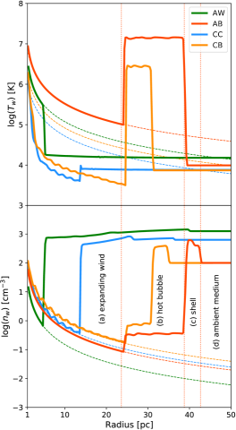
Figure 1: Top Panel: Wind classification modes based on various temperature profiles, namely the adiabatic wind (AW), adiabatic bubble (AB), catastrophic cooling (CC), and catastrophic cooling bubble (CB), as defined by Danehkar et al. (2021). Temperature profiles (solid lines) are plotted along with their adiabatic predictions (dashed lines). Bottom Panel: The different regions for the AB wind mode are labeled on the density profile and separated by dotted lines: (a) expanding wind, (b) hot bubble, (c) shell, and (d) ambient medium. Density profiles (solid lines) are plotted along with their adiabatic solutions (dashed lines).

The radiative cooling rate $q_{c}$ and photo-heating rate $q_{h}$ per volume are calculated by the maihem module (Gray et al., 2019b) using the ion-by-ion cooling efficiencies $\Lambda_{i}$, the photo-heating efficiencies $\Gamma_{i}$, the number densities $n_{i}$ of ionic species $i$, and the number density of electrons $n_{e}$:

$$\begin{array}[c]{cc}q_{c}=\displaystyle\sum_{i}n_{i}n_{e}\Lambda_{i},{}{}{}{}&q_{h}=\displaystyle\sum_{i}n_{i}\Gamma_{i},\end{array}$$ (5)

where the cooling efficiencies $\Lambda_{i}$ are calculated for a given wind temperature $T_{w}$ through interpolation on the ion-by-ion cooling rates from Gnat & Ferland (2012) that are also extended down to 5000 K by Gray et al. (2015), and the photo-heating efficiencies $\Gamma_{i}=\int^{\infty}_{\nu_{0,i}}(4\pi J_{\nu}/h\nu)h(\nu-\nu_{0,i})\sigma_{i}(\nu){\rm d}\nu$ ($\nu$ frequency, $\nu_{0,i}$ ionization frequency, and $h$ the Planck constant) are calculated for a given ionizing spectral energy distribution (SED) $J_{\nu}$ using the photoionization cross sections $\sigma_{i}(\nu)$ from Verner & Yakovlev (1995) and Verner et al. (1996) as implemented by Gray & Scannapieco (2016) and expanded for further ions in the species network of Gray et al. (2019b). The maihem module for photo-heating calculations is supplied with the ionizing SED made by Starburst99 (Leitherer et al., 1999, 2014) for the fiducial model at age 1 Myr with total stellar mass of $M_{\star}=2.05\times 10^{6}$ M_⊙ and metallicity close to the gas metallicity $Z$.

We produce a grid of hydrodynamic simulations in the parameter space of the metallicity $Z$, mass loading $\dot{M}_{\rm sc}$, wind velocity $V_{\infty}$, and ambient density $n_{\rm amb}$. We consider the gas metallicity of $\hat{Z}\equiv Z/$Z${}_{\odot}=1$, $0.5$, $0.25$, and $0.125$, where $Z/$Z${}_{\odot}=1$ associated with the baseline ISM abundances given in Table 2 of Paper II, the mass-loading rate $\dot{M}_{\rm sc}=10^{-1}$, $10^{-2}$, $10^{-3}$, and $10^{-4}\times\hat{Z}^{0.72}$ M_⊙ yr^-1 according to $\dot{M}_{\rm sc}\varpropto Z^{0.72}$ (Mokiem et al., 2007), the wind terminal speed $V_{\infty}=250$, $500$, and $1000\times\hat{Z}^{0.13}$ km s^-1 according to $V_{\infty}\varpropto Z^{0.13}$ (Vink et al., 2001), and the ambient density $n_{\rm amb}=1$, $10$, $10^{2}$, and $10^{3}$ cm^-3. The C/O ratio is also parameterized by the metallicity (described by Danehkar et al., 2021). The resulting density and temperature profiles for various parameters are shown as an interactive figure and animation in Figures 2 and 3 of Paper II.

In Paper II, we classified our simulated superwinds according to adiabatic/radiative cooling and the presence/absence of the hot bubble, namely: the adiabatic wind (AW), adiabatic bubble (AB), catastrophic cooling (CC), and catastrophic cooling bubble (CB). Temperature and density profiles of one example of each of the four wind classification modes are plotted in Figure 1. Moreover, we assigned the adiabatic, pressure-confined (AP) and cooling, pressure-confined (CP) wind modes to those models whose bubble expansions are stalled by thermal pressures from the ambient media (see animation in Figure 3 of Paper II). While models with adiabatic and radiative cooling (AW and CC) thereby suppress the hot bubble, there are many models with strong radiative cooling that still do have a bubble (CB). Two fully suppressed wind modes were also defined, namely no wind (NW) and momentum-conserving (MC) evolution. In the NW mode, the wind is completely inhibited where the supersonic outflow pressure analytically found by Cantó et al. (2000) is less than the ambient pressure. In the MC mode, radiative cooling caused by high mass deposition and low heating efficiency is able to completely suppress the wind before it is launched. The wind classification in the parameter space shown in Figure 4 of Paper II indicates that radiative cooling is enhanced by an increase in $\dot{M}_{\rm sc}$ and $Z$, and a decrease in $V_{\infty}$.

Our hydrodynamic simulations have been conducted without the gravity module. In particular, the Jeans length of the ionized ambient medium with density $10^{3}$ cm^-3 and temperature $10^{4}$ K (corresponding to the sound speed $\approx 15$ km s^-1), is approximately equal to 100 pc, which could be comparable to the size of the H ii region. Thermal pressure cannot resist gravitational collapse on scales larger than the Jeans length, while the self-gravity is negligible below it. A gravitational collapse occurs in cool clouds of high density formed by radiative cooling superwinds, which leads to star formation. Detailed handling of self-gravity and optical depth for the ambient diffuse radiation is computationally expensive (see e.g. Truelove et al., 1997; Wünsch et al., 2018, 2021) and is beyond the scope of this work.

3 Non-equilibrium Photoionization Modeling

We conduct non-equilibrium photoionization modeling for the physical conditions ($T_{w}$ and $n_{w}$) and NEI states produced by our maihem simulations using cloudy v17.02 (Ferland et al., 1998, 2013, 2017). The SED and ionizing luminosity of the SSC calculated by Starburst99 are provided as inputs into our cloudy models to specify an ionizing source (the same as Paper II). Non-equilibrium calculations are now made using the outflow temperature $T_{w}$, outflow density $n_{w}$ and time-dependent NEI states obtained as a function of the radius $r$ derived from our maihem simulations. In Paper II, we generated PI models based on the Starburst99 SEDs using only $n_{w}$, and CPI models with $T_{w}$ and $n_{w}$ produced by maihem without the use of NEI states.

Time-dependent calculations of the NEI states are performed by maihem using the atomic data for recombination, collisional ionization, and photoionization. In non-equilibrium conditions, the number density of each ion $n_{i}$ of each chemical element $A$ evolves according to the time-dependent ionization balance equation (see e.g. Dopita & Sutherland, 2003):

$$\frac{dn_{A,i}}{dt}= n_{\rm e}n_{A,i+1}\alpha^{A,i+1}_{\rm rec}-n_{\rm e}n_{A,i}\alpha^{a,i}_{\rm rec}$$

$$+n_{\rm e}n_{A,i-1}R^{A,i-1}_{\rm coll}-n_{\rm e}n_{A,i}R^{A,i}_{\rm coll}$$

$$+n_{A,i-1}\zeta^{A,i-1}_{\rm phot}-n_{A,i}\zeta^{A,i}_{\rm phot},$$ (6)

where $\alpha^{A,i}_{\rm rec}$ is the recombination coefficient of the ion ${i}$ of element $A$, including the radiative recombination rate (Badnell, 2006) and dielectronic recombination rate (see Table 1 in Gray et al., 2015), $R^{A,i}_{\rm coll}$ is the collisional ionization rate from Voronov (1997), $\zeta^{i,A}_{\rm phot}=\int^{\infty}_{\nu_{0,i}}(4\pi J_{\nu}/h\nu)\sigma_{i,A}(\nu){\rm d}\nu$ is the photoionization rate of each ion determined from the specified SED field $J_{\nu}$ and the photoionization cross-section $\sigma_{i,A}(\nu)$ (Verner & Yakovlev, 1995; Verner et al., 1996).

Non-equilibrium ionization occurs in regions where the radiative cooling timescale $\tau_{\rm cool}\approx 3k_{\rm B}T_{w}/(n_{\rm e}\Lambda)$ is shorter than the collisional ionization timescale $\tau_{\rm CIE}\approx 1/(n_{\rm e}\alpha^{A,i}_{\rm rec}+n_{\rm e}R^{A,i}_{\rm coll})$, where $\Lambda$ is the total radiative cooling efficiency. In the expanding wind region, where density is low ($\lesssim 1$ cm^-3), this condition where $\tau_{\rm cool}<\tau_{\rm CIE}$ is obtained for C iv and O vi at temperatures below $10^{6}$ K. Thus, these ions may be in NEI states because of radiative cooling, while most ions still remain in CIE $(\tau_{\rm cool}\gg\tau_{\rm CIE}$). Figure 2 shows the radiative cooling timescale and the collisional ionization timescales of different C ions (top panel) and O ions (bottom) plotted against the electron temperature. We calculated the radiative cooling timescale using the total cooling efficiency from Gnat & Ferland (2012), and the CIE timescales using the atomic data for recombination and collisional ionization. The figure compares the timescales for $n_{\rm e}=1$ cm^-3 and the solar composition. It can be seen that the ionization timescales of C v, C iv, and O vi are longer than the radiative cooling timescale at temperatures below $10^{6}$ K, where these ions are in NEI conditions.

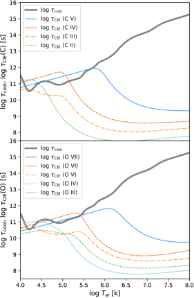
Figure 2: The collisional ionization timescales ($\tau_{\rm CIE}$) for ionic species of carbon (top panel) and oxygen (bottom), along with the radiative cooling timescale ($\tau_{\rm cool}$), as a function of the gas temperature ($T_{w}$) for a plasma with $n_{\rm e}=1$ cm^-3 and the solar abundances.

To build the NPI models, the density and temperature structures of the outflow extracted from our maihem simulations are employed to calculate emissivities by performing cloudy runs for all individual zones. The NEI states computed by maihem with SED are also supplied as inputs to cloudy. The ionizing SED and luminosity produced by Starburst99 are provided in our cloudy model to include combined photoionization and non-equilibrium ionization, decreasing the luminosity by distance from the SSC as $r^{-2}$. Following Paper II, the results predicted by the CPI model are applied to the ambient medium for the ionized, isothermal part of the shell starting outward from $\sim 1$–2 pc after the interior boundary of the shell. The final emissivity profiles of emission lines are built by combining the NEI results of all the outflow zones and the CPI results of the ambient medium. The NPI model for the outflow region is therefore created by zone-by-zone cloudy calculations based on NEI states generated by maihem that requires an individual cloudy run for each zone. Typically, there are up to 1024 zones for each simulation.

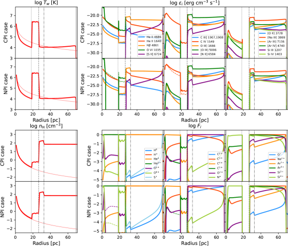
Figure 3: Top Panels: The gas temperature profiles ($T_{w}$ [K]; left panels) along with the adiabatic prediction (red dashed line), and the line emissivities ($\epsilon_{i}$ [erg cm^-3 s^-1]; right panels) of the superwind models on a logarithmic scale, from top to bottom, in the CPI (collisional ionization $+$ photoionization) cases from Danehkar et al. (2021) and NPI (non-equilibrium photoionization) cases (§ 3), for wind speed $V_{\infty}=457$ km s^-1, metallicity $\hat{Z}\equiv Z/$Z${}_{\odot}=0.5$, mass-loading rate $\dot{M}_{\rm sc}=0.607\times 10^{-2}$ M_⊙ yr^-1, cluster radius $R_{\rm sc}=1$ pc, and age $t=1$ Myr, surrounded by the ambient medium with density $n_{\rm amb}=100$ cm^-3 and temperature $T_{\rm amb}$ determined by cloudy, producing a wind model in the CB mode (described in § 2). The O vi and C iv emissivity profiles predicted by the CPI model are shown by dashed lines in the NPI panel. Bottom Panels: The hydrogen density profiles ($n_{\rm H}$ [cm^-3]; left panels) along with the adiabatic prediction (red dashed lines), and the ionic fractions ($F_{i}$; right panels) on a logarithmic scale for the CPI and NPI cases. The start and end of the hot bubble (region b), the end of the shell (region c), and the Strömgren radius are shown by dotted, dashed, dash-dotted, and solid lines (gray color), respectively. The ionic fractions predicted by the CPI model are plotted by dashed lines in the NPI panel. The plots for all the models (192 images) are available in the interactive figure in the online journal. The interactive figure includes menu options to browse all the models by varying $V_{\infty}$, $Z/$Z_⊙, $\dot{M}_{\rm sc}$, and $n_{\rm amb}$.

As described in Paper II, we generate the cloudy models for the fiducial, $Z/$Z${}_{\odot}=1$ model using ISM abundances from Savage et al. (1977) and O/H from Meyer et al. (1998), along with their depletion factors, and $Z$-parameterized C/O ratio according to the metallicity–C/O correlations from Garnett et al. (1999). The assumed baseline abundances of elements heavier than helium are also scaled down by cloudy for $Z/$Z${}_{\odot}=0.5$, $0.25$, and $0.125$. In our cloudy models, we also incorporate typical ISM dust grains with $M_{\rm d}/M_{\rm Z}=0.2$ found by De Vis et al. (2019) for typical galaxies. Our cloudy NPI models similarly use an SED generated by Starburst99 (Levesque et al., 2012; Leitherer et al., 2014) for a fixed SSC mass of $2.05\times 10^{6}$ M_⊙ at all metallicities and age of 1 Myr using Geneva population grids with stellar rotation (Ekström et al., 2012; Georgy et al., 2012, 2013), Pauldrach/Hillier atmosphere models (Hillier & Miller, 1998; Pauldrach et al., 2001), and an initial mass function (IMF) with the Salpeter slope $\alpha=2.35$ for stellar mass range 0.5–150 M_⊙. Details of our Starburst99 settings can be found in Paper II, together with the model outputs, including the predicted ionizing luminosity ($L_{\rm ion}$) required for our NPI calculations.

4 Emission Line Predictions

In this section, we describe the volume emissivities of emission lines calculated by cloudy for the NPI (non-equilibrium photoionization) models, which are used to produce luminosities. Previously, we provided the results for the PI (pure photoionization) and CPI (collisional ionization plus photoionization) models in Paper II.

For comparison with the CPI models (Paper II), Figure 3 presents the emissivities produced for different emission lines as a function of radius for both the CPI and NPI models (top-right panels). The CPI model also supplies the NPI model with the emissivity profiles of the ambient medium that were also calculated using the ambient temperature structure from the PI model as described in Paper II. The emissivities for the outflow region of the NPI model are calculated using the SED ionizing source, hydrodynamic NEI states, and hydrodynamic physical conditions ($T_{w}$ and $n_{w}$). Figure 3 also shows the ionic fractions for both the CPI and NPI models (bottom-right panels). Temperature and density profiles are also presented in Figure 3 (left panels).

In Paper II, we classified our models as optically thin if their ambient media beyond the shell are ionized (H⁺) in the associated PI models. For the ambient media in the optically thick NPI models, we use the volume emissivity profile from the CPI cloudy models up to $\sim 2$ pc after the shell inner boundary, where the temperature profile in our hydrodynamic simulations starts to be isothermal.

The luminosity $L_{\lambda}$ of each emission line at wavelength $\lambda$ is determined by taking the integrals of the volume emissivity $\epsilon_{\lambda}(r)$ as follows (see Appendix A in Paper II):

$$L_{\lambda}=\int^{2\pi}_{\varphi=0}\int^{R_{\rm aper}}_{R=0}\left[2\int^{R_{\rm max}}_{r=R}\frac{\epsilon_{\lambda}(r)}{\sqrt{r^{2}-R^{2}}}rdr\right]RdRd\varphi,$$ (7)

where $r$ is the radial distance of the volume emissivity from the center, $R$ the projected radius from the center, $R_{\rm aper}$ the boundary radius of the circular aperture used for the luminosity integration, and $R_{\rm max}$ the maximum radius of the boundary in the line of sight. We set $R_{\rm aper}=R_{\rm max}=R_{\rm Str}$ for radiation-bounded models, and $R_{\rm aper}=R_{\rm max}=R_{\rm shell}$ for density-bounded models, where $R_{\rm shell}$ is the exterior radius of the shell and $R_{\rm Str}$ is the Strömgren radius. As in Paper II, we also generate partially density-bounded models that are radiation-bounded in the line of sight, but for a density-bounded aperture: $R_{\rm aper}=R_{\rm shell}$ and $R_{\rm max}=R_{\rm Str}$.

The emission-line luminosities derived for radiation-bounded, partially density-bounded, and density-bounded NPI models are listed in Table 1. The tables for all the NPI model grids are provided in the machine-readable format in Appendix A.

4.1 UV Diagnostic Diagrams

We now generate the UV diagnostic diagrams using the emission line luminosities obtained from the emissivities predicted by our NPI models, which include various wind modes such as CC and CB. They cover the parameter space of metallicity $Z$, mass-loading $\dot{M}_{\rm sc}$, wind velocity $V_{\infty}$, and ambient density $n_{\rm amb}$. UV diagnostics diagrams have been used to identify star-forming and active galaxies (Feltre et al., 2016; Gutkin et al., 2016; Hirschmann et al., 2019).

Figures 4 and 5 show O iii] $\lambda\lambda$1661,1666/He ii $\lambda$1640 versus C iv $\lambda\lambda$1548,1551/C iii] $\lambda\lambda$1907,1909 and C iv $\lambda\lambda$1548,1551/He ii $\lambda$1640, for our radiation-bounded and partially density-bounded models, respectively. As seen in Figure 4, the O iii]/He ii and C iv/C iii] ratios decrease with an increase in the metallicity. However, the radiation-bounded models with $Z/$Z${}_{\odot}=1$ that experience strong radiative cooling produce higher values of the C iv/C iii] ratio. Moreover, we notice some slight enhancements in the C iv/C iii] ratio in the models with $Z/$Z${}_{\odot}=0.5$ and $\dot{M}_{\rm sc}$ $\geqslant$ $10^{-2}\hat{Z}^{0.72}$ M${}_{\odot}/$yr, where strong radiative cooling occurs. Cooling produces strong C iv emission within the free-expanding wind region, displacing some models relative to adiabatic ones. For the models with lower mass-loading rates ($\dot{M}_{\rm sc}$ $\leqslant$ $10^{-3}\hat{Z}^{0.72}$ M${}_{\odot}/$yr) and lower metallicity ($Z/$Z${}_{\odot}\leqslant 0.5$), radiative cooling is not strong enough to generate significant C iv emission. In the partially density-bounded models having radiatively cooled winds (Figure 5), enhanced C iv emission is more pronounced, since these models are more strongly weighted toward emission produced in the free wind and the shell. On the other hand, O iii] and C iii] are less sensitive to strong radiative cooling, so they do not demonstrate any significant departures from the adiabatic wind models.

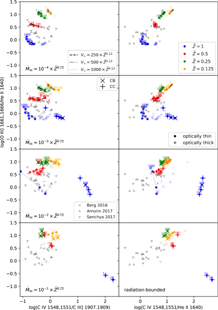
Figure 4: The UV diagnostic diagrams plotted O iii] $\lambda\lambda$1661,1666/He ii $\lambda$1640 versus C iv $\lambda\lambda$1548,1551/C iii] $\lambda\lambda$1907,1909 (left) and O iii] $\lambda\lambda$1661,1666/He ii $\lambda$1640 versus C iv $\lambda\lambda$1548,1551/He ii $\lambda$1640 (right panels) for the fully radiation-bounded NPI models with mass-loading rates $\log\dot{M}_{\rm sc}=-4$, $-3$, $-2$, and $-1$ M${}_{\odot}/$yr (from top to bottom), ambient densities $n_{\rm amb}=1$, 10, $10^{2}$, and $10^{3}$ cm^-3 (labeled on plots), metallicities $\hat{Z}\equiv Z/$Z${}_{\odot}=1$ (blue), $0.5$ (red), $0.25$ (green), and $0.125$ (yellow color), and wind velocities $V_{\infty}=250$ (dashed), $500$ (dash-dotted), and $1000$ km s^-1 (dotted lines). For the sub-solar models, we use the solar model parameters scaled as $\dot{M}_{\rm sc}\varpropto Z^{0.72}$ and $V_{\infty}\varpropto Z^{0.13}$. The optically thin and thick models are plotted by filled and empty circles, respectively. The wind catastrophic cooling (CC) and catastrophic cooling with the bubble (CB) modes are labeled by the plus (’$+$’) and cross (’$\times$’) symbols, respectively. The CPI results from Paper II are shown by lightly shaded colors. The plotted observations are from Berg et al. (2016), Amorín et al. (2017), and Senchyna et al. (2017).

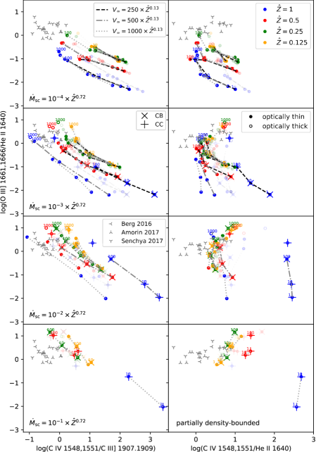
Figure 5: The same as Figure 4, but for the partially density-bounded models.

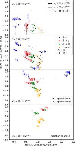
Figure 6: The UV diagnostic diagrams plotted O vi $\lambda\lambda$1032,1038/He ii $\lambda$1640 versus C iv $\lambda\lambda$1548,1551/He ii $\lambda$1640 for the radiation-bounded NPI models. Symbols and line types are as in Figure 4. The CPI results are shown by lightly shaded colors.

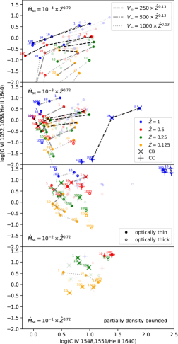
Figure 7: The same as Figure 6, but for the partially density-bounded models.

Similarly, we present diagnostic diagrams for O vi $\lambda\lambda$1032,1038/He ii $\lambda$1640 versus C iv $\lambda\lambda$1549,1551/He ii $\lambda$1640 in Figures 6 and 7 for radiation-bounded, and partially density-bounded, respectively, which may be compared to those in Paper II (CPI results plotted by lightly shaded colors). The highly ionized O vi $\lambda\lambda$1032,1038 emission has been suggested as a diagnostic tool for catastrophic cooling winds (Gray et al., 2019b). At first glance, it seems that the C iv $\lambda\lambda$1548,1551 emission rather O vi $\lambda\lambda$1032,1038 is significantly enhanced in the models with catastrophic cooling. However, we also see in Figure 6 that strong radiative cooling considerably increases the O vi emission in the models with $\dot{M}_{\rm sc}$ $=$ $10^{-2}$ and $10^{-3}\times\hat{Z}^{0.72}$ M${}_{\odot}/$yr at $Z/$Z${}_{\odot}=0.5$ and $0.25$, while the C iv emission from the radiatively cooled winds is slightly increased in the models with $\dot{M}_{\rm sc}$ $=$ $10^{-2}\hat{Z}^{0.72}$ M${}_{\odot}/$yr, remaining similar to that from the adiabatic models for $\dot{M}_{\rm sc}$ $=$ $10^{-3}\hat{Z}^{0.72}$ M${}_{\odot}/$yr. While the C iv/He ii emission-line ratio expected from the NPI models may be employed to distinguish between radiatively cooling and adiabatic winds in metal-rich ($Z/$Z${}_{\odot}\gtrsim 0.5$) regions, the non-equilibrium photoionized O vi/He ii emission-line ratio could be used as a diagnostic of radiative cooling in metal-poor ($Z/$Z${}_{\odot}\lesssim 0.5$) H ii regions typical of starburst galaxies.

Previously, we also saw enhancement of radiation-bounded O vi emission predicted by the CPI models for radiatively cooled outflows with mass-loading rates $\geqslant 10^{-2}$ M${}_{\odot}/$yr in metal-poor regions $Z/$Z${}_{\odot}\leqslant 0.5$ (Figure 11 in Paper II). The enhanced O vi/He ii emission-line ratios produced by non-equilibrium photoionization processes in metal-poor H ii regions is similar to that seen in combined collisional ionization and photoionization processes, whereas the substantially enhanced C iv/He ii ratios in the NPI models are not seen in the CPI models presented in Paper II. As seen in Figure 3, the O vi emission is mostly generated in the central part of the free wind close to the SSC and in the hot bubble region in our NPI models. The O vi emissivity profile for NPI is different from that for the CPI model (see Figure 3), while the enhanced C iv emissivity profile in NPI looks roughly similar to the CPI model, except for some sharp peaks in O vi and C iv in the CPI model in the interface region between the bubble (CIE) and the shell (PIE).

It can be seen in Figures 6 and 7 that the O vi emission from the adiabatic winds rises with increasing metallicity and mass deposition. This trend in the adiabatic winds of the NPI models that is similar to those of the CPI models in Paper II is more noticeable in the partially density-bounded models in Figure 7. The enhanced O vi emission at $Z/$Z${}_{\odot}<1$ agrees with Paper I suggesting that O vi could be enhanced in radiatively cooled winds, although not significantly for $Z/$Z${}_{\odot}=1$. However, the C iv emission appears to be a useful diagnostic of radiative cooling at $Z/$Z${}_{\odot}=1$. Thus, to identify strong radiative cooling, it is necessary to know the metallicity. Moreover, information on the ambient density and mass loading further help to diagnose radiatively cooling superwinds.

Figures 4–7 also include optically thick NPI models. In particular, the enhanced O vi and C iv emission are also seen in some of the optically thick NPI models with strong radiative cooling. While C iv emission did not increase much in the CPI model in Paper II, substantially enhanced C iv emission is seen in the radiatively cooling wind models with $Z/$Z${}_{\odot}=1$, as well as those with $Z/$Z${}_{\odot}=0.5$ and $\dot{M}_{\rm sc}\geqslant 10^{-2}$ M${}_{\odot}/$yr.

We note that our models do not account for radiative transfer, in particular, absorption and reemission by dust and other species. We incorporate metal depletion into our hydrodynamic simulations and include dust grains and depletion in our cloudy calculations using the NEI states and physical conditions produced by maihem. Including dust grains as separate species with distinctive equations of state in maihem hydrodynamic simulations would contribute to significant changes in the UV diagnostic diagrams, since dust grains can affect thermal structures and absorb radiation fields. Moreover, NEI cooling rates can also be affected by dust grains (Richings et al., 2014). Currently, we assume typical ISM dust grains with $M_{\rm d}/M_{\rm Z}=0.2$, in typical galaxies (De Vis et al., 2019).

5 Applications for Observations

Our NPI models predict that radiatively cooling outflows could contribute to the higher excitation seen in extreme starbursts and GPs. In Figures 4–5, we plot UV observations of nearby and distant starburst galaxies (Richard et al., 2011; Masters et al., 2014; Berg et al., 2016; Amorín et al., 2017; Senchyna et al., 2017). Their physical properties are roughly similar to those considered for our models. The nearby dwarf galaxies analyzed by Berg et al. (2016) and Senchyna et al. (2017) have oxygen abundances of $12+\log($O/H$)\approx 7.6$ and $\lesssim 8.3$, respectively; and the more distant star-forming galaxies studied by Amorín et al. (2017) have a mean oxygen abundance of $12+\log($O/H$)\approx 7.6$.

In particular, our models show that O vi $\lambda\lambda$1032,1038 emission is produced in radiatively cooling outflows, as suggested by Heckman et al. (2001), Otte et al. (2003), Hayes et al. (2016), and Li et al. (2017). As seen in Figures 6–7, particularly in the metal-poor ($Z/$Z${}_{\odot}\leqslant 0.5$) models, the O vi $\lambda\lambda$1032,1038 emission lines predicted by the radiative cooling wind models are higher than those expected by the adiabatic wind models with the same metallicity and mass loading.

Strong O vi emission indeed is sometimes seen in young starbursts. For example, Marques-Chaves et al. (2021) find clear P-Cygni emission in O vi, Si iv, and C iv, in a luminous LyC emitter at $z=3.2$. The strength of these features is hard to explain with a simple starburst stellar population. While the broad line profiles must be dominated by stars, it may be possible that a component from radiatively cooling outflows could contribute. Similarly, O vi $\lambda\lambda$1032,1038 emission lines with P Cygni profiles were also identified in Haro 11 (Bergvall et al., 2006; Grimes et al., 2007) and other starbursting blue compact galaxies (Izotov et al., 2018). O vi emission was detected by Otte et al. (2003) toward a soft X-ray bubble in the star-forming galaxy NGC 4631 that could be associated with cooling, galactic outflows ($v_{\rm w}\sim 50$–100 km s^-1). More recently, O vi imaging of the starburst SDSS J1156$+$5008 by Hayes et al. (2016) shows an extended halo, and its spectrum also contains O vi absorption outflowing with an average velocity of $380$ km s^-1. Observations of the dwarf starburst galaxy NGC 1705 studied by Heckman et al. (2001) revealed a low-speed outflow ($v_{\rm w}=77$ km s^-1) in O vi absorption, surrounded by a $\sim 10^{4}$ K medium arising in a conductive interface between the hot superbubble and cool outer shell, and which cannot be explained by a simple adiabatic superbubble model. The physical properties of these starburst galaxies are in the parameter ranges used by our models.

Our models with catastrophically cooling winds at $Z/$Z${}_{\odot}\geqslant 0.5$ also demonstrate prominent C iv emission lines relative to adiabatic wind models. Interestingly, Senchyna et al. (2017) found strong C iv emission in metal-poor star-forming regions associated with minimal stellar wind features and $12+\log($O/H$)\lesssim 8.3$ ($Z/$Z${}_{\odot}\lesssim 0.6$). Similarly, Berg et al. (2019a) detected intense C iv $\lambda\lambda$1548,1551 emission lines from two extreme UV emission-line galaxies demonstrating little-to-no outflows (Berg et al., 2019a) at $12+\log($O/H$)\approx 7.5$ ($Z/$Z${}_{\odot}\sim 0.1$), as well as other nearby metal-poor high-ionization dwarf galaxies (Berg et al., 2019b). Our non-equilibrium photoionization models predict that such intense C iv emission could be prevalent in radiatively cooling winds with $Z/$Z${}_{\odot}\gtrsim 0.5$, but if these objects have C-enhanced abundances, radiatively cooling C iv could contribute to the unusually strong emission at lower metallicities. With constraints on metallicity and mass loading, it is becomes possible to distinguish between adiabatic and radiatively cooling outflows.

6 Summary and Conclusions

We have presented here our grid of non-equilibrium photoionization (NPI) models constructed using non-equilibrium ionization (NEI) states and physical conditions predicted by our hydrodynamic simulations previously presented in Paper II. We use the same ionizing SED associated with a total stellar mass of $2.05\times 10^{6}$ M_⊙, and the same parameter space of the metallicity ($\hat{Z}\equiv Z/$Z${}_{\odot}=1$, $0.5$, $0.25$, $0.125$), mass-loading rate ($\dot{M}_{\rm sc}$ $=$ $10^{-1},\ldots,10^{-4}\times\hat{Z}^{0.72}$ M${}_{\odot}\,$yr^-1), wind velocity ($V_{\infty}$ $=$ $250,500,1000\times\hat{Z}^{0.13}$ km s^-1), and ambient density ($n_{\rm amb}$ $=$ $1,\ldots,10^{3}$ cm^-3) employed in Paper II. The non-equilibrium photoionization modeling is carried out using the same non-CIE approach implemented by Gray et al. (2019a).

Previously, we identified the parameter space (in $\hat{Z}$, $\dot{M}_{\rm sc}$, $V_{\infty}$, $n_{\rm amb}$) associated with strongly radiative cooling, and classified them under different wind modes based on departures from the adiabatic solutions and presence/absence of the hot bubble within 1 Myr (see § 4 in Danehkar et al., 2021). We found that low heating efficiency and high mass deposition are linked to strong radiative cooling effects, while the presence of a hot bubble is not a reliable indicator of either adiabatic or radiatively cool outflows. We also employed physical conditions to predict emission lines for combined collisional ionization and photoionization (CPI) processes without considering non-equilibrium ionization conditions.

In this paper, we utilize NEI states and physical proprieties generated by time-dependent non-equilibrium processes to calculate volume emissivities of UV and optical emission lines with cloudy, and their luminosities for radiation-bounded and partially density-bounded models. We use the predicted line luminosities of UV lines studied in Paper II to compile diagnostic diagrams for comparison with observations of star-forming regions.

The radiation-bounded UV emission-line ratios predicted by our NPI models are generally located in our diagnostic diagrams where both nearby and distant starburst galaxies with the modeled physical properties are observed (see Figures 4–5), similar to what is seen for the CPI models in Paper II. However, we see some noticeable differences between the emission-line ratios made by our NPI models and those by the CPI models that are due to NEI conditions. Our NPI models demonstrate that radiative cooling strongly enhances C iv emission in metal-rich ($Z/$Z${}_{\odot}\geqslant 0.5$) regions and also increases O vi emission in metal-poor ($Z/$Z${}_{\odot}\leqslant 0.5$) regions that are typical of starbursts. However, some constraints on the metallicity and mass loading are necessary in order to diagnose superwinds with strongly radiative cooling.

The enhanced C iv $\lambda\lambda$1548,1551 and O vi $\lambda\lambda$1032,1038 in catastrophically cooling outflows were previously suggested based on non-equilibrium ionization models by Gray et al. (2019a) and Gray et al. (2019b). Moreover, hydrodynamic simulations of starburst-driven galactic outflows by Cottle et al. (2018) could not adequately produce the observed O vi, implying possible implications of nonequilibrium ionization processes. Previously, time-dependent calculations of the NEI states by de Avillez & Breitschwerdt (2012) showed the production of O vi in the thermally stable ($\sim 10^{\textrm{3.9--4.2}}$) and unstable ($\sim 10^{\textrm{4.2--5}}$) regimes having temperatures below that required for O vi in collisional ionization. Our photoionization calculations done with NEI states demonstrate the feasibility of intense O vi made by radiative cooling in metal-poor environments.

The occurrence of catastrophic cooling and the formation of C iv and O vi emission should also be investigated under different physical conditions such as compact and ultra-compact H ii regions where cluster dimensions are much smaller than our typical SSC radius (1 pc) and stellar masses are lower than our SSC mass. It is also necessary to explore different dust proprieties that are typically seen in distant star-forming galaxies. Future studies on the wide range of physical parameters will help us broaden our understanding of radiatively cooling outflows and their associated emission lines.

Appendix A Supplementary Material

The interactive figure (192 images) of Figure 3 is available in the electronic edition of this article, and is archived on Zenodo (doi:10.5281/zenodo.6601127). This interactive figure is also hosted at: https://galacticwinds.github.io/superwinds.

The 3 machine-readable tables with the emission-line data (including Table 1) is available in the electronic edition of this article. Each file is named as table_case_bound.dat, such as table_NPI_radi.dat, where case is for the ionization case (NPI: non-equilibrium photoionization), and bound for the optical depth model (radi: fully radiation-bounded, pden: partially density-bounded, and dens: fully density-bounded). Each file contains the following information:

Table 1: Emission line luminosities calculated by the NPI models on a logarithmic scale (unit in erg/s) with different optical depth configurations (see Appendix A for more information).

Emission Line	radiation-bound	part.density-bound	density-bound
Ly$\alpha$ $\lambda$1216	40.561	40.151	40.025
H$\alpha$ $\lambda$6563	40.791	40.463	40.186
H$\beta$ $\lambda$4861	40.352	40.024	39.748
He i $\lambda$5876	39.443	39.118	38.843
He i $\lambda$6678	38.876	38.550	38.275
He i $\lambda$7065	39.121	38.818	38.532
He ii $\lambda$1640	38.767	38.685	38.588
He ii $\lambda$4686	36.311	36.238	36.153
C ii $\lambda$1335	38.402	37.941	37.546
C ii $\lambda$2326	38.177	37.360	35.930
C iii $\lambda$977	38.574	38.347	38.117
C iii] $\lambda$1909	39.878	39.261	38.669
C iii $\lambda$1549	36.902	36.679	36.451
C iv $\lambda$1549	39.529	39.290	39.177
[N i] $\lambda$5200	36.092	35.172	31.005
[N ii] $\lambda$5755	37.051	36.207	34.730
[N ii] $\lambda$6548	38.179	37.337	35.992
[N ii] $\lambda$6583	38.649	37.806	36.462
N iii $\lambda$1750	39.343	38.679	37.966
N iii $\lambda$991	39.062	38.820	38.584
N iv $\lambda$1486	39.173	38.774	38.453
N v $\lambda$1240	39.593	39.593	39.593
O i $\lambda$1304	38.011	37.092	33.792
[O i] $\lambda$6300	36.234	35.323	31.558
[O i] $\lambda$6364	35.739	34.827	31.063
[O ii] $\lambda$3726	38.609	37.842	36.955
[O ii] $\lambda$3729	38.753	37.981	37.055
[O ii] $\lambda$7323	37.364	36.815	36.385
[O ii] $\lambda$7332	37.281	36.729	36.296
O iii] $\lambda$1661	38.791	38.244	37.778
O iii] $\lambda$1666	39.262	38.715	38.250
[O iii] $\lambda$2321	38.549	38.066	37.670
[O iii] $\lambda$4363	39.148	38.665	38.270
[O iii] $\lambda$4959	40.568	40.165	39.835
[O iii] $\lambda$5007	41.043	40.640	40.310
…

• Table 1 is published in its entirety in the machine-readable format. A portion is shown here for guidance regarding its form and content.

• Model parameters for this example are as follows: metallicity $Z/$Z${}_{\odot}=0.5$, mass-loading rate $\dot{M}_{\rm sc}=0.607\times 10^{-2}$ M_⊙ yr^-1, actual wind velocity $V_{\infty}=457$ km s^-1, SSC radius $R_{\rm sc}=1$ pc, stellar mass $M_{\star}=2.05\times 10^{6}$ M_⊙, age $t=1$ Myr, ambient density $n_{\rm amb}=100$ cm^-3, and ambient temperature $T_{\rm amb}$ estimated by cloudy.

• metal: metallicity $\hat{Z}\equiv Z/$Z${}_{\odot}=1$, $0.5$, $0.25$, $0.125$.

• dMdt: mass-loading rate $\dot{M}_{\rm sc}=10^{-1}$, $10^{-2}$, $10^{-3}$, $10^{-4}\times\hat{Z}^{0.72}$ M_⊙ yr^-1.

• Vinf: wind terminal velocity $V_{\infty}=250$, $500$, $1000\times\hat{Z}^{0.13}$ km s^-1.

• Rsc: SSC radius $R_{\rm sc}=1$ pc.

• age: current age $t=1$ Myr.

• Mstar: total stellar mass $M_{\star}=2.05\times 10^{6}$ M_⊙.

• logLion: ionizing luminosity $\log L_{\rm ion}$ (erg/s).

• Namb: ambient density $n_{\rm amb}=1$, 10, $10^{2}$, $10^{3}$ cm^-3.

• Tamb: mean ambient temperature $T_{\rm amb}$ from cloudy.

• Rmax: maximum radius $R_{\rm max}$ (pc) for the surface brightness integration.

• Raper: aperture radius $R_{\rm aper}$ (pc) for the luminosity integration.

• Rshell: shell exterior radius $R_{\rm shell}$ (pc).

• Rstr: Strömgren radius $R_{\rm str}$ (pc) from cloudy.

• Rbin: bubble interior radius $R_{\rm b,in}$ (pc).

• Rbout: bubble exterior radius $R_{\rm b,out}$ (pc) or shell interior radius.

• Tbubble: median temperature $T_{\rm bubble}$ of the bubble.

• Tadi: median adiabatic temperature $T_{\rm adi,med}$ of the expanding wind.

• Twind: median radiative temperature $T_{\rm w,med}$ of the expanding wind.

• logUsp: logarithmic ionization parameter $\log U_{\rm sph}$ in a spherical geometry from cloudy.

• thin: optically thin (1) or thick (0) model.

• mode: the cooling/heating radiative/adiabatic modes: 1 (AW: adiabatic wind), 2 (AB: adiabatic bubble), 3 (AP: adiabatic, pressure-confined), 4 (CC: catastrophic cooling), 5 (CB: catastrophic cooling bubble), and 6 (CP: catastrophic cooling, pressure-confined), described in details by Danehkar et al. (2021).

• H_1_1216, H_1_6563, …, Ar_5_7006: luminosities of the emission lines Ly$\alpha$ $\lambda$1216 Å, H$\alpha$ $\lambda$6563 Å, …, [Ar v] $\lambda$7006 Å, respectively.

ORCID iDs

A. Danehkar https://orcid.org/0000-0003-4552-5997

M. S. Oey https://orcid.org/0000-0002-5808-1320

W. J. Gray https://orcid.org/0000-0001-9014-3125

References

- Amorín et al. (2017) Amorín, R., Fontana, A., Pérez-Montero, E., et al. 2017, Nature Astron., 1, 0052
- Badnell (2006) Badnell, N. R. 2006, ApJS, 167, 334
- Berg et al. (2019a) Berg, D. A., Chisholm, J., Erb, D. K., et al. 2019a, ApJ, 878, L3
- Berg et al. (2019b) Berg, D. A., Erb, D. K., Henry, R. B. C., Skillman, E. D., & McQuinn, K. B. W. 2019b, ApJ, 874, 93
- Berg et al. (2016) Berg, D. A., Skillman, E. D., Henry, R. B. C., Erb, D. K., & Carigi, L. 2016, ApJ, 827, 126
- Bergvall et al. (2006) Bergvall, N., Zackrisson, E., Andersson, B. G., et al. 2006, A&A, 448, 513
- Bolatto et al. (2013) Bolatto, A. D., Warren, S. R., Leroy, A. K., et al. 2013, Nature, 499, 450
- Bryans et al. (2006) Bryans, P., Badnell, N. R., Gorczyca, T. W., et al. 2006, ApJS, 167, 343
- Cantó et al. (2000) Cantó, J., Raga, A. C., & Rodríguez, L. F. 2000, ApJ, 536, 896
- Castor et al. (1975) Castor, J., McCray, R., & Weaver, R. 1975, ApJ, 200, L107
- Chevalier & Clegg (1985) Chevalier, R. A. & Clegg, A. W. 1985, Nature, 317, 44
- Cottle et al. (2018) Cottle, J. N., Scannapieco, E., & Brüggen, M. 2018, ApJ, 864, 96
- Cox & Tucker (1969) Cox, D. P. & Tucker, W. H. 1969, ApJ, 157, 1157
- Danehkar et al. (2021) Danehkar, A., Oey, M. S., & Gray, W. J. 2021, ApJ, 921, 91, (Paper II)
- de Avillez & Breitschwerdt (2012) de Avillez, M. A. & Breitschwerdt, D. 2012, ApJ, 761, L19
- De Vis et al. (2019) De Vis, P., Jones, A., Viaene, S., et al. 2019, A&A, 623, A5
- della Ceca et al. (1996) della Ceca, R., Griffiths, R. E., Heckman, T. M., & MacKenty, J. W. 1996, ApJ, 469, 662
- Dopita & Sutherland (2003) Dopita, M. A. & Sutherland, R. S. 2003, Astrophysics of the Diffuse Universe (Berlin, New York: Springer)
- Ekström et al. (2012) Ekström, S., Georgy, C., Eggenberger, P., et al. 2012, A&A, 537, A146
- Fabian et al. (1984) Fabian, A. C., Nulsen, P. E. J., & Canizares, C. R. 1984, Nature, 310, 733
- Feltre et al. (2016) Feltre, A., Charlot, S., & Gutkin, J. 2016, MNRAS, 456, 3354
- Ferland et al. (2017) Ferland, G. J., Chatzikos, M., Guzmán, F., et al. 2017, RMxAA, 53, 385
- Ferland et al. (1998) Ferland, G. J., Korista, K. T., Verner, D. A., et al. 1998, PASP, 110, 761
- Ferland et al. (2013) Ferland, G. J., Porter, R. L., van Hoof, P. A. M., et al. 2013, RMxAA, 49, 137
- Fryxell et al. (2000) Fryxell, B., Olson, K., Ricker, P., et al. 2000, ApJS, 131, 273
- Garnett et al. (1999) Garnett, D. R., Shields, G. A., Peimbert, M., et al. 1999, ApJ, 513, 168
- Georgy et al. (2013) Georgy, C., Ekström, S., Eggenberger, P., et al. 2013, A&A, 558, A103
- Georgy et al. (2012) Georgy, C., Ekström, S., Meynet, G., et al. 2012, A&A, 542, A29
- Gnat & Ferland (2012) Gnat, O. & Ferland, G. J. 2012, ApJS, 199, 20
- Gnat & Sternberg (2007) Gnat, O. & Sternberg, A. 2007, ApJS, 168, 213
- Gray et al. (2019a) Gray, W. J., Oey, M. S., Silich, S., & Scannapieco, E. 2019a, ApJ, 887, 161, (Paper I)
- Gray & Scannapieco (2016) Gray, W. J. & Scannapieco, E. 2016, ApJ, 818, 198
- Gray et al. (2015) Gray, W. J., Scannapieco, E., & Kasen, D. 2015, ApJ, 801, 107
- Gray et al. (2019b) Gray, W. J., Scannapieco, E., & Lehnert, M. D. 2019b, ApJ, 875, 110
- Grimes et al. (2007) Grimes, J. P., Heckman, T., Strickland, D., et al. 2007, ApJ, 668, 891
- Gutkin et al. (2016) Gutkin, J., Charlot, S., & Bruzual, G. 2016, MNRAS, 462, 1757
- Harris et al. (2020) Harris, C. R., Millman, K. J., van der Walt, S. J., et al. 2020, Nature, 585, 357
- Hayes et al. (2016) Hayes, M., Melinder, J., Östlin, G., et al. 2016, ApJ, 828, 49
- Heckman et al. (1990) Heckman, T. M., Armus, L., & Miley, G. K. 1990, ApJS, 74, 833
- Heckman et al. (2001) Heckman, T. M., Sembach, K. R., Meurer, G. R., et al. 2001, ApJ, 554, 1021
- Hillier & Miller (1998) Hillier, D. J. & Miller, D. L. 1998, ApJ, 496, 407
- Hirschmann et al. (2019) Hirschmann, M., Charlot, S., Feltre, A., et al. 2019, MNRAS, 487, 333
- Hunter (2007) Hunter, J. D. 2007, Comput. Sci. Eng., 9, 90
- Izotov & Thuan (1999) Izotov, Y. I. & Thuan, T. X. 1999, ApJ, 511, 639
- Izotov et al. (2018) Izotov, Y. I., Worseck, G., Schaerer, D., et al. 2018, MNRAS, 478, 4851
- James et al. (2009) James, B. L., Tsamis, Y. G., Barlow, M. J., et al. 2009, MNRAS, 398, 2
- James et al. (2013) James, B. L., Tsamis, Y. G., Walsh, J. R., Barlow, M. J., & Westmoquette, M. S. 2013, MNRAS, 430, 2097
- Jaskot et al. (2017) Jaskot, A. E., Oey, M. S., Scarlata, C., & Dowd, T. 2017, ApJ, 851, L9
- Kafatos (1973) Kafatos, M. 1973, ApJ, 182, 433
- Krause et al. (2016) Krause, M. G. H., Charbonnel, C., Bastian, N., & Diehl, R. 2016, A&A, 587, A53
- Lee (2013) Lee, D. 2013, J. Comput. Phys., 243, 269
- Lee & Deane (2009) Lee, D. & Deane, A. E. 2009, J. Comput. Phys., 228, 952
- Lee et al. (2009) Lee, D., Deane, A. E., & Federrath, C. 2009, ASP Conf. Ser., Vol. 406, A New Multidimensional Unsplit MHD Solver in FLASH3, ed. N. V. Pogorelov, E. Audit, P. Colella, & G. P. Zank, 243
- Leitherer et al. (2014) Leitherer, C., Ekström, S., Meynet, G., et al. 2014, ApJS, 212, 14
- Leitherer et al. (1999) Leitherer, C., Schaerer, D., Goldader, J. D., et al. 1999, ApJS, 123, 3
- Leroy et al. (2015) Leroy, A. K., Walter, F., Martini, P., et al. 2015, ApJ, 814, 83
- Levesque et al. (2012) Levesque, E. M., Leitherer, C., Ekstrom, S., Meynet, G., & Schaerer, D. 2012, ApJ, 751, 67
- Li et al. (2017) Li, M., Bryan, G. L., & Ostriker, J. P. 2017, ApJ, 835, L10
- Lochhaas et al. (2020) Lochhaas, C., Bryan, G. L., Li, Y., Li, M., & Fielding, D. 2020, MNRAS, 493, 1461
- Lochhaas et al. (2018) Lochhaas, C., Thompson, T. A., Quataert, E., & Weinberg, D. H. 2018, MNRAS, 481, 1873
- Marques-Chaves et al. (2021) Marques-Chaves, R., Schaerer, D., Álvarez-Márquez, J., et al. 2021, MNRAS, 507, 524
- Martin (1999) Martin, C. L. 1999, ApJ, 513, 156
- Masters et al. (2014) Masters, D., McCarthy, P., Siana, B., et al. 2014, ApJ, 785, 153
- Meyer et al. (1998) Meyer, D. M., Jura, M., & Cardelli, J. A. 1998, ApJ, 493, 222
- Mokiem et al. (2007) Mokiem, M. R., de Koter, A., Vink, J. S., et al. 2007, A&A, 473, 603
- Oey et al. (2017) Oey, M. S., Herrera, C. N., Silich, S., et al. 2017, ApJ, 849, L1
- Oppenheimer & Schaye (2013) Oppenheimer, B. D. & Schaye, J. 2013, MNRAS, 434, 1043
- Ott et al. (2005a) Ott, J., Walter, F., & Brinks, E. 2005a, MNRAS, 358, 1453
- Ott et al. (2005b) Ott, J., Weiss, A., Henkel, C., & Walter, F. 2005b, ApJ, 629, 767
- Otte et al. (2003) Otte, B., Murphy, E. M., Howk, J. C., et al. 2003, ApJ, 591, 821
- Pauldrach et al. (2001) Pauldrach, A. W. A., Hoffmann, T. L., & Lennon, M. 2001, A&A, 375, 161
- Raymond et al. (1976) Raymond, J. C., Cox, D. P., & Smith, B. W. 1976, ApJ, 204, 290
- Richard et al. (2011) Richard, J., Jones, T., Ellis, R., et al. 2011, MNRAS, 413, 643
- Richings et al. (2014) Richings, A. J., Schaye, J., & Oppenheimer, B. D. 2014, MNRAS, 440, 3349
- Sarazin (1988) Sarazin, C. L. 1988, X-ray emission from clusters of galaxies (Cambridge: Cambridge University Press)
- Savage et al. (1977) Savage, B. D., Bohlin, R. C., Drake, J. F., & Budich, W. 1977, ApJ, 216, 291
- Schmutzler & Tscharnuter (1993) Schmutzler, T. & Tscharnuter, W. M. 1993, A&A, 273, 318
- Schneider et al. (2018) Schneider, E. E., Robertson, B. E., & Thompson, T. A. 2018, ApJ, 862, 56
- Senchyna et al. (2017) Senchyna, P., Stark, D. P., Vidal-García, A., et al. 2017, MNRAS, 472, 2608
- Shapiro & Moore (1976) Shapiro, P. R. & Moore, R. T. 1976, ApJ, 207, 460
- Shull & van Steenberg (1982) Shull, J. M. & van Steenberg, M. 1982, ApJS, 48, 95
- Silich & Tenorio-Tagle (2017) Silich, S. & Tenorio-Tagle, G. 2017, MNRAS, 465, 1375
- Silich et al. (2003) Silich, S., Tenorio-Tagle, G., & Muñoz-Tuñón, C. 2003, ApJ, 590, 791
- Silich et al. (2004) Silich, S., Tenorio-Tagle, G., & Rodríguez-González, A. 2004, ApJ, 610, 226
- Smith et al. (2006) Smith, L. J., Westmoquette, M. S., Gallagher, J. S., et al. 2006, MNRAS, 370, 513
- Strickland et al. (1997) Strickland, D. K., Ponman, T. J., & Stevens, I. R. 1997, A&A, 320, 378
- Sutherland & Dopita (1993) Sutherland, R. S. & Dopita, M. A. 1993, ApJS, 88, 253
- Tenorio-Tagle et al. (2005) Tenorio-Tagle, G., Silich, S., Rodríguez-González, A., & Muñoz-Tuñón, C. 2005, ApJ, 620, 217
- Tenorio-Tagle et al. (2007) Tenorio-Tagle, G., Wünsch, R., Silich, S., & Palouš, J. 2007, ApJ, 658, 1196
- Toro et al. (1994) Toro, E. F., Spruce, M., & Speares, W. 1994, Shock Waves, 4, 25
- Truelove et al. (1997) Truelove, J. K., Klein, R. I., McKee, C. F., et al. 1997, ApJ, 489, L179
- Turk et al. (2011) Turk, M. J., Smith, B. D., Oishi, J. S., et al. 2011, ApJS, 192, 9
- Turner et al. (2017) Turner, J. L., Consiglio, S. M., Beck, S. C., et al. 2017, ApJ, 846, 73
- van Leer (1979) van Leer, B. 1979, J. Comput. Phys., 32, 101
- Vasiliev (2011) Vasiliev, E. O. 2011, MNRAS, 414, 3145
- Veilleux et al. (2020) Veilleux, S., Maiolino, R., Bolatto, A. D., & Aalto, S. 2020, A&A Rev., 28, 2
- Verner et al. (1996) Verner, D. A., Ferland, G. J., Korista, K. T., & Yakovlev, D. G. 1996, ApJ, 465, 487
- Verner & Yakovlev (1995) Verner, D. A. & Yakovlev, D. G. 1995, A&AS, 109, 125
- Vink et al. (2001) Vink, J. S., de Koter, A., & Lamers, H. J. G. L. M. 2001, A&A, 369, 574
- Virtanen et al. (2020) Virtanen, P., Gommers, R., Oliphant, T. E., et al. 2020, Nature Methods, 17, 261
- Voronov (1997) Voronov, G. S. 1997, Atom. Data Nucl. Data Tabl., 65, 1
- Walsh & Roy (1989) Walsh, J. R. & Roy, J.-R. 1989, MNRAS, 239, 297
- Weaver et al. (1977) Weaver, R., McCray, R., Castor, J., Shapiro, P., & Moore, R. 1977, ApJ, 218, 377
- Weiß et al. (2005) Weiß, A., Walter, F., & Scoville, N. Z. 2005, A&A, 438, 533
- Westmoquette et al. (2014) Westmoquette, M. S., Bastian, N., Smith, L. J., et al. 2014, ApJ, 789, 94
- Wünsch et al. (2011) Wünsch, R., Silich, S., Palouš, J., Tenorio-Tagle, G., & Muñoz-Tuñón, C. 2011, ApJ, 740, 75
- Wünsch et al. (2021) Wünsch, R., Walch, S., Dinnbier, F., et al. 2021, MNRAS, 505, 3730
- Wünsch et al. (2018) Wünsch, R., Walch, S., Dinnbier, F., & Whitworth, A. 2018, MNRAS, 475, 3393