Performance Analysis for Reconfigurable Intelligent Surface Assisted MIMO Systems

Abstract

This paper investigates the maximal achievable rate for a given average error probability and blocklength for the reconfigurable intelligent surface (RIS) assisted multiple-input and multiple-output (MIMO) system. The result consists of a finite blocklength channel coding achievability bound and a converse bound based on the Berry-Esseen theorem, the Mellin transform and the mutual information. Numerical evaluation shows fast speed of convergence to the maximal achievable rate as the blocklength increases and also proves that the channel variance is a sound measurement of the backoff from the maximal achievable rate due to finite blocklength.

I Introduction

Recently, there has been a prodigious increase in the demand for higher data rates in wireless communication networks due to the escalating number of mobile and IoT devices together with dramatically increased services [1, 2, 3]. To this end, many candidate solutions have been proposed to deal with this demand, such as multiple-input multiple-output (MIMO) and millimeter-wave (mmWave)/TeraHertz (THz) communications [4, 5, 6, 7, 8]. These technologies offer significant data rate gains but have power and hardware cost limitations. Generally speaking, they can be regarded as a way to achieve higher data rates by altering transmitter and receiver features without influencing the propagation channel.

A possible approach to overcome the issues mentioned above lies in the use of the recently-developed reconfigurable intelligent surface (RIS), which consists of a massive array of scattering elements [9, 10, 11]. Since the RIS is a passive device with low energy consumption and without self-interference, it is regarded as a better technology than the backscatter and Multi-input multi-output (MIMO) relay [12, 13, 14, 15, 16, 17, 18]. The array of elements can be configured by controllers to reflect radio waves towards arbitrary angles so that we can apply phase shifts and modify polarization[19]. Unlike existing relay technologies [20, 21, 22, 23, 24], RIS can turn the hostile propagation environment into a favorable one due to its unique properties ameliorate the signal quality at the receiver side without consuming additional power.

Most prior works have demonstrated the advantages of the RIS in terms of the bit-error-rate performance and cell coverage. In contrast, this paper takes a more fundamental information-theoretic perspective on the performance of RIS-assisted MIMO communication systems at the finite blocklength regime.

Related Work: In [25], a broad mathematical framework of the RIS-assisted wireless communication system over Rayleigh fading channel was presented and then a theoretical upper bound was derived. Moreover, the authors presented the relationship between the received signal-to-noise ratio (SNR) and the number of reflecting elements, indicating that the received SNR grew considerably as the number of reflecting elements increased. Thus the reliable transmission over a noisy channel could be still accomplished at low SNRs with the support of the RIS elements. The authors of [26] investigated the coverage expansion achieved by the RIS-assisted wireless communication system over quasi-static flat Rayleigh fading channels. Furthermore, compared with both direct link and relay-assisted wireless communication systems, the SNR gain and the delay outage rate of the RIS were investigated. In [27], the authors studied the RIS’s placement optimization in a cellular network to maximize the cell coverage. They developed a coverage maximization algorithm (CMA) to obtain the optimal RIS’s orientation distance. The authors of [28, 29, 30] focused on the RIS-assisted multiple-input single-output (MISO) wireless communication system, for which efficient algorithms, such as Lagrangian dual transform, active and passive beamforming, were studied to address the non-convex maximization problem of the weighted sum-rate that can be achieved by all groups. The authors of [31] statistically characterized the RIS-assisted wireless communication system under the premise that all cascaded fading channels between the transmitter, RIS and receiver follow the Rayleigh distribution. Furthermore, the closed form expression of theoretical outage probability was derived and the accuracy of their results was validated.

Contribution: We use the Berry-Esseen theorem, mutual information and unconditional information variance as the fundamental mathematical basis to obtain the achievability and converse bounds for the maximal achievable rate $R$ given a fixed average error probability $\epsilon$ and blocklength $n$ for a RIS MIMO system. We consider the case when the channel state information (CSI) is unknown to the transmitter and hence we apply equal power allocation in our system. To derive the achievability bound, we use the Berry-Esseen theorem and some other inequalities and show the exact probability density function (PDF) of the channel output. In the converse counterpart, we combine the upper bound on the auxiliary channel, which is a product of $m$ copies of the PDF of Gamma distributed variables by the Mellin transform and Meijer G-function, and the upper bound of its output space by Lebesgue measure to derive our converse bound. Furthermore, to complete our achievability and converse bounds, we utilize different modulation schemes in our RIS MIMO system, and compare the performance for each modulation scheme mainly in two aspects. One is the required blocklength to achieve a certain level of the maximal achievable rate and the other is how the channel variance affects the convergence’s speed to the maximal achievable rate.

I-A Notation

The modulus, real portion, and imaginary part of a scalar complex number $y$ are denoted by $|y|$, $\Re\{y\}$ and $\Im\{y\}$, respectively. A random vector is denoted by a bold capital letter, and its realization is denoted by a bold lowercase symbol. The identity matrix of dimension $n\times n$ is denoted as $\mathbf{I}_{n}$. The Hermitian transposition of a matrix $\mathbf{Y}$ is denoted by the superscript $\mathbf{Y}^{H}$. The trace of matrix of $\mathbf{Y}$ is represented by $tr(\mathbf{Y})$. A complex Gaussian distribution with a mean of $\mu$ and a variance of $\sigma^{2}$ is denoted as $\mathcal{CN}(\mu,\sigma^{2})$. The Frobenius norm of a matrix $\mathbf{Y}$ is $\mathinner{\!\left\lVert\mathbf{Y}\right\rVert}=\sqrt{tr(\mathbf{Y}\mathbf{Y}^{H})}$. The nonnegative real line is denoted by $\mathbb{R}_{+}$, while the nonnegative orthant of the $m$-dimensional real Euclidean spaces is denoted by $\mathbb{R}_{+}^{m}$. $\mathbb{E}[\cdot]$ and $\mathbb{P}[\cdot]$ represent the statistical expectation and the probability of an event, respectively.

The remainder of this paper is structured as follows. The system model is described in Section II, and the concept of a channel code is reviewed. The achievability bound for our system is derived in Section III. The converse bound for the RIS MIMO system under study is presented in Section IV. In Section V, numerical findings are presented. Finally, Section VI draws the conclusion.

II System Model

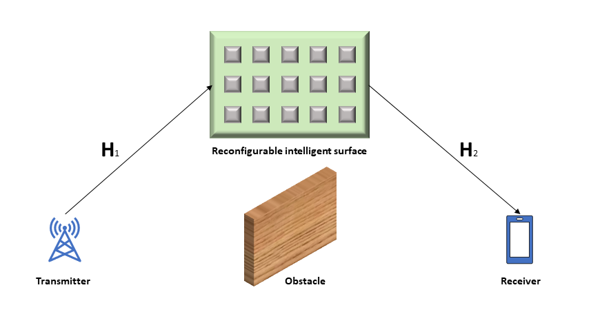
Figure 1: System Model.

We consider a RIS-assisted wireless communication system with $t$ transmit and $r$ receive antennas shown in Fig. 1. Both of the transmitter and receiver have multiple antennas which are placed as uniform linear arrays (ULAs). The direct link is blocked by an obstacle (i.e. a wall or building) which is situated between the transmit antennas and the receive antennas. A rectangular RIS of $N_{ris}$ elements is utilized to improve the whole system performance, and only reflection-type RIS is considered in this paper. We assume that all the RIS elements are ideal which means that each of them can independently influence the phase and the reflection angle of the impinging wave.

We let $m=\min\{t,r\}$. The signal vector at the receive antenna array is given by

$$\mathbf{Y}=\mathbf{H}\mathbf{X}+\mathbf{W},$$ (1)

where $\mathbf{H}\in\mathbb{C}^{r\times t}$ is the channel matrix, $\mathbf{X}\in\mathbb{C}^{t\times n}$ is the transmit signal over $n$ channel uses, $\mathbf{Y}\in\mathbb{C}^{r\times n}$ is the corresponding received signal, and $\mathbf{W}\in\mathbb{C}^{r\times n}$ is the additive noise at the receiver, which is independent of $\mathbf{H}$ and has independent and identically distributed (i.i.d.) $\mathcal{CN}(0,1)$ entries.

The channel matrix $\mathbf{H}$ of our RIS-assisted system can be expressed as

$$\mathbf{H}=\mathbf{H}_{2}\boldsymbol{\Sigma}(\boldsymbol{\theta})\mathbf{H}_{1},$$ (2)

where $\mathbf{H}_{1}\in\mathbb{C}^{N_{ris}\times t}$ represents the channel between the transmitter and the RIS, $\mathbf{H}_{2}\in\mathbb{C}^{r\times N_{ris}}$ represents the channel between the RIS and the receiver, and $\boldsymbol{\Sigma}(\boldsymbol{\theta})=diag(\boldsymbol{\theta})\in\mathbb{C}^{N_{ris}\times N_{ris}}$, where $\boldsymbol{\theta}=[\theta_{1},\dots,\theta_{N_{ris}}]^{T}\in\mathbb{C}^{N_{ris}\times 1}$ represents the signal reflecting coefficient from the RIS. In this paper, similar to the related works [33, 34, 35], we assume that the signal reflection from any RIS element is ideal, i.e., without any power loss. In other words, we may write $\theta_{i}=\exp\{j\phi_{i}\}$ for $i=1,\dots,N_{ris}$, where $\phi_{i}$ is the phase shift induced by the $i$-th RIS element, which follows the uniform distribution in $[0,2\pi)$. Equivalently, we may write

$$|\theta_{i}|=1,\quad i=1,\dots,N_{ris}.$$ (3)

Throughout this paper, we define $\lambda_{max}(\cdot)$ as a function computing the $m$ largest eigenvalues of a channel matrix, and $\mathbf{g}=[g_{1},\dots,g_{m}]^{T}$, then

$$\mathbf{g}=\lambda_{max}\big{(}\mathbf{H}^{H}\mathbf{H}\big{)},$$ (4)

where $g_{1}\geq\dots\geq g_{m}$ are the $m$ largest eigenvalues.

Let us consider input and output sets $\mathcal{A}$ and $\mathcal{B}$ and a conditional probability measure $P_{\mathbf{Y}|\mathbf{X}}\mathrel{\mathop{\ordinarycolon}}\mathcal{A}\mapsto\mathcal{B}$. We denote a codebook with $M$ codewords by $(\mathbf{C}_{1},\dots,\mathbf{C}_{M})$. A decoder which can be defined as a random transformation $P_{Z|\mathbf{Y}}\mathrel{\mathop{\ordinarycolon}}\mathcal{B}\mapsto\{1,\dots,M\}$ which satisfies

$$\frac{1}{M}\bigg{(}\sum_{i=1}^{M}P_{Z|\mathbf{X}}(i|\mathbf{C}_{i})\bigg{)}=1-\epsilon,$$ (5)

where $\epsilon$ is the average error probability. We also consider that each codeword $\mathbf{C}_{i}$ satisfies the equal power constraint $||\mathbf{C}_{i}||^{2}=nP$, where $P$ is the transmit power. Then, a codebook and a decoder whose average error probability is smaller than $\epsilon$ are termed as an $(n,M,\epsilon)$ code. In this paper, the information density also plays an essential role, which is defined as

$$i(X;Y)=\log{\frac{dP_{XY}}{d(P_{X}\times P_{Y})}(X,Y)}.$$ (6)

III Achievability Bound

In this section, our achievability bound for the examined RIS MIMO system is presented below.

Theorem 1.

We consider a communication system having the finite input alphabet $\mathcal{A}$, and the continuous output alphabet $\mathcal{B}$. Let $p(\mathbf{Y},\mathbf{H}|\mathbf{X})$ be the corresponding conditional PDF on $\mathcal{B}$ for all $\mathbf{X}\in\mathcal{A}$, where $\mathbf{H}$ is a channel matrix which is distributed according to some density functions. The input distribution $P(\mathbf{X})\overset{\triangle}{=}[\mathbf{q}_{0},\dots,\mathbf{q}_{t}]^{T}$, where $\mathbf{q}_{i}=[q_{i,0},\dots,q_{i,|\mathcal{A}|}]$ is equiprobable. Then we define the mutual information and the unconditional information variance as

$$I(X;Y)\overset{\triangle}{=}\int_{0}^{\infty}\int_{-\infty}^{\infty}\sum_{\mathbf{X}\in\mathcal{A}^{t}}\bigg{(}P(\mathbf{X})p(\mathbf{Y},\mathbf{H}|\mathbf{X})\log\big{\{}\frac{p(\mathbf{Y},\mathbf{H}|\mathbf{X})}{\sum_{\mathbf{X}^{\prime}\in\mathcal{A}^{t}}P(\mathbf{X}^{\prime})p(\mathbf{Y},\mathbf{H}|\mathbf{X}^{\prime})}\big{\}}\bigg{)}d\mathbf{Y}d\mathbf{H},$$ (7)

$$U(X;Y)\overset{\triangle}{=}\int_{0}^{\infty}\int_{-\infty}^{\infty}\sum_{\mathbf{X}\in\mathcal{A}^{t}}\bigg{(}{P}(\mathbf{X})p(\mathbf{Y},\mathbf{H}|\mathbf{X})\log^{2}\big{\{}\frac{p(\mathbf{Y},\mathbf{H}|\mathbf{X})}{\sum_{\mathbf{X}^{\prime}\in\mathcal{A}^{t}}{P}(\mathbf{X}^{\prime})p(\mathbf{Y},\mathbf{H}|\mathbf{X}^{\prime})}\big{\}}\bigg{)}d\mathbf{Y}d\mathbf{H}\\ -[I(X;Y)]^{2}.$$ (8)

Thus for the RIS MIMO channel and arbitrary $0<\epsilon<1$, we have the achievability bound

$$R\geq I(X;Y)-\sqrt{\frac{U(X;Y)}{n}}Q^{-1}(\epsilon)+\frac{1}{n}+\mathcal{O}(n^{-\frac{3}{2}}),$$ (9)

where $Q$ is the complementary Gaussian cumulative distribution function $Q(x)=\int_{x}^{\infty}\frac{1}{\sqrt{2\pi}}\\ \exp(-\frac{u^{2}}{2})du$.

The proof of Th. 1 can be found below.

Proof.

We need to introduce an important tool for proving Th. 1, that is the Berry-Esseen theorem [47].

Theorem 2.

[Berry-Esseen theorem] Let $X_{k},k=1,\dots,n$ be independent with

$$\mu_{k}=\mathbb{E}[X_{k}],\quad\sigma_{k}^{2}=Var[X_{k}],\quad t_{k}=\mathbb{E}[|X_{k}-\mu_{k}|^{3}],\quad\sigma^{2}=\sum_{k=1}^{n}\sigma_{k}^{2}\quad\textrm{and}\quad T=\sum_{k=1}^{n}t_{k}.$$

Then for any $-\infty<\tau<\infty$

$$\Big{|}\mathbb{P}\Big{[}\sum_{k=1}^{n}(X_{k}-\mu_{k})\geq\tau\sigma\Big{]}-Q(\tau)\Big{|}\leq\frac{6T}{\sigma^{3}}.$$ (10)

For the proof of Th. 1, we first need to prove that the second moment of $i(X;Y)$ is nonzero and its third moment is always less than infinite.

$$U(X;Y)=\mathbb{E}[|i(X;Y)-I(X;Y)|^{2}]$$ (11)

$$=\int_{0}^{\infty}\int_{-\infty}^{\infty}\sum_{\mathbf{X}\in\mathcal{A}^{t}}\Big{(}{P}(\mathbf{X})p(\mathbf{Y},\mathbf{H}|\mathbf{X})(1-{P}(\mathbf{X})p(\mathbf{Y},\mathbf{H}|\mathbf{X}))\log^{2}\big{\{}\frac{p(\mathbf{Y},\mathbf{H}|\mathbf{X})}{\sum_{\mathbf{X}^{\prime}\in\mathcal{A}^{t}}{P}(\mathbf{X}^{\prime})p(\mathbf{Y},\mathbf{H}|\mathbf{X}^{\prime})}\big{\}}\Big{)}$$

$$-2\binom{|\mathcal{A}|^{t}}{2}\bigg{(}{P}(\mathbf{X})p(\mathbf{Y},\mathbf{H}|\mathbf{X})\log\big{\{}\frac{p(\mathbf{Y},\mathbf{H}|\mathbf{X})}{\sum_{\mathbf{X}^{\prime}\in\mathcal{A}^{t}}{P}(\mathbf{X}^{\prime})p(\mathbf{Y},\mathbf{H}|\mathbf{X}^{\prime})}\big{\}}\bigg{)}^{2}d\mathbf{Y}d\mathbf{H}$$

$$=\int_{0}^{\infty}\int_{-\infty}^{\infty}\sum_{\mathbf{X}\in\mathcal{A}^{t}}\bigg{(}{P}(\mathbf{X})p(\mathbf{Y},\mathbf{H}|\mathbf{X})(1-p(\mathbf{Y},\mathbf{H}|\mathbf{X}))$$ (12)

$$\quad\log^{2}\big{\{}\frac{p(\mathbf{Y},\mathbf{H}|\mathbf{X})}{\sum_{\mathbf{X}^{\prime}\in\mathcal{A}^{t}}{P}(\mathbf{X}^{\prime})p(\mathbf{Y},\mathbf{H}|\mathbf{X}^{\prime})}\big{\}}\bigg{)}d\mathbf{Y}d\mathbf{H}$$

$$>0,$$ (13)

where (12) follows from $2\binom{|\mathcal{A}|^{t}}{2}/|\mathbb{A}|^{t}=|\mathcal{A}|^{t}-1$ and ${P}(\mathbf{X})=1/|\mathcal{A}|^{t}$ and (13) follows from $1-p(\mathbf{Y},\mathbf{H}|\mathbf{X})>0$.

Then, we need to show the third moment is less than infinite.

$$T(X;Y)=\mathbb{E}[|i(X;Y)-I(X;Y)|^{3}]$$ (14)

$$=\Big{|}\mathbb{E}[|i(X;Y)|^{3}]+3I(X;Y)^{2}\mathbb{E}[|i(X;Y)|]-3I(X;Y)\mathbb{E}[|i(X;Y)|^{2}]-I(X;Y)^{3}\Big{|}$$ (15)

$$=\Big{|}\mathbb{E}[|i(X;Y)|^{3}]-3I(X;Y)\mathbb{E}[|i(X;Y)|^{2}]+2I(X;Y)^{3}\Big{|}$$ (16)

$$\leq\mathbb{E}[|i(X;Y)|^{3}]+2I(X;Y)^{3}$$ (17)

$$\leq\mathbb{E}[|p(\mathbf{Y},\mathbf{H}|\mathbf{X})|^{3}]+\mathbb{E}[|\frac{1}{\sum_{\mathbf{X}^{\prime}\in\mathcal{A}^{t}}{P}(\mathbf{X}^{\prime})p(\mathbf{Y},\mathbf{H}|\mathbf{X}^{\prime})}|^{3}]+2I(X;Y)^{3}$$ (18)

$$\leq|\mathcal{B}|(3e^{-1}\log{e})^{3}+2I(X;Y)^{3},$$ (19)

where (18) follows from Holder’s inequality and (19) follows from $\max_{0<x<1}\{x\log^{3}{x}\}=0$ at $x=1$ and $\max_{0<x<1}\{x\log^{3}{\frac{1}{x}}\}=(3e^{-1}\log{e})^{3}$ at $x=e^{-3}$. We denote $i(X^{n};Y^{n})=\sum_{n}i(X;Y)$, and let its second moment $\sum_{n}U(X;Y)$ be nonzero and its third moment $\\ \sum_{n}\mathbb{E}[|i(X;Y)-I(X;Y)|^{3}]<\infty$. Thus, Th.2 is still applicable to $i(X^{n};Y^{n})$.

According to the DT bound in [32], $\epsilon\leq\mathbb{E}\big{[}\exp\big{\{}-[i(X^{n};Y^{n})-\log\frac{M-1}{2})]^{+}\big{\}}\big{]}$, where $[\cdot]^{+}$ denotes $\max\{\cdot,0\}$. In the sequel, we prove that there exist some $\lambda$ values, so that

$$\epsilon \geq\mathbb{E}\Big{[}\exp\{0\}1_{\{i(X^{n};Y^{n})-\log{\lambda}\leq 0\}}\Big{]}+\mathbb{E}\Big{[}\exp\big{\{}-i(X^{n};Y^{n})+\log\lambda\big{\}}1_{\{i(X^{n};Y^{n})-\log{\lambda}>0\}}\Big{]}$$

$$=\mathbb{P}\bigg{[}i(X^{n};Y^{n})\leq\log{\lambda}\bigg{]}+\lambda\mathbb{E}\bigg{[}\exp\big{\{}-i(X^{n};Y^{n})\big{\}}1_{\{i(X^{n};Y^{n})>\log{\lambda}\}}\bigg{]}.$$ (20)

The first step is to obtain the upper bound of the first part of the right-hand side of (20). After applying Th. 2, we have

$$\mathbb{P}\bigg{[}i(X^{n};Y^{n})\leq nI(X;Y)-\tau\sqrt{nU(X;Y)}\bigg{]}\leq\frac{6T(X;Y)}{\sqrt{n}U(X;Y)^{\frac{3}{2}}}+Q(\tau).$$ (21)

We assume

$$\log\lambda=nI(X;Y)-\tau\sqrt{nU(X;Y)},$$ (22)

and

$$\mathbb{P}\bigg{[}i(X^{n};Y^{n})\leq\log{\lambda}\bigg{]}\leq\frac{6T(X;Y)}{\sqrt{n}U(X;Y)^{\frac{3}{2}}}+Q(\tau).$$ (23)

The upper bound of the second part of the right-hand side of (20) is given below. For $0\leq i<\infty$ and any $\Delta>0$,

$$\mathbb{P}\Big{[}-\sqrt{nU(X;Y)}(\tau-\frac{i\Delta}{\sqrt{nU(X;Y)}})\leq i(X^{n};Y^{n})$$ (24)

$$\qquad\qquad\qquad\qquad\qquad-nI(X;Y)\leq-\sqrt{nU(X;Y)}(\tau-\frac{(i+1)\Delta}{\sqrt{nU(X;Y)}})\Big{]}$$

$$=\mathbb{P}\Big{[}\log\lambda+i\Delta\leq i(X^{n};Y^{n})\leq\log\lambda+(i+1)\Delta\Big{]}$$ (25)

$$\leq\frac{12T(X;Y)}{\sqrt{n}U(X;Y)^{\frac{3}{2}}}+Q(\tau+\frac{i\Delta}{\sqrt{nU(X;Y)}})-Q(\tau+\frac{(i+1)\Delta}{\sqrt{nU(X;Y)}}),$$ (26)

where (III) is obtained by applying Th. 2 twice. Then,

$$\mathbb{E}\bigg{[}\exp\big{\{}-i(X^{n};Y^{n})\big{\}}1_{\{i(X^{n};Y^{n})>\log{\lambda}\}}\bigg{]}$$ (27)

$$=\sum_{i=0}^{\infty}\exp\{-(\log{\lambda}+i\Delta)\}\mathbb{P}\bigg{[}\log{\lambda}+i\Delta\leq i(X^{n};Y^{n})\leq\log{\lambda}+(i+1)\Delta\bigg{]}$$ (28)

$$\leq\sum_{i=0}^{\infty}\exp\{-(\log{\lambda}+i\Delta)\}\bigg{[}\frac{12T(X;Y)}{\sqrt{n}U(X;Y)^{\frac{3}{2}}}+Q(\tau+\frac{i\Delta}{\sqrt{nU(X;Y)}})-Q(\tau+\frac{(i+1)\Delta}{\sqrt{nU(X;Y)}})\bigg{]}$$ (29)

$$\leq\bigg{(}\frac{\Delta}{\sqrt{2\pi}\sqrt{nU(X;Y)}}+\frac{12T(X;Y)}{\sqrt{n}U(X;Y)^{\frac{3}{2}}}\bigg{)}\sum_{i=0}^{\infty}\exp\{-(\log{\lambda}+i\Delta)\},$$ (30)

where (28) is a result of the Riemann integral and (30) follows from the fact that for any $\sigma$, $Q(\frac{x}{\sigma})-Q(\frac{x+\Delta}{\sigma})\leq\frac{\Delta}{\sqrt{2\pi}\sigma}$. Thus, we have

$$\lambda\mathbb{E}\bigg{[}\exp\big{\{}-i(X^{n};Y^{n})\big{\}}1_{\{i(X^{n};Y^{n})>\log{\lambda}\}}\bigg{]}$$ (31)

$$\leq\lambda\bigg{(}\frac{\Delta}{\sqrt{2\pi}\sqrt{nU(X;Y)}}+\frac{12T(X;Y)}{\sqrt{n}U(X;Y)^{\frac{3}{2}}}\bigg{)}\sum_{i=0}^{\infty}\exp\{-(\log{\lambda}+i\Delta)\}$$ (32)

$$=\bigg{(}\frac{\Delta}{\sqrt{2\pi}\sqrt{nU(X;Y)}}+\frac{12T(X;Y)}{\sqrt{n}U(X;Y)^{\frac{3}{2}}}\bigg{)}\sum_{i=0}^{\infty}\exp\{-i\Delta\}$$ (33)

$$=\bigg{(}\frac{\Delta}{\sqrt{2\pi}\sqrt{nU(X;Y)}}+\frac{12T(X;Y)}{\sqrt{n}U(X;Y)^{\frac{3}{2}}}\bigg{)}\frac{\exp\{\Delta\}}{\exp\{\Delta\}-1},$$ (34)

where (34) follows for any $\exp\{x\}>1$, $\sum_{i=0}^{\infty}\exp\{-ix\}=\frac{\exp\{x\}}{\exp\{x\}-1}$. Substituting (23) and (34) into (20), we have

$$\mathbb{P}\bigg{[}i(X^{n};Y^{n})\leq\log{\lambda}\bigg{]}+\lambda\mathbb{E}\bigg{[}\exp\big{\{}-i(X^{n};Y^{n})\big{\}}1_{\{i(X^{n};Y^{n})>\log{\lambda}\}}\bigg{]}\\ \leq Q(\tau)+\frac{1}{\sqrt{n}}\frac{6T(X;Y)}{U(X;Y)^{\frac{3}{2}}}\Big{(}1+2\frac{\exp\{\Delta\}}{\exp\{\Delta\}-1}+\frac{U(X;Y)\Delta\exp\{\Delta\}}{\sqrt{2\pi}6T(X;Y)(\exp\{\Delta\}-1)}\Big{)}.$$ (35)

Based on (20), we can assume that the right hand side of (35) equals to $\epsilon$, then we obtain the value of $\tau$

$$\tau=Q^{-1}\Big{(}\epsilon-\frac{1}{\sqrt{n}}\frac{6T(X;Y)}{U(X;Y)^{\frac{3}{2}}}\Big{(}1+2\frac{\exp\{\Delta\}}{\exp\{\Delta\}-1}+\frac{U(X;Y)\Delta\exp\{\Delta\}}{\sqrt{2\pi}6T(X;Y)(\exp\{\Delta\}-1)}\Big{)}\Big{)}.$$ (36)

For large $n$, the second item inside the Q function of (36) vanishes. Therefore, we can obtain $\tau=Q^{-1}(\epsilon)+\mathcal{O}(\frac{1}{\sqrt{n}})$. Then, we have $\log\lambda=nI(X;Y)-Q^{-1}(\epsilon)\sqrt{nU(X;Y)}+\mathcal{O}(\frac{1}{\sqrt{n}})$.

Thus,

$$\log\frac{M-1}{2}\geq\log\lambda=nI(X;Y)-Q^{-1}(\epsilon)\sqrt{nU(X;Y)}+\mathcal{O}(\frac{1}{\sqrt{n}})$$ (37)

$$R\geq I(X;Y)-Q^{-1}(\epsilon)\sqrt{\frac{U(X;Y)}{n}}+\frac{1}{n}+\mathcal{O}(n^{-\frac{3}{2}}).$$ (38)

∎

To accomplish the achievability bound by applying Th. 1, we need to obtain the exact expression of both (7) and (8). At first, for our system model, the input distribution $P(\mathbf{X})=[\mathbf{q}_{0},\dots,\mathbf{q}_{t}]^{T}$, where $\mathbf{q}_{i}=[\frac{1}{2},\frac{1}{2}]$ and $\mathbf{q}_{i}=[\frac{1}{4},\frac{1}{4},\frac{1}{4},\frac{1}{4}]$, for BPSK and QPSK respectively. And the conditional PDF of a MIMO Rayleigh fading channel, $p(\mathbf{Y},\mathbf{H}|\mathbf{X})$, is given by [45][46]

$$p(\mathbf{Y},\mathbf{H}|\mathbf{X})=p(\mathbf{H})p(\mathbf{Y}|\mathbf{X},\mathbf{H})=\frac{p(\mathbf{H})}{det(\pi\mathbf{I}_{r})}\exp\big{(}-(\mathbf{Y}-\mathbf{X}\mathbf{H})^{H}(\mathbf{Y}-\mathbf{X}\mathbf{H})\big{)},$$ (39)

where $\mathbf{I}_{r}$ designates the $r\times r$ identity matrix and $det(\cdot)$ denotes the determinant.

Then

$$I(X;Y) =\int_{0}^{\infty}\int_{-\infty}^{\infty}\sum_{\mathbf{X}\in\mathcal{A}^{t}}\bigg{(}P(\mathbf{X})p(\mathbf{Y},\mathbf{H}|\mathbf{X})\log\big{\{}\frac{p(\mathbf{Y},\mathbf{H}|\mathbf{X})}{\sum_{\mathbf{X}^{\prime}\in\mathcal{A}^{t}}P(\mathbf{X}^{\prime})p(\mathbf{Y},\mathbf{H}|\mathbf{X}^{\prime})}\big{\}}\bigg{)}d\mathbf{Y}d\mathbf{H}$$ (40)

$$=\sum_{\mathbf{X}\in\mathcal{A}^{t}}\frac{q_{\mathbf{X}}}{det(\pi\mathbf{I}_{r})}\underbrace{\int_{0}^{\infty}\cdots\int_{0}^{\infty}}_{\begin{subarray}{c}\text{m-dimensions}\\ \text{(w.r.t. $\mathbf{h}$)}\end{subarray}}\underbrace{\int_{-\infty}^{\infty}\cdots\int_{-\infty}^{\infty}}_{\begin{subarray}{c}\text{m-dimensions}\\ \text{(w.r.t. $\mathbf{y}$)}\end{subarray}}\prod_{i=0}^{m-1}p(\mathbf{h}_{i})\exp\{-\frac{1}{2}||\mathbf{y}_{i}-\mathbf{h}_{i}\mathbf{x}_{i}||^{2}\}$$ (41)

$$\bigg{(}-\log e\sum_{j=0}^{m-1}\frac{1}{2}||\mathbf{y}_{j}-\mathbf{h}_{j}\mathbf{x}_{j}||^{2}-\log\big{\{}\sum_{k=0}^{m-1}\sum_{\mathbf{x}_{k}^{\prime}\in\mathcal{A}}\mathbf{q}_{k}\exp\{-\frac{1}{2}||\mathbf{y}_{k}-\mathbf{h}_{k}\mathbf{x}^{\prime}_{k}||^{2}\}\big{\}}\bigg{)}d\mathbf{y}d\mathbf{h}.$$

and

$$U(X;Y) =\int_{0}^{\infty}\int_{-\infty}^{\infty}\sum_{\mathbf{X}\in\mathcal{A}^{t}}\bigg{(}P(\mathbf{X})p(\mathbf{Y},\mathbf{H}|\mathbf{X})\log\big{\{}\frac{p(\mathbf{Y},\mathbf{H}|\mathbf{X})}{\sum_{\mathbf{X}^{\prime}\in\mathcal{A}^{t}}P(\mathbf{X}^{\prime})p(\mathbf{Y},\mathbf{H}|\mathbf{X}^{\prime})}\big{\}}\bigg{)}d\mathbf{Y}d\mathbf{H}$$ (42)

$$=\sum_{\mathbf{X}\in\mathcal{A}^{t}}\frac{q_{\mathbf{X}}}{det(\pi\mathbf{I}_{r})}\underbrace{\int_{0}^{\infty}\cdots\int_{0}^{\infty}}_{\begin{subarray}{c}\text{m-dimensions}\\ \text{(w.r.t. $\mathbf{h}$)}\end{subarray}}\underbrace{\int_{-\infty}^{\infty}\cdots\int_{-\infty}^{\infty}}_{\begin{subarray}{c}\text{m-dimensions}\\ \text{(w.r.t. $\mathbf{y}$)}\end{subarray}}\prod_{i=0}^{m-1}p(\mathbf{h}_{i})\exp\{-\frac{1}{2}||\mathbf{y}_{i}-\mathbf{h}_{i}\mathbf{x}_{i}||^{2}\}$$ (43)

$$\bigg{(}-\log e\sum_{j=0}^{m-1}\frac{1}{2}||\mathbf{y}_{j}-\mathbf{h}_{j}\mathbf{x}_{j}||^{2}-\log\big{\{}\sum_{k=0}^{m-1}\sum_{\mathbf{x}_{k}^{\prime}\in\mathcal{A}}\mathbf{q}_{k}\exp\{-\frac{1}{2}||\mathbf{y}_{k}-\mathbf{h}_{k}\mathbf{x}^{\prime}_{k}||^{2}\}\big{\}}\bigg{)}d\mathbf{y}d\mathbf{h}$$

$$-[I(X;Y)]^{2}.$$

Next, we need to find the expression of $p(\mathbf{h}_{i})$. According to (2), $p(\mathbf{h}_{i})$ follows the Rayleigh distribution when $N_{ris}$ is sufficiently large. Thus,

$$p(\mathbf{h}_{i})=\frac{2\mathbf{h}_{i}}{N_{ris}}\exp\{-\frac{\mathbf{h}^{2}_{i}}{N_{ris}}\}.$$ (44)

Therefore, we can combine (41), (43) and (44) together, and put the results into Th. 1, then we can finally derive our achievability bound.

IV Converse Bound

In this section, we derive the converse bound for the investigated RIS MIMO system on the basis of the meta-converse theorem [32] under the assumption of each codeword having an equal power.

Theorem 3.

We consider the same equiprobable input distribution $P(\mathbf{X})$ and the same mutual information and unconditional information variance as defined in (7) and (8), respectively, the converse bound for the RIS MIMO channel and arbitrary $0<\epsilon<1$ is given by,

$$R\leq{I(X;Y)}-\sqrt{\frac{{U(X;Y)}}{n}}Q^{-1}(\epsilon+\frac{\epsilon}{\sqrt{n}})+\frac{(m+1)\log n}{2n}+\mathcal{O}(n^{-\frac{3}{2}}).$$ (45)

The proof of (45) can be found below.

Proof.

We assume the transmitter is not aware of the realizations of the channel matrix $\mathbf{H}$. We denote the average power constraint

$$\mathbf{p}(\mathbf{X})\overset{\Delta}{=}\frac{1}{n}\mathbf{X}\mathbf{X}^{H}.$$ (46)

Based on [38, 39, 40], to evaluate the converse bound of an auxiliary channel, we need to obtain the lower bound of $\epsilon^{\prime}$, which is the average error probability over the corresponding auxiliary channel. We thus denote the auxiliary channel $Q$ as:

$$Q_{\mathbf{Y}|\mathbf{X},\mathbf{H}}\overset{\Delta}{=}\prod_{j=1}^{n}Q_{Y_{j}|\mathbf{X},\mathbf{H}},$$ (47)

where

$$Q_{Y_{j}|\mathbf{X},\mathbf{H}}=\mathcal{CN}(0,\mathbf{I}_{r}+\mathbf{H}\mathbf{p}(\mathbf{X})\mathbf{H}^{H}),$$ (48)

We denote $\mathbf{B}\overset{\Delta}{=}\mathbf{I}_{r}+\mathbf{H}\mathbf{p}(\mathbf{X})\mathbf{H}^{H}$ and let its eigenvector $\boldsymbol{\omega}=[\omega_{1},\dots,\omega_{m}]=\lambda_{max}\big{(}\mathbf{B})$. Note that $\mathbf{P}=\mathbf{p}(\mathbf{X})$ is the only factor that affects the output of the $Q_{\mathbf{Y}|\mathbf{X},\mathbf{H}}$ channel. Let the space $\mathbf{S}\overset{\Delta}{=}\mathbf{p}(\mathbf{Y})=\frac{1}{n}\mathbf{Y}\mathbf{Y}^{H}$ and its entry is defined as the square of the norm of $\mathbf{Y}$ and is then normalized by the blocklength $n$, which is shown below

$${S}_{j}=\frac{\omega_{j}}{n}\sum_{i=1}^{n}|Z_{j,i}|^{2},\quad j=1,\dots,m,$$ (49)

where $Z_{j,i}\sim\mathcal{CN}(0,1)$. $\mathbf{S}$ can be seen as the statistical expression of the receiver’s detection of $\mathbf{X}$ from $(\mathbf{Y},\mathbf{H})$. Thus the auxiliary channel $Q_{\mathbf{Y}|\mathbf{X},\mathbf{H}}$ can be seen as $Q_{\mathbf{S}|\mathbf{B}}$. From (49), we note that the $S_{j}$ follows the Gamma distribution, and its corresponding PDF is given by

$$q_{S_{j}|B_{j}}(s_{j}|\omega_{j})=\frac{n^{n}}{(\omega_{j})^{n}\Gamma(n)}s_{j}^{n-1}\exp\Big{\{}-\frac{ns_{j}}{\omega_{j}}\Big{\}}.$$ (50)

Moreover, as $Q_{\mathbf{S}|\mathbf{B}}$ is a product of $m$ copies of the PDF of $S_{j}$. We can obtain the PDF of $Q_{\mathbf{S}|\mathbf{B}}$ by the theorem shown below[44].

Theorem 4.

Given $N$ independent Gamma-distributed random variables $x_{i}$ and that their shape parameter $k$ and scale parameter $\theta$ are all the same, we have the PDF of $x_{i}$ as

$$f_{i}(x_{i})=\frac{1}{\Gamma(k)\theta^{k}}x_{i}^{k-1}e^{-\frac{x_{i}}{\theta}}.$$ (51)

We denote $z$ as the product of $N$ independent gamma variables $x_{i}$. Therefore, the PDF of $z=x_{1}x_{2}\dots x_{N}$ is a normalized Meijer G-function as

$$g(z)=\mathcal{K}G^{\,N,0}_{0,N}\big{\lparen}\begin{smallmatrix}\\ k-1\end{smallmatrix}\big{|}\,\frac{z}{\theta^{N}}\big{\rparen},$$ (52)

where $\mathcal{K}$ is a normalizing factor which is

$$\mathcal{K}=(\frac{1}{\theta})^{N}\prod_{i=1}^{N}\frac{1}{\Gamma(k)},$$ (53)

and

$$G^{\,m,n}_{p,q}\big{\lparen}\begin{smallmatrix}j_{1},j_{2},\dots,j_{p}\\ k_{1},k_{2},\dots,k_{q}\end{smallmatrix}\big{|}\,z\big{\rparen}=\frac{1}{2\pi i}\int_{c-i^{\infty}}^{c+i^{\infty}}z^{-s}\cdot\frac{\prod_{j=1}^{m}\Gamma(s+k_{j})\cdot\prod_{j=1}^{n}\Gamma(1-j_{j}-s)}{\prod_{j=n+1}^{p}\Gamma(s+j_{j})\cdot\prod_{j=m+1}^{q}\Gamma(1-k_{j}-s)}ds,$$ (54)

where $c$ is a vertical contour in the complex plane chosen to separate the poles of $\Gamma(s+k_{j})$ from those of $\Gamma(1-j_{k})-s$.

The proof of Th. 4 can be found in Appendix A.

We set two parameters, the shape parameter $k=n$ and the scale parameter $\theta_{j}=\frac{\omega_{j}}{n}$. The number of copies in our case is $N=m$. Then we can apply Th. 4 to calculate the PDF of $Q_{\mathbf{S}|\mathbf{B}}$ as

$$q_{S_{j}|B_{j}}(s_{j}|\omega_{j})=\mathcal{K}G^{\,m,0}_{0,m}\big{\lparen}\begin{smallmatrix}\\ n-1\end{smallmatrix}\big{|}\,s_{j}(\frac{n}{\omega_{j}})^{m}\big{\rparen},$$ (55)

where

$$\mathcal{K}=(\frac{n}{\omega_{j}})^{m}\prod_{i=1}^{m}\frac{1}{\Gamma(n)},$$ (56)

and

$$G^{\,m,0}_{0,m}\big{\lparen}\begin{smallmatrix}\\ n-1\end{smallmatrix}\big{|}\,s_{j}(\frac{n}{\omega_{j}})^{m}\big{\rparen}=\frac{1}{2\pi i}\int_{c-i^{\infty}}^{c+i^{\infty}}(s_{j}(\frac{n}{1+\omega_{j}})^{m})^{-z}\prod_{j=1}^{m}\Gamma(z+n-1)dz.$$ (57)

Consider an arbitrary code for the auxiliary channel $Q$. The decoding sets corresponding to the $M$ codewords is denoted by $D_{i},i=1,...,M$. $\epsilon^{\prime}$ is the average error probability over the auxiliary channel $Q$. Then we have

$$1-\epsilon^{\prime} =\frac{1}{M}\mathbb{E}_{\mathbf{H}}\bigg{[}\sum_{i=0}^{M}\int_{D_{i}}q_{\mathbf{S}|\mathbf{B}}(\mathbf{s})d\mathbf{s}\bigg{]}$$ (58)

$$\leq\mathbb{E}_{\mathbf{H}}\bigg{[}\int_{D_{0}}q_{\mathbf{S}|\mathbf{B}}(\mathbf{s})d\mathbf{s}\bigg{]}$$ (59)

$$\leq\mathbb{E}_{\mathbf{H}}\bigg{[}\max\{q_{\mathbf{S}|\mathbf{B}}(\mathbf{s})\}\times Leb(D_{0})\bigg{]}.$$ (60)

Next we need to provide the upper bound of the output space of an arbitrary decoding set, $Leb(D_{0})$. Due to the power allocation vector $\mathbf{p}(\mathbf{X})$, the space $\mathbf{P}$ can be bounded by a certain ball in $\mathbb{R}^{m}$. Based on the definition of $\mathbf{S}$, its space is a slightly larger ball than the space $\mathbf{P}$. Thus we can obtain the upper bounded Lebesgue measure [41] of $D_{0}$,

$$Leb(D_{0})\leq Leb(\mathbf{S})\leq\frac{K}{M},$$ (61)

where $Leb$ is the Lebesgue measure and $K$ is a constant.

Then the decoding set of any codeword has a Lebesgue measure space which is always smaller than $\frac{K}{M}$. Therefore, we have

$$1-\epsilon^{\prime} \leq\mathbb{E}_{\mathbf{H}}\bigg{[}\max\{q_{\mathbf{S}|\mathbf{B}}(\mathbf{s})\}\times\frac{K}{M}\bigg{]}$$ (62)

$$\leq\frac{1}{M}\bigg{(}\frac{(n-1)^{n}\exp\{-(n-1)\}}{\Gamma(n)}\bigg{)}^{m}\mathbb{E}_{\mathbf{H}}\bigg{[}\prod_{i=1}^{m}\omega_{j}\bigg{]}$$ (63)

$$=\frac{1}{M}\bigg{(}\frac{(n-1)^{n}\exp\{-(n-1)\}}{\Gamma(n)}\bigg{)}^{m}\times\int_{0}^{\infty}\prod_{i=1}^{m}(\omega_{j})p(g)dg$$ (64)

$$\leq\frac{n^{m/2}}{M}.$$ (65)

According to the binary hypothesis testing in [32], we have

$$\Lambda(\epsilon) \geq\frac{1}{\lambda}\Big{(}\epsilon-\mathbb{P}\big{[}i(X^{n};Y^{n})\leq\log{\lambda}\big{]}\Big{)}$$ (66)

$$\geq\frac{1}{\lambda}\Big{(}\epsilon-\frac{6T(X;Y)}{\sqrt{n}U(X;Y)^{\frac{3}{2}}}-Q(\tau)\Big{)},$$ (67)

where $\Lambda(\epsilon)$ denotes the average probability of error under $P_{\mathbf{Y}|\mathbf{X},\mathbf{H}}$ if the probability of error under $Q_{\mathbf{Y}|\mathbf{X},\mathbf{H}}$ is $\epsilon$ and (67) follows from (23). Then,

$$\log\Lambda(\epsilon) \geq-\log\lambda+\log\Big{(}\epsilon-\frac{6T(X;Y)}{\sqrt{n}U(X;Y)^{\frac{3}{2}}}-Q(\tau)\Big{)}$$ (68)

$$=-n{I(X;Y)}+\tau\sqrt{n{U(X;Y)}}+\log\Big{(}\epsilon-\frac{6T(X;Y)}{\sqrt{n}U(X;Y)^{\frac{3}{2}}}-Q(\tau)\Big{)},$$ (69)

where (69) follows from (22). We assume $\tau=Q^{-1}(\epsilon(1+\frac{1}{\sqrt{n}})-\frac{6T(X;Y)}{\sqrt{n}U(X;Y)^{\frac{3}{2}}})$. Thus,

$$\log\Lambda(\epsilon)\geq-n{I(X;Y)}+\sqrt{n{U(X;Y)}}Q^{-1}(\epsilon(1+\frac{1}{\sqrt{n}})-\frac{6T(X;Y)}{\sqrt{n}U(X;Y)^{\frac{3}{2}}})-\frac{1}{2}\log n.$$ (70)

Due to the fact that $\log\Lambda(\epsilon)\leq 1-\epsilon^{\prime}$, we have

$$-n{I(X;Y)}+\sqrt{n{U(X;Y)}}Q^{-1}(\epsilon+\frac{\epsilon}{\sqrt{n}})-\frac{1}{2}\log n+\mathcal{O}(\frac{1}{\sqrt{n}})\leq 1-\epsilon^{\prime}.$$ (71)

Thus substituting (71) into (65), we have

$$R\leq{I(X;Y)}-\sqrt{\frac{U(X;Y)}{n}}Q^{-1}(\epsilon+\frac{\epsilon}{\sqrt{n}})+\frac{(m+1)\log n}{2n}+\mathcal{O}(n^{-\frac{3}{2}})$$ (72)

This completes the proof.

∎

In order to complete the converse bound by applying Th. 3, we use the same input distribution as in Section III. Then after we obtain the exact expression of $p(\mathbf{Y},\mathbf{H}|\mathbf{X})$ and $p(\mathbf{h}_{i})$, we can combine (41), (43) and (44) together, and put the results into Th. 3, then we can finally derive the converse bound.

To compare with our result, we calculate the capacity of the channel whose input is a circularly symmetric complex Gaussian with zero mean and covariance $\frac{P}{t}\mathbf{I}_{t}$. The Theorem is shown below.

Theorem 5.

[36] Under the power constraint $P$, we assume the same channel with the same number of transmitting and receiving antennas as our system model. Its capacity, as determined by the complex Gaussian input, is equal to

$$\mathbb{E}_{\mathbf{g}}[\log(1+\frac{P}{t}g)]=\int_{0}^{\infty}\log(1+\frac{P}{t}g)dg,$$ (73)

where according to (4) in Section II,

$$p(g)=\sum_{i=0}^{m}\frac{i!}{2(i+\max\{r,t\}-m)!}(L_{i}^{\max\{r,t\}-m}(g/N_{ris}))^{2}(g/N_{ris})^{\max\{r,t\}-m}\exp{(-g/N_{ris})}.$$ (74)

Thus

$$C_{Gaussian}=\int_{0}^{\infty}\log(1+\frac{P}{t}g)\sum_{i=0}^{m}\frac{i!}{2(i+\max\{r,t\}-m)!}(L_{i}^{\max\{r,t\}-m}(g/N_{ris}))^{2}\\ \times(g/N_{ris})^{\max\{r,t\}-m}\exp{(-g/N_{ris})}dg.$$ (75)

V Numerical Results

V-A Evaluation of the Derived Bounds

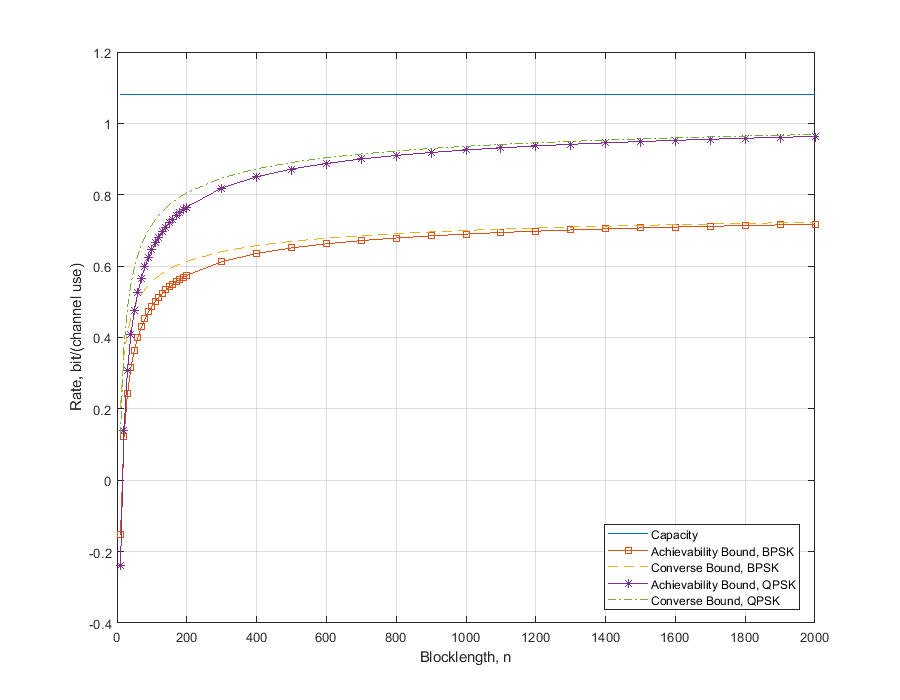
Figure 2: Achievability and converse bounds for $(n,M,\epsilon)$ codes for a RIS MIMO system over a Rayleigh fading channel and transmit antennas $t=2$ and receive antennas $r=1$, SNR=$-5$dB, $\epsilon=10^{-3}$, $N_{ris}=4$ and with BPSK and QPSK modulation, repectively.

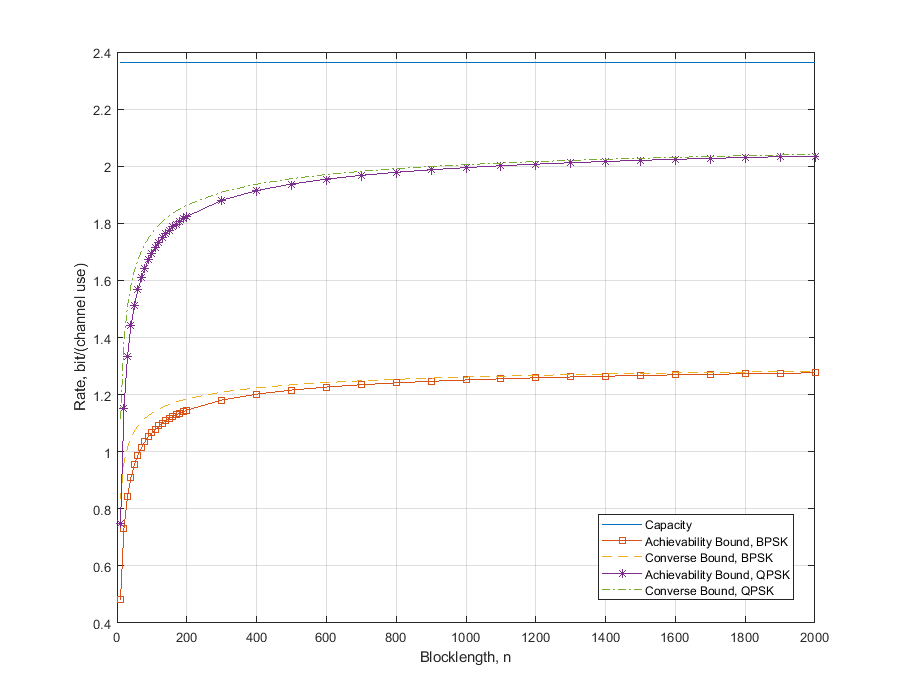
Figure 3: Achievability and converse bounds for $(n,M,\epsilon)$ codes for a RIS MIMO system over a Rayleigh fading channel and transmit antennas $t=2$ and receive antennas $r=1$, SNR=$-5$dB, $\epsilon=10^{-3}$, $N_{ris}=16$ and with BPSK and QPSK modulation, repectively.

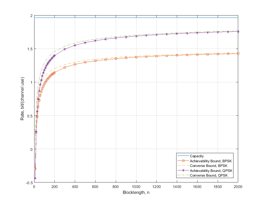
Figure 4: Achievability and converse bounds for $(n,M,\epsilon)$ codes for a RIS MIMO system over a Rayleigh fading channel and transmit antennas $t=2$ and receive antennas $r=2$, SNR=$-5$dB, $\epsilon=10^{-3}$, $N_{ris}=4$ and with BPSK and QPSK modulation, repectively.

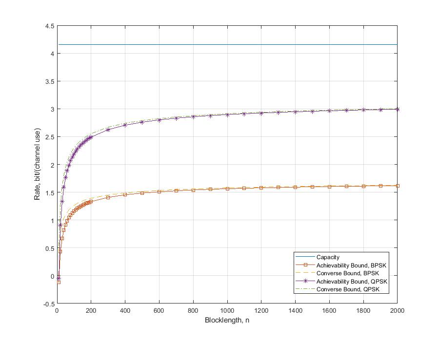
Figure 5: Achievability and converse bounds for $(n,M,\epsilon)$ codes for a RIS MIMO system over a Rayleigh fading channel and transmit antennas $t=2$ and receive antennas $r=2$, SNR=$-5$dB, $\epsilon=10^{-3}$, $N_{ris}=16$ and with BPSK and QPSK modulation, repectively.

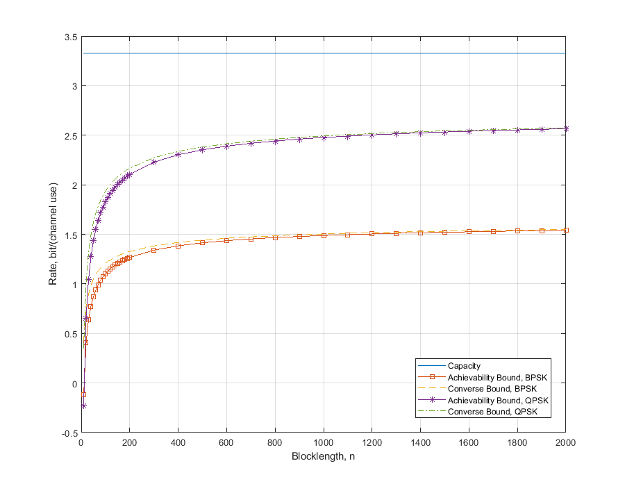
Figure 6: Achievability and converse bounds for $(n,M,\epsilon)$ codes for a RIS MIMO system over a Rayleigh fading channel and transmit antennas $t=2$ and receive antennas $r=2$, SNR=$-10$dB, $\epsilon=10^{-3}$, $N_{ris}=32$ and with BPSK and QPSK modulation, repectively.

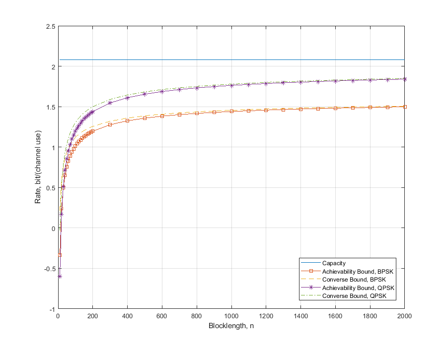
Figure 7: Achievability and converse bounds for $(n,M,\epsilon)$ codes for a RIS MIMO system over a Rayleigh fading channel and transmit antennas $t=3$ and receive antennas $r=2$, SNR=$-5$dB, $\epsilon=10^{-3}$, $N_{ris}=4$ and with BPSK and QPSK modulation, repectively.

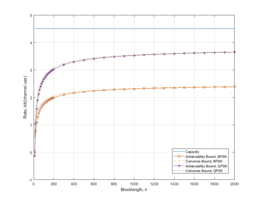
Figure 8: Achievability and converse bounds for $(n,M,\epsilon)$ codes for a RIS MIMO system over a Rayleigh fading channel and transmit antennas $t=3$ and receive antennas $r=2$, SNR=$-5$dB, $\epsilon=10^{-3}$, $N_{ris}=16$ and with BPSK and QPSK modulation, repectively.

In this section, we consider a RIS MIMO system consisting of a transmitter with multiple transmitter antennas, a rectangular RIS of $N_{ris}$ elements and a receiver with multiple receive antennas. We assume all the channels, i.e., the channels between the transmitter and the RIS, the RIS and the receiver, the transmitter and the receiver, are independent with average error probability $\epsilon=10^{-3}$. Fig. 2 shows the numerical results of the derived bounds with BPSK modulated and QPSK modulated signals and the capacity by assuming that all the channels are Rayleigh distributed, the numbers of transmit antennas and receive antennas are $t=2$, $r=1$, respectively and SNR=$-5$dB $N_{ris}=4$. From Fig. 2, we can see that $C_{Gaussian}=1.0811$ bit/(channel use), and the maximal achievable rate for BPSK modulation, which is calculated from (7), is $0.7834$ bit/(channel use) and the blocklength $n$ required to achieve above $70\%$ and $80\%$ of its maximal achievable rate starts at $n=160$ and $n=360$, respectively. The gap between the capacity and its maximal achievable rate is $0.2977$ bit/(channel use). With the QPSK modulation, the maximal achievable rate, which is also obtained from (7), is $1.0547$ bit/(channel use), and the blocklength $n$ required to achieve above $70\%$, and $80\%$ of its maximal achievable rate starts at $n=170$ and $n=380$, respectively. The gap in the QPSK case is $0.0264$ bit/(channel use).

In Fig. 3, we only change the RIS element from $N_{ris}=4$ to $N_{ris}=16$ and the rest parameters remain the same. The capacity, in this case, is $2.3629$ bit/(channel use). BPSK modulation’s maximal achievable rate is $1.3367$ bit/(channel use). The blocklength $n$, which can surpass $70\%$ and $80\%$ of its maximal achievable rate, decreases dramatically to $50$ and $100$ compared with the case of $N_{ris}=4$. For $90\%$ of its maximal achievable rate, the required blocklength $n$ is $n=410$. Moreover, the gap increases to $1.0262$ bit/(channel use). For QPSK modulation, its maximal achievable rate is $2.1338$ bit/(channel use) and the blocklength $n=110$, and $n=420$ is required to achieve above $80\%$ and $90\%$ of its maximal achievable rate. The gap also enlarges from $0.0264$ bit/(channel use) to $0.2291$ bit/(channel use). From Fig. 2 and 3, we can conclude that: 1) as $N_{ris}$ increases, the overall channel between the transmitter and the receiver becomes better. That means that the gap between the maximal achievable rate for different modulation schemes and the capacity increases and vice versa at the same SNR level. 2) the required blocklength $n$ falls significantly to achieve a given fraction of the maximal achievable rate as the number of the RIS elements increases.

The channel variance can be treated as the unconditional information variance (8). In the case of BPSK and QPSK modulation shown in Fig. 2, the channel variances are $0.9171$ and $1.7496$, respectively. In Fig. 3, the channel variance for BPSK and QPSK modulation is $0.7645$ and $2.0146$, respectively. It shows how quickly the performance converges to the maximum attainable rate as blocklength $n$ grows. Additionally, if the target is to transmit at a fraction of the maximum achievable rate $0<\eta<1$ with an average error probability of $\epsilon$, the relationship between the required blocklength $n$ and the channel variance is as follows:

$$n\approx\frac{U(X;Y)}{(I(X;Y))^{2}}\big{(}\frac{Q^{-1}(\epsilon)}{1-\eta}\big{)}^{2}.$$ (76)

Figs. 4, 5 and 6 show the performance of the $2\times 2$ MIMO case. In Fig. 4, we only change the value of the receive antennas $r$ to $2$ and keep the rest of the parameters the same as in Fig. 2. The channel capacity is $1.9613$ bit/(channel use). The maximal achievable rates of BPSK and QPSK modulation are $1.5580$ bit/(channel use) and $1.9240$ bit/(channel use), respectively. The gap between the capacity of the $2\times 1$ MIMO and the $2\times 2$ MIMO cases is $0.8802$ bit/(channel use), which this gap is slightly lower than the $2\times 1$ MIMO’s capacity in Fig. 2 itself. Moreover, the gaps between the two maximal achievable rates and the channel capacity expands from $0.1769$ bit/(channel use) to $0.4033$ bit/(channel use) and $0.0106$ bit/(channel use) to $0.0373$ bit/(channel use) when comparing between the $2\times 1$ MIMO in Fig. 2 and the $2\times 2$ MIMO in Fig. 4. To achieve $80\%$ of their maximal achievable rates, the required blocklengths for the two modulation schemes are $350$ and $380$, respectively. Referring to Fig. 5, we change the number of the RIS elements to $N_{ris}=16$ and keep the rest of the parameters unchanged. The capacity increases to $4.1535$ bit/(channel use). Compared with the case in Fig. 3, the capacity increases by $1.7906$ bit/(channel use). The respective maximal achievable rates are $1.7488$ bit/(channel use) and $3.2224$ bit/(channel use) for BPSK and QPSK modulation, respectively. The required blocklengths to achieve the same fraction above, which is $80\%$, are $n=280$ and $n=260$. In Fig. 6, we change the SNR to $-10$dB, and the number of the RIS elements to $N_{ris}=32$ and keep the rest of the parameters unchanged. The capacity in this case is $3.3262$ bit/(channel use). Furthermore, the maximal achievable rates of the two modulation schemes are $1.6666$ bit/(channel use) and $2.7776$ bit/(channel use). To reach $90\%$ of their maximal achievable rates, the required blocklengths are $n=1150$ and $n=1170$, respectively. Moreover, the channel variances for BPSK and QPSK scheme are $3.3402$ and $9.4568$, respectively.

In Figs. 7, 8, we demonstrate the performance of the $3\times 2$ MIMO case. For the combination of SNR$=-5$dB and $N_{ris}=4$, the capacity slightly increases from $1.9613$ bit/(channel use) to $2.0825$ bit/(channel use) compared with the $2\times 2$ MIMO case. Two maximal achievable rates for BPSK and QPSK increase to $1.6368$ bit/(channel use) and $2.0254$ bit/(channel use), respectively. The gaps of the maximal achievable rate between the $3\times 2$ MIMO and the $2\times 2$ MIMO cases are $0.0785$ bit/(channel use) and $0.1014$ bit/(channel use). Furthermore, the blocklengths which are needed to achieve $80\%$ of the maximal achievable rate increase from $350$ to $360$ for BPSK and from $380$ to $420$ for QPSK, respectively. In Fig. 8, we set the number of the RIS elements to $N_{ris}=16$. In terms of the capacity, the maximal achievable rates of the BPSK and the QPSK modulations, the gaps between the $3\times 2$ MIMO in Fig. 8 and the $2\times 2$ MIMO in Fig. 5 are $0.3495$ bit/(channel use), $0.8168$ bit/(channel use) and $0.7128$ bit/(channel use), respectively. To achieve $80\%$ of the $3\times 2$ MIMO case, the required blocklengths are $n=250$ and $n=270$, respectively.

When we calculate $U(X,D;Y)$ in (8) for both of the modulation schemes, if $U(X,D;Y)=0$, then we need to replace unconditional information variance $U(X,D;Y)$ with conditional information variance $V(X,D;Y)$, which can be defined as

$$V(X,D;Y)\overset{\triangle}{=} \mathbb{E}\big{[}Var(i(X,D;Y)|X)\big{]}$$ (77)

$$= \sum_{x\in\mathcal{A}}\bigg{\{}\int\sum_{d\in\mathcal{D}}p(y|x,d)\log^{2}\frac{p(y|x,d)}{p(y)}-\big{[}D\big{(}p(y|x,d)||p(y)\big{)}\big{]}^{2}\bigg{\}},$$ (78)

where $D(P||Q)$ denotes the divergence between distributions $P$ and $Q$.

V-B Rate vs SNR

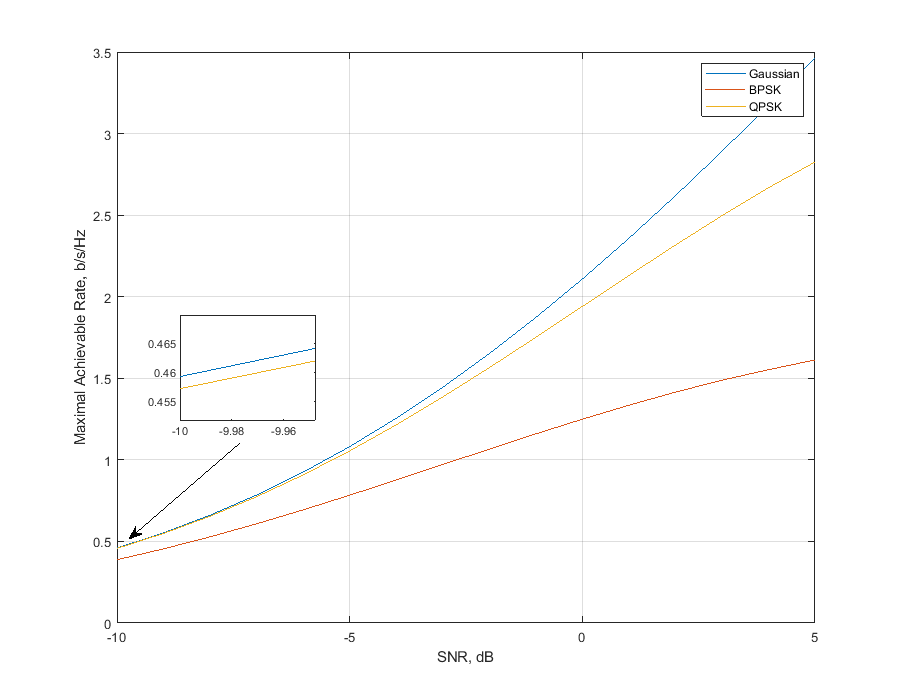
Figure 9: The maximal rate achieved by Gaussian inputs, QPSK, and BPSK in a RIS MIMO system over a Rayleigh fading channel and transmit antennas $t=2$ and receive antennas $r=1$, and $N_{ris}=4$

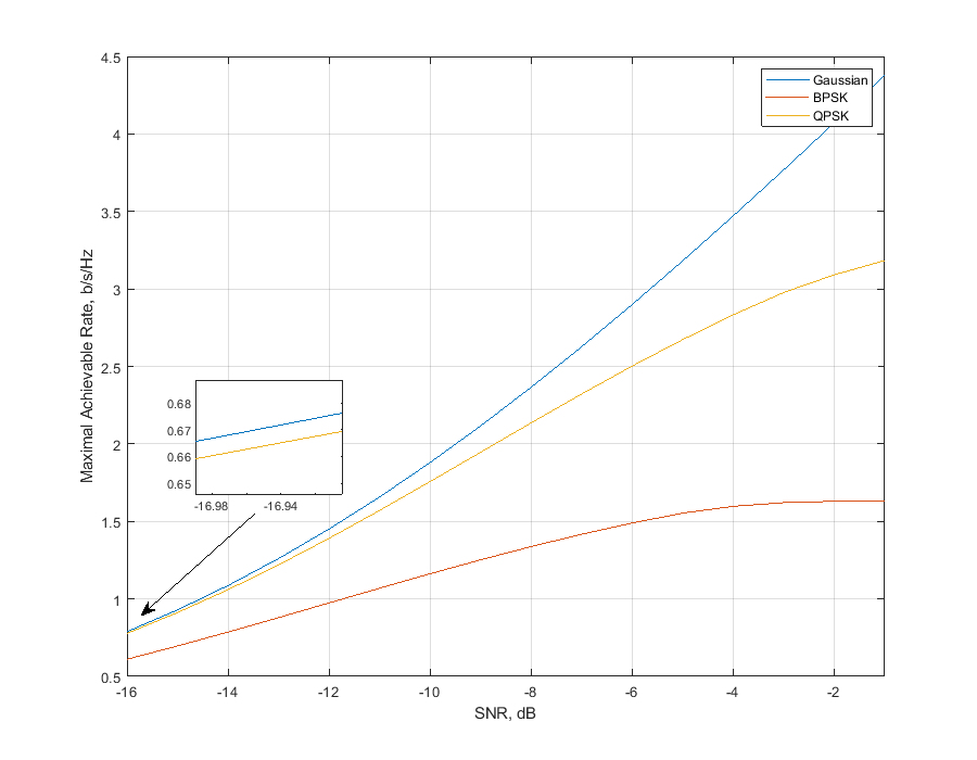
Figure 10: The maximal rate achieved by Gaussian inputs, QPSK, and BPSK in a RIS MIMO system over a Rayleigh fading channel and transmit antennas $t=2$ and receive antennas $r=1$, and $N_{ris}=32$

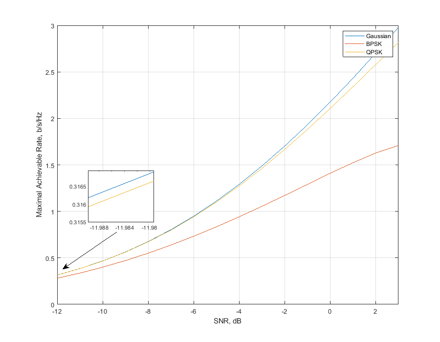
Figure 11: The maximal rate achieved by Gaussian inputs, QPSK, and BPSK in a RIS MIMO system over a Rayleigh fading channel and transmit antennas $t=3$ and receive antennas $r=1$, and $N_{ris}=4$

In Figs. 9 and 10, we illustrate the maximal achievable rates achieved by Gaussian inputs, QPSK and BPSK modulations in a RIS $2\times 1$ MIMO system with the number of the RIS elements $N_{ris}=4$ and $N_{ris}=32$, respectively. Fig. 9 shows that the capacity of the channel achieved by circularly symmetric complex Gaussian inputs increases without any boundary as the SNR increases. However, the trends of the maximal achievable rates of each modulation scheme are similar to the Gaussian inputs at the low SNR regime. Then, the gaps between the Gaussian input and the QPSK modulated input, the Gaussian input and the BPSK modulated input increase as the SNR increases. At the high SNR regime, according to [48], the upper bounds of the maximal rates achieved by BPSK and QPSK modulations go to $2$ bit/(channel use) for BPSK and $4$ bit/(channel use) for QPSK. In Fig. 10, the limits imposed by each modulation scheme are the same. However, the starting points move to smaller SNR values. When the number of the RIS elements increases, the channel condition becomes better and the required transmit power to achieve the same level of the rate decreases correspondingly. We change the number of the transmit antennas $t=3$ and $N_{ris}$ goes back to $4$. The result is shown in Fig. 11. At the same level of SNR$=2$dB, the maximal achievable rate of the QPSK modulation increases by $0.200$ bit/(channel use). The increasing trend in the $3\times 1$ MIMO case has not slowed down compared with the trend in Fig. 9. Moreover, the upper bounds of each modulation are $3$ bit/(channel use) for BPSK and $6$ bit/(channel use) for QPSK.

VI Conclusion

In this paper, we have established achievability and converse bounds on the maximal achievable rate $R(n,\epsilon)$ at a given blocklength $n$ and an average error probability $\epsilon$ for a RIS MIMO system. The analytical results demonstrated that the number of transmit and receive antennas and the channel variance $U(X;Y)$ would affect the convergence speed to the maximal achievable rate as the blocklength $n$ increases. In this work, we only considered memoryless modulation schemes, for our future work, we will extend our work to memory modulation schemes, such as [49, 50, 51, 52, 53, 54].

Appendix A Proof of Th. 4

In this Appendix, we show the complete proof of Th. 4. At first, we denote that the Mellin integral transform of $\exp{(-\frac{x}{\theta})}$ in (51) is

$$\mathcal{M}\{\exp{(-\frac{x}{\theta})}|s\}=\int_{0}^{\infty}x^{s-1}e^{(-\frac{x}{\theta})}dx=\theta^{s}\int_{0}^{\infty}x^{s-1}e^{-x}dx=\theta^{s}\Gamma(s),$$ (79)

and

$$\mathcal{M}\{x^{k}f(x)|s\}=\mathcal{M}\{f(x)|s+k\}.$$ (80)

Secondly, we derive that the Mellin transform of the PDF of the gamma variable in (51) as

$$\mathcal{M}\{f_{i}(x_{i})|s\}=\int_{0}^{\infty}x^{s-1}\frac{1}{\Gamma(k)\theta^{k}}x^{k-1}e^{-\frac{x}{\theta}}dx=\frac{\theta^{s-1}}{\Gamma(k)}\int_{0}^{\infty}x^{(k+s-1)-1}e^{-x}dx=\frac{\Gamma(k+s-1)}{\Gamma(k)}\theta^{s-1}.$$ (81)

Thus we can obtain the Mellin transform of $g(z)$, which is defined as the PDF of the product of $N$ independent random Gamma variables, as

$$\mathcal{M}\{g(z)|s\}=\prod_{i=1}^{N}\mathcal{M}\{f_{i}(x_{i})|s\}=\theta^{N(s-1)}\prod_{i=1}^{N}\frac{\Gamma(k+s-1)}{\Gamma(k)},$$ (82)

and

$$g(z) =\frac{1}{2\pi i}\int_{c-i^{\infty}}^{c+i^{\infty}}z^{-s}\theta^{N(s-1)}\prod_{i=1}^{N}\frac{\Gamma(k+s-1)}{\Gamma(k)}ds$$

$$=\frac{1}{2\pi i\theta^{N}}\int_{c-i^{\infty}}^{c+i^{\infty}}(\frac{z}{\theta^{N}})^{-s}\prod_{i=1}^{N}\frac{\Gamma(k+s-1)}{\Gamma(k)}ds$$

$$=(\frac{1}{\theta})^{N}\prod_{i=1}^{N}\frac{1}{\Gamma(k)}G^{\,N,0}_{0,N}\big{\lparen}\begin{smallmatrix}\\ k-1\end{smallmatrix}\big{|}\,\frac{z}{\theta^{N}}\big{\rparen}.$$ (83)

This completes the proof.

References

• [1] J. Leng, Z. Lin and P. Wang,”An implementation of an internet of things system for smart hospitals”,2020 IEEE/ACM Fifth International Conference on Internet-of-Things Design and Implementation (IoTDI), 254–255, 2020.
• [2] D. Zhai, H. Chen, Z. Lin. Y. Li and B. Vucetic, “Accumulate Then Transmit: Multi-user Scheduling in Full-Duplex Wireless-Powered IoT Systems”, IEEE Internet of Things Journal, Volume: 5 , Issue: 4 , Aug. 2018.
• [3] J. Wang, B. Li, G. Wang, Z. Lin, H. Wang, and G. Chen, Optimal Power Splitting for MIMO SWIPT Relaying Systems with Direct Link in IoT Networks, Physical Communication, Volume 43, December 2020.
• [4] Z. Lin, P. Xiao, T. B. Sørensen, and B. Vucetic, (2010), Spatial frequency scheduling for uplink SC-FDMA based linearly precoded multiuser MIMO systems. Eur. Trans. Telecomm., 21: 213-223. https://doi.org/10.1002/ett.1372
• [5] Z. Lin, P. Xiao and B. Vucetic, ”SINR distribution for LTE downlink multiuser MIMO systems,” 2009 IEEE International Conference on Acoustics, Speech and Signal Processing, 2009, pp. 2833-2836, doi: 10.1109/ICASSP.2009.4960213.
• [6] Z. Lin, T. B. Sorensen and P. E. Mogensen, ”Downlink SINR Distribution of Linearly Precoded Multiuser MIMO Systems,” in IEEE Communications Letters, vol. 11, no. 11, pp. 850-852, November 2007, doi: 10.1109/LCOMM.2007.071082.
• [7] S. Shaham, M. Ding, Z. Lin, R. Abbas, “Fast Channel Estimation and Beam Tracking for Millimeter Wave Vehicular Communications”, IEEE Access, vol. 7, pp. 141104-141118, 2019, doi: 10.1109/ACCESS.2019.2944308.
• [8] X. Wang, P. Wang, M. Ding, Z. Lin, F. Lin, B. Vucetic, and L. Hanzo, “Performance analysis of terahertz unmanned aerial vehicular net- works,” IEEE Transactions on Vehicular Technology, vol. 69, no. 12, pp. 16 330–16 335, 2020.
• [9] X. Wang, Z. Lin, F. Lin, and L. Hanzo, “Joint hybrid 3d beamforming relying on sensor-based training for reconfigurable intelligent surface aided terahertz-based multi-user massive mimo systems,” IEEE Sen- sors Journal, pp. 1–1, 2022.
• [10] Z. Chu, P. Xiao, D. Mi, W. Hao, Z. Lin, Q. Chen, and R. Tafazolli, “Wireless powered intelligent radio environment with non-linear energy harvesting,” IEEE Internet of Things Journal, pp. 1–1, 2022.
• [11] Y. Hu, P. Wang, Z. Lin, and M. Ding, “Performance analysis of reconfigurable intelligent surface assisted wireless system with low- density parity-check code,” IEEE Communications Letters, vol. 25, no. 9, pp. 2879–2883, 2021.
• [12] Y. Hu, P. Wang, Z. Lin, M. Ding, and Y.-C. Liang, ”Performance analysis of ambient backscatter systems with ldpc-coded source signals,” IEEE Transactions on Vehicular Technology, vol. 70, no. 8, pp. 7870–7884, 2021.
• [13] Y. Chen, M. Ding, D. L opez-Perez, X. Yao, Z. Lin, and G. Mao, ”On the theoretical analysis of network-wide massive mimo performance and pilot contamination,” IEEE Transactions on Wireless Communi- cations, vol. 21, no. 2, pp. 1077–1091, 2022.
• [14] Y. Hu, P. Wang, Z. Lin, M. Ding, and Y.-C. Liang, “Machine learning based signal detection for ambient backscatter communications,” in ICC 2019 - 2019 IEEE International Conference on Communications (ICC), 2019, pp. 1–6.
• [15] S. Xing, M. Ding, and Z. Lin, “Outage capacity analysis for ambient backscatter communication systems,” in 2018 28th International Telecommunication Networks and Applications Conference (ITNAC), 2018, pp. 1–6.
• [16] Z. Lin, B. Vucetic, J. Mao, ”Ergodic capacity of LTE downlink multiuser MIMO systems”, 2008 IEEE International Conference on Communications, 3345-3349.
• [17] G. Mao, Z. Lin, X. Ge, Y. Yang, ”Towards a simple relationship to estimate the capacity of static and mobile wireless networks”, IEEE transactions on wireless communications 12 (8), 2014, 3883-3895
• [18] J. Yue, Z. Lin and B. Vucetic, ”Distributed Fountain Codes With Adaptive Unequal Error Protection in Wireless Relay Networks,” in IEEE Transactions on Wireless Communications, vol. 13, no. 8, pp. 4220-4231, Aug. 2014, doi: 10.1109/TWC.2014.2314632.
• [19] M. Di Renzo et al., ”Reconfigurable Intelligent Surfaces vs. Relaying: Differences, Similarities, and Performance Comparison,” in IEEE Open Journal of the Communications Society, vol. 1, pp. 798-807, 2020.
• [20] J. Yue; Z. Lin; B. Vucetic; G. Mao; M. Xiao; B. Bai; K. Pang, ”Network Code Division Multiplexing for Wireless Relay Networks,” IEEE Transactions on Wireless Communications, vol.14, no.10, pp.5736-5749, Oct. 2015.
• [21] K. Pang, Z. Lin, Y. Li, B. Vucetic, ”Joint network-channel code design for real wireless relay networks”, the 6th International Symposium on Turbo Codes & Iterative Information, 2010, 429-433.
• [22] Z. Lin, A. Svensson, ”New rate-compatible repetition convolutional codes”, IEEE Transactions on Information Theory 46 (7), 2651-2659
• [23] Z. Lin, “Design of Network Coding Schemes in Wireless Network”, CRC Press — Taylor & Francis. Books, ISBN: 9781032067766, June 2022.
• [24] Z Lin, B Vucetic, ”Power and rate adaptation for wireless network coding with opportunistic scheduling”, 2008 IEEE International Symposium on Information Theory, 21-25
• [25] E. Basar, M. Di Renzo, J. De Rosny, M. Debbah, M. -S. Alouini and R. Zhang, ”Wireless Communications Through Reconfigurable Intelligent Surfaces,” in IEEE Access, vol. 7, pp. 116753-116773, 2019.
• [26] L. Yang, Y. Yang, M. O. Hasna and M. -S. Alouini, ”Coverage, Probability of SNR Gain, and DOR Analysis of RIS-Aided Communication Systems,” in IEEE Wireless Communications Letters, vol. 9, no. 8, pp. 1268-1272, Aug. 2020.
• [27] S. Zeng, H. Zhang, B. Di, Z. Han and L. Song, ”Reconfigurable Intelligent Surface (RIS) Assisted Wireless Coverage Extension: RIS Orientation and Location Optimization,” in IEEE Communications Letters, vol. 25, no. 1, pp. 269-273, Jan. 2021.
• [28] H. Guo, Y. -C. Liang, J. Chen and E. G. Larsson, ”Weighted Sum-Rate Maximization for Intelligent Reflecting Surface Enhanced Wireless Networks,” 2019 IEEE Global Communications Conference (GLOBECOM), 2019.
• [29] C. Huang, G. C. Alexandropoulos, A. Zappone, M. Debbah and C. Yuen, ”Energy Efficient Multi-User MISO Communication Using Low Resolution Large Intelligent Surfaces,” 2018 IEEE Globecom Workshops (GC Wkshps), 2018.
• [30] H. Han, J. Zhao, D. Niyato, M. D. Renzo and Q. -V. Pham, ”Intelligent Reflecting Surface Aided Network: Power Control for Physical-Layer Broadcasting,” ICC 2020 - 2020 IEEE International Conference on Communications (ICC), 2020.
• [31] A. A. Boulogeorgos and A. Alexiou, ”Performance Analysis of Reconfigurable Intelligent Surface-Assisted Wireless Systems and Comparison With Relaying,” in IEEE Access, vol. 8, pp. 94463-94483, 2020.
• [32] Y. Polyanskiy, H. V. Poor, and S. Verdú, “Channel coding rate in the finite blocklength regime,” IEEE Trans. Inf. Theory, vol. 56, no. 5, pp. 2307–2359, May 2010.
• [33] T. J. Cui, M. Q. Qi, X. Wan, J. Zhao, and Q. Cheng, “Coding metamaterials, digital metamaterials and programmable metamaterials,” Light, Sci. Appl., vol. 3, no. 10, p. e218, Oct. 2014.
• [34] H. Yang et al., “A programmable metasurface with dynamic polarization, scattering and focusing control,” Sci. Rep., vol. 6, no. 1, Oct. 2016, Art. no. 35692.
• [35] S. Zhang and R. Zhang, ”Capacity Characterization for Intelligent Reflecting Surface Aided MIMO Communication,” in IEEE J. Sel. Areas Commun., vol. 38, no. 8, pp. 1823-1838, Aug. 2020.
• [36] İ. E. Telatar, “Capacity of multi-antenna Gaussian channels,” Eur. Trans. Telecommun., vol. 10, pp. 585–595, Nov. 1999.
• [37] Y. Polyanskiy, “Channel coding: Non-asymptotic fundamental limits,” Ph.D. dissertation, Dept. Elect. Eng., Princeton Univ., Princeton, NJ, USA, 2010.
• [38] J. Neyman and E. S. Pearson, “On the problem of the most efficient tests of statistical hypotheses,” Philosoph. Trans. Roy. Soc. A, vol. 231, pp. 289–337, Jan. 1933.
• [39] H. V. Poor and S. Verdú, “A lower bound on the error probability in multihypothesis testing,” IEEE Trans. Inf. Theory, vol. 41, no. 6, pp. 1992–1993, 1995.
• [40] R. E. Blahut, “Hypothesis testing and information theory,” IEEE Trans. Inf. Theory, vol. 20, no. 4, pp. 405–417, 1974.
• [41] R. Ash, Information Theory. New York: Interscience Publishers, 1965.
• [42] Y. Polyanskiy, H. V. Poor, and S. Verdú, “Dispersion of Gaussian channels,” in Proc. 2009 IEEE Int. Symp. Inf. Theory (ISIT), Seoul, Korea, Jul. 2009.
• [43] S. Verdú, “Spectral efficiency in the wideband regime,” IEEE Trans. Inf. Theory, vol. 48, no. 6, pp. 1319–1343, Jun. 2002.
• [44] Springer, M. D., and W. E. Thompson. “The Distribution of Products of Beta, Gamma and Gaussian Random Variables.” SIAM J. Appl. Math., vol. 18, no. 4, 1970, pp. 721–737.
• [45] G. Wiechman and I. Sason, ”An Improved Sphere-Packing Bound for Finite-Length Codes Over Symmetric Memoryless Channels,” IEEE Trans. Inf. Theory, vol. 54, no. 5, pp. 1962-1990, May 2008.
• [46] I. Sason and S. Shamai, ”On improved bounds on the decoding error probability of block codes over interleaved fading channels, with applications to turbo-like codes.” IEEE Trans. Inf. Theory, vol. 47, no. 6, pp. 2275-2299, Sept. 2001.
• [47] W. Feller, An Introduction to Probability Theory and Its Applications, Second ed. New York: Wiley, 1971, vol. II.
• [48] Liu, Y.; Zhang, J.; Zhang, D. ”Saddle Point Approximation of Mutual Information for Finite-Alphabet Inputs over Doubly Correlated MIMO Rayleigh Fading Channels.” Appl. Sci., 2021, 11, 4700.
• [49] Z. Lin and T. Aulin, “Joint Source and Channel Coding using Punctured Ring Convolutional Coded CPM”, IEEE Transactions on Communications, Vol. 56, No. 5, May, 2007, pp. 712-723.
• [50] Z. Lin and T. Aulin, “On Combined Ring Convolutional Coded Quantization and CPM for Joint Source and Channel Coding”, Transactions on Emerging Telecommunications Technologies, Special Issue on ’New Directions in Information Theory’, Vol.19, No.4. June 2008, pp. 443-453.
• [51] Z. Lin and T. Aulin, “Joint Source-Channel Coding using Combined TCQ/CPM: Iterative Decoding”, IEEE Transactions on Communications, VOL.53, NO. 12, Dec. 2005, pp. 1991-1995.
• [52] Z. Lin and B. Vucetic, “Performance Analysis on Ring Convolutional Coded CPM”, IEEE Transactions on Wireless Communications, Vol. 8, No. 9, Sept. 2009, pp. 4848-4854.
• [53] Z. Lin and B. Vucetic, “Analytical Bounds on Symbol Error Probability of Ring Convolutional Coded CPM”, IEEE Communications Letters, Vol. 13, No. 6, June, 2009, pp. 372-374.
• [54] Z. Lin and T. Aulin, “On Joint Source and Channel Coding using trellis coded CPM: Analytical Bounds on the Channel Distortion”, IEEE Transactions on Information Theory, Vol. 53, No. 13, Sept. 2007. pp. 3081-3094.