Lie Algebraic Quantum Phase Reduction

Abstract

We introduce a general framework of phase reduction theory for quantum nonlinear oscillators. By employing the quantum trajectory theory, we define the limit-cycle trajectory and the phase space according to a stochastic Schrödinger equation. Because a perturbation is represented by unitary transformation in quantum dynamics, we calculate phase response curves with respect to Lie algebra. Our method shows that the proposed measurement induces synchronization and alters the phase response curves. The resulting clusters in the phase space form observable signature of the quantum synchronization, unlike indirect indicators obtained from density operators.

Introduction.— The last decade has witnessed a remarkable shift in the interest in synchronization, extending from classical dynamics to the quantum regime [1, 2, 3, 4]. Numerous studies have been reported on the synchronization of nonlinear oscillators that show quantum effects, such as spins [5, 6], optomechanical systems [7, 8], cold atoms [9, 10], quantum heat engines [11, 12, 13, 14], and (discrete or continuous) time crystals [15, 16, 17]. In fact, synchronization in quantum systems is critical for considerable advances in future quantum technologies, including quantum communication and cryptography [18, 19]. For example, recent studies have shown that quantum synchronization helps addressing important security issues in quantum key distribution protocols [20]. Therefore, exploring synchronization in the quantum regime holds great technological promise. In this direction, theoretical models of limit cycles (i.e., self-sustained oscillators adaptable to weak perturbations) have been proposed in open quantum systems, such as quantum van der Pol oscillators [21, 22, 23, 24, 25] and spin oscillators [26]. Furthermore, several experimental reports have demonstrated quantum synchronization of limit cycles in laboratory settings [6, 17, 27, 28]. Against this background, we propose a quantum phase reduction theory for continuous measurement to describe quantum limit cycles in phase dynamics. The phase reduction theory [29, 30] reduces the multidimensional dynamics of a weakly perturbed limit cycle to one-dimensional dynamics in the phase space. By continuously monitoring the environment to which oscillatory systems are coupled, quantum trajectories of the system come to obey a stochastic Schrödinger equation (SSE) [31, 32, 33]. When the effect of quantum noise is sufficiently weak, these trajectories fluctuate around a deterministic trajectory defined by the continuous measurement. However, since a perturbation in quantum limit-cycle dynamics differs from that in classical dynamics and is represented by a unitary transformation, we calculate the phase response to a perturbation based on Lie algebra. Thus, we can derive a quantum phase equation from a Lindblad master equation that describes a weakly perturbed dissipative system. Note that the proposed approach reproduces the conventional phase reduction theory in the classical limit. Furthermore, using quantum van der Pol oscillators, we show the proposal approach recovers the definitions of the limit-cycle trajectory, the phase, the perturbation, and the phase response curves of the conventional phase reduction theory. Whereas Ref. [34] reduces quantum dynamics to classical one in a semiclassical approximation and applies the conventional phase reduction theory to it, by employing Lie algebra, we develop the original framework of phase reduction theory directly applicable to quantum limit cycles in the Hilbert space. In the quantum regime, the trajectories of a system are obtained by continuous measurement, where the measurement itself affects the system’s dynamics. Accordingly, our proposed method reveals, through simulations of the quantum van der Pol oscillators, that the measurement induces synchronization and alters the phase response curve in the quantum regime. The resulting clusters visualize quantum synchronization and can be observed by continuous measurement, unlike the indirect indicators obtained from density operators.

Derivation.— In open quantum dynamics, quantum limit-cycle oscillators are usually described by a Lindblad equation [35, 36]. Let $\rho(t)$ be a density operator at time $t$ whose time evolution is governed by

$$\frac{d\rho}{dt}=-i[H,\rho]+\sum_{k=1}^{M}\mathcal{D}[L_{k}]\rho,$$ (1)

where $H$ is a Hamiltonian operator and $L_{k}$ are jump operators, and $\mathcal{D}[O]$ is the dissipater defined by $\mathcal{D}[O]\rho\equiv O\rho O^{\dagger}-(1/2)(O^{\dagger}O\rho+\rho O^{\dagger}O)$. To obtain a general phase reduction approach that can be applied to quantum limit cycle models, we do not specify the jump operators $L_{k}$. It is worth noting that a Lindblad equation describes a density operator, not the dynamics of the measurable quantum state. The latter are described using theory of quantum trajectory theory [37], which describes the stochastic evolution of a pure state of the system $\ket{\psi}$, obtained by continuously monitoring the environment. In the homodyne detection scheme, the evolution can be described by the following diffusive SSE in the Stratonovich form [31, 32, 33] (see [38] for details).

$$d\ket{\psi}= \left[-iH_{\mathrm{eff}}+\sum_{k=1}^{M}\frac{1}{2}\braket{L_{k}^{\dagger}L_{k}}+\braket{X_{k}}\left(L_{k}-\frac{\braket{X_{k}}}{2}\right)\right.$$

$$\left.+\frac{1}{4}\left(-2L_{k}^{2}+\braket{L_{k}^{2}}+\braket{L_{k}^{\dagger 2}}\right)\right]\ket{\psi}dt$$

$$+\sum_{k=1}^{M}\left(L_{k}-\frac{\braket{X_{k}}}{2}\right)\ket{\psi}\circ dW_{k}(t),$$ (2)

where $\circ$ denotes the Stratonovich calculus, $H_{\mathrm{eff}}\equiv H-(i/2)\sum_{k=1}^{M}L_{k}^{\dagger}L_{k}$ is a non-Hermitian operator (i.e., an effective Hamiltonian), and $X_{k}\equiv L_{k}+L_{k}^{\dagger}$ are quadratures of the system. Here, $\braket{O}$ denotes the expectation value of $O$ with respect to state $\ket{\psi}$, i.e., $\braket{O}\equiv\bra{\psi}O\ket{\psi}$. Random variables $dW_{k}$ are Wiener increments that satisfy $\mathbb{E}[dW_{k}]=0$, and $\mathbb{E}[dW_{k}^{2}]=dt$, where $\mathbb{E}[\cdot]$ denotes the average over all possible trajectories. The associated stochastic homodyne currents $J_{k}$ are defined as $J_{k}(t)\equiv\braket{X_{k}}+\xi_{k}(t)$, where $\xi_{k}(t)\equiv dW_{k}/dt$. In general, a limit-cycle trajectory in quantum dynamics and the phase space along it are not well defined. In the classical stochastic dynamics of limit cycles, a stochastic differential equation is represented by adding noise terms to a given deterministic differential equation [39, 40, 41, 42]. In contrast, quantum dynamics are stochastic in nature and the deterministic equation is not given. To realize a quantum phase reduction, the deterministic limit cycle and the phase along it should be defined. The classical deterministic limit-cycle dynamics corresponds to an equation obtained by removing noise terms from a stochastic differential equation in the Stratonovich form. As an analog of classical cases, we propose here to remove noise terms from an SSE in the Stratonovich form and define the resulting equation as the deterministic limit-cycle dynamics:

$$d\ket{\psi}= \left[-iH_{\mathrm{eff}}+\sum_{k=1}^{M}\frac{1}{2}\braket{L_{k}^{\dagger}L_{k}}+\braket{X_{k}}\left(L_{k}-\frac{\braket{X_{k}}}{2}\right)\right.$$

$$\left.+\frac{1}{4}\left(-2L_{k}^{2}+\braket{L_{k}^{2}}+\braket{L_{k}^{\dagger 2}}\right)\right]\ket{\psi}dt.$$ (3)

An SSE is usually represented and calculated in the Ito form for computational and statistical convenience. It is worth emphasizing that noise terms should be removed from an SSE in the Stratonovich interpretation, rather than in the Ito interpretation for the following reasons. The first is related to the chain rule of differentiation calculation. In fact, the phase reduction requires a coordinate transformation between a state vector and a phase coordinate. The transformation is performed via the chain rule of differentiation, which holds only in the Stratonovich form (not in the Ito form). The second reason is related to norm preservation. Note that the norm of Eq. (3) is preserved, $d\|\psi\|=0$, where $\|\psi\|\equiv\sqrt{\braket{\psi}{\psi}}$. Therefore, Eq. (3) stands on its own as pure-state dynamics, which is not the case for the Ito interpretation. It is a nontrivial property that an SSE with noise terms removed also stands as pure-state dynamics because, unlike the case for classical dynamics, the deterministic dynamics Eq. (3) is not given.

When Eq. (3) satisfies $\lim_{t\to\infty}|\braket{\psi(t)}{\psi(t+T)}|=1$ for a period $T$, $\ket{\psi}$ has a limit-cycle solution $\ket{\psi_{0}}$ to which $\ket{\psi}$ converges. Since $U(1)$ has no physical effect on the state $\ket{\psi}$ [43], the $U(1)$ transformation has no effect on the phase. We define the phase on a quantum limit cycle using the deterministic trajectory $\ket{\psi_{0}}$. There are several schemes for the phase reduction in classical stochastic systems [40, 41, 44]. For the sake of simplicity, we derive the phase equation by following the procedure in [40]. The phase $\theta$ is defined along the limit-cycle solution $\ket{\psi_{0}}$ using Eq. (3) as to change at a constant frequency $\omega=2\pi/T$. Furthermore, by virtue of the convergence to the limit-cycle solution $\ket{\psi_{0}}$, the phase $\theta$ outside of it is defined by an isochron under Eq. (3) as $\Theta\left(\ket{\psi(t)}\right)\equiv\Theta\left(\lim_{n\to\infty}\ket{\psi(t+nT)}\right)$, where the phase function $\Theta\left(\ket{\psi}\right)$ represents the phase at the state $\ket{\psi}$. Here, we assume that the perturbation is sufficiently weak, i.e., the state $\ket{\psi}$ is in the vicinity of the limit-cycle solution $\ket{\psi_{0}}$.

It should be mentioned that our definition of the phase response curve differs from that of the classical counterpart. While the state is defined in the Euclidean space for the classical limit cycle, the unitary group in the Hilbert space defines the state of a quantum limit cycle. Therefore, the corresponding bases are the generators of the unitary group $U(N)$ [45]. They can be decomposed into the generators of $U(1)$ and those of the special unitary group $SU(N)$. $U(1)$ represents the scalar multiplication, while $SU(N)$ is a unitary group with a determinant $\det[U]=1$. For example, the generators of $SU(2)$ correspond to Pauli matrices. By the definition of the phase, $U(1)$ has no effect on it. Thus, only $SU(N)$ should be considered in the phase space. In quantum limit cycles, the perturbation is represented by an infinitesimal unitary transformation and the phase response curve is calculated for it. Based on the Lie algebra, an arbitrary infinitesimal unitary transformation is represented by the Taylor expansion as $U\ket{\psi}=\exp\left(\sum_{l=1}^{N^{2}-1}-ig_{l}E_{l}-ig_{0}I\right)\ket{\psi}\simeq\ket{\psi}-\sum_{l=1}^{N^{2}-1}ig_{l}E_{l}\ket{\psi}-ig_{0}\ket{\psi}$, where $E_{l}$ are generators of $SU(N)$, $I$ is the identity matrix, and real coefficients $g_{l}$ satisfy $|g_{l}|\ll 1$. The phase response curves for the generators $E_{l}$ are represented as

$$Z_{l}(\theta)\equiv\lim_{g_{l}\rightarrow 0}\frac{\Theta(\exp(-ig_{l}E_{l})\ket{\psi_{0}(\theta)})-\Theta(\ket{\psi_{0}(\theta)})}{g_{l}},$$ (4)

where $\ket{\psi_{0}(\theta)}$ represents the state $\ket{\psi}$ on the limit-cycle solution $\ket{\psi_{0}}$ with phase $\theta$. Equation (4) describes the partial derivative with respect to a unitary transformation by generator $E_{l}$. This formulation defines the quantum phase response curve. For the case of high-dimensional systems, e.g., semiclassical systems, PRCs with respect to $N^{2}-1$ Lie algebra generators demand large computational resource. In such a case, we can calculate PRC either by a direct method with respect to an arbitrary Hamiltonian or an adjoint method in the Euclidean space (see [38] for details). Although Eq. (3) is not represented by Hermitian dynamics, an arbitrary infinitesimal change of a pure state can be represented by a unitary transformation. The stochastic terms in an SSE can be represented by traceless Hermitian operators as $d\ket{\psi}=-i\sum_{k=1}^{M}H_{k}\ket{\psi}\circ dW_{k}$ (see [38] for details), where traceless Hermitian operators $H_{k}$ are defined by

$$H_{k}\equiv i(L_{k}-\braket{L_{k}})\ket{\psi}\bra{\psi}+\mathrm{H.c.}$$ (5)

Due to the trace-orthogonal property of Lie algebra, traceless Hermitian operators $H_{k}$ can be decomposed into a linear combination of $SU(N)$ generators as $H_{k}=\sum_{l=1}^{N^{2}-1}g_{k,l}E_{l}$, where the coefficients $g_{k,l}$ are defined by $g_{k,l}\equiv\mathrm{Tr}[H_{k}E_{l}]$. Therefore, the following quantum phase equation is derived from the chain rule

$$\frac{d\theta}{dt}=\omega+\sum_{k=1}^{M}\sum_{l=1}^{N^{2}-1}Z_{l}(\theta)g_{k,l}(\theta)\circ\xi_{k}(t),$$ (6)

where $g_{k,l}(\theta)$ is evaluated at $\ket{\psi}=\ket{\psi_{0}(\theta)}$ on the limit cycle. The phase equation (6) in the Stratonovich form can be converted into an equivalent equation in the Ito form [46]

$$\frac{d\theta}{dt}=\omega+\frac{1}{2}\sum_{k=1}^{M}\frac{dY_{k}(\theta)}{d\theta}Y_{k}(\theta)+\sum_{k=1}^{M}Y_{k}(\theta)\xi_{k}(t),$$ (7)

where $Y_{k}(\theta)=\sum_{l=1}^{N^{2}-1}Z_{l}(\theta)g_{k,l}(\theta)$. In the following, we shall elaborate on the difference between our approach and that in Ref. [34], which is the extant phase reduction approach for quantum systems. In a semiclassical approximation, Ref. [34] reduces quantum dynamics to classical one based on a quasi-probability distribution [47, 32], and applies the conventional phase reduction theory to it. In contrast, based on Lie algebra, our approach proposes the original framework of phase reduction theory directly applicable to the pure state $\ket{\psi}$ of quantum limit cycles in the Hilbert space. To explain the difference in detail, we examine the quantum van der Pol oscillator defined by

$$\dfrac{d\rho}{dt}=-i[a^{\dagger}a,\rho]+\gamma_{1g}\mathcal{D}[a^{\dagger}]\rho+\gamma_{1d}\mathcal{D}[a]\rho+\gamma_{2d}\mathcal{D}[a^{2}]\rho,$$ (8)

where $a$ and $a^{\dagger}$ are annihilation and creation operators, respectively. The quantum van der Pol model describes the limit-cycle dynamics at a quantum scale. In quantum systems, the measurement outcomes are stochastic in nature. Thus, the position $x=(1/\sqrt{2})(a+a^{\dagger})$ and the momentum $p=-(i/\sqrt{2})(a-a^{\dagger})$ are evaluated through their expectation values as $\braket{x}_{\rho}$ and $\braket{p}_{\rho}$, respectively, where $\braket{O}_{\rho}\equiv\mathrm{Tr}[O\rho]$. In the classical limit $\braket{a^{\dagger}a}_{\rho}\gg 1$ (i.e., the system is at a macroscopic scale), Eq. (8) gives the equation of the momentum as $\braket{\ddot{x}}_{\rho}+\braket{\dot{x}}_{\rho}=(1/\epsilon)\left\{1-(\braket{x}_{\rho}^{2}+\braket{\dot{x}}_{\rho}^{2})/{A_{c}}^{2}\right\}+O(\epsilon^{2})$, where $\epsilon\equiv\gamma_{1g}-\gamma_{1d}$ corresponds to the difference between two rates of one-particle gain and loss, and $A_{c}\equiv\sqrt{\epsilon/\gamma_{2d}}$ [22]. This equation recovers the classical van der Pol oscillator model up to $O({\epsilon}^{2})$. For the semiclassical approximation, the previous work in [34] can be applied only to systems near the classical limit $\gamma_{1g}\gg\gamma_{2d}$. In contrast, our approach can be applied to an arbitrary regime, including the deep quantum regime $\gamma_{2d}\gg\gamma_{1g}$. Similarly, our approach differs from Ref. [48], which is a feedback control scheme to enhance synchronization by applying the semiclassical phase reduction to a homodyne detection scheme.

Thus far, we have been concerned with regimes ranging from the semiclassical to the quantum regime. Historically, the phase reduction theory was demonstrated in the context of classical deterministic dynamics. In the following, we show that our quantum phase reduction theory reduces to the conventional phase reduction theory in the classical limit. Using the phase transformation: $\ket{\psi}\rightarrow e^{i\phi(t)}\ket{\psi}$, where $\phi(t)$ is a solution of a stochastic differential equation (see [38] for details), the diffusive SSE [Eq. (2)] is rewritten as [31, 49]

$$d\ket{\psi} =dt\biggl{[}-iH+\sum_{k=1}^{M}\Bigl{(}-\frac{1}{2}(X_{k}L_{k}-\braket{X_{k}L_{k}})$$

$$+\braket{X_{k}}(L_{k}-\braket{L_{k}})\Bigr{)}\biggr{]}\ket{\psi}+\sum_{k=1}^{M}(L_{k}-\braket{L_{k}})\ket{\psi}\circ dW_{k}.$$ (9)

In the classical limit, the state $\ket{\psi}$ is considered coherent and satisfies $a\ket{\psi}=\alpha\ket{\psi}$, $a^{\dagger}\ket{\psi}=\alpha^{*}\ket{\psi}+\ket{x}$, and $|\alpha|\gg 1$, where $\ket{x}=a^{\dagger}\ket{\psi}-\alpha^{*}\ket{\psi}$. In Eq. (9), the stochastic terms are very weak compared to the deterministic terms. Hence, the dynamics can be considered as deterministic. As discussed above, in the classical limit, the quantum van der Pol oscillator model recovers the classical model in the Euclidean space. Similarly, by calculating the expectation value along the limit cycle in the Hilbert space, our definition of the limit cycle is equivalent to the conventional one in the classical limit. Moreover, this equivalence applies also to the perturbation and phase response. The perturbation in the Euclidean space is reproduced by the momentum operator $p$ in the Hilbert space as follows: By the unitary perturbation $d\ket{\psi}/dt=-ip\ket{\psi}$, the derivative of the expectation value of the position is unity, i.e., $d\braket{x}/dt=-i\braket{[x,p]}=1$. An arbitrary real perturbation, $d\braket{x}/dt=f(t)$, in the Euclidean space is then obtained by a unitary perturbation in the Hilbert space, $d\ket{\psi}/dt=-if(t)p\ket{\psi}$. It follows that the phase response can be calculated similarly for both the conventional and our proposed approach, which is connected with the conventional approach in the classical limit.

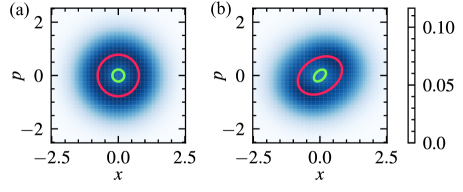
Figure 1: Wigner function and limit-cycle trajectories of quantum and semiclassical phase reduction approaches in the two-parameter settings quantum regime, (a) $(\Delta$, $\Omega$, $\eta\mathrm{e}^{i\lambda}$, $\gamma_{1g})/\gamma_{2d}=(1$, $0$, $0$, $0.1)$ and (b) $(\Delta$, $\Omega$, $\eta\mathrm{e}^{i\lambda}$, $\gamma_{1g})/\gamma_{2d}=(1$, $0$, $-0.2$, $0.1)$. Color intensity is proportional to the quasi-probability of the Wigner function. The limit-cycle trajectory of the quantum phase reduction (red line) passes through the high quasi-probability region of the Wigner function, while that of the semiclassical phase reduction (green line) does not. The fidelity $F(\rho_{1},\rho_{2})\equiv\mathrm{Tr}\left[\sqrt{\sqrt{\rho_{1}}\rho_{2}\sqrt{\rho_{1}}}\right]^{2}$ between the true density operator and those reconstructed from the phase distribution are (a) $0.958$, (b) $0.979$ in our method, and (a) $0.812$ in the semiclassical method.

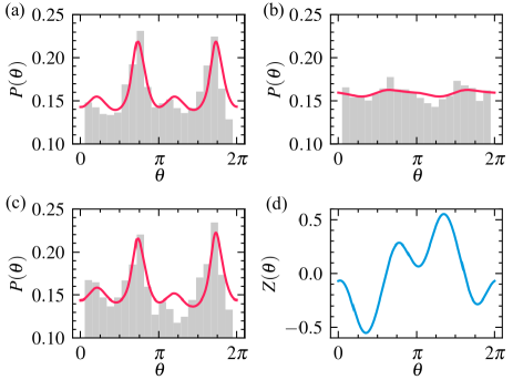
Figure 2: Phase distribution $P(\theta)$ in steady state and PRC $Z(\theta)$. (a), (b), and (c) Phase distribution (a) in quantum regime, (b) in deep quantum regime, and (c) subjected to harmonic drive as weak perturbation. (d) PRC with respect to harmonic drive Hamiltonian. The gray histograms are computed from SSE simulations and the red lines are computed from simulations of the proposed phase equation for (a), (b), and (c). The strength of the weak perturbation is $\Omega_{p}=0.05$ for (c). The parameters are $(\Delta$, $\Omega$, $\eta\mathrm{e}^{i\lambda}$, $\gamma_{1g})/\gamma_{2d}=(1$, $0$, $0$, $0.5)$ for (a), (c), and (d), $(\Delta$, $\Omega$, $\eta\mathrm{e}^{i\lambda}$, $\gamma_{1g})/\gamma_{2d}=(1$, $0$, $0$, $0.1)$ for (b).

Example.— As an example, we consider the quantum van der Pol oscillators in a rotating frame [22]:

$$\dfrac{d\rho}{dt}=-i[H,\rho]+\gamma_{1g}\mathcal{D}[a^{\dagger}]\rho+\gamma_{1d}\mathcal{D}[a]\rho+\gamma_{2d}\mathcal{D}[a^{2}]\rho,$$ (10)

where $H=-\Delta a^{\dagger}a+i\Omega(a^{\dagger}-a)+i\eta(a^{2}\exp(-i\lambda)-a^{\dagger 2}\exp(i\lambda))$ is the Hamiltonian, $\Delta=\omega_{d}-\omega_{0}$ is the detuning between the system’s natural frequency $\omega_{0}$ and a harmonic drive frequency $\omega_{d}$, $\Omega$ is the strength of the harmonic drive, and $\eta$ and $\lambda$ are the strength and phase of squeezing, respectively. In a rotating frame, the system rotates with a harmonic drive frequency $\omega_{d}$. First, we numerically validate the accuracy of the approximation by comparing the derived phase equation to the semiclassical phase equation. Figure 1 shows the Wigner function in the steady state and the limit-cycle trajectory of each phase reduction method in the quantum regime. We calculate the reconstructed density operator $\rho_{re}\equiv\int d\theta P(\theta)\ket{\psi_{0}(\theta)}\bra{\psi_{0}(\theta)}$, where $P(\theta)$ is a probability density function of the phase $\theta$, for each phase reduction method. Furthermore, we compare their fidelity level to those of the true density operator [34]. Our method provides a better approximation than the semiclassical method (see the caption of Fig. 1 for details), because it reduces a pure state to the phase without the semiclassical approximation. Note that we cannot calculate fidelity for the semiclassical method in Fig. 1(b) because diffusion matrices of a semiclassical Langevin equation are not positive-semidefinite in some points. Next, we investigate the effect of the measurement and the harmonic drive on quantum synchronization in the quantum regime. In contrast to classical dynamics, the measurement affects the system’s trajectory in the quantum regime. For brevity of expression, we here approximate the quantum van der Pol oscillator by limiting the bosonic Fock state to the lowest $N$ levels [24]. In Fig. 2, $N=6$ for (a), (c) and (d), and $N=4$ for (b). In the quantum regime, the proposed method yields a good approximation, as shown in Fig. 2(a). Although the synchronization is weakened for the deep quantum regime in Fig. 2(b), in both cases, the measurement induces synchronization in the two phase points in Fig. 2(a) and (b). Furthermore, as a weak perturbation Hamiltonian $H_{p}=i\Omega_{p}(a^{\dagger}-a)$, a harmonic drive is added to the Hamiltonian $H$ and enhances synchronization in Fig. 2(c), where $\Omega_{p}$ is the strength of the weak perturbation. In Fig. 2(d), the PRC for the harmonic drive clearly differs from that in the semiclassical regime, i.e., a sinusoidal wave. Some indicators have been signatures of quantum synchronization, such as mutual information [50], quantum discord [51, 52], and entanglement [53]. The clusters in the phase space form a signature of quantum synchronization and can be observed by continuous measurement, unlike the indirect indicators obtained from a density operator.

Conclusion.— In this Letter, we proposed a quantum phase reduction formulation of a Lindblad equation in a continuous measurement scheme. We showed that, in the case, the quantum limit cycle is identified as a pure-state trajectory, and the phase response to a unitary transformation, such as a weak perturbation, is defined based on Lie algebra. This present study can be used to unveil quantum limit cycles. For instance, it is possible to obtain a quantum limit cycle through optimization of the phase response curve, as done previously for classical systems [54].