A Compacted Structure for Cross-domain learning on Monocular Depth and Flow Estimation

Abstract

Accurate motion and depth recovery is important for many robot vision tasks including autonomous driving. Most previous studies have achieved cooperative multi-task interaction via either pre-defined loss functions or cross-domain prediction. This paper presents a multi-task scheme that achieves mutual assistance by means of our F2D, D2F, and EMA. F2D and D2F mechanisms enable multi-scale information integration between optical flow and depth domain based on differentiable shallow nets. A dual-head mechanism is used to predict optical flow for rigid and non-rigid motion based on a divide-and-conquer manner, which significantly improves the optical flow estimation performance. Furthermore, to make the prediction more robust and stable, EMA is used for our multi-task training. Experimental results on KITTI datasets show that our multi-task scheme outperforms other multi-task schemes and provide marked improvements on the prediction results.

I INTRODUCTION

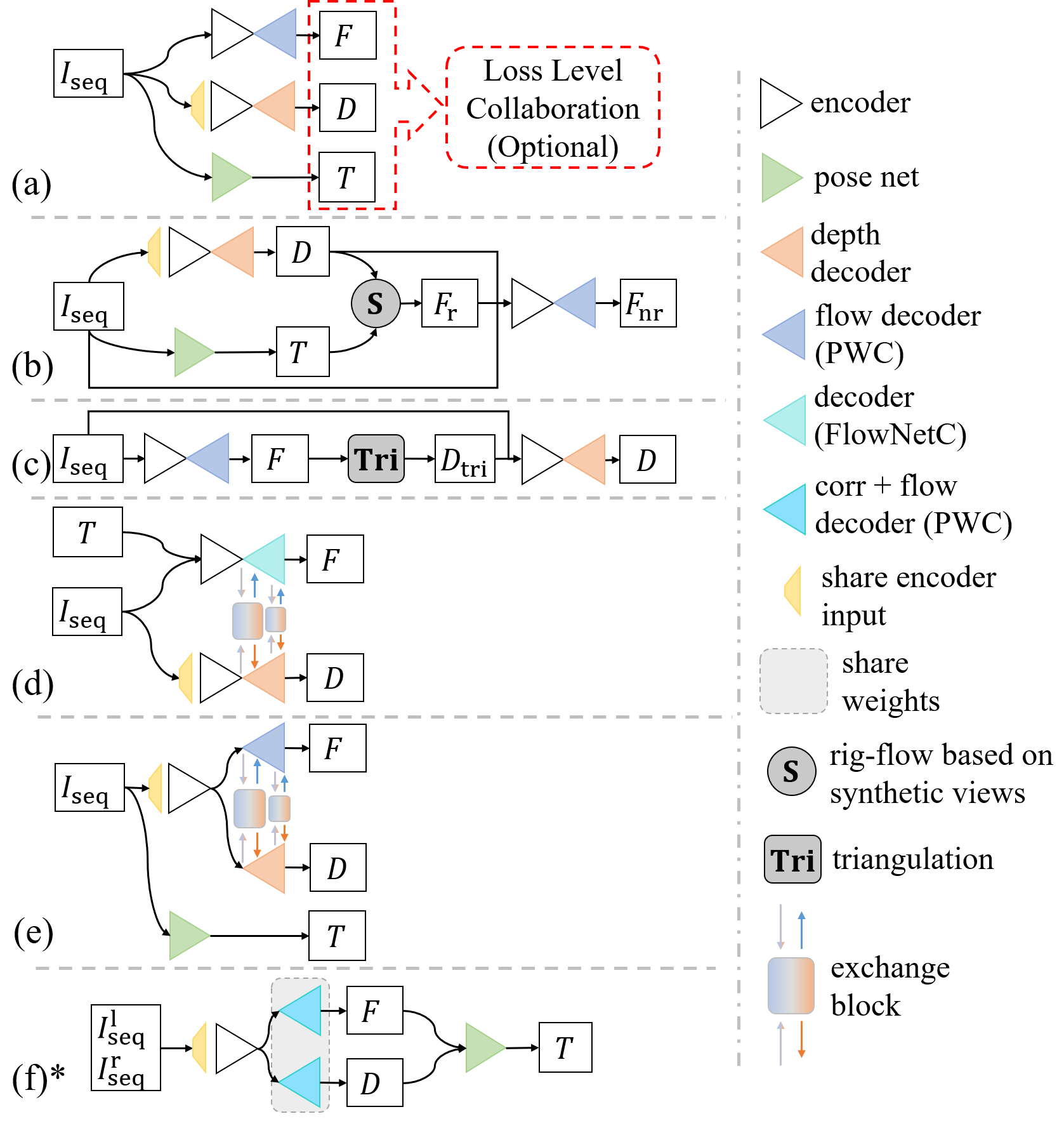
Figure 1: Unsupervised multi-task scheme. (a) Task specified separate network scheme supervised only by 3D geometry based loss functions (share encoder input: the encoder processes each images separately and the same below); (b) Flow estimation based on the rigid flow from synthetic views and original image sequence; (c) Triangulated depth based on estimated optical flow; (d) and (e) Information exchange block based coupled depth and optical flow network with/without known pose; (f) Joint stereo depth and optical flow estimation using shared weight decoder, combined with pose estimation based on the above results. (* refers to stereo depth different from monocular depth in other schemes)

3D scene understanding from single view video sequences is an important topic in robot vision, which consists of several classic computer vision tasks, including depth estimation, optical flow estimation, and visual odometry prediction. It plays a key role in many real-world applications, including autonomous driving [1], UAV [2], and surgical navigation [3, 4].

Depth Estimation. Traditional method referred to as SFM addresses depth and camera pose estimation simultaneously by keypoint matching. However, traditional methods tend to use hand-crafted features and often rely on sparse correspondence of low-level features [5, 6].

More recently, CNN have shown to be able to establish dense mapping relationships between single view images and the corresponding depth information in a supervised manner [7, 8, 9]. Nevertheless, the requirement of depth annotations is a major challenge for supervised methods [10, 11, 12]. Without any dependence on depth annotations, self-supervised methods [13, 14, 15] are trained with only stereo images by leveraging the multi-view geometric constraints and capable of monocular depth estimation. Zhou et al. [16] proposed a self-supervised monocular depth estimation paradigm by combining ego pose estimation and depth estimation tasks. By leveraging the appearance similarity indicators calculated by synthetic views [17] from temporal continuous frames and the current frame, these methods show promising performance w.r.t. other self-supervised methods. However, simple appearance loss is insufficient as supervision especially in illumination variations scenes. To this end, Xiong et al. [18] proposed several novel scale-consistent geometric constraints by jointly considering relative forward-backward poses consistency and depth reconstruction error to further improve the depth estimation performance.

Optical Flow Estimation. Optical flow estimation was traditionally be treated as an optimization problem over the dense displacement fields between temporal adjacent image pairs [19, 20]. The optimization objective consists of two main terms: 1) data – that encourages correlations in visually similar regions; 2) regularization – that penalizes incoherent motion fields according to the motion priors. Whilst offering good performance in general, the inherent optimization process entails high computational cost making these methods difficult to be used for real-time applications [21].

Recently, CNN-based approaches have shown improved optical flow estimation results [22, 21, 23]. However, these supervised methods require dense per-pixel optical flow annotation, which is laborious. By optimizing photometric consistency and local flow smoothness, unsupervised methods overcome the need for annotations. Several recent methods have greatly improved prediction results by checking forward-backward consistency [24], filtering range map to omit occlusion regions [25] or using loss function based on occlusion-aware bidirectional flow estimation and the robust census transform [26]. Unlike coarse-to-fine optical flow prediction, such as PWC-Net [21], more accurate results have been obtained by methods applying RNN structures to optical flow prediction scenarios [23].

Unsupervised Multi-task Network Scheme. Depth and optical flow can be estimated in a joint manner due to their inherent geometric correspondences. Many approaches [27, 28, 29] have predicted depth and optical flow with separate networks trained by geometric constraints based consistency losses. Other methods [30, 31, 32, 33] have combined depth and optical flow networks by serving depth or optical flow estimation results as the 3D information supervision of the other task. Although efficient, the above methods omit the inherent correspondence between latent information of different domains, which also serve as important assistance to multi-task estimation.

To further improve the multi-task network performance, we propose a novel multi-task scheme for depth estimation and optical flow prediction. It enables a bidirectional interaction of latent information between the depth and optical flow networks, enabling mutual assistance between two tasks. Our contributions can be summarised as follows:

• We proposed D2F and F2D mechanisms, which allow the latent information of depth and optical flow prediction transfer to and assist the estimation of the other task.

• For the former mechanism, we adopt the EMA to the multi-task learning and further improve the performance of cross-task collaboration.

• Dual-head mechanism is designed to enhance the optical flow prediction results by implicitly disentangling the representation of foreground and background.

To prove the effectiveness of our multi-task scheme, experiments are conducted on KITTI [34] datasets. The experiments cover different combinations of D2F, F2D, EMA training approach, and dual-head mechanism based on the baseline scheme in Fig. 1(a). F2D and D2F enable the interchange of latent information between depth and optical flow estimation. Experiment results show that our D2F mechanism can significantly improve the optical flow prediction accuracy. At the same time, the road signs and streetlamps are more clearly told in depth estimation. Experiments also show that our F2D can further improve depth estimation accuracy. We further show that our EMA training approach can improve both depth and optical flow prediction results. Our dual-head mechanism enables the division of the motion field into rigid and non-rigid parts based on a divide-and-conquer manner and improves the optical flow accuracy significantly.

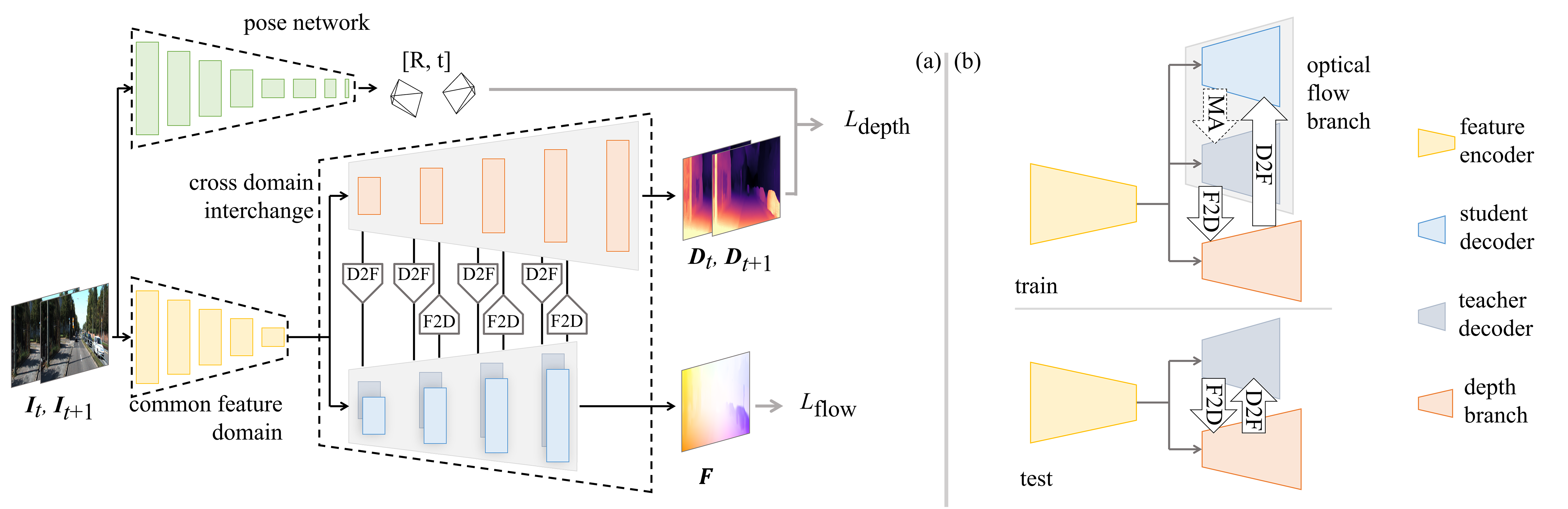
Figure 2: The overall architecture of the proposed network.

II RELATED WORK

II-A Loss-level Collaboration in Parallel Multi-task Network

Previous methods achieve cross-task interaction by applying cross-domain loss functions to multi-task learning scheme combined with separate single-task networks, as illustrated in Fig. 1(a). Ranjan et al. [30] introduced a competitive collaboration strategy that can classify moving objects and static background and effectively coordinate the training of the multi-task network. Benefiting from the framework, these tasks with inherent correspondence could reinforce each other. To reduce the violation of non-rigid motion flow caused by moving objects and occluded pixels, Wang et al. [31] constructed various masks for a valid consistency loss calculation, which remarkably improves the estimation of monocular depth, ego pose, and optical flow in temporal consecutive frames. Cao et al. [32] proposed photometric loss accompanied with bundle adjustment modules to achieve more accurate results. Zhao et al. [33] facilitated pose estimation by directly calculating camera pose from optical flow to improve depth estimation and optical flow prediction.

II-B Cross-task Boosting in Multi-task Network

Other than cross-task collaboration based on the loss functions, other methods took further steps to boost multi-task performance by introducing information interaction between the depth and optical flow estimation network. GeoNet et al. [35, 36] derives rigid flow from depth and pose prediction, which is then fine-tuned by optical flow network as illustrated in Fig. 1(b). By grafting the depth estimation network behind the flow-motion network, the method proposed by [37] refines the camera poses from GPS, IMU, or odometry algorithms and depth estimation with the confidential map as illustrated in Fig. 1(c). Yang et al. [38] have been estimated depth map based on optical flow from pretrained FlowNet with mid-point triangulation method. DRAFT [39] generates coarse depth prediction by triangulation from optical flow estimated by RAFT [40]. DRAFT then estimates the fine-grained depth and scene flow by joint leveraging coarse depth prediction and pyramid correlation. Different from the methods mentioned above, our cross-task exchange mechanism D2F and F2D enables multi-scale latent information interchange and facilitates multi-level cross-domain collaboration between depth and optical flow estimation.

As for multi-task feature-level collaboration, Chi et al. [41] introduced a feature-level collaboration mechanism for the stereo depth estimation, flow prediction, and pose detection networks as illustrated in Fig. 1(f). Whereas our scheme is dedicated to more challenging monocular depth estimation tasks, rather than stereo depth estimation. Hur et al. [42] proposed an architecture to estimate depth and 3D motion simultaneously from a single decoder. In addition to the previous cross-task boosting scheme, DENAO [43] proposed multi-scale exchange blocks which deeply coupled depth and optical flow branches according to epipolar geometry constraints, as illustrated in Fig. 1(d). The auxiliary optical flow improves the depth predictions and in turn yields large improvements in optical flow accuracy. However, by leveraging known ego camera pose and the proposed epipolar layer, DENAO is a partially supervised multi-task scheme. We proposed a fully unsupervised multi-task scheme with cross-task information exchange blocks. The geometry constraints between optical flow and depth predictions are leveraged implicitly, rather than the explicit 3D-to-2D projection and SVD decomposition-based triangulation in DENAO.

III Methodology

Given a pair of consecutive frames $(\bm{I}_{t},\bm{I}_{t+1})$ from an unlabeled monocular video, our method estimates optical flow $\bm{F}$ between the two frames $(\bm{I}_{t},\bm{I}_{t+1})$ and the corresponding depth maps $\bm{D}_{t}$ and $\bm{D}_{t+1}$.

The overall architecture of the proposed method is illustrated in Fig. 2(a). The multi-task estimation network consists of a shared encoder extracting the common feature domain, a two-branch decoder regress in the depth and optical domain, and exchange blocks for cross-domain message interchanging. As described in Sec. III-A, the two branches in the cross domain interchange, respectively for estimation of depth and optical flow, collaborate in their tasks by transferring cross-domain latent information from multiple layers to each other.

EMA is embedded into our training framework to improve the depth and optical flow estimation as shown in Fig. 2(b), with the detail described in Sec. III-B. Following mean teacher method [44], the optical flow branch is further divided into student and teacher decoder. The structure of the two optical flow decoders is adopted from PWC-Net [21] with dual-head mechanism (Sec. III-C) incorporated in each decoder layer. The depth branch contains a depth decoder following the decoder structure of monodepth [45].

A separate camera pose prediction network is applied during training for jointly learning depth and camera pose based on geometric consistency.

III-A Cross-domain Collaboration

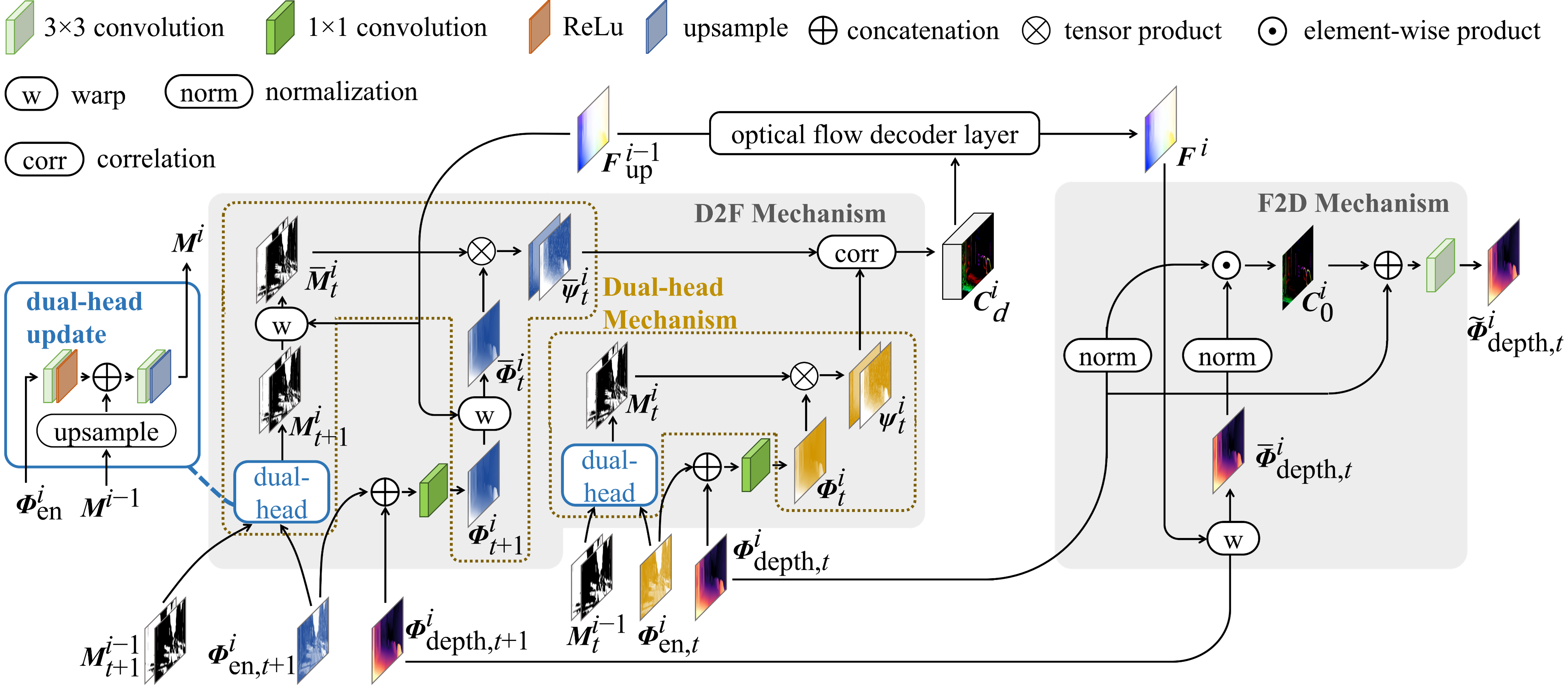
Figure 3: The architecture of $i^{\rm th}$ D2F, F2D, and Dual-head module. The D2F module calculates cost volume $\bm{C}$ from depth feature map $\bm{\Phi}_{\mathrm{depth}}^{i}$, encoder feature map $\bm{\Phi}_{\mathrm{en}}^{i}$, and dual-head mask $\bm{M}^{i-1}$. The F2D mechanism refine depth feature map $\bm{\Phi}_{\mathrm{depth}}^{i}$ into $\tilde{\bm{\Phi}}_{\mathrm{depth}}^{i}$. The Dual-head module transfer fused feature map $\bm{\Phi}^{i}$ into dual-head feature map $\bm{\Psi}^{i}$.

Estimation of depth and optical flow both requires comprehensive understanding of stereo vision. We hypothesize that these two tasks can be solved from a common feature domain and thus utilize only one shared encoder. For further mutually benefiting the two tasks in the exchange blocks, depth and optical flow branches collaborate with each other via D2F and F2D mechanisms. D2F and F2D mechanisms help to refine the prediction from multiple levels of the decoder layers by providing each other with cross-domain information, rather than merely supervising the final prediction of the entire network.

III-A1 D2F mechanism

In solitary optical flow prediction, the network determines the pixel shift by comparing the RGB information of two images. Benefiting from D2F mechanism, the depth branch provides additional geometric information for optical flow prediction.

D2F mechanism provides depth information of the images for optical flow prediction. As shown in Fig. 3, the $i^{\rm th}$ D2F mechanism takes dual-head masks $\bm{M}^{i-1}$ received from the $(i-1)^{\rm th}$ decoder layer, encoder feature maps $\bm{\Phi}_{en}^{i}$, and depth feature maps $\bm{\Phi}_{depth}^{i}$ from two frames of images as input to generate cost volume $\bm{C}_{d}^{i}$. Together with the cost volume, the up-sampled optical flow from the $(i-1)^{\rm th}$ decoder layer $\bm{F}^{i-1}$ is further refined by the $i^{\rm th}$ optical flow decoder layer to generate $\bm{F}^{i}$.

As the pre-process, the D2F mechanism first generates fused feature map, $\bm{\Phi}^{i}$ by $\bm{\Phi}^{i}=\mathrm{\mathcal{C}^{1}}\left(\bm{\Phi}_{\rm en}^{i}\oplus\bm{\Phi}_{\rm depth}^{i}\right)$ where $\oplus$ denotes the channel concatenation and $\mathrm{\mathcal{C}^{1}}$ denotes 1$\times$1 convolutional layers. $\bm{\Phi}^{i}$ will be then operated by dual-head mechanism to produce refined feature map $\bm{\Psi}^{i}$, which is discussed in section III-C.

The cost volume $\bm{C}_{d}^{i}$ is obtained through the correlation between $\bm{\Psi}_{t}^{i}$ and $\overline{\bm{\Psi}}_{t}^{i}$ with a limited range of $d$ pixels:

$$\bm{C}_{d}^{i}\left(\bm{\Psi}_{t}^{i},\overline{\bm{\Psi}}_{t}^{i}\right)=\frac{1}{N}\left(\bm{\Psi}_{t}^{i}+\bm{o}\right)^{\top}\left(\overline{\bm{\Psi}}_{t}^{i}+\bm{o}\right),\bm{o}\in[-d,d]\times[-d,d]$$ (1)

where N denotes the length of the column vector $\bm{\Psi}_{t}^{i}$.

III-A2 F2D Mechanism

The F2D mechanism improves depth prediction with the stereo features extracted from optical flow.

As illustrated in Fig. 3, the F2D mechanism obtain $\bm{F}^{i}$ to help improve the depth feature map $\bm{\Phi}_{\rm depth}^{i}$ and produce the refined depth feature map $\tilde{\bm{\Phi}}_{\rm depth}^{i}$.

We first normalize the value of $\overline{\bm{\Phi}}^{i}$ to [0,1]. The normalized feature maps are then applied to calculate the cost map $\bm{C}_{0}$ following Equation (1) where $d$ is set to 0.

The output refined depth feature map $\tilde{\bm{\Phi}}_{t}^{i}$ is calculated with $\tilde{\bm{\Phi}}_{t}^{i}=\mathrm{\mathcal{C}^{3}}\left(\bm{\Phi}_{t}^{i}\oplus\bm{C}_{0}\right)$ where $\mathrm{\mathcal{C}^{3}}$ denotes the 3$\times$3 convolutional layer. The refined depth feature map will be obtained by the next depth decoder layer.

III-B EMA for Cross-task Prediction

In our model, cross-domain information walks double-sided between depth and optical flow branches. Parameter fluctuation of any of these two branches will directly affect the other one. Moreover, D2F and F2D work at multiple decoder layers. The error of one layer will accumulate at the next layer, and will eventually cause significant bias on the final prediction result. These factors might cause the network not to converge easily to the optimal solution during training.

To make the prediction more robust and stable, we train and test the optical flow branch following EMA approach. EMA [44] was adapted to the CNN training to facilitate the semi-supervised classification result by averaging model weights instead of predictions. During training, the teacher model updates its parameters by using the EMA weights of the student model. To the best of our knowledge, this is the first application of EMA to cross-task prediction of depth and optical flow.

As illustrated in Fig. 2(b), the optical flow branch contains teacher and student decoders. Both decoders share the same architecture and initial parameters as well. The teacher decoder only works during training. During training, the student branch updates its parameters with back-propagation. For each training step, the teacher branch is updated in moving average approach according to the parameters of student branch. Only the feature maps predicted by the teacher decoder are given as the input of the F2D mechanism while the depth branch affiliates optical flow prediction by feeding student decoder feature maps via D2F mechanism. After being trained, the model discards the student decoder and the F2D mechanism extracts optical flow maps from teacher decoder.

III-C Dual-head Mechanism

Self-attention based framework [46, 47] avoids the locality in recurrent operations by making full use of global dependencies between input and output. The self-attention framework with multi-head attention mechanism can capture information from different representation subspaces and further achieve better performance. Zheng et al. [48] proposed a RA module to decouple different motions of nearby objects with a multi-head mask. While in this paper, inspired by the use of multi-head attention and following the idea of divide-and-conquer, we adopted dual-head disentanglement for D2F mechanism to further improve the optical flow estimation performance by decoupling the rigid and non-rigid motions.

The dual-head mechanism is applied to divide optical flow into rigid and non-rigid motion field representation. As shown in Fig. 3, each dual-head mask $\bm{M}^{i}$ is updated from the combination of the encoder feature map $\bm{\Phi}_{en}^{i}$ and the upsampled previous dual-head mask $\bm{M}^{i-1}$. While the first mask $\bm{M}^{1}$ is updated from the encoder feature map $\bm{\Phi}_{en}^{1}$ only:

$$\bm{M}^{i}=\left\{\begin{array}[]{cl}\varsigma\left(\mathrm{\mathcal{C}^{3}}\left(\mathrm{ReLU}\left(\mathrm{\mathcal{C}^{3}}\left(\bm{\Phi}_{\rm en}^{i}\right)\right)\oplus\mathrm{up}\left(\bm{M}^{i}\right)\right)\right),&i=2,3,4\\ \varsigma\left(\mathrm{\mathcal{C}^{3}}\left(\mathrm{ReLU}\left(\mathrm{\mathcal{C}^{3}}\left(\bm{\Phi}_{\rm en}^{i}\right)\right)\right)\right),&i=1\end{array}\right.$$ (2)

where $\rm\varsigma(\cdot)$ and $\rm ReLU(\cdot)$ respectively denotes sigmoid and ReLU operation.

The dual-head feature map $\bm{\Psi}_{t}^{i}$ of image $\bm{I}_{t}$ is generated by the tensor product of $\bm{M}_{t}^{i}$ and $\bm{\Phi}_{t}^{i}$. Meanwhile, $\bm{M}_{t+1}^{i}$ and $\bm{\Phi}_{t+1}^{i}$ are first warped by $\bm{F}_{\rm up}^{i-1}$ into $\overline{\bm{M}}_{t}^{i}$ and $\overline{\bm{\Psi}}_{t}^{i}$ before conducting tensor product operation.

III-D Experiments Implementation

In this section, we validate the improvement of (1) the cross-task collaboration, (2) the dual-head mechanism, and (3) the EMA approach to depth evaluation and optical flow prediction. The network is trained on KITTI’s data spit of Eigen et al. [49] following Zhou et al.’s [16] pre-processing. We train the network in the following steps:

(1) The feature encoder and the depth branch are trained with the learning rate of $10^{-4}$ for 20 epochs.

(2) The optical flow decoder branch and D2F blocks are further connected into the network. The network is trained with the learning rate of $10^{-4}$ for another 20 epochs.

(3) Finally, we add the F2D block for depth evaluation assistance. The network is trained with the learning rate of $10^{-5}$ for 5 epochs.

We trained our network using depth loss $L_{\rm depth}$ and optical flow loss $L_{\rm flow}$ following [50] and [21], respectively. Adam optimizer [51] is used in all of the training steps. The size of the images is $1024\times 320$. We validate the depth estimation result on the Eigen et al.’s testing split, and the optical flow prediction result on KITTI 2015 training set.

IV RESULTS

IV-A Ablation Study

Model	Components	Parameters	FPS	Depth							Optical Flow
				abs rel$\downarrow$	sq rel$\downarrow$	rms$\downarrow$	log rms$\downarrow$	$\rm\delta_{1}\uparrow$	$\rm\delta_{2}\uparrow$	$\rm\delta_{3}\uparrow$	epe$\downarrow$	epe noc$\downarrow$	F1(%)$\downarrow$
I	Baseline	19.97M	-	0.115	0.885	4.705	0.190	0.879	0.961	0.982	8.20	4.53	24.35
II	I + D2F	18.22M	12.8	0.117	0.954	4.878	0.195	0.878	0.960	0.980	6.73	3.23	20.65
III	II + F2D	19.00M	11.9	0.113	0.886	4.795	0.193	0.880	0.960	0.981	7.23	3.42	21.16
IV	III + EMA	19.00M	11.9	0.112	0.893	4.788	0.192	0.882	0.960	0.981	7.11	3.30	21.16
V	II + D-H	18.78M	8.1	0.117	1.000	4.859	0.194	0.880	0.960	0.980	6.23	2.88	19.88
VI	IV + D-H	19.55M	7.7	0.112	0.859	4.798	0.193	0.879	0.960	0.981	6.84	3.04	20.89

TABLE I: Ablation study indicating how the mechanisms we proposed affect the parameter amount, FPS, and prediction result of depth and optical flow. Baseline: monodepth2 [50] and PWC-Net [21] working separately. The parameter mount is the sum of these two networks. D2F: depth-to-flow mechanism. F2D: flow-to-depth mechanism. EMA: EMA approach. D-H: dual-head mechanism.

To validate the effect of each component of depth and optical flow prediction network, we tried different combinations of D2F mechanism, F2D mechanism, EMA approach, and dual-head mechanism in experiments. Tab. I shows the prediction results of the experiments with the various combinations, marked as I to VI. Fig. 4 and 5 illustrate the effect of D2F and dual-head mechanism to the result of optical flow and depth estimation. Fig. 6 further illustrates the trade-off between depth and optical flow prediction and adding different components to the network architecture.

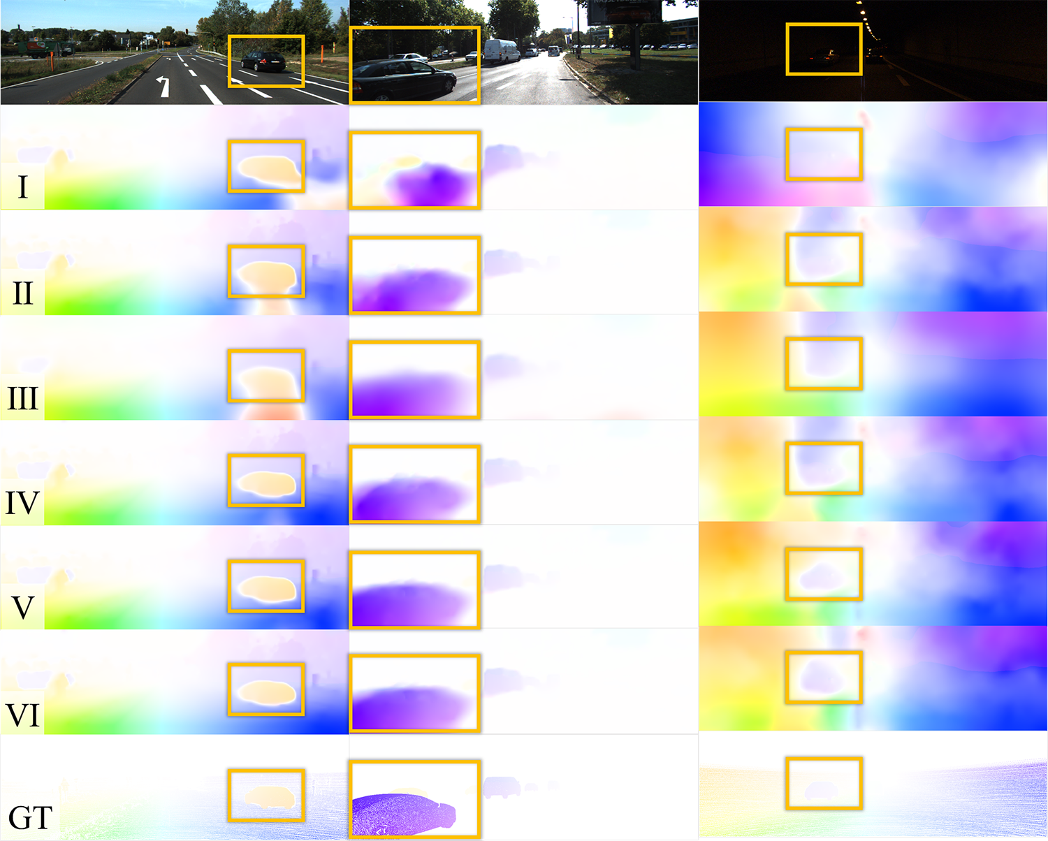
Figure 4: Illustration of the ablation study of optical flow prediction. From top to bottom: input color image and the prediction result of model I to VI, and the optical flow GT. In the orange boxes are vehicles or their respective optical flow.

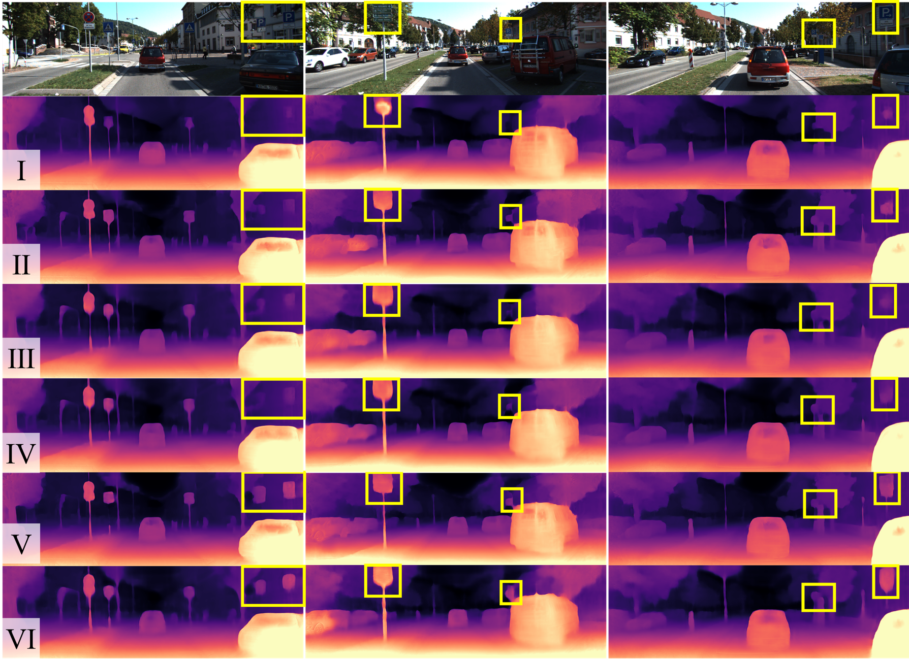
Figure 5: Illustration of the depth estimation. From top to bottom: input color image and the prediction result of model I to VI. In the yellow boxes, we show some road signs that are easy to be confused with the background buildings.

D2F mechanism can significantly improve the accuracy of optical flow prediction, which can be proved by comparing experiment I and II in Tab. I and Fig. 4. Furthermore, it can be seen from Fig. 5 that D2F mechanism can also support the depth branch telling the road signs from the buildings. This might be because objects like road signs are closer to the camera and can generate optical flow different from the distant buildings, which can be detected by the optical flow branch.

The information generated from optical flow prediction facilitates depth estimation via F2D mechanism. This could be seen from the comparison of experiment I, II, and III in Tab. I. Experiment III and IV also demonstrates that EMA approach can benefit both depth and optical flow prediction.

Experiment V and VI, respectively compared to experiment II and IV, prove that dual-head mechanism supports the optical flow prediction accuracy. The supporting role of dual-head mechanism can also be seen in Fig.  4 and 5. As shown in Fig. 4, comparing to baseline, with or without D2F mechanism’s assistance, adding dual-head mechanism to the architecture can significantly improve the network’s ability to recognize moving objects like vehicles – even in the dark tunnel. Fig. 5 shows that during depth estimation, the network with dual-head mechanism can also help distinguish between buildings and road signs.

Fig. 6 tells how the different components affect the two tasks of the network. D2F mechanism significantly improves optical flow prediction while causing the depth estimation accuracy slightly drops. A similar effect was achieved with F2D, enhances the accuracy of depth prediction while mildly reducing the effect of optical flow prediction. EMA approach achieves a positive effect on both tasks and dual-head mechanism facilitates optical flow prediction with little impact on depth estimation.

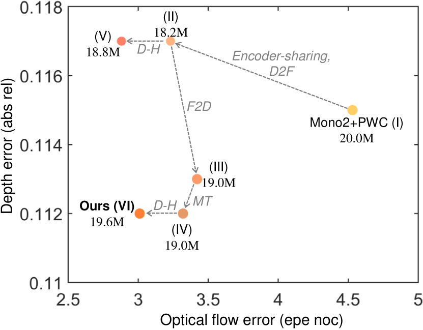
Figure 6: Bubble chart indicating the trade-off of depth and optical flow prediction accuracy, represented with absolute relative error and non-occluded pixels endpoint error, of model I to VI. The parameter mounts of models are shown with the size of the bubbles.

IV-B Depth and Optical Flow Evaluation

Method	Parameters	FPS	Scheme	abs rel$\downarrow$	sq rel$\downarrow$	rms$\downarrow$	log rms$\downarrow$	$\rm\delta_{1}\uparrow$	$\rm\delta_{2}\uparrow$	$\rm\delta_{3}\uparrow$	epe$\downarrow$	epe noc$\downarrow$	F1(%)$\downarrow$
zhou et al. [16]	-	-	-	0.183	1.595	6.709	0.270	0.734	0.902	0.959	-	-	-
monodepth2 [50]	-	-	-	0.115	0.882	4.701	0.190	0.879	0.961	0.982	-	-	-
Back2Future	-	-	-	-	-	-	-	-	-	-	7.04	-	24.21
Unflow [26]	-	-	-	-	-	-	-	-	-	-	8.10	-	23.27
DF-Net [27]	151.15M	-	(a)	0.150	1.124	5.507	0.223	0.806	0.933	0.973	8.98	-	26.01
GL-Net [28]	-	-	(a)	0.135	1.070	5.230	0.210	0.841	0.948	0.980	8.35	4.86	-
CC [30]	59.77M	7.8	(a)	0.140	1.070	5.326	0.217	0.826	0.941	0.975	6.27	4.17	29.15
DOP [31]	59.77M	7.9	(a)	0.140	1.068	5.255	0.217	0.827	0.943	0.977	6.66	-	23.04
GeoNet [35]	118.52M	0.2	(b)	0.147	0.936	4.348	0.218	0.810	0.941	0.977	10.81	8.05	-
Yang. [36]	-	-	(d)	0.139	1.297	5.879	0.223	0.827	0.936	0.979	9.87	6.45	-
Ours (V)	18.78M	8.1	(e)	0.117	1.000	4.859	0.194	0.880	0.960	0.980	6.23	2.88	19.88
Ours (VI)	19.55M	7.7	(e)	0.112	0.859	4.798	0.193	0.879	0.960	0.981	6.83	3.01	20.88

TABLE II: Depth estimation comparison. Top row: unsupervised monocular depth estimation methods. Middle top row: unsupervised optical flow prediction methods. Middle bottom row: multi-task estimation methods. Bottom row: our method.

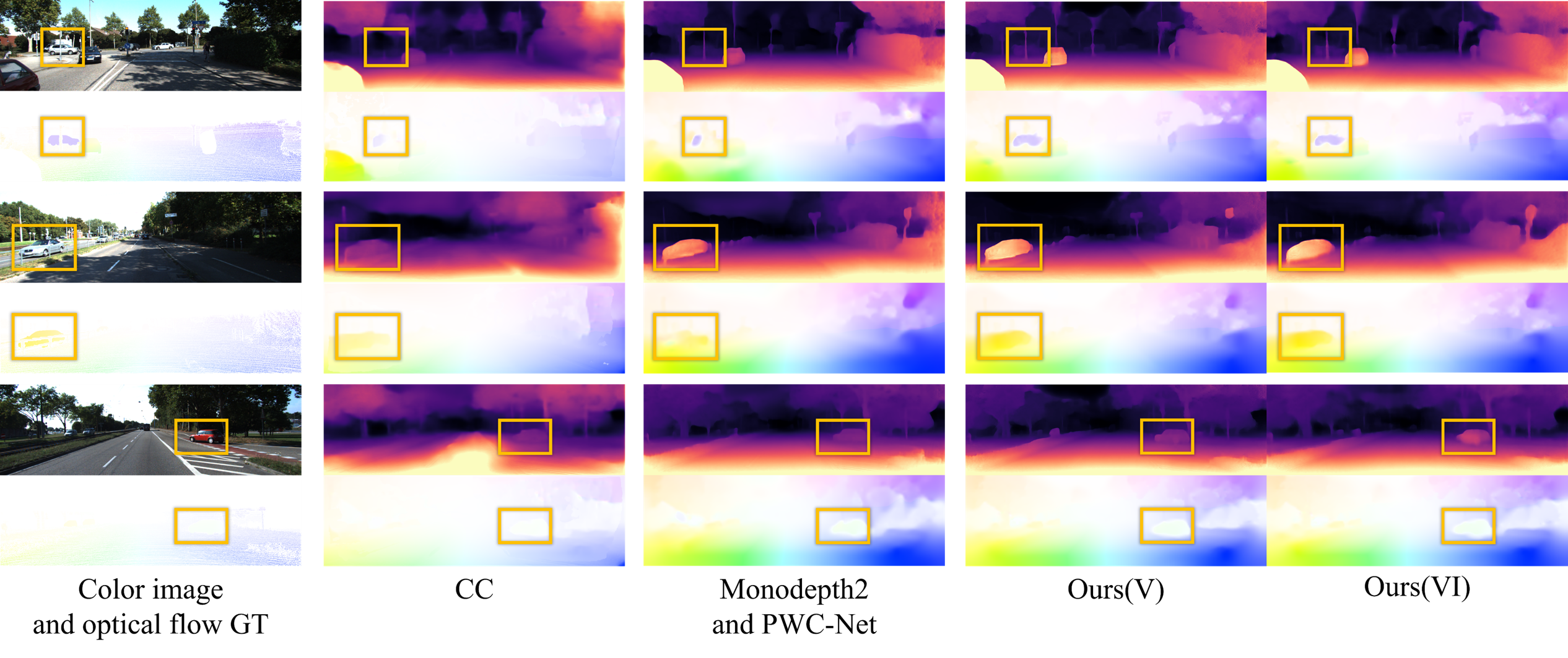
Figure 7: Depth and optical flow prediction illustration comparison between CC [30], monodepth2 [50]+PWC-Net [21], and our method (model V and VI). Column (a) shows the target image and its optical flow GT. Column (b), (c), and (d) shows the depth and optical flow prediction results of CC, monodepth2 and PWC-Net, and our method.

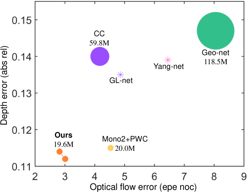
Figure 8: Bubble chart comparing the trade-off of depth estimation, optical flow prediction, and parameter mount between different methods. The horizontal and vertical axis represents optical flow prediction non-occluded pixels endpoint error and depth prediction absolute relative error, while the size of the bubbles shows the parameter mounts.

The comparisons of monocular depth and optical flow estimation between our approach and other methods are summarized in Tab. II, Fig. 7, and Fig. 8.

In Tab. II and Fig. 8, we take our models in experiment V and VI of Tab. I to compare with other baselines. Our models achieve better or comparable results for depth and optical flow estimation. Moreover, benefit from shared encoder and small components, our models contain small amount of parameters and thus achieve higher or comparable FPS. Moreover, as shown in Fig. 7, in both depth and optical flow prediction, our method achieves significant improvement of detecting vehicles.

V CONCLUSION

In this paper, we design a multi-task network that achieves mutual assistance between the two tasks of optical flow and depth prediction through bi-directional information interaction. Specifically, we design D2F and F2D modules for cross-domain information interaction and apply the EMA method to the training of the network. We further enhance the network’s ability to distinguish objects during multi-task prediction by the applying dual-head mechanism to the optical flow branch. Besides improving the mean accuracy of depth and optical flow prediction, our method significantly facilitates the ability to tell objects like road signs and vehicles from the scene. In the future, our work can be applied to the visual perception of autonomous vehicles and the navigation of surgical robots.

References

- [1] J. Janai, F. Güney, A. Behl, A. Geiger, et al., “Computer vision for autonomous vehicles: Problems, datasets and state of the art,” Foundations and Trends® in Computer Graphics and Vision, vol. 12, no. 1–3, pp. 1–308, 2020.
- [2] M. Pirvu, V. Robu, V. Licaret, D. Costea, A. Marcu, E. Slusanschi, R. Sukthankar, and M. Leordeanu, “Depth distillation: unsupervised metric depth estimation for uavs by finding consensus between kinematics, optical flow and deep learning,” in Proceedings of the IEEE/CVF Conference on Computer Vision and Pattern Recognition, 2021, pp. 3215–3223.
- [3] B. Huang, J.-Q. Zheng, A. Nguyen, D. Tuch, K. Vyas, S. Giannarou, and D. S. Elson, “Self-supervised generative adversarial network for depth estimation in laparoscopic images,” in International Conference on Medical Image Computing and Computer-Assisted Intervention. Springer, 2021, pp. 227–237.
- [4] J.-Q. Zheng, X.-Y. Zhou, C. Riga, and G.-Z. Yang, “Real-time 3-d shape instantiation for partially deployed stent segments from a single 2-d fluoroscopic image in fenestrated endovascular aortic repair,” IEEE Robotics and Automation Letters, vol. 4, no. 4, pp. 3703–3710, 2019.
- [5] M. Klodt and A. Vedaldi, “Supervising the new with the old: learning sfm from sfm,” in Proceedings of the European Conference on Computer Vision (ECCV), 2018, pp. 698–713.
- [6] N. Yang, R. Wang, J. Stuckler, and D. Cremers, “Deep virtual stereo odometry: Leveraging deep depth prediction for monocular direct sparse odometry,” in Proceedings of the European Conference on Computer Vision (ECCV), September 2018.
- [7] D. Eigen, C. Puhrsch, and R. Fergus, “Depth map prediction from a single image using a multi-scale deep network,” Advances in neural information processing systems, vol. 27, 2014.
- [8] I. Laina, C. Rupprecht, V. Belagiannis, F. Tombari, and N. Navab, “Deeper depth prediction with fully convolutional residual networks,” in 2016 Fourth international conference on 3D vision (3DV). IEEE, 2016, pp. 239–248.
- [9] B. Li, Y. Dai, and M. He, “Monocular depth estimation with hierarchical fusion of dilated cnns and soft-weighted-sum inference,” Pattern Recognition, vol. 83, pp. 328–339, 2018.
- [10] D. Eigen, C. Puhrsch, and R. Fergus, “Depth map prediction from a single image using a multi-scale deep network,” MIT Press, 2014.
- [11] A. Saxena, S. Min, and A. Y. Ng, “Make3d: Learning 3d scene structure from a single still image,” IEEE Transactions on Pattern Analysis and Machine Intelligence, 2008.
- [12] B. Huang, J.-Q. Zheng, A. Nguyen, C. Xu, I. Gkouzionis, K. Vyas, D. Tuch, S. Giannarou, and D. S. Elson, “Self-supervised depth estimation in laparoscopic image using 3d geometric consistency,” arXiv preprint arXiv:2208.08407, 2022.
- [13] R. Garg, V. K. Bg, G. Carneiro, and I. Reid, “Unsupervised cnn for single view depth estimation: Geometry to the rescue,” in European conference on computer vision. Springer, 2016, pp. 740–756.
- [14] C. Godard, O. Mac Aodha, and G. J. Brostow, “Unsupervised monocular depth estimation with left-right consistency,” in Proceedings of the IEEE conference on computer vision and pattern recognition, 2017, pp. 270–279.
- [15] B. Huang, J.-Q. Zheng, S. Giannarou, and D. S. Elson, “H-net: Unsupervised attention-based stereo depth estimation leveraging epipolar geometry,” in Proceedings of the IEEE/CVF Conference on Computer Vision and Pattern Recognition, 2022, pp. 4460–4467.
- [16] T. Zhou, M. Brown, N. Snavely, and D. G. Lowe, “Unsupervised learning of depth and ego-motion from video,” in Proceedings of the IEEE conference on computer vision and pattern recognition, 2017, pp. 1851–1858.
- [17] T. Zhou, S. Tulsiani, W. Sun, J. Malik, and A. A. Efros, “View synthesis by appearance flow,” in European conference on computer vision. Springer, 2016, pp. 286–301.
- [18] M. Xiong, Z. Zhang, W. Zhong, J. Ji, J. Liu, and H. Xiong, “Self-supervised monocular depth and visual odometry learning with scale-consistent geometric constraints,” in Proceedings of the Twenty-Ninth International Conference on International Joint Conferences on Artificial Intelligence, 2021, pp. 963–969.
- [19] B. K. Horn and B. G. Schunck, “Determining optical flow,” Artificial intelligence, vol. 17, no. 1-3, pp. 185–203, 1981.
- [20] Q. Chen and V. Koltun, “Full flow: Optical flow estimation by global optimization over regular grids,” in Proceedings of the IEEE conference on computer vision and pattern recognition, 2016, pp. 4706–4714.
- [21] D. Sun, X. Yang, M.-Y. Liu, and J. Kautz, “Pwc-net: Cnns for optical flow using pyramid, warping, and cost volume,” in Proceedings of the IEEE conference on computer vision and pattern recognition, 2018, pp. 8934–8943.
- [22] E. Ilg, N. Mayer, T. Saikia, M. Keuper, A. Dosovitskiy, and T. Brox, “Flownet 2.0: Evolution of optical flow estimation with deep networks,” in Proceedings of the IEEE conference on computer vision and pattern recognition, 2017, pp. 2462–2470.
- [23] Z. Teed and J. Deng, “Raft: Recurrent all-pairs field transforms for optical flow,” in European conference on computer vision. Springer, 2020, pp. 402–419.
- [24] N. Sundaram, T. Brox, and K. Keutzer, “Dense point trajectories by gpu-accelerated large displacement optical flow,” in European conference on computer vision. Springer, 2010, pp. 438–451.
- [25] Y. Wang, Y. Yang, Z. Yang, L. Zhao, P. Wang, and W. Xu, “Occlusion aware unsupervised learning of optical flow,” in Proceedings of the IEEE Conference on Computer Vision and Pattern Recognition, 2018, pp. 4884–4893.
- [26] S. Meister, J. Hur, and S. Roth, “Unflow: Unsupervised learning of optical flow with a bidirectional census loss,” in Thirty-Second AAAI Conference on Artificial Intelligence, 2018.
- [27] Y. Zou, Z. Luo, and J.-B. Huang, “Df-net: Unsupervised joint learning of depth and flow using cross-task consistency,” in Proceedings of the European conference on computer vision (ECCV), 2018, pp. 36–53.
- [28] Y. Chen, C. Schmid, and C. Sminchisescu, “Self-supervised learning with geometric constraints in monocular video: Connecting flow, depth, and camera,” in Proceedings of the IEEE/CVF International Conference on Computer Vision, 2019, pp. 7063–7072.
- [29] Y. Wang, P. Wang, Z. Yang, C. Luo, Y. Yang, and W. Xu, “Unos: Unified unsupervised optical-flow and stereo-depth estimation by watching videos,” in Proceedings of the IEEE/CVF Conference on Computer Vision and Pattern Recognition, 2019, pp. 8071–8081.
- [30] A. Ranjan, V. Jampani, L. Balles, K. Kim, D. Sun, J. Wulff, and M. J. Black, “Competitive collaboration: Joint unsupervised learning of depth, camera motion, optical flow and motion segmentation,” in Proceedings of the IEEE/CVF Conference on Computer Vision and Pattern Recognition, 2019, pp. 12 240–12 249.
- [31] G. Wang, C. Zhang, H. Wang, J. Wang, Y. Wang, and X. Wang, “Unsupervised learning of depth, optical flow and pose with occlusion from 3d geometry,” IEEE Transactions on Intelligent Transportation Systems, 2020.
- [32] Y. Cao, X. Zhang, F. Luo, P. Peng, and Y. Li, “Robust visual odometry using position-aware flow and geometric bundle adjustment,” arXiv preprint arXiv:2111.11141, 2021.
- [33] W. Zhao, S. Liu, Y. Shu, and Y.-J. Liu, “Towards better generalization: Joint depth-pose learning without posenet,” in Proceedings of the IEEE/CVF Conference on Computer Vision and Pattern Recognition, 2020, pp. 9151–9161.
- [34] A. Geiger, P. Lenz, and R. Urtasun, “Are we ready for autonomous driving? the kitti vision benchmark suite,” in 2012 IEEE conference on computer vision and pattern recognition. IEEE, 2012, pp. 3354–3361.
- [35] Z. Yin and J. Shi, “Geonet: Unsupervised learning of dense depth, optical flow and camera pose,” in Proceedings of the IEEE conference on computer vision and pattern recognition, 2018, pp. 1983–1992.
- [36] D. Yang, Z. Luo, P. Shang, and Z. Hu, “Unsupervised deep learning of depth, ego-motion, and optical flow from stereo images,” in 2021 9th International Conference on Traffic and Logistic Engineering (ICTLE). IEEE, 2021, pp. 51–56.
- [37] J. Xie, C. Lei, Z. Li, L. E. Li, and Q. Chen, “Video depth estimation by fusing flow-to-depth proposals,” in 2020 IEEE/RSJ International Conference on Intelligent Robots and Systems (IROS). IEEE, 2020, pp. 10 100–10 107.
- [38] Z. Yang, R. Simon, Y. Li, and C. A. Linte, “Dense depth estimation from stereo endoscopy videos using unsupervised optical flow methods,” in Annual Conference on Medical Image Understanding and Analysis. Springer, 2021, pp. 337–349.
- [39] V. Guizilini, K.-H. Lee, R. Ambrus, and A. Gaidon, “Learning optical flow, depth, and scene flow without real-world labels,” IEEE Robotics and Automation Letters, 2022.
- [40] D. Jia, K. Wang, S. Luo, T. Liu, and Y. Liu, “Braft: Recurrent all-pairs field transforms for optical flow based on correlation blocks,” IEEE Signal Processing Letters, vol. 28, pp. 1575–1579, 2021.
- [41] C. Chi, Q. Wang, T. Hao, P. Guo, and X. Yang, “Feature-level collaboration: Joint unsupervised learning of optical flow, stereo depth and camera motion,” in Proceedings of the IEEE/CVF Conference on Computer Vision and Pattern Recognition, 2021, pp. 2463–2473.
- [42] J. Hur and S. Roth, “Self-supervised monocular scene flow estimation,” in Proceedings of the IEEE/CVF Conference on Computer Vision and Pattern Recognition, 2020, pp. 7396–7405.
- [43] J. Chen, X. Yang, Q. Jia, and C. Liao, “Denao: Monocular depth estimation network with auxiliary optical flow,” IEEE transactions on pattern analysis and machine intelligence, vol. 43, no. 8, pp. 2598–2610, 2020.
- [44] A. Tarvainen and H. Valpola, “Mean teachers are better role models: Weight-averaged consistency targets improve semi-supervised deep learning results,” Advances in neural information processing systems, vol. 30, 2017.
- [45] C. Godard, O. Mac Aodha, and G. J. Brostow, “Unsupervised monocular depth estimation with left-right consistency,” in Proceedings of the IEEE conference on computer vision and pattern recognition, 2017, pp. 270–279.
- [46] J. Devlin, M. W. Chang, K. Lee, and K. Toutanova, “Bert: Pre-training of deep bidirectional transformers for language understanding,” 2018.
- [47] A. Vaswani, N. Shazeer, N. Parmar, J. Uszkoreit, L. Jones, A. Gomez, L. Kaiser, and I. Polosukhin, “Attention is all you need,” 06 2017.
- [48] J.-Q. Zheng, Z. Wang, B. Huang, N. H. Lim, and B. W. Papiez, “Residual aligner network,” arXiv preprint arXiv:2203.04290, 2022.
- [49] D. Eigen and R. Fergus, “Predicting depth, surface normals and semantic labels with a common multi-scale convolutional architecture,” in Proceedings of the IEEE international conference on computer vision, 2015, pp. 2650–2658.
- [50] C. Godard, O. Mac Aodha, M. Firman, and G. J. Brostow, “Digging into self-supervised monocular depth estimation,” in Proceedings of the IEEE/CVF International Conference on Computer Vision, 2019, pp. 3828–3838.
- [51] D. P. Kingma and J. Ba, “Adam: A method for stochastic optimization,” arXiv preprint arXiv:1412.6980, 2014.