Analytical solution of the disordered Tavis-Cummings model and its Fano resonances

Abstract

$\mathcal{N}$ emitters collectively coupled to a quantised cavity mode are described by the Tavis-Cummings model. We present complete analytical solution of the model in the presence of inhomogeneous couplings and energetic disorder. We derive the exact expressions for the bright and the dark sectors that decouple the disordered model and find that, in the thermodynamic limit, the energetic disorder transforms the bright sector to Fano’s model that can be easily solved. We thoroughly explore the effects of energetic disorder assuming a Gaussian distribution of emitter transition energies. We compare the Fano resonances in optical absorption and inelastic electron scattering both in the weak and the strong coupling regimes. We study the evolution of the optical absorption with an increase in the disorder strength and find that it changes the lower and upper polaritons to their broadened resonances that finally transform to a single resonance at the bare cavity photon energy, thus taking the system from the strong to the weak coupling regime. Interestingly, we learn that the Rabi splitting can exist even in the weak coupling regime while the polaritonic peaks in the strong coupling regime can represent almost excitonic states at intermediate disorder strengths. We also calculate the photon Green’s function to see the effect of cavity leakage and non-radiative emitter losses and find that the polariton linewidth exhibits a minimum as a function of detuning when the cavity leakage is comparable to the Fano broadening.

I Introduction

Cavity quantum electrodynamics (cavity QED) deals with the interaction of spatially confined quantised electromagnetic field and some form of matter excitations that can originate from a number of different systems, e.g., atoms Walther et al. (2006); Mivehvar et al. (2021), molecules Lidzey et al. (1998); Keeling and Kéna-Cohen (2020), quantum dots Kiraz et al. (2003); Stockklauser et al. (2017); Najer et al. (2019) and Bose-Einstein condensates Colombe et al. (2007); Brennecke et al. (2007). In microcavities, interesting many-body phenomena can arise as the photons mediate interaction Vaidya et al. (2018); Guo et al. (2019); Periwal et al. (2021) and coherence Georges et al. (2018) between the matter constituents and in turn acquire correlations among themselves even when they leak out Clark et al. (2020). In the strong coupling regime Dovzhenko et al. (2018), these systems host polaritons Basov et al. (2021) that have a hybrid matter-light character and, due to their technological prospects Kasprzak et al. (2006); Houck et al. (2012); Sanvitto and Kéna-Cohen (2016); Keeling and Kéna-Cohen (2020); Kravtsov et al. (2020); Moxley et al. (2021), have been extensively studied.

The minimal model to describe the cavity QED with multiple matter systems, or emitters as they are usually called, is the Tavis-Cummings (TC) model Tavis and Cummings (1968). The model can be analytically solved in the absence of disorder using the bright (symmetric) and dark (non-symmetric) states Ribeiro et al. (2018); Zeb (2021). However, in the presence of a disorder in the transition energies of the emitters, these states are not decoupled so this transformation is rendered useless and we resort to brute force numerical solutions Ćwik et al. (2016); Botzung et al. (2020); Du and Yuen-Zhou (2022). In some cases, the disorder can even invalidate the basic TC model and an extension is deemed necessary Blaha et al. (2022). In natural systems, on the one hand, disorder both in the transition energies and couplings is inevitable. On the other, a tuneable disorder can be realised in artificial systems Huang et al. (2019); Mazhorin et al. (2022). Thus, exploring the effects of disorder is important and solving the TC model analytically can be a significant step forward as it can provide us with an insight into the disordered cavity QED systems.

Although the TC model describes a wide range of systems, we illustrate our results here considering organic microcavities as an example. The transition energies of organic molecules usually have a distribution of width ${\sqrt{2}\times 0.1eV}$ Bässler (1981); Bässler et al. (1982); fno , which is a sizeable fraction of the typical Rabi splitting of $0.5eV$ Tropf and Gather (2018) in these systems. Furthermore, the distribution of orientations and positions of the molecules in the cavity translates to a disorder in their couplings to the cavity mode.

Organic polaritons have interesting properties, e.g., condensation and lasing at room temperature Kéna-Cohen and Forrest (2010); Plumhof et al. (2013); Keeling and Kéna-Cohen (2020). Their effect on materials’ properties, e.g., charge and energy transport Feist and Garcia-Vidal (2015); Hagenmüller et al. (2017); Schäfer et al. (2019); Zeb et al. (2020), and chemical reaction rates Thomas et al. (2019); Herrera and Spano (2016); Galego et al. (2016, 2017); Martínez-Martínez et al. (2018); Ebbesen (2016); Feist et al. (2017); Ribeiro et al. (2018) is also studied recently. Besides the polaritons, we have a large number of dark states in such systems Ribeiro et al. (2018); Kéna-Cohen and Yuen-Zhou (2019), that also play important role in various processes of interest, e.g., catalysis Du and Yuen-Zhou (2022). While the dark states were initially thought to be only a reservoir of incoherent excitations Agranovich et al. (2002, 2003), they are now well appreciated for their coherence and delocalised nature Gonzalez-Ballestero et al. (2016); Hu et al. (2018); Pandya et al. (2022). Although, the dark states do not couple to the light, they can still be excited optically indirectly by exciting polaritons or higher energy emitter states. In addition, the electrical excitation predominantly creates the dark states due to their large density of states. The dark states can relax to the lower polariton state, which is important for creating large polariton population for condensation and lasing for instance, and their dynamics has been studied extensively del Pino et al. (2018); Groenhof et al. (2019); Sommer et al. (2021); Eizner et al. (2019); Polak et al. (2020); Yu et al. (2021); Mewes et al. (2020); Wersäll et al. (2019); Xiang et al. (2019). The effect of disorder on the localisation of the dark state has also been numerically studied recently Botzung et al. (2020). Due to their hugely important role in organic microcavities and other cavity QED systems, it is desired to know their exact form under realistic conditions, which can lead to a significant development of analytical methods.

Since real systems are often weakly coupled to their environment, the resulting homogeneous broadening of the cavity and molecular states is inherited by the polariton states, and can be treated using open quantum system approaches—master equations—or phenomenologically with the Green’s functions Thompson et al. (1992); Herrera and Spano (2017); Zhang and Zhang (2021) (or an equivalent quantum control method Dong et al. (2022)). In fact, to obtain the optical absorption spectrum, the Green’s functions can exactly treat the energetic disorder or the inhomogeneous broadening as well Mazhorin et al. (2022); Gera and Sebastian (2022), as we will later show in this article. (Nevertheless, it has also been used to find an approximate solution by neglecting the effect of energetic disorder on the light-matter coupling strength Ćwik et al. (2016).) However, only the photon Green’s function can be computed this way, which alone cannot describe the eigenstates of the system, thus severely limiting the scope of the previous studies Ćwik et al. (2016); Mazhorin et al. (2022); Gera and Sebastian (2022); Dong et al. (2022).

The exact numerical diagonalisation, another method that is simple and usually effective, has its own shortcoming. In a clean system with identical emitters, studying the collective effects in the thermodynamic limit is possible as the typical size that is considered large enough is $\mathcal{N}=20$, where $\mathcal{N}$ is the number of emitters. However, in an energetically disordered system, a realistically smooth distribution of states that converges the results requires $\mathcal{N}\gg 10^{6}$, which is computationally intractable considering that all eigenstates of the Hamiltonian are to be computed. This is the reason that exact diagonalisation in such cases would even fail to capture the features in the optical spectrum that are given by the photon Green’s function in the thermodynamic limit.

What is so important in the thermodynamic limit of the energetically disordered system that has not yet been understood? It is the emergence of the Fano’s model Fano (1961), which can only be found if the Hamiltonian is first decoupled into its exact bright and dark subspaces. Fano’s model describes the interaction of a discrete or localised state to a continuous band and exhibits Fano resonances Fano (1961); Miroshnichenko et al. (2010); Kamenetskii et al. (2018); Cao et al. (2020); Zeb (2022). It gives a characteristic asymmetric lineshape in excitation spectra that finds applications Limonov (2021) in sensing and switching devices Nozaki et al. (2013); Stern et al. (2014). It is ubiquitous in physical systems  Zhang et al. (2006, 2008); Tang et al. (2010); Ott et al. (2013); Luo et al. (2004); Zielinski et al. (2015); Wang et al. (2017); Limonov et al. (2017) but, being a coherent phenomenon, finding it in a disordered system Poddubny et al. (2012); Silevitch et al. (2019) is not common. The Fano’s model has always been applied in the weak coupling regime but, as we will shortly see, it is also relevant in the strong coupling regime Zeb (2022).

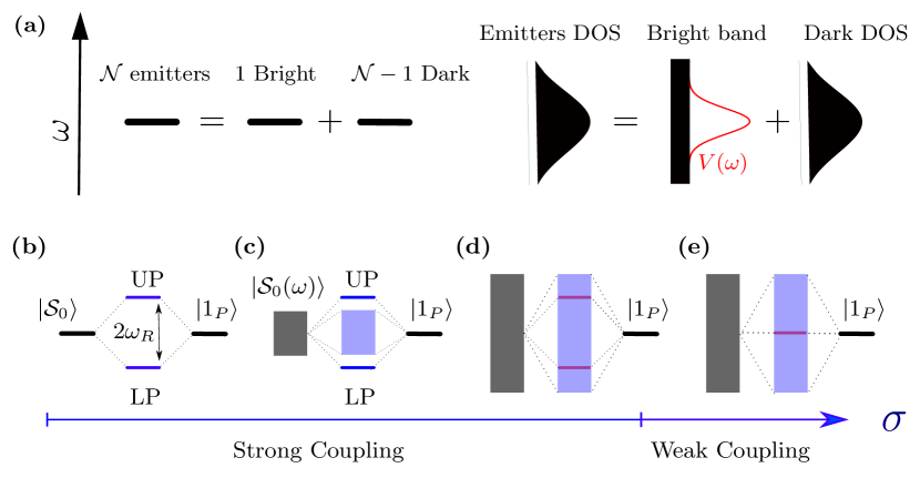
Figure 1: Effect of energetic disorder in the thermodynamic limit. (a) Bright (permutation symmetric) and dark (non-symmetric) states. In the absence of energetic disorder (left), $\mathcal{N}$ emitters form a single bright state and ${\mathcal{N}-1}$ dark states. In the presence of energetic disorder (right), where the density of states (DOS) forms a localised distribution, such bright-dark decoupling occurs at all energies separately, which produces a non-degenerate continuum of bright states (flat DOS) and a distribution of dark states. The coupling of the bright band to the cavity mode $V(\omega)$ equals the square root of the emitter DOS. (b-e) The eigenstates of the system formed by the coupling between the bright state ${\ket{\mathcal{S}_{0}}}$ or band ${\ket{\mathcal{S}_{0}(\omega)}}$ and the cavity photon state ${\ket{1_{P}}}$ . Without energetic disorder (b), upper and lower polaritons (UP, LP) are formed. With energetic disorder (c-e), we have a continuum of eigenstates at the original bright band energies but the true polariton states exist only at small disorder (c). At intermediate disorder, we have polariton’s Fano resonances (d) that transform to the photon’s Fano resonance (e) at large disorder strengths.

Here, we consider the Tavis-Cummings model with disorder both in emitter energies and their couplings to the cavity mode. We derive the exact expressions for the bright and the dark states that span the two decoupled subspaces of the model. We show that, in the thermodynamic limit, the bright states of the disordered system form a non-degenerate band whose interaction with the cavity mode gives the Fano’s model that can be exactly solved. Figure 1 illustrates the formation of the bright band and the nature of the eigenstates of the system at varying levels of the disorder strength. In Fig. 1(a), when $\mathcal{N}$ emitters have the same transition energy, their states can be transformed to give a single bright state ${\ket{\mathcal{S}_{0}}}$ that couples to the cavity and ${\mathcal{N}-1}$ dark states that are decoupled, hence the names. However, when the emitter energies form a distribution, a similar transformation at every energy produces bright and dark states at that energy, decoupling the dark sector completely and forming a non-degenerate band of bright states ${\ket{\mathcal{S}_{0}(\omega)}}$ with flat density of states (DOS). The eigenstates of the system in the single excitation space are formed by the coupling between ${\ket{\mathcal{S}_{0}}}$ or ${\ket{\mathcal{S}_{0}(\omega)}}$ and the cavity photon state ${\ket{1_{P}}}$ as shown in Fig. 1(b-e), where different scenarios that give polaritons [Fig. 1(b,c)], their Fano resonances [Fig. 1(d)] and the photon’s Fano resonance [Fig. 1(e)] are illustrated, which result from progressively increasing the energetic disorder $\sigma$ that takes the system from the strong coupling regime to the weak coupling regime. Our calculations suggest that the polaritons are a manifestation of the Fano resonances at weak disorder. Further, we show that the Rabi splitting or the anticrossing in the optical spectra does not have to correspond to the polaritons, they should also be seen when the corresponding Fano resonances are better thought of as matter states with strong optical absorption.

For completeness, we also consider the effect of losses on the the optical response of the system and compute the exact photon Green’s function that encodes it. We explore the effect of cavity and emitter losses on the optical absorption spectrum and find that, in organic microcavities, it should exhibit a minimum in the polariton linewidth around zero detuning. While preparing for the revised version of this manuscript, we found another work with some overlap Gera and Sebastian (2022).

The organisation of this article is as follows. The decoupling of the TC model into its bright and dark spaces is presented in sec. II, where sec. II.1 considers $\mathcal{N}$ identical emitters, sec. II.2 includes disorder in the couplings only, while sec. II.3 also takes account of energetic disorder. Section III contains the results related to the Fano’s model. The emergence of the Fano’s model and its solution in two possible scenarios [shown in Fig. 1(c,d)] are given in sec. III.1. Fano resonances in two types of excitation spectra—optical absorption and inelastic electron scattering—are presented in sec. III.2 both in the weak and strong coupling regimes. Section IV explores the effects of energetic disorder, where sec. IV.1 considers the Rabi splitting and the nature of the eigenstates, sec. IV.2 discusses the differences from a homogeneous broadening, and sec. IV.3 analyse the Fano broadening of polaritons. Finally, the effects of losses are described in sec. V, where the photon Green’s function is used to study the polariton lineshape and linewidth as well as the role of the distribution of emitters’ energies.

II Model and its solution

Consider $\mathcal{N}$ two-level emitters coupled to a common cavity mode. The Hamiltonian of this system in the rotating wave approximation Scully and Zubairy (1997) is given by

$$\mathcal{\hat{H}}=\omega_{c}\hat{a}^{\dagger}\hat{a}+\sum_{i=1}^{\mathcal{N}}\Big{\{}\epsilon_{i}\hat{\sigma}_{i}^{+}\hat{\sigma}_{i}^{-}+g_{i}(\hat{a}^{\dagger}\hat{\sigma}^{-}_{i}+\hat{\sigma}^{+}_{i}\hat{a})\Big{\}},$$ (1)

where $\omega_{c}$ is the energy of a cavity photon, $\hat{a}^{\dagger},\hat{a}$ are its creation and annihilation operators, and $\sigma_{i}^{\pm}$ are raising and lowering operators for the $i$th emitter that has transition energy $\epsilon_{i}$ and couples to the cavity mode with strength $g_{i}$. Both $g_{i}$ and $\epsilon_{i}$ are randomly distributed according to some probability functions. $\mathcal{\hat{H}}$ commutes with the excitation number ${\hat{\mathcal{N}}_{ex}=\hat{a}^{\dagger}\hat{a}+\sum_{i}^{\mathcal{N}}\hat{\sigma}^{+}_{i}\hat{\sigma}^{-}_{i}}$, which allows its diagonalisation in an eigenspace of $\hat{\mathcal{N}}_{ex}$. We will focus on the single excitation subspace in this article.

In the following sections, we describe the decoupling of the emitters’ Hilbert space into bright and dark sectors, where the bright sector couples to the cavity mode but the dark sector does not.

II.1 Identical Emitters

For identical emitters, i.e., when ${\epsilon_{i}=\epsilon}$ and ${g_{i}=g}$ for all $i$, the solution is already well known. In this case, a unitary transformation to the symmetric (bright) and non-symmetric (dark) superpositions of the emitter states block-diagonalises the TC model in the single excitation space. The bright state is created by

$$\hat{\mathcal{S}}^{+}_{0} \equiv \frac{1}{\sqrt{\mathcal{N}}}\sum_{i=1}^{\mathcal{N}}\hat{\sigma}_{i}^{+},$$ (2)

and produces the two polariton states due to its coupling to the cavity mode, which are given by,

$$\hat{\Psi}_{UP}^{+} =\cos\theta\hat{a}^{\dagger}+\sin\theta\hat{\mathcal{S}}^{+}_{0},$$ (3)

$$\hat{\Psi}_{LP}^{+} =\sin\theta\hat{a}^{\dagger}-\cos\theta\hat{\mathcal{S}}^{+}_{0},$$ (4)

$$\omega_{UP} =\frac{1}{2}(-\delta+\sqrt{\delta^{2}+4\omega_{R}^{2}}),$$ (5)

$$\omega_{LP} =-\frac{1}{2}(\delta+\sqrt{\delta^{2}+4\omega_{R}^{2}}),$$ (6)

$$2\theta =\tan^{-1}(2\omega_{R}/\delta),$$ (7)

where $\delta=\omega_{c}-\epsilon$ and $\hat{\Psi}_{UP/LP}^{+}$ create the polaritonic states at energies $\omega_{UP/LP}$.

For the non-symmetric or dark states, being a degenerate manifold (at the bare exciton energy $\epsilon$), there is no unique representation and one can choose any complete set as basis states for the dark space. Usually, a set of delocalised discrete Fourier transform states is used, given by

$$\hat{\tilde{\mathcal{S}}}^{+}_{k} \equiv \frac{1}{\sqrt{\mathcal{N}}}\sum_{n=1}^{\mathcal{N}}e^{i2\pi kn/\mathcal{N}}\hat{\sigma}_{n}^{+},~{}k\in[1,\mathcal{N}-1].$$

In case of inhomogeneous couplings, (i.e., when a disorder in the couplings exists), these states no longer represent the dark sector. Here, we present another set that can be easily modified in such a case.

Inspired from the maximally localised dark state,

$$\hat{\mathcal{S}}^{+}_{\mathcal{N}-1} \equiv \sqrt{\frac{\mathcal{N}-1}{\mathcal{N}}}\hat{\sigma}_{\mathcal{N}}^{+}-\frac{1}{\sqrt{\mathcal{N}(\mathcal{N}-1)}}\sum_{i=1}^{\mathcal{N}-1}\hat{\sigma}_{i}^{+},$$

that is fairly known and is localised at site $\mathcal{N}$, we can focus on how it turns out to be orthogonal to the bright state $\hat{\mathcal{S}}^{+}_{0}$. We note that the contribution from the $\mathcal{N}$th site is exactly cancelled by the sites $1$ to $\mathcal{N}-1$. Designing another dark state on the same pattern to ensure its orthogonalisation to $\hat{\mathcal{S}}^{+}_{\mathcal{N}-1}$, we obtain $\hat{\mathcal{S}}^{+}_{\mathcal{N}-2}$ that is maximally localised on emitter $\mathcal{N}-1$ but has zero component along $\hat{\sigma}_{\mathcal{N}}^{+}$, i.e., on the site $\mathcal{N}$. Repeating this process, we construct an orthonormal representation for the dark states where different dark states tend to localise on different molecules, albeit to a varying degree, given by Zeb and Masood (2021)

$$\hat{\mathcal{S}}^{+}_{j} \equiv \frac{1}{\sqrt{j(j+1)}}\left(\sum_{i=1}^{j}\hat{\sigma}_{i}^{+}-j\hat{\sigma}_{j+1}^{+}\right),$$ (8)

where ${j\in[1,\mathcal{N}-1]}$.

II.2 Only off-diagonal disorder

It is well known that when a disorder in the couplings exists, $\hat{\mathcal{S}}^{+}_{0}$ modifies to

$$\hat{\mathcal{S}}^{+}_{0} \equiv \frac{1}{G_{\mathcal{N}}}\sum_{i=1}^{\mathcal{N}}g_{i}\hat{\sigma}_{i}^{+},$$ (9)

where ${G_{\mathcal{N}}^{2}\equiv\sum_{i=1}^{\mathcal{N}}g_{i}^{2}}$. However, exact expressions for the dark states are not known. As we mentioned in the previous section, we modify the maximally localised states to obtain just that. These can be obtained by following the changes in $\hat{\mathcal{S}}^{+}_{0}$ and imposing the orthogonalisation of the dark states to this bright state. That is, try

$$\hat{\mathcal{S}}^{+}_{j} \equiv \alpha_{j}\left(\sum_{i=1}^{j}g_{i}\hat{\sigma}_{i}^{+}-\beta_{j}\hat{\sigma}_{j+1}^{+}\right),$$

and impose $\braket{GS}{\hat{\mathcal{S}}^{-}_{0}\hat{\mathcal{S}}^{+}_{j}}{GS}=0$, where $\ket{GS}$ is the ground state of the emitters. This gives, ${\beta_{j}=G_{j}^{2}/g_{j+1}}$, and then normalisation ${\braket{GS}{\hat{\mathcal{S}}^{-}_{j}\hat{\mathcal{S}}^{+}_{j}}{GS}=1}$ gives ${\alpha_{j}=g_{j+1}/(G_{j}G_{j+1})}$. We thus obtain,

$$\hat{\mathcal{S}}^{+}_{j} \equiv\frac{g_{j+1}}{G_{j}G_{j+1}}\sum_{i=1}^{j}g_{i}\hat{\sigma}_{i}^{+}-\frac{G_{j}}{G_{j+1}}\hat{\sigma}_{j+1}^{+}.$$ (10)

II.3 Fully disordered

Due to the presence of disorder in the diagonal terms in $\mathcal{\hat{H}}$, the above transformations no longer work. However, as we show below, the exact bright and dark subspaces still do exist and it is still possible to block diagonalise $\mathcal{\hat{H}}$. Even though the energies $\{\epsilon_{i}\}$ are randomly distributed, assuming their intrinsic linewidth $\gamma$ to be negligible for the moment, we can count the number of states at any given energy and make bright and dark sectors for every energy level. Indexing these energy “levels” in ascending order, let’s take $K_{n}$ to be the degeneracy of the $n$th level at energy $\omega_{n}$. Relabelling the emitters ${i\to n,i_{n}}$ with $i_{n}\in[1,K_{n}]$ and dropping the subscript for brevity, ${\epsilon_{i}\to\omega_{n,i}}$, ${g_{i}\to g_{n,i}}$, and ${\sigma^{\pm}_{i}\to\sigma^{\pm}_{n,i}}$. This allows us to make the bright and the dark states for every level, similar to Eqs. 9-10. For $n$th degenerate level, we have

$$\hat{\mathcal{S}}^{+}_{n,0} \equiv\frac{1}{G_{n,K_{n}}}\sum_{i=1}^{K_{n}}g_{n,i}\hat{\sigma}_{n,i}^{+},$$ (11)

$$\hat{\mathcal{S}}^{+}_{n,j} \equiv\frac{g_{n,j+1}}{G_{n,j}G_{n,j+1}}\sum_{i=1}^{j}g_{n,i}\hat{\sigma}_{n,i}^{+}-\frac{G_{n,j}}{G_{n,j+1}}\hat{\sigma}_{n,j+1}^{+},$$ (12)

where ${j\in[1,K_{n}-1]}$ and ${G_{n,l}^{2}=\sum_{i=1}^{l}g_{n,i}^{2}}$. For the non-degenerate levels, only a bright state $\hat{\mathcal{S}}^{+}_{n,0}=\hat{\sigma}_{n,1}^{+}$ exists. Taking $N$ as the number of the bright states or the number of levels, $\mathcal{\hat{H}}$ can be written as ${\mathcal{\hat{H}}=\mathcal{\hat{H}}_{B}+\mathcal{\hat{H}}_{D}}$ where

$$\mathcal{\hat{H}}_{B}=\omega_{c}\hat{a}^{\dagger}\hat{a}+\sum_{n=1}^{N}\omega_{n}\hat{\mathcal{S}}^{+}_{n,0}\hat{\mathcal{S}}^{-}_{n,0}\\ +\sum_{n=1}^{N}G_{n,K_{n}}\left[\hat{a}\hat{\mathcal{S}}^{+}_{n,0}+\hat{a}^{\dagger}\hat{\mathcal{S}}^{-}_{n,0}\right],$$ (13)

$$~{}~{}~{}\mathcal{\hat{H}}_{D} =\sum_{n=1}^{N}\omega_{n}\sum_{j=1}^{K_{n}-1}\hat{\mathcal{S}}^{+}_{n,j}\hat{\mathcal{S}}^{-}_{n,j},$$ (14)

where $\mathcal{\hat{H}}_{D}$ is again already diagonal, and there are ${\mathcal{N}_{D}=\sum_{n=1}^{N}(K_{n}-1)=\mathcal{N}-N}$ dark states in total. Thus, to completely solve the disordered TC model, all that is left is the diagonalisation of $\mathcal{\hat{H}}_{B}$ above.

$\mathcal{\hat{H}}_{B}$ can be diagonalised numerically. The size of the bright space could be negligibly small compared to the full space, i.e., $N\lll\mathcal{N}$. For instance, even at $\mathcal{N}=10^{23}$, $N$ could be taken as small as ${\sim 10^{2}-10^{3}}$ for most realistic situations without compromising the thermodynamic limit. However, probably the best outcome of our approach is that, at large $\mathcal{N}$, when $\{\omega_{n}\}$ forms a continuous band, following Fano Fano (1961), analytical solution of $\mathcal{\hat{H}}_{B}$ can also be found, as follows.

III Emergence of Fano’s model

In the thermodynamic limit, $\mathcal{N}\to\infty$, we can consider the continuous limit for the bright band. Taking ${G_{n,K_{n}}^{2}\to V(\omega)^{2}d\omega}$,

$$V(\omega)^{2}d\omega =K(\omega)d\omega\int dgP_{c}(g)g^{2},$$

$$=\mathcal{N}P(\omega)d\omega\braket{g^{2}},$$ (15)

where $P_{c}(g)$ and $P(\omega)$ are distribution functions for couplings and energies. Note that as long as we get the same value for $\braket{g^{2}}$, the specific form of $P_{c}(g)$ does not matter. Taking ${\omega_{R}^{2}\equiv\sum_{n}G_{n,K_{n}}^{2}}$ and noting that $\int{P(\omega)d\omega}=1$, we can now write, $\omega_{R}^{2}=\int{V(\omega)^{2}d\omega}=\mathcal{N}\braket{g^{2}}$, which can be compared back to Eq. 15 above to write

$$V(\omega)=\omega_{R}\sqrt{P(\omega)}.$$ (16)

Thus, the continuous limit of $\mathcal{\hat{H}}_{B}$ in Eq. 13 becomes,

$$\mathcal{\hat{H}}_{B}=\omega_{c}\hat{a}^{\dagger}\hat{a}+\int\omega\hat{\mathcal{S}}^{+}_{0}(\omega)\hat{\mathcal{S}}^{-}_{0}(\omega)d\omega\\ +\int V(\omega)\left[\hat{a}\hat{\mathcal{S}}^{+}_{0}(\omega)+\hat{a}^{\dagger}\hat{\mathcal{S}}^{-}_{0}(\omega)\right]d\omega.$$ (17)

III.1 Fano’s model: $\mathcal{\hat{H}}_{B}$ in ${N_{ex}=1}$ subspace

There are three ingredients in the Fano’s model Fano (1961): (i) a discrete state interacting with a (ii) continuum of states that form the eigenstates of the system to which (iii) transition from another discrete state [uncoupled to (i) and (ii)] is to be explored. Since $N_{ex}$ is a conserved quantiy, $\mathcal{\hat{H}}_{B}$ is decoupled in subspaces with different $N_{ex}$. In the following we show that $\mathcal{\hat{H}}_{B,1_{ex}}$ — $\mathcal{\hat{H}}_{B}$ in $N_{ex}=1$ subspace — consists of (i) and (ii), whereas the transitions from the sole eigenstate of $\mathcal{\hat{H}}_{B,0_{ex}}$ (the ground state of the full system) to the eigenstates of $\mathcal{\hat{H}}_{B,1_{ex}}$ should give the Fano resonances.

In the single excitation subspace we can either have a cavity photon or a molecular excitation of the bright band. The corresponding states are ${\ket{1_{P}}\equiv\hat{a}^{\dagger}\ket{vac}}$ and ${\ket{\mathcal{S}_{0}(\omega)}\equiv\hat{\mathcal{S}}^{+}_{0}(\omega)\ket{vac}}$, where ${\ket{vac}=\ket{0_{P}}\otimes\ket{GS}}$ is the ground state of the full system that constitutes the subspace with zero excitation ${N_{ex}=0}$. So projecting $\mathcal{\hat{H}}_{B}$ to ${N_{ex}=1}$ subspace gives

$$\mathcal{\hat{H}}_{B,1_{ex}}=\omega_{c}\ket{1_{P}}\bra{1_{P}}+\int\omega\ket{\mathcal{S}_{0}(\omega)}\bra{\mathcal{S}_{0}(\omega)}d\omega\\ +\int V(\omega)\left(\frac{}{}\ket{1_{P}}\bra{\mathcal{S}_{0}(\omega)}+\ket{\mathcal{S}_{0}(\omega)}\bra{1_{P}}\right)d\omega.$$ (18)

We can see that $\mathcal{\hat{H}}_{B,1_{ex}}$ describes the interaction of a localised state ${\ket{1_{P}}}$ with a continuum ${\ket{\mathcal{S}_{0}(\omega)}}$. This model has been solved by Fano long ago Fano (1961) to explain the resonance bearing his name that occurs at small $V(\omega)$. Due to its relevance to the disordered TC model as shown above, we thoroughly explore this model in the strong coupling regime elsewhere Zeb (2022) where the continuum bandwidth $W$ is assumed to be the largest energy scale and all eigenstates lie within it. In real systems, e.g., organic microcavities, however, the distribution $P(\omega)$ is non-zero only in a finite energy window, which determines the bandwidth $W$ of the bright states. So the following two scenarios are possible for the eigenstates of $\mathcal{\hat{H}}_{B,1_{ex}}$ in general.

III.1.1 Small bandwidth: polaritons outside the continuum

At $W\lesssim 2\omega_{R}$, depending on the cavity detuning from the centre of $V(\omega)$, we can have one or two polaritons as discrete states outside the bright band, along with a continuum of eigenstates at the original bright band energies, as shown in Fig. 1(c). These eigenstates can be easily calculated, see Appendix VIII.1.

Assuming $\ket{{\Phi}(\omega)}$ represents the discrete eigenstates of $\mathcal{\hat{H}}_{B,1_{ex}}$ outside the bright band at energy $\omega={\tilde{\omega}}$, we find that

$$\ket{{\Phi}(\tilde{\omega})}=\ket{1_{P}}+\int{\frac{V(\omega^{\prime})}{{\tilde{\omega}}-\omega^{\prime}}\ket{\mathcal{S}_{0}(\omega^{\prime})}d\omega^{\prime}},$$ (19)

where the integration is over the bright band and the normalisation is left on purpose. The associated eigenvalues ${\tilde{\omega}}$ are given by the roots of

$${\tilde{\omega}}-\omega_{c}-F({\tilde{\omega}})=0$$ (20)

where

$$F({\tilde{\omega}}) =\int{\frac{V(\omega^{\prime})^{2}}{{\tilde{\omega}}-\omega^{\prime}}d\omega^{\prime}}.$$ (21)

Note that there is no singularity in the above integral as, by definition, ${\omega^{\prime}\neq{\tilde{\omega}}}$ in this case.

The roots of Eq. 20 can also lie within the bright continuum where $F(\omega)$ would be the principal value ($p.v.$) of the integral in Eq. 21. There can be up to three roots in the strong coupling case Zeb (2022) that can be named after the states they belong to in the extreme cases of weak and strong coupling regimes by considering a localised distribution $P(\omega)$ [remember that ${V(\omega)=\omega_{R}\sqrt{P(\omega)}}$]. If the width of $P(\omega)$ is taken to be $\sigma$, then at ${\sigma/\omega_{R}\gg 1}$ we will only have a single root ${{\tilde{\omega}}_{c}}$ at (or near) the cavity photon energy, while in the opposite case ${\sigma/\omega_{R}\ll 1}$ two more roots ${\tilde{\omega}}_{LP}$ and ${\tilde{\omega}}_{UP}$ exist at the lower and upper polariton energies. ${\tilde{\omega}}_{LP}$ and ${\tilde{\omega}}_{UP}$ can be inside the continuum or outside it. When inside, the corresponding states $\ket{{\Phi}(\tilde{\omega}_{LP})}$ and $\ket{{\Phi}(\tilde{\omega}_{UP})}$ are still eigenstates of $\mathcal{\hat{H}}_{B,1_{ex}}$ and produce polariton’s Fano resonances. This will be explained in the following when we discuss the structure of the continuum eigenstates.

The eigenstates of $\mathcal{\hat{H}}_{B,1_{ex}}$ within the bright continuum have already been calculated by Fano Fano (1961), where he correctly handled the singularities involved. Assuming $\ket{{\Psi}(\omega)}$ is such an eigenstate at energy $\omega$, we can write it as a superposition (Appendix VIII.1),

$$\ket{{\Psi}(\omega)}=\frac{\sin\Delta(\omega)}{\pi V(\omega)}\ket{{\Phi}(\omega)}-\cos\Delta(\omega)\ket{\mathcal{S}_{0}(\omega)},$$ (22)

where

$$\Delta(\omega) =-\arctan\left[\frac{\pi V(\omega)^{2}}{\omega-\omega_{c}-F(\omega)}\right].$$ (23)

The significance of the state $\ket{{\Phi}(\omega)}$ can now be appreciated further by noting the sine and cosine terms in the coefficients of the two component states in this expression. For a physical process that can excite the system from $\ket{vac}$ state to the eigenstate $\ket{{\Psi}(\omega)}$, there are two transition paths available—via $\ket{{\Phi}(\omega)}$ and $\ket{\mathcal{S}_{0}(\omega)}$ components—that can interfere if the corresponding amplitudes are finite for the two. This becomes quite interesting at the roots of Eq. 20 ${\tilde{\omega}}$ inside the continuum, where the phase ${\Delta(\omega)}$ jumps between $\pm\pi/2$ and, since sine and cosine functions have opposite parity, the two paths interfere constructively on one side of the root and destructively on the other side, leading to an asymmetric lineshape there. This is the Fano resonance that will be discussed later in sec. III.2. Since $\Delta=\pm\pi/2$ at ${\tilde{\omega}}$, ${\sin\Delta=\pm 1,\cos\Delta=0}$ there, and ${\ket{{\Psi}(\tilde{\omega})}=\ket{{\Phi}(\tilde{\omega})}/\pi V({\tilde{\omega}})}$ showing that $\ket{{\Phi}(\tilde{\omega})}$ also represents the eigenstates inside the continuum at ${{\tilde{\omega}}_{c},{\tilde{\omega}}_{LP},{\tilde{\omega}}_{UP}}$. In the weak coupling case, when only a single root ${\tilde{\omega}}_{c}$ exists, it will be called the photon’s Fano resonance. In the strong coupling case, if the roots ${\tilde{\omega}}_{LP}$ and/or ${\tilde{\omega}}_{UP}$ lie within the continuum, the resonances will be reminiscent of the discrete polariton states, and will hence be called polariton’s Fano resonances.

III.1.2 Large bandwidth: polaritons inside the continuum

At $W\gtrsim 2\omega_{R}$, we do not have any discrete polariton eigenstates because all roots of Eq. 20 lie within the bright band, as shown in Fig. 1(d,e). In this case, all eigenstates are described by $\ket{{\Psi}(\omega)}$ in Eq. 22. This completes the solution of the disordered TC model in the thermodynamic limit for a generic distribution $P(\omega)$.

An interesting situation arises when a polaritonic root ${{\tilde{\omega}}={\tilde{\omega}}_{LP/UP}}$ lies inside the bright band but the coupling ${V(\omega)\to 0}$ around its position. In such a case, ${\Delta(\omega)\to 0}$ at ${\omega\neq\tilde{\omega}}$, but ${\Delta(\tilde{\omega})\to\pm\pi/2}$ still holds. So, ${\ket{{\Psi}(\omega)}\to\ket{\mathcal{S}_{0}(\omega)}}$ at ${\omega\neq\tilde{\omega}}$, and ${\ket{\Psi(\tilde{\omega})}\propto\ket{\Phi(\tilde{\omega})}/V(\tilde{\omega})}$ as always. This observation can be used to unify the above two cases of small and large bandwidth into the latter, by extending the bright band on either side and simultaneously reducing the coupling ${V(\omega)\to 0}$ in the extended region. Considering that ${V(\omega)}$ is sharply localised naturally as ${V(\omega)^{2}=P(\omega)}$ can be assumed to be a Gaussian distribution for energetic disorder in real systems, the above trick will be used henceforth and $W$ will be assumed to be the largest energy scale.

Let’s take

$$P(\omega)=\frac{1}{\sqrt{2\pi}\sigma}e^{-\omega^{2}/2\sigma^{2}},$$ (24)

where $\sigma$ is the standard deviation that determines the width of the distribution and the mean energy ${\omega_{0}=\int{\omega P(\omega)d\omega}}$ is taken as a reference. We can now evaluate $F(\omega)$ in Eq. 21 to obtain

$$F(\omega) =\frac{\omega_{R}^{2}}{\sqrt{2\pi}\sigma}\times p.v.\int{\frac{e^{-\omega^{\prime 2}/2\sigma^{2}}}{\omega-\omega^{\prime}}d\omega^{\prime}},$$ (25)

$$F(\omega) =\pi\omega_{R}^{2}P(\omega)\operatorname{erfi}\left(\frac{\omega}{\sqrt{2}\sigma}\right),$$ (26)

$$\operatorname{erfi}(\omega) \equiv\operatorname{erf}(i\omega)/i,$$

where $\operatorname{erfi}$ is the imaginary error functions. The contribution of the tail of the Gaussian (that may not be present in real systems) in the above integral is negligible (even around ${\omega=\omega^{\prime}}$ on the tail — note that the $p.v.$ of the integral in Eq. 25 measures the asymmetry of $e^{-\omega^{2}/2\sigma^{2}}$ around $\omega$ in a small energy window as the denominator causes a suppression away from $\omega$).

The response of the system to an optical, electronic, or a hybrid excitation can now be evaluated. To illustrate the characteristic nature of the eigenstates, let’s first compare the inelastic electron scattering with the optical absorption. Later, we focus on the optical absorption as the main response function of the system.

III.2 Fano resonances

III.2.1 Optical absorption vs. inelastic electron scattering

For a generic process that can excite the system from $\ket{vac}$ to an eigenstate $\ket{\Psi(\omega)}$, the excitation probability normalised with the bare excitation probability of the continuum state $\ket{\mathcal{S}_{0}(\omega)}$ is given by the Fano formula  Fano (1961); Zeb (2022). Let’s assume $\hat{T}$ to be the operator that describes the excitation of molecules in an inelastic electron scattering event. Obtaining this spectrum in experiments on microcavities is likely to be the easiest when a gas of molecules is confined between the cavity mirrors or flows through them. In typical organic microcavities with active molecules in a solid film of thickness $\sim 100nm$ sandwiched between two plane mirrors, the exposed region of the film along its thickness can be probed. We can consider the excitation of the dark molecular states (eigenstates of $\mathcal{\hat{H}}_{D}$ in Eq. 14) as a background and focus on the bright band. The normalised probability for this process is given by Fano (1961); Zeb (2022),

$$\mathcal{M}(\omega) \equiv\frac{|\braket{\Psi(\omega)}{\hat{T}}{vac}|^{2}}{|\braket{\mathcal{S}_{0}(\omega)}{\hat{T}}{vac}|^{2}},$$

$$=\frac{(q+\epsilon)^{2}}{1+\epsilon^{2}},$$ (27)

where

$$\epsilon =\frac{\omega-\omega_{c}-F(\omega)}{\pi|V(\omega)|^{2}},$$

$$=\sqrt{\frac{2}{\pi}}\frac{\sigma}{\omega_{R}^{2}}e^{\omega^{2}/2\sigma^{2}}(\omega-\omega_{c})-\operatorname{erfi}(\omega/\sqrt{2}\sigma),$$ (28)

and the “asymmetry parameter” $q$ is given by

$$q =\frac{1}{\pi V(\omega)}\frac{\braket{\Phi(\omega)}{\hat{T}}{vac}}{\braket{\mathcal{S}_{0}(\omega)}{\hat{T}}{vac}},$$

$$=\frac{1}{\pi V(\omega)}p.v.\int{\frac{V(\omega^{\prime})d\omega^{\prime}}{\omega-\omega^{\prime}}},$$

$$=\operatorname{erfi}(\omega/2\sigma),$$ (29)

where we assumed the bare transition matrix element ${\braket{\mathcal{S}_{0}(\omega)}{\hat{T}}{vac}}$ is constant over the energy range of interest and used ${\braket{1_{P}}{\hat{T}}{vac}=0}$ as the electron scattering would not create cavity photons.

For the optical absorption in our hybrid system, however, the bare transition amplitude to the bright continuum is zero, i.e., ${\braket{\mathcal{S}_{0}(\omega)}{\hat{a}^{\dagger}}{vac}=0}$, where $\hat{a}^{\dagger}$ is the transition operator for this process. We thus use the unnormalised probability given by,

$$\mathcal{A}(\omega) \equiv|\braket{\Psi(\omega)}{\hat{a}^{\dagger}}{vac}|^{2},$$

$$=\frac{\omega_{R}^{2}P(\omega)}{[\omega-\omega_{c}-F(\omega)]^{2}+\pi^{2}\omega_{R}^{4}P(\omega)^{2}},$$ (30)

which is simply the photon spectral function. In the context of the weak coupling Fano resoance, the vanishing of ${\braket{\mathcal{S}_{0}(\omega)}{\hat{a}^{\dagger}}{vac}}$ also means that ${q=\infty}$, so the lineshape in the weak coupling regime is a Lorentzian whose width is given by the interaction strength Fano (1961); Zeb (2022). The above result is exact as long as there is no cavity leakage or non-radiative emitter losses. We will include these using Green’s function formalism later.

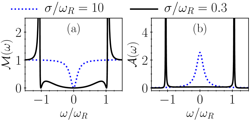
Figure 2: Fano resonances in (a) $\mathcal{M}(\omega)$ and (b) $\mathcal{A}(\omega)$ at $\sigma/\omega_{R}=10,0.3$ and $\omega_{c}=0$. Blue dotted lines are standard weak coupling Fano resonances (with asymmetry parameter ${q\simeq 0,\infty}$) while the black lines are their strong coupling Zeb (2022) counterparts.

III.2.2 Fano resonances in the weak and strong coupling regimes

Both $\mathcal{M}(\omega)$ and $\mathcal{A}(\omega)$ give information about the eigenstates of $\mathcal{\hat{H}}_{B,1_{ex}}$. However, their lineshapes are completely different due to the fact that they either excite the molecules or the cavity but not the both (as ${\braket{\mathcal{S}_{0}(\omega)}{\hat{a}^{\dagger}}{vac}=0=\braket{1_{P}}{\hat{T}}{vac}}$). Figure 2 shows $\mathcal{M}(\omega)$ and $\mathcal{A}(\omega)$ at ${\sigma/\omega_{R}=10,0.3}$ and ${\omega_{c}=0}$. At ${\sigma/\omega_{R}=10}$ (blue dotted curves), the system is in the weak coupling regime Zeb (2022) where we see the famous characteristic profiles around ${{\tilde{\omega}}_{c}=0}$ corresponding to ${q\simeq 0,\infty}$ — inverted Lorentzian dip in ${\mathcal{M}(\omega)}$ and a Lorentzian peak in ${\mathcal{A}(\omega)}$. In usual terms, the dip arises due to a destructive interference between two transition paths, one to the bare bright states $\ket{\mathcal{S}_{0}(\omega)}$ and the other to the modified (and broadened) discrete state $\ket{{\Phi}(\omega)}$ (that now has components of the bright band as well). ${\mathcal{M}(\omega)}$ drops to zero at the dip, indicating a complete destructive interference. For the same eigenstates, ${\mathcal{A}(\omega)}$ behaves differently because it only excites the photon state.

At $\sigma/\omega_{R}<1$, two new resonances appear at ${\tilde{\omega}}_{LP}$ and ${\tilde{\omega}}_{UP}$ where the phase angle $\Delta(\omega)$ jumps discontinuously Zeb (2022), which will now be seen in the two spectra. The black curves in Fig. 2 show ${\mathcal{M}(\omega)}$ and ${\mathcal{A}(\omega)}$ at $\sigma/\omega_{R}=0.3$. We see sharp peaks around ${\omega/\omega_{R}=\pm 1}$ in either spectrum, but the peak profiles of ${\mathcal{M}(\omega)}$ and ${\mathcal{A}(\omega)}$ are still very different. While ${\mathcal{A}(\omega)}$ is not a superposition of two Lorentzians, as two (homogeneously) broadened polariton peaks would produce in case of identical emitters, it looks quite similar. However, ${\mathcal{M}(\omega)}$ shows dips adjacent to these peaks where ${\mathcal{M}(\omega)}$ vanishes, clearly establishing the difference between the eigenstates of our model from broadened polariton states, which will be discussed later in sec. IV.2. While going from the weak to the strong coupling regime, a residual of original resonance still exists. At $\sigma/\omega_{R}=0.3$, it is too small to be visible in ${\mathcal{A}(\omega)}$ but shows its signatures in ${\mathcal{M}(\omega)}$ that always vanishes at ${\omega={\tilde{\omega}}_{c}=0}$.

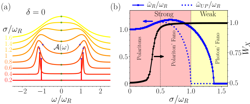
Figure 3: The evolution of the Fano resonances with disorder strength $\sigma$ for a resonant cavity mode ($\delta=0$). (a) The spectral weight $\mathcal{A}(\omega)$ at ${\sigma/\omega_{R}\in[0.2,1.6]}$ shown red to yellow, values labelled on the left. As $\sigma$ increases, the polariton peaks broaden due to interactions and become polaritons’ Fano resonances, which then merge together and give the photon’s Fano resonance. The blue and green dots show the actual locations ${\tilde{\omega}}_{UP},{\tilde{\omega}}_{LP},{\tilde{\omega}}_{c}$ of the resonances as determined by the jumps in the phase $\Delta(\omega)$. (b) The Rabi splitting $\tilde{\omega}_{R}$ or the location of the upper polariton peak in ${\mathcal{A}(\omega)}$ and ${\tilde{\omega}}_{UP}$ as a function of $\sigma$ again at ${\delta=0}$ as in (a). The emitter weight $W_{X}$ in the state at the absorption peak is also shown, see the scale on the right. A finite splitting (${\tilde{\omega}_{R}>0}$) exists even in the weak coupling regime ${\sigma/\omega_{R}\geq 1}$ Zeb (2022). Furthermore, even the strong coupling does not guarantee the hybrid excitations, ${W_{X}\simeq 1}$ coexisting with ${\tilde{\omega}_{R}\sim\omega_{R}}$ in the middle region.

IV Effect of energetic disorder on the eigenstates

IV.1 Rabi splitting and polaritons

We now focus on the optical absorption and see how the Rabi splitting $\tilde{\omega}_{R}$ observed in the absorption spectrum depends on the energetic disorder $\sigma$, and wether a finite splitting necessarily means the formation of polaritons or the strong matter-light coupling. This is an important question as the optical spectrum can exhibit a similar two-peak structure even when the underlying quantum states are entirely different, as explained below. In the absence of energetic disorder, $\mathcal{\hat{H}}_{B,1_{ex}}$ has only two polariton states given in sec. II.1, which are observed in experimental optical spectra as two sharp peaks at $\omega_{UP},\omega_{LP}$ (Eq. 5,6) with a non-zero linewidth due to homogeneous broadening $\gamma$ and cavity leakage $\kappa$ ($\kappa,\gamma\ll\omega_{R}$). However, in the presence of energetic disorder, we have a continuum of states $\ket{{\Psi}(\omega)}$ that can also produce two peaks in the absorption just like the polaritons in the above case. In the following, we first present our results of optical spectrum which pertains to the states $\ket{{\Psi}(\omega)}$. We will discuss the differences from the other case described above in sec. IV.2.

Figure 3(a) shows the evolution of the photon spectral weight $\mathcal{A}(\omega)$ with $\sigma$ for ${\sigma/\omega_{R}\in[0.2,1.6]}$ (shown red to yellow) for a resonant cavity, ${\delta=\omega_{c}-\omega_{0}=0}$. The roots of Eq. 20 are also shown as blue (${\tilde{\omega}}_{UP},{\tilde{\omega}}_{LP}$) and green (${{\tilde{\omega}}_{c}=0}$) dots to compare them with the peaks positions. At small $\sigma$, we have two sharp peaks for the upper and the lower polaritons which broaden and shift as $\sigma$ increases, and finally merge together into a single broad central peak. At ${\sigma/\omega_{R}=0.2}$, the peaks are ultra sharp and their locations agree to ${\tilde{\omega}}_{UP},{\tilde{\omega}}_{LP}$ (and the clean case $\pm\omega_{R}$, Eqs. 5,6). This can be understood by ignoring the bright states away from $\omega\simeq 0$ as they do not have significant effect on the polaritonic eigenstates formed by the coupling between $\ket{1_{P}}$ and $\ket{\mathcal{S}_{0}(0)}$. However, at higher ${\sigma}$, still in the strong coupling case, the peaks are shifted slightly outwards from ${\tilde{\omega}}_{UP},{\tilde{\omega}}_{LP}$. This can also be explained as arising from the coupling of $\ket{1_{P}}$ with the detuned bright states on either side of the ${\omega=0}$. Consider the bright states at ${\omega\gtrsim 0}$. It will push both lower and upper polaritons upwards by an amount that would depend on their detuning from the polaritons, which is ${\omega_{R}-\omega}$ for the upper polariton but ${\omega_{R}+\omega}$ for the lower polariton. So the effect on the upper polariton will be stronger. Similarly, the bright states at ${\omega\lesssim 0}$ that pull down the polaritons will affect the lower polariton more strongly, leading to a net upward shift of the upper polariton and a net downward shift of the lower polariton. The bright states within the two polaritonic states will have this effect. At ${\sigma/\omega_{R}\lesssim 1}$, the effective collective coupling of these states becomes weaker and comparible to the bright states outside this polaritons window, so all these states obtain significant photon component leading to excessively broad absorption peaks. At $\sigma/\omega_{R}\geq 1$, ${\tilde{\omega}}_{UP},{\tilde{\omega}}_{LP}$ do not exist and we are in the weak coupling regime with a single root ${\tilde{\omega}}_{c}=0$, but, as we can see, $\mathcal{A}(\omega)$ still keeps its two-peak structure at $\sigma/\omega_{R}=1,1.2$.

Thus, as $\sigma$ increases, the interactions transform the polaritons into two polariton’s Fano resonances, which are eventually replaced by a single photon Fano resonance at $\sigma/\omega_{R}\geq 1$. For clarity, we call it a polariton’s Fano resonance when the hybrid polaritonic character of the eigenstate is compromised due to Fano broadening. We can think of the polariton’s Fano resonances as arising from the interaction of polaritons (formed by cavity mode and bright states that are resonant or more strongly coupled to it) and off-resonant or less strongly coupled bright states, as illustrated in Fig. 1(c-d) and also discussed in sec. III.1.1. However, it is worth noting that this is not strictly the same as Fano resonances arising from a weak coupling between two discrete states and a continuum Fano (1961). At large enough $\sigma$, there are not enough states or coupling strength to create the strong coupling resonances, so we obtain a single photon Fano resonance in this weak coupling regime.

It is also interesting to see that at $\omega={\tilde{\omega}}_{UP},{\tilde{\omega}}_{LP},{\tilde{\omega}}_{c}$, the expression for $\mathcal{A}(\omega)$ in Eq. 30 can be simplified (as the first term in the denominator vanishes) to obtain ${\omega_{R}\mathcal{A}(\omega)=\sqrt{2/\pi^{3}}\sigma/\omega_{R}\,\exp(\omega^{2}/2\sigma^{2})}$, so that the size of the central peak is always proportional to $\sigma$. Since the spectral function is normalised, increasing $\sigma$ thus decreases the linewidth of the central peak at $\sigma/\omega_{R}>1$. This gives the correct picture in case of $\sigma/\omega_{R}\gg 1$ where the coupling becomes too weak and the cavity photon state is only slightly perturbed by the interaction with the bright continuum.

In Fig. 3(b), the Rabi splitting $\tilde{\omega}_{R}$ or the position of the upper polariton peak in $\mathcal{A}(\omega)$, and the actual location of the related resonance ${\tilde{\omega}}_{UP}$, are shown as a function of $\sigma$ again at ${\delta=0}$. We see that, as $\sigma$ increases, $\tilde{\omega}_{R}$ slightly increases at small $\sigma$ and then decreases sharply to zero at large $\sigma$ where the two peaks in Fig. 3(a) merge together. ${\tilde{\omega}}_{UP}$ also shows a similar behaviour but slightly quicker leading to an interesting situation where $\mathcal{A}(\omega)$ has two peaks with $\tilde{\omega}_{R}>0$ even in the weak coupling regime, $\sigma/\omega_{R}\geq 1$. In the strong coupling case, these peaks should exist because the first term in the denominator of Eq. 30 becomes non-monotonic Zeb (2022)) (vanishes at multiple locations) but here it is sustained because its sum with the second term still bears a bimodal structure.

Thus we find important implications for the experiments on disordered systems: the Rabi splitting, or the anticrossing in the optical absorption or transmission spectrum alone cannot guarantee the formation of polaritons or the strong coupling. Besides, strictly speaking, these two terms should not be considered synonymous in case of disordered systems as there is a wide range of $\sigma/\omega_{R}$ in the strong coupling regime where even the eigenstates containing the largest photon spectral weight are still far from truly hybrid polaritons. This will be further explained in the following section.

IV.2 Inhomogeneous vs homogeneous broadening

Let’s see how the effects of an inhomogeneous broadening or energetic disorder $\sigma$ are different from that of a homogeneous broadening or the intrinsic linewidth $\gamma$ of the emitter states. We can compare the spectrum in Fig. 3(a) to that of a system with no energetic disorder but a large homogeneous broadening, e.g., atoms in a microcavity as in Ref. Thompson et al. (1992) (see Fig. 2 there). While the spectra look similar, their physical interpretation depends on the nature of the quantum states of the system, which is different in the two cases. The homogeneous broadening of the emitter states $\gamma$ broadens the polaritonic eigenstates or polaritons around their expected energy ($\pm\omega_{R}$ at $\delta=0$) and keep their polaritonic character intact. In contrast, the inhomogeneous broadening $\sigma$ (that creates the continuum of the bright emitter states in the first place) broadens the photon spectral function only without broadening the eigenstates, making the polariton states at the absorption peaks more excitonic or emitter-like as $\sigma$ increases. That is, the polaritonic character of the eigenstates is distributed over larger number of eigenstates, making even the most polaritonic state nearly excitonic when the Fano broadening spans a large number of emitter-states in the bright continuum.

This is best illustrated by considering a specific density of continuum states and numerically evaluating the emitter weight of the most polaritonic eigenstate. For example, taking one bright state every ${\Delta\omega=0.003\omega_{R}}$, the emitter weight $W_{X}$ of the states at the absorption peaks is plotted in Fig. 3(b) [black curve] as a function of $\sigma$ at $\delta=0$. We see that $W_{X}\sim 1/2$ (polaritons) at $\sigma\lesssim 0.3$ where the Fano broadening is still smaller than the “width” $\Delta\omega$ of a single eigenstate, but quickly approaches unity around $\sigma\simeq 0.5$ where the Fano broadening distributes the photon spectral weight over many eigenstates. Thus polaritons lose their meanings and the peaks in the optical absorption simply correspond to strongly absorbing emitter states. As the figure shows, this happens at $\sigma/\omega_{R}$ as low as $0.5$ with $\tilde{\omega}_{R}\simeq\omega_{R}$, i.e., well below the threshold for the weak coupling $\sigma/\omega_{R}=1$.

This raises another question that ought to be discussed here. What does $\Delta\omega$ corresponds to in a real system? An intuitive answer to this question is that it plays the role of the intrinsic linewidth or the homogeneous broadening $\gamma$ of the emitter states (i.e., ${\Delta\omega\simeq\gamma}$). Increasing the homogeneous broadening $\gamma$ for the emitter states should extend the bright band on either side by ${\gamma/2}$ but reduce the number of such homogeneously broadened bright states in the band (${\simeq W/\gamma}$). This should enhance the polaritonic character of the states at the cost of their broadening. In the extreme case ${\gamma\to W}$, the bright band will become a homogeneously broadened bright state that would produce two homogeneously broadened polaritons as observed in Ref. Thompson et al. (1992).

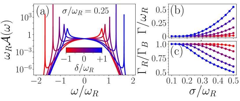
Figure 4: Fano broadening as a function of detuning $\delta$ and disorder strength $\sigma$. (a) Optical absorption at $\delta/\omega_{R}\in[-1,1]$ shown red to blue at $\sigma/\omega_{R}=0.25$. The closer a peak is to the centre of the bright band, the broader it gets. (b,c) The linewidth $\Gamma$ and the ratio of the half widths $\Gamma_{R}/\Gamma_{B}$ of the lower polariton peak as a function of $\sigma$ at the same parameters as in (a). $\Gamma$ increases almost quadratically with $\sigma$. The effect is stronger for the positive detuning where the lower polariton peak is closer to the bright band centre. The deviation of $\Gamma_{R}/\Gamma_{B}$ from unity also follows the trend of $\Gamma$.

IV.3 Fano broadening: shape and width of polaritonic peaks

Let’s focus on the Fano broadening and the lineshape asymmetry in the strong coupling regime even when the corresponding weak coupling case exhibits a symmetric Lorentzian profile. We find that the Fano broadening appears even at fairly small $\sigma$. Figure 4(a) shows the scaled spectral weight ${\omega_{R}\mathcal{A}(\omega)}$ at ${\sigma/\omega_{R}=0.25}$ and ${\delta/\omega_{R}\in[-1,+1]}$. We see that as a polariton peak gets near the bright emitter band, its linewidth increases and it transforms into a Fano resonance. This also accompanies a slight shift in the peak position compared to the clean case ${\sigma\to 0}$, Eqs. 5,6, and the actual locations of the resonance ${{\tilde{\omega}}_{UP},{\tilde{\omega}}_{LP}}$, as discussed before for ${\delta=0}$. Considering the peak corresponding to the lower polariton, Fig. 4(b,c) show its linewidth $\Gamma$ and a simple measure of the asymmetry of its lineshape, the ratio of the half linewidths of the low ($\Gamma_{R}$) and the high ($\Gamma_{B}$) energy side of the peak, as functions of $\sigma$ for the same set of $\delta$ values as in Fig. 4(a). We see that $\Gamma$ increases with $\sigma$ much more strongly at large positive detuning (bluish curves) where the lower polariton is closer to the bright emitter band and would be more matter-like even at $\sigma=0$. The lineshape asymmetry shown in Fig. 4(c), the deviation of ${\Gamma_{R}/\Gamma_{B}}$ from $1$, also shows the same trend.

We will now consider a small homogeneous broadening and treat it using the standard Green’s function formalism. To treat both homogeneous and inhomogeneous broadening of the emitter states on equal footing, new methods need to be developed, which is clearly beyond the scope of the present work.

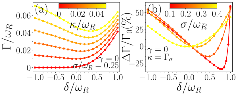
Figure 5: Total broadening as a function of disorder strength $\sigma$ and detuning $\delta$ in presence of a small homogeneous broadening $\kappa$ of the cavity state. (a) $\Gamma$ as a function of $\delta$ at $\kappa/\omega_{R}\in[0,0.05]$ shown red to yellow. $\Gamma\to\kappa$ at large negative $\delta$ while ${\Gamma\to\Gamma_{\sigma}=\Gamma(\sigma,\gamma=0=\kappa,\delta/\omega_{R}=+1)}$ at large positive $\delta$ [the blue curve in Fig. 4(b)]. (b) The percentage change in $\Gamma$ as $\delta$ changes from zero, at $\sigma/\omega_{R}\in[0.1,0.4]$, $\kappa=\Gamma_{\sigma}$, $\gamma=0$.

V Optical absorption in the presence of losses

So far, we have not considered the losses, a finite cavity leakage and non-radiative emitter decay that amount to homogeneous broadening of the bare cavity and emitter states. To see the effect of these losses on the spectral function $\mathcal{A}(\omega)$ or optical absorption, we need the photon Green’s function $G(\omega)$ as ${\mathcal{A}(\omega)=-\Im G(\omega)}$, which will now be used instead of Eq. 30. Here $\Im$ stands for the imaginary part. Due to the absence of the coupling between the emitters or their bright states, $G(\omega)$ can be easily calculated from the resolvent of $\mathcal{\hat{H}}_{B,1_{ex}}$ (Appendix. VIII.2), to obtain

$$G(\omega) =\left[\omega-\omega_{c}+i\kappa-\Sigma(\omega+i\gamma)\right]^{-1},$$ (31)

$$\Sigma(z) =\omega_{R}^{2}\int d\omega^{\prime}\frac{P(\omega^{\prime})}{z-\omega^{\prime}},$$ (32)

where $\Sigma$ is the self energy and $\kappa,\gamma$ are cavity leakage and non-radiative emitter relaxation rates. Computing the self energy $\Sigma(z)$ for the Gaussian $P(\omega)$ readily gives

$$\Sigma(z) =\pi\omega_{R}^{2}P(z)\left[\operatorname{erfi}\left(\frac{z}{\sqrt{2}\sigma}\right)-i\right],$$ (33)

which can now be used with Eq. 31 to explore the optical absorption including the losses.

V.1 Lineshape and linewidth

Let’s now include the effect of cavity and emitter losses on the total broadening of absorption peaks. In systems where $\kappa\gg\gamma$, e.g., organic microcavities Ćwik et al. (2016); Dimitrov et al. (2016), we can ignore $\gamma$ to understand how $\kappa$ changes the picture discussed so far. Figure 5(a) shows $\Gamma$ as a function of $\delta$ at $\sigma/\omega_{R}=0.25$, $\gamma=0$ and $\kappa/\omega_{R}\in[0,0.05]$. We see that at large negative detuning, $|\delta|\gg\sigma$, where the polariton is away from the band and Fano broadening can be ignored, the effect of $\kappa$ is the strongest due to larger photon fraction. As $\delta$ increases to zero and positive values, the effect of $\kappa$ decreases but that of $\sigma$ increases. This leads to an interesting situation where $\Gamma$ develops a minimum at an optimum $\delta$. The minimum gets deeper and more prominent if $\Gamma$ at extreme $\delta$ values is large and of similar size. Noting that at ${\delta/\omega_{R}=-1}$, ${\Gamma\sim\kappa}$ and at ${\delta/\omega_{R}=+1}$, ${\Gamma\sim\Gamma_{\sigma}\equiv\Gamma(\sigma,\delta/\omega_{R}=+1,\kappa=0=\gamma)}$ [blue curve in Fig. 4(b)], the optimum $\kappa$ to observe such a minimum is ${\kappa=\Gamma_{\sigma}}$. This is shown in Fig. 5(b) for ${\sigma/\omega_{R}\in[0.1,0.4]}$ where percentage change in $\Gamma$, ${\Delta\Gamma/\Gamma_{0}=(\Gamma-\Gamma_{0})/\Gamma_{0}}$ is shown as $\delta$ deviates from the resonance, ${\delta=0}$, where ${\Gamma=\Gamma_{0}}$, which is used as a reference. We see that the smaller the $\sigma$, the larger the percentage change in $\Gamma$, and the larger the optimum $\delta$. It should be observable in typical organic microcavities where ${\kappa\sim 0.05eV}$ Dimitrov et al. (2016), ${2\omega_{R}\sim 1eV}$ Tropf and Gather (2018), and ${\sigma\sim\sqrt{2}\times 0.1eV}$ Bässler (1981); Bässler et al. (1982); Zeb (2021) so $\sigma/\omega_{R}\sim 0.28$, which gives the minimum at $\delta\sim 0$.

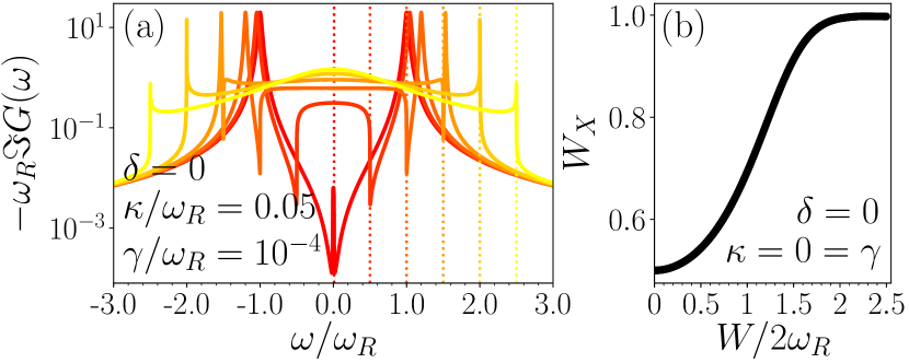
Figure 6: Evolution of the Fano resonance with the bandwidth for a flat energy distribution that leads to a flat interaction $V(\omega)$. (a) Photon spectral weight $-\omega_{R}\Im G(\omega)$ at ${\sigma/\omega_{R}=0.01,0.5-2.5}$ (indicated by vertical lines). (b) Emitter weight $W_{X}$ as a function of the bandwidth $W$.

V.2 Dependence on the energy distribution

If the emitter transition energies are distributed more evenly, the distribution function is flatter in the middle and falls more sharply at the edges. We would expect it should result in a sharper transition between polaritons and their Fano resonances as the polariton energy starts overlapping the bright states band. Taking the extreme case of a flat distribution, ${P(\omega)=1/W,-W/2\leq\omega\leq W/2,0}$ otherwise, we find that the transition actually becomes more gradual. This is because in this case all bright states would couple equally strongly to the cavity mode (as ${V(\omega)=\omega_{R}/\sqrt{W}=constant}$) and increasing $W$ would push the polaritons away from the band edges at small to intermediate $W$. In this case, Eq. 32 gives

$$\Sigma(z) =\frac{\omega_{R}^{2}}{W}\ln\left(\frac{z+W/2}{z-W/2}\right).$$ (34)

Figure 6(a) shows the scaled spectral weight $-\omega_{R}\Im G(\omega)$ for the flat distribution (Eq. 31 with Eq. 34) at ${\delta=0}$, ${\kappa/\omega_{R}=0.05}$, ${\gamma/\omega_{R}=10^{-4}}$ ($\kappa,\gamma$ typical of organic microcavities, Ćwik et al. (2016); Dimitrov et al. (2016)) and ${W/2\omega_{R}=0.01,0.5-2.5}$ in increments of $0.5$, marked with dotted vertical lines. We see that it has a feature resembling Fano lineshape with a dip but note the logscale, these structures differ from the weak coupling Fano profile indeed. At $W<2\omega_{R}$, the peaks resemble isolated polaritonic states. Despite the change in lineshape at $W\geq 2\omega_{R}$, they still remain quite hybrid for a while. $W_{X}$ for the lower polariton state at the peak position at ${\delta=0=\kappa=\gamma}$ is shown in Fig. 6(b). We see that $W_{X}$ increases from ${1/2}$ to $1$ over a wider $\sigma$ range: $W_{X}\simeq 0.7$ only at $W/2\omega_{R}=1$ and it increases to $0.9$ around $W/2\omega_{R}=1.5$. Compare this to the gaussian energy distribution, where $W_{X}$ jumps to $\sim 0.95$ around $\sigma/\omega_{R}=0.5$ only. This sluggish increase in the emitter weight for the flat distribution can be understood as a result of poor correspondence of $\omega_{R}$ itself to the Rabi splitting $\tilde{\omega}_{R}$, because the bright states at the band edge couple equally strongly to the cavity mode and their effective detuning from it shifts the polariton energy more significantly. Another difference from the gaussian distribution case is that the photon Fano resonance appears before the polaritons’ Fano resonances disappear. So the notion of the Rabi splitting $\tilde{\omega}_{R}$ also becomes relatively vague at $W/2\omega_{R}\gtrsim 2$ in this case. Interestingly, however, for polaritonic peaks, a significant linewidth narrowing occurs at $W\gtrsim 2\omega_{R}$, as can be seen in Fig. 6(a).

VI Summary and conclusions

We solve the disordered TC model by identifying and decoupling the exact bright and dark sectors of the emitters’ Hilbert space. Explicit expressions for the bright and the dark states are presented, allowing the exact numerical diagonalisation for arbitrarily large systems. For the emitter states forming a continuum in the thermodynamic limit, we obtain Fano’s model whose solution has already been around for a long time. The Fano resonances in the optical absorption and inelastic electron scattering spectra are presented both in the strong and the weak coupling regimes, where they correspond to polaritons or their Fano resonances and photon’s Fano resonance, respectively. We find that the hybrid light-matter character of the excitations could be lost due to strong energetic disorder while the optical spectra still showing the Rabi splitting and anticrossing. We also explore the effect of cavity and emitter losses on the linewidth and lineshape by calculating the photon Green’s function. We find that the polariton’s linewidth should exhibit a minimum as a function of the detuning when the cavity losses are comparable to the maximum Fano broadening.

VII Outlook

We studied the model in the rotating wave approximation that ignores the counter rotating terms in the light-matter interaction. These terms introduce coupling within a given parity subspace ($N_{ex}$ even or odd) which are usually ignored below the “ultra-strong” coupling regime ($\omega_{R}\gtrsim 0.3\omega_{0}$) due to a large energetic difference ($\simeq 2\omega_{0}$) between the coupled states. However, energetic disorder would reduce this energetic difference and, at large energetic disorder, the highest end of the bright band or the upper polariton in ${N_{ex}=1}$ subspace would come close enough to (or overlap with) the lowest end of the bright band or the lower polariton in ${N_{ex}=3}$ subspace such that their interaction cannot be ignored any longer. Similarly, the effects of an interaction that does not respect the excitation number parity (coupling to a bath, for instance) on the eigenstates of the system, would be enhanced even further as it would only require to reduce the gap ($\simeq\omega_{0}$) between the states of adjacent excitation spaces (e.g., ${N_{ex}=1}$ and ${N_{ex}=2}$). Investigation of such effects of the energetic disorder can be carried out in a future study. Considering a weak coupling between the bright and dark spaces due to dipole-dipole interaction and application of the two spaces in other systems, e.g., those described by the Anderson impurity model, and exploring the effects of Fano broadening on highly excited states such as polariton condensate and lasing would also be interesting future works.

VIII Appendix

VIII.1 Calculations of $\ket{{\Phi}(\omega)}$ and $\ket{{\Psi}(\omega)}$

VIII.1.1 Eigenstates and energies outside the bright band

Assuming that $\ket{{\Phi}(\omega)}$ represents a discrete eigenstate of $\mathcal{\hat{H}}_{B,1_{ex}}$ at energy $\omega$ outside the bright continuum, it can be written as a superposition of the form

$$\ket{{\Phi}(\omega)}=\ket{1_{P}}+\int{B(\omega,\omega^{\prime})\ket{\mathcal{S}_{0}(\omega^{\prime})}d\omega^{\prime}},$$ (35)

where the integration is over the bright band. By substituting $\ket{{\Phi}(\omega)}$ into the eigenvalue equation ${\mathcal{\hat{H}}_{B,1_{ex}}\ket{{\Phi}(\omega)}=\omega\ket{{\Phi}(\omega)}}$, projecting it onto $\ket{1_{P}}$ and $\ket{\mathcal{S}_{0}(\omega^{\prime\prime})}$ in turns, and using the orthonormality of the basis states, ${\braket{1_{P}}{1_{P}}=1}$, ${\braket{\mathcal{S}_{0}(\omega^{\prime})}{\mathcal{S}_{0}(\omega^{\prime\prime})}=\delta(\omega^{\prime}-\omega^{\prime\prime})}$, and ${\braket{1_{P}}{\mathcal{S}_{0}(\omega^{\prime})}=0}$, we obtain the following two coupled equations,

$$\omega_{c}+\int V(\omega^{\prime})B(\omega,\omega^{\prime})d\omega^{\prime} =\omega,$$ (36)

$$V(\omega^{\prime})+\omega^{\prime}B(\omega,\omega^{\prime}) =\omega B(\omega,\omega^{\prime}),$$ (37)

which can be easily solved as ${\omega\neq\omega^{\prime}}$ to get

$$B(\omega,\omega^{\prime}) =\frac{V(\omega^{\prime})}{\omega-\omega^{\prime}},$$ (38)

$$\omega =\omega_{c}+\int{d\omega^{\prime}\frac{V(\omega^{\prime})^{2}}{\omega-\omega^{\prime}}},$$ (39)

where the last equation contains $\omega$ in the integral on the right side as well and can be solved for $\omega$ numerically when $V(\omega)$ is specified. Substituting the above expression for $B(\omega,\omega^{\prime})$ into the Eq. 35 above gives Eq. 19 in the main text, while Eq. 39 is rewritten as Eqs. 20,21 there.

VIII.1.2 Eigenstates inside the bright band

Assuming $\ket{{\Psi}(\omega)}$ is an eigenstate of $\mathcal{\hat{H}}_{B,1_{ex}}$ at an energy within the bright continuum, we can again write it as a superposition,

$$\ket{{\Psi}(\omega)}=\alpha(\omega)\ket{1_{P}}+\int{\beta(\omega,\omega^{\prime})\ket{\mathcal{S}_{0}(\omega^{\prime})}d\omega^{\prime}},$$ (40)

where the coefficients $\alpha,\beta$ can be written in terms of ${\Delta(\omega),F(\omega)}$ given in the main text as (see Ref. Fano (1961) for detailed derivation),

$$\alpha(\omega) =\sin\Delta(\omega)/\pi V(\omega),$$ (41)

$$\beta(\omega,\omega^{\prime}) =\alpha(\omega)\frac{V(\omega^{\prime})}{\omega-\omega^{\prime}}-\cos\Delta(\omega)\delta(\omega-\omega^{\prime}),$$ (42)

Here, $\delta$ is the Dirac delta function. Substituting these back, we obtain,

$$\ket{{\Psi}(\omega)}=\frac{\sin\Delta(\omega)}{\pi V(\omega)}\left(\ket{1_{P}}+\int{\frac{V(\omega^{\prime})}{\omega-\omega^{\prime}}\ket{\mathcal{S}_{0}(\omega^{\prime})}d\omega^{\prime}}\right)\\ -\cos\Delta(\omega)\ket{\mathcal{S}_{0}(\omega)},$$ (43)

which along with $\ket{{\Phi}(\omega)}$ in Eq. 19 at $\omega$ inside the bright band (where it does not represent an eigenstate in general), gives Eq. 22.

VIII.2 Calculation of $G(\omega)$

The photon Green’s function $G(\omega)$ can be obtained Mazhorin et al. (2022) from the resolvent $\mathcal{R}(\omega)$ of $\mathcal{\hat{H}}_{B,1_{ex}}$, as follows. We start from the discrete version $\mathcal{\hat{H}}_{B}$ in Eq. 13. In the single excitation space, it can be written in the matrix form as,

$$\mathcal{H}_{B} =\begin{pmatrix}\omega_{c}&G_{1,K_{1}}&G_{2,K_{2}}&...&G_{N,K_{N}}\\ G_{1,K_{1}}&\omega_{1}&0&...&0\\ G_{2,K_{2}}&0&\omega_{2}&...&0\\ ...&...&...&...&...\\ G_{N,K_{N}}&0&0&...&\omega_{N}\end{pmatrix}.$$

Its resolvent $\mathcal{R}(\omega)$ is given as $\mathcal{R}(\omega)=(I\omega-\mathcal{H}_{B})^{-1}$, where $I$ is identity. It can be computed by partitioning $I\omega-\mathcal{H}_{B}$ in four blocks as,

$$I\omega-\mathcal{H}_{B} =\begin{pmatrix}A_{1\times 1}&B_{1\times N}\\ C_{N\times 1}&D_{N\times N}\end{pmatrix},$$

to take the inverse, where the subscripts with the matrix elements show the dimensions of each block. The matrix element of $\mathcal{R}(\omega)$ corresponding to the cavity state is the photon Green’s function $G(\omega)$, given by Lu and Shiou (2002) ${G(\omega)=(A-BD^{-1}C)^{-1}}$. Since $D$ is diagonal, its inverse can be written directly, and we obtain

$$G(\omega) =\left[\omega-\omega_{c}+i\kappa-\Sigma(\omega)\right]^{-1},$$ (44)

$$\Sigma(\omega) =\sum_{n=1}^{N}\frac{G_{n,K_{n}}^{2}}{\omega-\omega_{n}+i\gamma},$$ (45)

where we have added the imaginary components $\kappa,\gamma$ to $\omega_{c},\omega_{n}$ to include a finite cavity leakage and non-radiative emitter relaxation. Considering the continuous limit leads to Eq. 31.

References

- Walther et al. (2006) H. Walther, B. T. H. Varcoe, B.-G. Englert, and T. Becker, Reports on Progress in Physics 69, 1325 (2006).
- Mivehvar et al. (2021) F. Mivehvar, F. Piazza, T. Donner, and H. Ritsch, Advances in Physics 70, 1 (2021), https://doi.org/10.1080/00018732.2021.1969727 .
- Lidzey et al. (1998) D. G. Lidzey, D. Bradley, M. Skolnick, T. Virgili, S. Walker, and D. Whittaker, Nature 395, 53 (1998).
- Keeling and Kéna-Cohen (2020) J. Keeling and S. Kéna-Cohen, Ann. Rev. Phys. Chem. 71 (2020), 10.1146/annurev-physchem-010920-102509.
- Kiraz et al. (2003) A. Kiraz, C. Reese, B. Gayral, L. Zhang, W. V. Schoenfeld, B. D. Gerardot, P. M. Petroff, E. L. Hu, and A. Imamoglu, Journal of Optics B: Quantum and Semiclassical Optics 5, 129 (2003).
- Stockklauser et al. (2017) A. Stockklauser, P. Scarlino, J. V. Koski, S. Gasparinetti, C. K. Andersen, C. Reichl, W. Wegscheider, T. Ihn, K. Ensslin, and A. Wallraff, Phys. Rev. X 7, 011030 (2017).
- Najer et al. (2019) D. Najer, I. Söllner, P. Sekatski, V. Dolique, M. C. Löbl, D. Riedel, R. Schott, S. Starosielec, S. R. Valentin, A. D. Wieck, N. Sangouard, A. Ludwig, and R. J. Warburton, Nature 575, 622 (2019).
- Colombe et al. (2007) Y. Colombe, T. Steinmetz, G. Dubois, F. Linke, D. Hunger, and J. Reichel, Nature 450, 272 (2007).
- Brennecke et al. (2007) F. Brennecke, T. Donner, S. Ritter, T. Bourdel, M. Köhl, and T. Esslinger, Nature 450, 268 (2007).
- Vaidya et al. (2018) V. D. Vaidya, Y. Guo, R. M. Kroeze, K. E. Ballantine, A. J. Kollár, J. Keeling, and B. L. Lev, Phys. Rev. X 8, 011002 (2018).
- Guo et al. (2019) Y. Guo, R. M. Kroeze, V. D. Vaidya, J. Keeling, and B. L. Lev, Phys. Rev. Lett. 122, 193601 (2019).
- Periwal et al. (2021) A. Periwal, E. S. Cooper, P. Kunkel, J. F. Wienand, E. J. Davis, and M. Schleier-Smith, Nature 600, 630 (2021).
- Georges et al. (2018) C. Georges, J. G. Cosme, L. Mathey, and A. Hemmerich, Phys. Rev. Lett. 121, 220405 (2018).
- Clark et al. (2020) L. W. Clark, N. Schine, C. Baum, N. Jia, and J. Simon, Nature 582, 41 (2020).
- Dovzhenko et al. (2018) D. S. Dovzhenko, S. V. Ryabchuk, Y. P. Rakovich, and I. R. Nabiev, Nanoscale 10, 3589 (2018).
- Basov et al. (2021) D. N. Basov, A. Asenjo-Garcia, P. J. Schuck, X. Zhu, and A. Rubio, Nanophotonics 10, 549 (2021).
- Kasprzak et al. (2006) J. Kasprzak, M. Richard, S. Kundermann, A. Baas, P. Jeambrun, J. M. J. Keeling, F. M. Marchetti, M. H. Szymańska, R. André, J. L. Staehli, V. Savona, P. B. Littlewood, B. Deveaud, and L. S. Dang, Nature 443, 409 (2006).
- Houck et al. (2012) A. A. Houck, H. E. Türeci, and J. Koch, Nature Physics 8, 292 (2012).
- Sanvitto and Kéna-Cohen (2016) D. Sanvitto and S. Kéna-Cohen, Nat. Mater. 15, 1061 (2016).
- Kravtsov et al. (2020) V. Kravtsov, E. Khestanova, F. A. Benimetskiy, T. Ivanova, A. K. Samusev, I. S. Sinev, D. Pidgayko, A. M. Mozharov, I. S. Mukhin, M. S. Lozhkin, Y. V. Kapitonov, A. S. Brichkin, V. D. Kulakovskii, I. A. Shelykh, A. I. Tartakovskii, P. M. Walker, M. S. Skolnick, D. N. Krizhanovskii, and I. V. Iorsh, Light: Science & Applications 9, 56 (2020).
- Moxley et al. (2021) F. I. Moxley, E. O. Ilo-Okeke, S. Mudaliar, and T. Byrnes, Emergent Materials 4, 971 (2021).
- Tavis and Cummings (1968) M. Tavis and F. W. Cummings, Phys. Rev. 170, 379 (1968).
- Ribeiro et al. (2018) R. F. Ribeiro, L. A. Martínez-Martínez, M. Du, J. Campos-Gonzalez-Angulo, and J. Yuen-Zhou, Chem. Sci. 9, 6325 (2018).
- Zeb (2021) M. A. Zeb, “Supplemental material,” (2021), see supplemental material for technical details.
- Ćwik et al. (2016) J. A. Ćwik, P. Kirton, S. De Liberato, and J. Keeling, Phys. Rev. A 93, 033840 (2016).
- Botzung et al. (2020) T. Botzung, D. Hagenmüller, S. Schütz, J. Dubail, G. Pupillo, and J. Schachenmayer, Phys. Rev. B 102, 144202 (2020).
- Du and Yuen-Zhou (2022) M. Du and J. Yuen-Zhou, Phys. Rev. Lett. 128, 096001 (2022).
- Blaha et al. (2022) M. Blaha, A. Johnson, A. Rauschenbeutel, and J. Volz, Phys. Rev. A 105, 013719 (2022).
- Huang et al. (2019) J. Huang, A. J. Traverso, G. Yang, and M. H. Mikkelsen, ACS Photonics 6, 838 (2019).
- Mazhorin et al. (2022) G. S. Mazhorin, I. N. Moskalenko, I. S. Besedin, D. S. Shapiro, S. V. Remizov, W. V. Pogosov, D. O. Moskalev, A. A. Pishchimova, A. A. Dobronosova, I. A. Rodionov, and A. V. Ustinov, Phys. Rev. A 105, 033519 (2022).
- Bässler (1981) H. Bässler, physica status solidi (b) 107, 9 (1981), https://onlinelibrary.wiley.com/doi/pdf/10.1002/pssb.2221070102 .
- Bässler et al. (1982) H. Bässler, G. Schönherr, M. Abkowitz, and D. M. Pai, Phys. Rev. B 26, 3105 (1982).
- (33) The factor of for independent HOMO and LUMO distributions.
- Tropf and Gather (2018) L. Tropf and M. C. Gather, Advanced Optical Materials 6, 1800203 (2018), https://onlinelibrary.wiley.com/doi/pdf/10.1002/adom.201800203 .
- Kéna-Cohen and Forrest (2010) S. Kéna-Cohen and S. Forrest, Nat. Phot. 4, 371 (2010).
- Plumhof et al. (2013) J. D. Plumhof, T. Stöferle, L. Mai, U. Scherf, and R. F. Mahrt, Nat. Mater. 13, 247 (2013).
- Feist and Garcia-Vidal (2015) J. Feist and F. J. Garcia-Vidal, Phys. Rev. Lett. 114, 196402 (2015).
- Hagenmüller et al. (2017) D. Hagenmüller, J. Schachenmayer, S. Schütz, C. Genes, and G. Pupillo, Phys. Rev. Lett. 119, 223601 (2017).
- Schäfer et al. (2019) C. Schäfer, M. Ruggenthaler, H. Appel, and A. Rubio, Proc. Natl. Acad. Sci. U. S. A. 116, 4883 (2019).
- Zeb et al. (2020) M. A. Zeb, P. G. Kirton, and J. Keeling, “Incoherent charge transport in an organic polariton condensate,” (2020), arXiv:2004.09790 [cond-mat.quant-gas] .
- Thomas et al. (2019) A. Thomas, L. Lethuillier-Karl, K. Nagarajan, R. M. A. Vergauwe, J. George, T. Chervy, A. Shalabney, E. Devaux, C. Genet, J. Moran, and T. W. Ebbesen, Science 363, 615 (2019).
- Herrera and Spano (2016) F. Herrera and F. C. Spano, Phys. Rev. Lett. 116, 238301 (2016).
- Galego et al. (2016) J. Galego, F. J. Garcia-Vidal, and J. Feist, Nat. Commun. 7, 13841 (2016).
- Galego et al. (2017) J. Galego, F. J. Garcia-Vidal, and J. Feist, Phys. Rev. Lett. 119, 136001 (2017).
- Martínez-Martínez et al. (2018) L. A. Martínez-Martínez, R. F. Ribeiro, J. Campos-González-Angulo, and J. Yuen-Zhou, ACS Photonics 5, 167 (2018).
- Ebbesen (2016) T. W. Ebbesen, Acc. Chem. Res 49, 2403 (2016).
- Feist et al. (2017) J. Feist, J. Galego, and F. J. Garcia-Vidal, ACS Photonics 5, 205 (2017).
- Kéna-Cohen and Yuen-Zhou (2019) S. Kéna-Cohen and J. Yuen-Zhou, ACS Central Science 5, 386 (2019).
- Agranovich et al. (2002) V. Agranovich, M. Litinskaia, and D. Lidzey, physica status solidi (b) 234, 130 (2002).
- Agranovich et al. (2003) V. M. Agranovich, M. Litinskaia, and D. G. Lidzey, Phys. Rev. B 67, 085311 (2003).
- Gonzalez-Ballestero et al. (2016) C. Gonzalez-Ballestero, J. Feist, E. Gonzalo Badía, E. Moreno, and F. J. Garcia-Vidal, Phys. Rev. Lett. 117, 156402 (2016).
- Hu et al. (2018) Z. Hu, G. S. Engel, F. H. Alharbi, and S. Kais, The Journal of Chemical Physics 148, 064304 (2018), https://doi.org/10.1063/1.5009903 .
- Pandya et al. (2022) R. Pandya, A. Ashoka, K. Georgiou, J. Sung, R. Jayaprakash, S. Renken, L. Gai, Z. Shen, A. Rao, and A. J. Musser, Advanced Science 9, 2105569 (2022), https://onlinelibrary.wiley.com/doi/pdf/10.1002/advs.202105569 .
- del Pino et al. (2018) J. del Pino, F. A. Y. N. Schröder, A. W. Chin, J. Feist, and F. J. Garcia-Vidal, Phys. Rev. Lett. 121, 227401 (2018).
- Groenhof et al. (2019) G. Groenhof, C. Climent, J. Feist, D. Morozov, and J. J. Toppari, The Journal of Physical Chemistry Letters 10, 5476 (2019), pMID: 31453696, https://doi.org/10.1021/acs.jpclett.9b02192 .
- Sommer et al. (2021) C. Sommer, M. Reitz, F. Mineo, and C. Genes, Phys. Rev. Research 3, 033141 (2021).
- Eizner et al. (2019) E. Eizner, L. A. Martínez-Martínez, J. Yuen-Zhou, and S. Kéna-Cohen, Science Advances 5 (2019), 10.1126/sciadv.aax4482, https://advances.sciencemag.org/content/5/12/eaax4482.full.pdf .
- Polak et al. (2020) D. Polak, R. Jayaprakash, T. P. Lyons, L. A. Martínez-Martínez, A. Leventis, K. J. Fallon, H. Coulthard, D. G. Bossanyi, K. Georgiou, A. J. Petty, II, J. Anthony, H. Bronstein, J. Yuen-Zhou, A. I. Tartakovskii, J. Clark, and A. J. Musser, Chem. Sci. 11, 343 (2020).
- Yu et al. (2021) Y. Yu, S. Mallick, M. Wang, and K. Börjesson, Nature Communications 12, 3255 (2021).
- Mewes et al. (2020) L. Mewes, M. Wang, R. A. Ingle, K. Börjesson, and M. Chergui, Communications Physics 3, 157 (2020).
- Wersäll et al. (2019) M. Wersäll, B. Munkhbat, D. G. Baranov, F. Herrera, J. Cao, T. J. Antosiewicz, and T. Shegai, ACS Photonics 6, 2570 (2019), https://doi.org/10.1021/acsphotonics.9b01079 .
- Xiang et al. (2019) B. Xiang, R. F. Ribeiro, L. Chen, J. Wang, M. Du, J. Yuen-Zhou, and W. Xiong, The Journal of Physical Chemistry A 123, 5918 (2019), pMID: 31268708, https://doi.org/10.1021/acs.jpca.9b04601 .
- Thompson et al. (1992) R. J. Thompson, G. Rempe, and H. J. Kimble, Phys. Rev. Lett. 68, 1132 (1992).
- Herrera and Spano (2017) F. Herrera and F. C. Spano, Phys. Rev. A 95, 053867 (2017).
- Zhang and Zhang (2021) Q. Zhang and K. Zhang, Journal of Physics B: Atomic, Molecular and Optical Physics 54, 145101 (2021).
- Dong et al. (2022) Z. Dong, G. Zhang, A.-G. Wu, and R.-B. Wu, IEEE Transactions on Automatic Control , 1 (2022).
- Gera and Sebastian (2022) T. Gera and K. L. Sebastian, The Journal of Chemical Physics 156, 194304 (2022), https://doi.org/10.1063/5.0086027 .
- Fano (1961) U. Fano, Phys. Rev. 124, 1866 (1961).
- Miroshnichenko et al. (2010) A. E. Miroshnichenko, S. Flach, and Y. S. Kivshar, Rev. Mod. Phys. 82, 2257 (2010).
- Kamenetskii et al. (2018) E. Kamenetskii, A. Sadreev, and A. Miroshnichenko, eds., Fano Resonances in Optics and Microwaves (Springer, Cham, 2018).
- Cao et al. (2020) G. Cao, S. Dong, L.-M. Zhou, Q. Zhang, Y. Deng, C. Wang, H. Zhang, Y. Chen, C.-W. Qiu, and X. Liu, Advanced Optical Materials 8, 1902153 (2020), https://onlinelibrary.wiley.com/doi/pdf/10.1002/adom.201902153 .
- Zeb (2022) M. A. Zeb, “Fano resonance in the strong coupling regime,” (2022), submitted.
- Limonov (2021) M. F. Limonov, Adv. Opt. Photon. 13, 703 (2021).
- Nozaki et al. (2013) K. Nozaki, A. Shinya, S. Matsuo, T. Sato, E. Kuramochi, and M. Notomi, Opt. Express 21, 11877 (2013).
- Stern et al. (2014) L. Stern, M. Grajower, and U. Levy, Nature Communications 5, 4865 (2014).
- Zhang et al. (2006) W. Zhang, A. O. Govorov, and G. W. Bryant, Phys. Rev. Lett. 97, 146804 (2006).
- Zhang et al. (2008) S. Zhang, D. A. Genov, Y. Wang, M. Liu, and X. Zhang, Phys. Rev. Lett. 101, 047401 (2008).
- Tang et al. (2010) T.-T. Tang, Y. Zhang, C.-H. Park, B. Geng, C. Girit, Z. Hao, M. C. Martin, A. Zettl, M. F. Crommie, S. G. Louie, Y. R. Shen, and F. Wang, Nature Nanotechnology 5, 32 (2010).
- Ott et al. (2013) C. Ott, A. Kaldun, P. Raith, K. Meyer, M. Laux, J. Evers, C. H. Keitel, C. H. Greene, and T. Pfeifer, Science 340, 716 (2013), https://www.science.org/doi/pdf/10.1126/science.1234407 .
- Luo et al. (2004) H. G. Luo, T. Xiang, X. Q. Wang, Z. B. Su, and L. Yu, Phys. Rev. Lett. 92, 256602 (2004).
- Zielinski et al. (2015) A. Zielinski, V. P. Majety, S. Nagele, R. Pazourek, J. Burgdörfer, and A. Scrinzi, Phys. Rev. Lett. 115, 243001 (2015).
- Wang et al. (2017) Y. Wang, L. Liao, T. Hu, S. Luo, L. Wu, J. Wang, Z. Zhang, W. Xie, L. Sun, A. V. Kavokin, X. Shen, and Z. Chen, Phys. Rev. Lett. 118, 063602 (2017).
- Limonov et al. (2017) M. F. Limonov, M. V. Rybin, A. N. Poddubny, and Y. S. Kivshar, Nature Photonics 11, 543 (2017).
- Poddubny et al. (2012) A. N. Poddubny, M. V. Rybin, M. F. Limonov, and Y. S. Kivshar, Nature Communications 3, 914 (2012).
- Silevitch et al. (2019) D. M. Silevitch, C. Tang, G. Aeppli, and T. F. Rosenbaum, Nature Communications 10, 4001 (2019).
- Scully and Zubairy (1997) M. O. Scully and M. S. Zubairy, Quantum Optics (Cambridge University Press, 1997).
- Zeb and Masood (2021) M. A. Zeb and S. Masood, “Spin-orbit coupling in organic microcavities: lower polariton splitting, triplet polaritons and disorder induced dark states relaxation,” (2021), preprint, 2104.07016v2 .
- Dimitrov et al. (2016) S. D. Dimitrov, B. C. Schroeder, C. B. Nielsen, H. Bronstein, Z. Fei, I. McCulloch, M. Heeney, and J. R. Durrant, Polymers 8 (2016), 10.3390/polym8010014.
- Lu and Shiou (2002) T.-T. Lu and S.-H. Shiou, Computers Mathematics with Applications 43, 119 (2002).