Local Intrinsic Dimensionality Measures for Graphs, with Applications to Graph Embeddings

Abstract

The notion of local intrinsic dimensionality (LID) is an important advancement in data dimensionality analysis, with applications in data mining, machine learning and similarity search problems. Existing distance-based LID estimators were designed for tabular datasets encompassing data points represented as vectors in a Euclidean space. After discussing their limitations for graph-structured data considering graph embeddings and graph distances, we propose NC-LID, a novel LID-related measure for quantifying the discriminatory power of the shortest-path distance with respect to natural communities of nodes as their intrinsic localities. It is shown how this measure can be used to design LID-aware graph embedding algorithms by formulating two LID-elastic variants of node2vec with personalized hyperparameters that are adjusted according to NC-LID values. Our empirical analysis of NC-LID on a large number of real-world graphs shows that this measure is able to point to nodes with high link reconstruction errors in node2vec embeddings better than node centrality metrics. The experimental evaluation also shows that the proposed LID-elastic node2vec extensions improve node2vec by better preserving graph structure in generated embeddings.

1 Introduction

The intrinsic dimensionality (ID) of a dataset is the minimal number of features that are needed to form a good representation of data in a lower-dimensional space without a large information loss. Estimation of ID is highly relevant when performing dimensionality reduction in various machine learning (ML) and data mining (DM) tasks. Namely, machine learning models can be trained on lower-dimensional data representations in order to achieve a higher level of generalizability by alleviating negative impacts of high dimensionality (e.g., negative phenomena associated with the curse of dimensionality). Due to a smaller number of features, such models are additionally more comprehensible, while their training, tuning and validation is more time efficient.

The notion of local intrinsic dimensionality (LID) has been developed in recent years motivated by the fact that the ID may vary across a dataset. The main idea of LID is to focus the estimation of ID to a data space surrounding a data point. In a seminal paper, Houle [2] defined the LID considering the distribution of distances to a reference data point. Intuitively, the LID of the reference data point expresses the degree of difficulty to separate its nearest neighbors from the rest of the dataset. Houle showed that for continuous distance distributions with differentiable cumulative density functions the LID and the indiscriminability of the corresponding distance function are actually equivalent.

Inspired by the works of Houle and collaborators [2, 3], in [1] we proposed an approach for formulating LID-related measures for nodes in graphs and complex networks. By using the proposed approach we defined one concrete LID measure called NC-LID that is based on natural or local communities [4] as intrinsic subgraph localities. In [1] we also designed two LID-elastic node2vec [5] extensions based on NC-LID measure. This works extends [1] in the following ways:

1. The empirical evalution of NC-LID and LID-elastic node2vec extensions is expanded from 10 to 18 real-world networks (15 of them being large-scale). The obtained results confirm the initial findings from [1] that (1) NC-LID significantly correlates to link reconstruction errors when reconstructing input graphs from node2vec embeddings, and (2) LID-elastic node2vec extensions outperform node2vec by providing graph embeddings that better preserve the structure of the input graphs.

2. We empirically compare NC-LID to various node centrality metrics quantifying structural importance of nodes in complex networks regarding their ability to identify nodes with high link reconstruction errors in node2vec embeddings. The results of this analysis show that NC-LID has consistent and stronger correlations to link reconstruction errors than existing node centrality measures. This finding implies that our measure is a better choice for designing “elastic” graph embedding algorithms in which hyper-parameters are adjusted according to structural measures associated to nodes.

Additionally, subsequent research by Knežević et al. [6] showed that our NC-LID based node2vec extensions outperform node2vec when utilizing generated embeddings in a concrete ML/DM application (i.e., node clustering). The implementation of NC-LID and NC-LID based node2vec extensions together with evaluation procedures and datasets used in this paper are contained in the open-source GRASPE library.

The rest of the paper is structured as follows. After presenting relevant research works in Section 2, the motivation for this work and its main contributions are outlined in Section 3. The NC-LID measure is discussed in Section 4, while the LID-elastic node2vec extensions based on NC-LID are explained in Section 5. The experimental evaluation of NC-LID and NC-LID based node2vec extensions are presented in Section 6. The last section concludes the paper and discusses possible directions for future research.

2 Related Work

2.1 Local Intrinsic Dimensionality

The theoretical foundation of LID was set by Houle who formally defined it [2] and then explored its mathematical properties in a series of papers [7, 8, 9]. Let $x$ be a reference data point and let $F$ denote the cumulative distribution function of distances to $x$. It can be said that the underlying distance function is discriminative at a given distance $r$ if $F(r)$ has a small increase for a small increase in $r$. Thus, the indiscriminability of the distance function at $r$ w.r.t $x$, denoted by $\mbox{Ind}(r)$, can be quantified as:

$$\mbox{Ind}(r)=\lim_{\varepsilon\rightarrow 0}{\frac{F((1+\varepsilon)r)-F(r)}{\varepsilon\>F(r)}}.$$

Following the generalized expansion model (GED) [10], Houle defined the local intrinsic dimensionality of $F$ at $r$, denoted by $\mbox{IntrDim}(r)$, by substituting ball volumes in GED by distance probability measures:

$$\mbox{IntrDim}(r)=\lim_{\varepsilon\rightarrow 0}\frac{\mbox{ln}F((1+\varepsilon)r)-\mbox{ln}F(r)}{\mbox{ln}(1+\varepsilon)}.$$

In [2] it is shown that Ind and IntrDim are actually equivalent, both representing the intrinsic dimensionality at distance $r$, denoted by $\mbox{ID}(r)$:

$$\mbox{IntrDim}(r)=\mbox{Ind}(r)\triangleq\mbox{ID}(r).$$

Then, the LID of $x$ can be defined when $r$ goes to 0 as $\lim_{r\to 0}\mbox{ID}(r)$.

For practical applications, the LID of $x$ can be estimated considering the distances of $x$ to its $k$ nearest data points [3, 11]. In [3], Amsaleg et al. proposed LID estimators based on maximum-likelihood estimation (MLE), the method of moments, the method of probability-weighted moments and regularly varying functions. In particular, the MLE estimator defined by the following expression

$$\mbox{MLE-LID}(x)=-\left(\frac{1}{k}\sum_{i=1}^{k}\ln\frac{x_{i}}{x_{k}}\right)^{-1}$$

provides a good trade-off between complexity and statistical accuracy ($x_{i}$ is the distance between $x$ and its $i$-th nearest neighbour). In [11], the authors extended the previous work by proposing a MLE-based LID estimator suitable for tight localities, i.e. neighborhoods of small size that are extremely important in outlier detection and nearest-neighbors classification.

The development of the LID model is in large motivated by similarity search problems. It was shown that pruning operations and early termination of similarity search queries can be improved by LID-aware methods [12, 13, 14]. The LID can also improve the accuracy of methods constructing approximate kNN graphs [15] that are relevant not only to similarity search problems, but also for distance-based classification methods. Additionally, LID can be exploited for benchmarking nearest neighbors search [16]. Based on the LID model, von Ritter et al. [17] derive an estimator of the local growth rate of the neighborhood size for similarity search on graphs. LID-aware methods were proposed also in other fields of machine learning and data mining, e.g., in outlier detection [18] and subspace clustering with estimation of local relevance of features [19]. Existing research works also indicate that LID can be applied in deep learning. Ma et al. [20] proposed a LID-aware method for training deep neural network classifiers on datasets with noisy labels, while the authors of [21] demonstrate that LID can be used to detect adversarial data points when training deep neural networks.

2.2 Graph Embeddings

Graphs are dimensionless objects. The main purpose of graph embedding algorithms is to project a graph into an Euclidean space of a given dimension such that the structure of the graph is well preserved with respect to shortest-path distances among nodes. In this way, machine learning algorithms designed for tabular data can be applied to graphs, thus enabling various applications such as node classification, node clustering and link prediction, to mention a few of the most important. Due to a ubiquitous presence of graphs and networks in various domains, the field of graph embedding algorithms is currently a very active research area. For good overviews of the most important methods we refer readers to articles by Goyal and Ferrara [22], Cai et al. [23] and Makarov et al. [24].

The first graph embedding algorithms proposed in the literature were based on matrix factorization approaches used in dimensionality reduction techniques. With the rise of representational learning methods, the focus of researchers shifted to methods based on random walks and deep learning techniques, which are currently two dominant categories of graph embedding algorithms.

The principal idea of random walk methods is to sample a certain number of random walks for each node in order to capture its neighborhood. The sampled random walks are then treated as sentences composed of node identifiers and the problem of generating graph embeddings is reduced to the problem of generating word embeddings. The sampling of random walks can be unbiased (i.e., each neighbor has an equal probability to be visited in the next random walk step) such as in DeepWalk [25] or it can be based on some biased walking strategies such as in node2vec [5]. Random walking strategies could also be designed to preserve some higher-order graph properties such as structural roles [26].

Graph embedding methods using deep learning techniques form embeddings by training neural networks and then exploting learned latent representations encoded in their middle layers. In unsupervised settings, trained neural networks are autoencoders preserving adjacency matrices [27] or matrices encoding higher-order similarities [28]. On the other hand, supervised and semi-supervised graph learning algorithms such as graph convolutional networks [29] and graph aggregation networks [30], can be applied to obtain embeddings of labeled and/or attributed graphs.

3 Motivation and Contributions

Existing distance-based LID estimators have been designed for tabular datasets with real-valued features and smooth distance functions. There are two ways in which they can be applied to graphs:

1. by transforming graphs into tabular data representations using graph embedding algorithms, and

2. by using graph-based distances instead of distances of vectors in Euclidean spaces.

The first approach enables LID-based assessments of graph embeddings and their analysis in the context of distance-based machine learning and data mining algorithms. For example, the maximum-likelihood LID estimator (MLE-LID, see Section 2.1) proposed by Amsaleg et al. [3] can be computed on graph embeddings produced by different graph embedding methods. In this way we can determine which of the methods is the most effective for distance-based machine learning and data mining algorithms if the produced embeddings preserve the structure of the graph to a similar extent. Furthermore, obtained MLE-LID values and their distributions can indicate whether we can benefit from LID-aware data mining and machine learning algorithms.

It is important to emphasize that graph embedding algorithms produce embeddings of an explicitly specified dimensionality. Consequently, LID estimates for graph nodes obtained via embeddings are relative to the selected embedding dimensionality. Additionally, the accuracy of obtained LID estimates depends on the ability of the selected graph embedding algorithm to preserve the structure of the input graph.

In the most general case, the goal of graph embedding algorithms is to preserve shortest path distances in generated embeddings. Therefore, existing LID estimators can be applied “directly” on graphs by taking shortest path distances instead of distances in Euclidean spaces. However, LID estimates based on shortest path distances will suffer from negative effects of the small-world property [31], i.e. for a randomly selected node $n$ there will be an extremely large fraction of nodes at the same and relatively small shortest-path distance from $n$. The scale-free property of large-scale real-world graphs [32] (i.e., the existence of nodes with an extremely high degree that also called hubs) will also have a big impact on such LID estimates. For example, LID for hubs will be estimated as 0 by the MLE-LID estimator due to a large number of nearest neighbors at the shortest-path distance 1. Another problem with this approach is the shortest-path distance itself. The notion of LID is based on the assumption that the radius of a ball around a data point can be increased by a small value that tends to 0. However, the shortest-path distance does not have an increase that can go to 0 (the minimal increase is 1) in contrast to distances in Euclidean space. Alternatively, graph spectral analysis (related to eigenvector-based node centrality measures) could be used to approximate the LID of graph nodes. For example, it is possible to derive the complexity of local structures in tabular datasets by diffusions [33] or random walks [34] over neighborhood graphs (e.g., kNN graphs).

Considering the previous discussion, we take a different approach to designing LID measures for nodes in a graph. The main idea of our approach is to substitute a ball around a data point with a subgraph around a node in order to estimate the discriminatory power of a graph-based distance of interest. We consider the most basic case in which a fixed subgraph is taken as the intrinsic locality of the node. Our first contribution is the definition of a general form of the graph-based LID that reflects the local degree of the discriminatory power of an arbitrary graph-based distance function. From this general form one concrete measure called NC-LID is devised by taking shorest-path distance as the underlying distance function and natural or local communities of nodes as their intrinsic localities.

Our empirical evaluation of NC-LID on a large number of real-world graphs indicates that NC-LID is able to identify nodes with high link reconstruction errors in node2vec embeddings. It is important to mention that node2vec was selected as the baseline graph embedding method to evaluate NC-LID after we tuned and examined several state-of-the-art graph embedding algorithms also including methods based on graph neural networks. On real-world graphs from our experimental corpus, node2vec preserves the structure of embedded graphs to the best extent, i.e. it tends to have the lowest graph reconstruction errors among 4 considered alternatives: DeepWalk [25], graph convolutional networks [29], graph autoencoders [27] and GraphSAGE [30]. More specifically, node2vec does not achieve the highest $F_{1}$ graph reconstruction score (for the definition of the $F_{1}$ score please see Section 6.3) only for one graph (CITESEER) from our corpus: for this graph the highest $F_{1}$ is obtained by the graph autoencoder, while node2vec gives the second highest $F_{1}$.

As the second contribution of the paper, we demonstrate that NC-LID is a better indicator of nodes with high link reconstruction errors in node2vec embeddings than various existing node centrality measures (degree, betweenness, closeness, eigenvector centrality and core index). This result implies that NC-LID is a better choice for designing elastic graph embedding algorithms in which hyper-parameters are personalized per node and/or link, and adjusted from some base values according to structural graph measures. Finally, our empirical evaluation of the proposed LID-elastic node2vec extensions on a large set of real-world graphs shows that the NC-LID measure can effectively improve the quality of node2vec embeddings.

4 NC-LID Measure

Let $n$ denote a node in a graph $G=(V,E)$, let $S$ be a subgraph containing $n$ and let $d$ be a graph-based distance of interest. The distance $d$ can be the shortest-path distance, but also any other node similarity function [35], including hybrid node similarity measures for attributed graphs (a measure combining graph-based similarity of nodes with similarity of their attributes). Assuming that $S$ is a natural (intrinsic) locality of $n$, $d$ can be considered as a perfectly discriminative distance measure if it clearly separates nodes in $S$ from the rest of the nodes in $G$, i.e.

$$(\forall s\in S)\>(\forall r\in V\setminus S)\>\>d(n,s)<d(n,r),$$ (1)

or, equivalently,

$$\max_{s\in S}d(n,s)<\min_{r\not\in S}d(n,r).$$ (2)

Equation 2 implies that a graph embedding function $f$ mapping nodes to points in a Euclidean space should be non-expansive, which in turn relates approximate search in Euclidean spaces to the LID of graph nodes.

To quantify the degree of discriminatory power of $d$ considering $S$ as the intrinsic locality of $n$, we define a general limiting form of graph-based local intrinsic discriminability (GB-LID) as

$$\mbox{GB-LID}(n)=-\ln\left(\frac{|S|}{T(n,S)}\right),$$ (3)

where $|S|$ is the number of nodes in $S$. $T(n,S)$ is the number of nodes whose distance from $n$ is smaller than or equal to $\rho$, where $\rho$ is the maximal distance between $n$ and any node from $S$:

$$T(n,S)=\left|\left\{y\in V\>:\>d(n,y)\leq\max_{z\in S}\>d(n,z)\right\}\right|.$$ (4)

Similarly to the standard LID for tabular data, GB-LID assesses the local neighborhood size of $n$ at two ranges:

1. the number of nodes in a neighborhood of interest ($S$), and

2. the total number of nodes that are located from $n$ within a relevant radius (the maximal distance from $n$ to any node in $S$).

The more extreme the ratio between these two quantities, the higher complexity of $S$ and the local intrinsic dimensionality of $n$. Unlike standard LID, GB-LID depends on the complexity of a fixed subgraph around the node rather than some measure reflecting the dynamics of expanding subgraphs (LID measures based on expanding subgraphs will be part of our future research). Compared to other measures capturing the local complexity of a node (e.g., degree centrality), GB-LID is not restricted to ego-networks of nodes or regularly expanding subgraphs capturing all nodes within the given distance (e.g., LID-based intrinsic degree proposed by von Ritter et al. [17]).

GB-LID is a class of LID-related scores effectively parameterized by $S_{n}$ and $d$, where $S_{n}$ is the subgraph denoting the intrinsic local neighborhood of node $n$ and $d$ is an underlying distance measure. From GB-LID we derive one concrete measure called NC-LID (NC is the abbreviation for “Natural Community”). In NC-LID we fix $S_{n}$ to the natural (local) community of $n$ determined by the fitness-based algorithm for recovering natural communities [4] and $d$ is the shortest path distance. After identifying the natural community of $n$, NC-LID for $n$ can be computed by a simple BFS-like algorithm (see Algorithm 1).

input : $G$ – a graph, $n$ – a node in $G$

output : NC-LID of $n$

$S$ = identify the natural community of $n$ by the algorithm proposed by Lancichinetti et al. [4]

$M=\max_{z\in S}$ shortest-path-distance($n$, $z$)

$Q$ = an empty queue of nodes

append $n$ to $Q$

mark $n$ as visited

// initialize the number of nodes in $T(n,S)$ (defined by equation 4) to 0

$T=0$

while $Q$ is not empty do

       $c$ = remove the first element from $Q$

       $T=T+1$

       $d$ = shortest-path-distance($n$, $c$)

       if $d>M$ then

             break

            

      else

             $P$ = retrieve nearest-neighbors of $c$ in $G$

             foreach non-visited node $p$ in $P$ do

                   mark $p$ as visited

                   append $p$ to $Q$

             end foreach

            

       end if

      

end while

return $-\ln(|S|/T)$

Algorithm 1 The algorithm for computing NC-LID

A community in a graph is a highly cohesive subgraph [36]. This means that the number of links within the community (so-called intra-community links) is significantly higher than the number of links connecting nodes from the community to nodes outside the community (so-called inter-community links). The notion of community can be trivially expanded to weighted graphs by taking link weights instead of their counts. The natural or local community of node $n$ is a community recovered from $n$ [37, 38]. Algorithms for identifying natural communities maintain two sets of nodes: the natural community $C$ and the border set of nodes adjacent to $C$ denoted by $B$. Typically, one or more nodes from $B$ are selected to expand $C$, then $B$ is updated to include any new discovered neighbors. The previous operation continues until an appropriate stopping criterion has been met.

Natural communities used in the NC-LID measure are identified by the fitness-based algorithm proposed by Lancichinetti et al. [4]. This algorithm recovers the natural community $C$ of $n$ by maximizing the community fitness function that is defined as:

$$f_{C}=\frac{k_{in}(C)}{(k_{in}(C)+k_{out}(C))^{\alpha}},$$ (5)

where $k_{in}(C)$ is the total intra-degree of nodes in $C$, $k_{out}(C)$ is the total inter-degree of nodes in $C$, and $\alpha$ is a real-valued parameter controlling the size of $C$ (larger $\alpha$ implies smaller $C$). The intra-degree and inter-degree of a node $s$ are the number of intra-community and inter-community links incident to $s$, respectively. The most natural choice for $\alpha$ is $\alpha=1$, which corresponds to the Raddichi notion of weak communities [39]. The realization of the algorithm is based on the concept of node fitness that is defined as the difference of $f_{C}$ with and without some concrete node. In each iteration, the algorithm performs the following steps:

1. The node with largest positive fitness from the border $B$ is added to $C$.

2. The fitness of each node is recalculated after expanding $C$ and nodes with negative fitness are excluded from $C$.

3. The previous step is repeated until there are no nodes in $C$ having negative fitness. Otherwise, the algorithm starts the next iteration from the first step.

The algorithm stops when all nodes from $B$ have negative fitness. It is also important to observe that the algorithm for detecting natural communities is a deterministic procedure that is not dependent on the order of nodes in adjacency lists: (1) the node from $B$ maximally increasing the fitness function is selected to expand $C$, and (2) all nodes in $B$ with negative fitness are removed from $C$ prior to recalculating fitness of nodes in $C$.

NC-LID($n$) is equal to 0 if all nodes from the natural community of $n$ are at smaller shortest-path distances to $n$ than nodes outside its natural community. Higher values of NC-LID($n$) imply that it is harder to distinguish the natural community of $n$ from the rest of the graph using the shortest-path distance, i.e. the natural community of $n$ tends to be more “concave” and elongated in depth with higher NC-LID($n$) values.

5 LID-elastic node2vec

LID-based measures for graph nodes, such as NC-LID introduced in the previous section, enables us to design LID-aware or LID-elastic graph embedding algorithms. We propose two LID-elastic variants of node2vec [5] in which node2vec hyperparameters are personalized at the level of nodes and/or links and adjusted according to NC-LID values.

Node2vec is a random-walk based algorithm for generating graph embeddings. A certain fixed number of random walks is sampled from each node in a graph. Sampled random walks are then treated as text sentences in which node identifiers are tokens (words). Node2ec uses word2vec skip-gram architecture [40] to make vectors of node embeddings from random-walk sentences.

Node2vec is based on a biased random walk sampling strategy. The sampling strategy is controlled by two parameters: the return parameter $p$ and the in-out parameter $q$. Let us assume that a random walk just transitioned from node $t$ to node $v$ and let $x$ be a neighbour of $v$. The unnormalized probability of transitioning from $v$ to $x$ is given by

$$Pr(v\rightarrow x)=\begin{cases}1/p&\mbox{if distance}(t,x)=0\\ 1&\mbox{if distance}(t,x)=1\\ 1/q&\mbox{if distance}(t,x)=2\end{cases}$$ (6)

It can be seen that parameter $p$ determines the probability of intermediately returning back to $t$. Parameter $q$ controls to what extent the random walk resembles BFS or DFS graph exploration strategies. For $q>1$, the random walk is more biased to nodes close to $t$ (BFS-like graph exploration). If $q<1$ then the random walk is more inclined to visit nodes that are further away from $t$ (DFS-like graph exploration).

The mechanism for sampling random walks in node2vec is controlled by 4 hyperparameters: the number of random walks sampled per node, the length of each random walk, the return parameter $p$ and the in-out parameter $q$. The first two parameters are fixed for each node in the graph, while $p$ and $q$ are fixed for each link. Our LID-elastic node2vec extensions are based on “elastic”, non-fixed node2vec hyperparameters that are customized for each node and link according to NC-LID values.

The first LID-elastic variant of node2vec, denoted by lid-n2v-rw, personalizes only node-related hyperparameters that are adjusted from some fixed base values. The pseudo-code for lid-n2v-rw is given in Algorithm 2. The number of random walks sampled for a node $v$ is equal to

$$\mbox{NRW}(v)=\lfloor(1+\mbox{NC-LID}(v))\cdot B\rfloor,$$ (7)

where $B$ is the base number of random walks (by default $B=10$). The length of each sampled walk starting from $v$ is determined by the following equation:

$$\mbox{LRW}(v)=\lfloor W/(1+\mbox{NC-LID}(v))\rfloor,$$ (8)

where $W$ denotes the base random walk length (by default $W=80$).

input : $G$ – a graph

output : $E$ – an embedding of $G$

$R$ = empty list of sampled random walks

$V$ = set of nodes in $G$

foreach $v\in V$ do

       // determine the number of random walks that will be sampled for $v$

       $n=\mbox{NRW}(v)$ (Equation 7)

      

      // determine the length of random walks sampled for $v$

       $l=\mbox{LRW}(v)$ (Equation 8)

      

      for $i=1$ to $n$ do

             $r$ = sample a random walk of length $l$ originating from $v$ with transition probabilities determined by Equation 6

             append $r$ to $R$

       end for

      

end foreach

return word2vec($R$)

Algorithm 2 The lid-n2v-rw algorithm

It can be noticed that lid-n2v-rw samples a proportionally higher number of random walks for high NC-LID nodes while keeping the computational budget (the total number of random walk steps per node) approximately constant. The main idea is to increase the frequency of high NC-LID nodes in sampled random walks in order to better preserve their close neighborhood in formed embeddings. Additionally, the probability of the random walk leaving the natural community of the starting node is lowered for high NC-LID nodes due to shorter random walks.

The second LID-elastic variant of node2vec, denoted by lid-n2v-rwpq, extends lid-n2v-rw by adjusting $p$ and $q$ parameters controlling biases when sampling random walks. The pseudo-code for lid-n2v-rwpq is given in Algorithm 3. The original formula for determining transition probabilities in node2vec (Equation 6) changes to

$$Pr(v\rightarrow x)=\begin{cases}1/p(v,x)&\mbox{if distance}(t,x)=0\\ 1&\mbox{if distance}(t,x)=1\\ 1/q(v,x)&\mbox{if distance}(t,x)=2\end{cases}$$ (9)

where $p(v,x)$ and $q(v,x)$ are adjusted hyperparameters from their base values denoted by $p_{b}$ and $q_{b}$, respectively (by default $p_{b}=q_{b}=1$). The adjustments are made according to the following rules:

$$p(v,x)=\begin{cases}p_{b}&\mbox{if}\>v\>\mbox{is in the natural community of}\>x\\ p_{b}+\mbox{NC-LID}(x)&\mbox{otherwise}\end{cases}$$ (10)

$$q(v,x)=\begin{cases}q_{b}&\mbox{if}\>x\>\mbox{is in the natural community of}\>v\\ q_{b}+\mbox{NC-LID}(v)&\mbox{otherwise}\end{cases}$$ (11)

input : $G$ – a graph

output : $E$ – an embedding of $G$

$R$ = empty list of sampled random walks

$V$ = set of nodes in $G$

foreach $v\in V$ do

       // determine the number of random walks that will be sampled for $v$

       $n=\mbox{NRW}(v)$ (Equation 7)

      

      // determine the length of random walks sampled for $v$

       $l=\mbox{LRW}(v)$ (Equation 8)

      

      // sample $n$ random walks

       for $i=1$ to $n$ do

             $r$ = empty random walk starting at $v$

            

            // initialize current node $c$ to $v$

             c = $v$

            // sample random walk of length $l$

             for $j=1$ to $l$ do

                   foreach neighbor $x$ of $c$ do

                         if $c$ is not in natural community of $x$ then

                               // this adjustment effectively affects only

                               // previous node in walk

                               adjust $p(c,x)$ according to Equation 10

                         end if

                        if $x$ is not in natural community of $c$ then

                               adjust $q(c,x)$ according to Equation 11

                         end if

                        

                   end foreach

                  

                  append $c$ to $r$

                   $c$ = sample node according to transition probabilities given by Equation 9

                  

             end for

            

            append $r$ to $R$

       end for

      

end foreach

return word2vec($R$)

Algorithm 3 The lid-n2v-rwpw algorithm

The first rule given by Equation 10 controls the probability of returning back from $v$ to $x$ if the random walk transitioned from $x$ to $v$ in the previous step. By increasing the base $p$ value if $v$ is not in the natural community of $x$, lid-n2v-rwpq lowers the probability of making a transition between different natural communities. The increase is equal to $\mbox{NC-LID}(x)$ which implies that the backtrack step is penalized more if $x$ has a more complex natural community.

The second rule (Equation 11) controls the probability of going to nodes that are more distant from the previously visited node in the random walk. The base $q$ value is increased for nodes not belonging to the natural community of $v$ meaning that again lid-n2v-rwpq penalizes transitioning between different natural communities. The increase of $q_{b}$ is equal to $\mbox{NC-LID}(v)$ implying that lid-n2v-rwpq biases the random walk to stay within more complex natural communities.

6 Experiments and Results

Our experimental evaluation of the NC-LID measure and LID-elastic node2vec extensions is conducted on a corpus of real-world graphs listed in Table 1. The corpus contains 3 small graphs from the social network analysis literature (Zachary karate club, Les miserables and Florentine families) and 15 large-scale graphs that belong to the following categories of complex networks:

• Paper citation networks (CORAML, CORA, CITESEER, PUBMED, DBLP, cit-HepPh and cit-HepTh). Nodes in a paper citation network correspond to scientific papers. Two papers $A$ and $B$ are connected by a directed link $A\rightarrow B$ if $A$ cites $B$. CORA, CITESEER, PUBMED and DBLP are citation networks named after bibliographic databases indexing research papers that were used to extract respective networks. CORA, DBLP and CITESEER primarily index computer science publications, while PUBMED stores metadata about biomedical research papers. CORAML is a subgraph of CORA induced by papers from the machine learning research field. The previous citation networks are commonly used to evaluate graph neural networks [41] and graph embedding methods based on deep learning techniques [42]. Additionally, we include two paper citation networks from the SNAP repository [43] covering research works in high energy physics (cit-HepPh and cit-HepTh).

• Scientific co-authorship networks (AstroPh, CondMat, GrQc and HepPh) from the SNAP repository [43]. Those networks depict co-authorship relations among researchers. Two researchers, represented by two nodes in a co-authorship network, are connected by an undirected link if they published at least one research paper together. Co-authorship networks are typically used to study the social structure and dynamics of science [44, 45].

• Co-purchase networks (AE photo and AE computers) that reflect similarities of e-commerce products. Two products are joined by an undirected link if they are frequently bought together. AE photo and AE computers are co-purchase networks of Amazon photo and computer products, respectively. Those networks also frequently used in the evaluation of graph neural networks and graph representational learning algorithms [41, 42].

• Social networks of social media users (BlogC and FB) available from the node2vec repository [5]. BlogC is a large-scale social network describing social relationships of bloggers listed in the BlogCatalog website, while FB depicts friendships within a set of Facebook users.

In our experimental evaluation all directed graphs (paper citation networks) are converted to their undirected projections for two reasons:

1. the orientation of links is irrelevant for the notion of natural communities and, consequently, for the definition of the NC-LID measure, and

2. graph embedding methods based on random walks (e.g., node2vec) are usually applied on undirected projections of directed graphs in order to capture neighborhoods containing both in-reachable and out-reachable nodes.

Table 1: Experimental datasets.

Graph	$N$	$L$	$C$	$F$	$\bar{d}$	$S$
Zachary karate club	34	78	1	1.00	4.59	2.00
Les miserables	77	254	1	1.00	6.60	1.89
Florentine families	15	20	1	1.00	2.67	0.62
CORAML	2995	8158	61	0.94	5.45	12.28
CITESEER	4230	5337	515	0.40	2.52	8.44
AE photo	7650	119081	136	0.98	31.13	10.42
AE computers	13752	245861	314	0.97	35.76	17.34
PUBMED	19717	44324	1	1.00	4.50	5.21
CORA	19793	63421	364	0.95	6.41	7.87
DBLP	17716	52867	589	0.91	5.97	9.43
AstroPh	18772	198050	290	0.95	21.10	3.85
CondMat	23133	93439	567	0.92	8.08	5.73
GrQc	5242	14484	355	0.79	5.53	3.83
HepPh	12008	118489	278	0.93	19.74	5.02
cit-HepPh	34546	420877	61	0.99	24.37	5.22
cit-HepTh	27770	352285	143	0.99	25.37	17.19
BlogC	10312	333983	1	1.00	64.78	9.82
FB	4039	88234	1	1.00	43.69	4.52

For each graph, Table 1 shows the number of nodes ($N$), the number of links ($L$), the number of connected components ($C$), the fraction of nodes in the largest connected component ($F$), the average degree ($\bar{d}$) and the skewness of the degree distribution ($S$). It can be seen that all graphs are sparse ($\bar{d}\ll N-1$), which is a typical characteristic of real-world networks. Second, all graphs, except CITESEER, are either connected graphs ($C=1$) or have a giant connected component ($F>0.75$). The degree distributions of 15 large-scale graphs have a considerably high positive skewness implying that they are heavy-tailed. This means that the corresponding graphs contain so-called hubs – nodes having a large number of neighbors that is significantly higher than the average degree.

6.1 Natural Communities and NC-LID

The NC-LID measure is defined considering natural communities in a graph. The most basic characteristic of a natural community is its size, i.e. the number of nodes it contains (denoted by NC-SIZE). Since nodes in real-world graphs exhibit extremely diverse connectivity characterized by heavy-tailed degree distributions, it can be also expected that natural communities also considerably vary in their size. Figure 1 shows the complementary cumulative distribution of NC-SIZE, denoted by CCD$(s)$, for all graphs from our experimental corpus on a log-log plot. CCD($s$) is the probability of observing a natural community that contains $s$ or more nodes. It can be seen that empirically observed CCDs have very long tails. This implies that majority of nodes have relatively small natural communities, but there are also nodes having exceptionally large natural communities encompassing hundreds or even thousands of nodes. For example, 53.17% of cit-HepPh nodes have natural communities with less than 10 nodes, while the largest natural community in this graph contains 1744 nodes. Considering all graphs from our experimental corpus, natural communities typically contain between 6 and 21 nodes (CCD$(s)<0.5$ for $s\in[6,21]$, see Figure 1). On the other hand, 4 graphs have natural communities with more than 1000 nodes (AE computers, AE photo, cit-HepTh, cit-HepPh). The largest natural community in all other graphs, except the 3 smallest ones and CITESEER, encompasses more than 100 nodes.

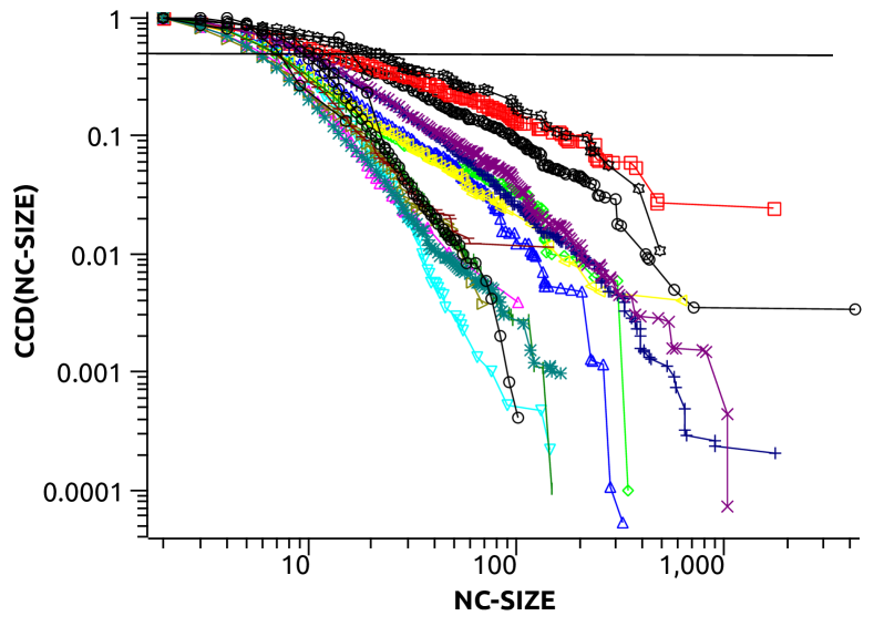
Figure 1: The complementary cumulative distribution of NC-SIZE for all graphs from our corpus. The solid horizontal line represents probability 0.5.

The average and maximal NC-LID in examined graphs are shown in Figure 2 sorted by the average NC-LID from the graph with the most compact natural communities to the graph with the most complex natural communities on average. The minimal NC-LID in all graphs is equal to 0, which is the lowest possible NC-LID. The lowest possible NC-LID corresponds to nodes whose local communities are strongly compact or convex in the sense that distances from a node to all nodes from its natural community are strictly smaller than distances from the node to nodes not belonging to its natural community (i.e., the shortest-path distance measure perfectly separates nodes from the natural community from outside nodes). It should be noticed that the average/maximal NC-LID does not steadily increase with the number of nodes nor with the density (average degree). In other words, smaller (resp., sparser) graphs may have more complex natural communities than larger (resp., denser) graphs. The social network of Florentine families has the lowest average NC-LID equal to 0.48. This NC-LID level means that approximately 38% of nodes within the shortest-path radius of the natural community of a randomly selected node do not belong to its natural community. BlogC has the most complex natural communities with the largest average NC-LID equal to 6.51. This NC-LID value corresponds to situations in which approximately 0.14% of nodes within the shortest-path radius of a natural community belong to the natural community.

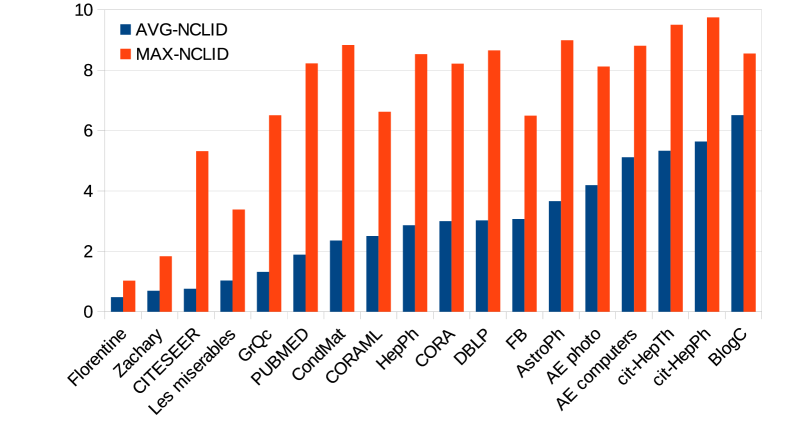
Figure 2: The average and the maximal NC-LID for graphs from our experimental corpus.

It is important to emphasize that NC-LID does not necessarily increase with NC-SIZE, i.e. smaller natural communities may be more complex than larger natural communities. Figure 3 shows the values of the Spearman correlation coefficient between NC-LID and NC-SIZE. It can be seen that for 8 (out of 18) graphs there is a positive correlation higher than 0.3. In those graphs larger natural communities tend to be more complex than smaller natural communities. The opposite tendency is present for 3 graphs (BlogC, FB and Zachary) in which smaller natural communities tend to be more complex than larger natural communities (a significant negative correlation lower than $-0.3$). For AE photo and PUBMED, Spearman correlation is close to 0 implying that larger natural communities do not tend to be neither more nor less complex than smaller natural communities.

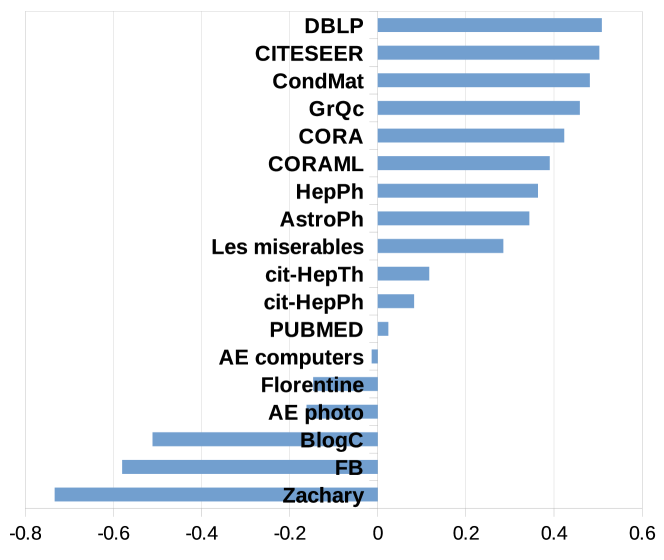
Figure 3: Spearman correlation between NC-LID and NC-SIZE.

To better understand the structural characteristics of nodes with complex natural communities we examine correlations between NC-LID and node centrality metrics quantifying structural importance of nodes in complex networks [35]. Node centrality metrics can be divided into two categories:

1. local metrics taking into account only links emanating from a node, and

2. global metrics reflecting the importance of the node considering the complete structure of the network.

The degree of a node (denoted by DEG) is the most basic local centrality metric. The main advantage of this metric is that it is easy and fast to compute. Nodes having high degree are also called hubs and they are especially important for the overall connectivity in scale-free networks and networks with heavy-tailed degree distributions, in general.

In our experimental evaluation we consider the following global centrality metrics:

• the shell or core index (denoted by CORE),

• eigenvector centrality (denoted by EVC),

• closeness centrality (denoted by CLO), and

• betweenness centrality (denoted by BET).

The core index is a metric related to the $k$-core decomposition of networks. The $k$-core is of a graph is its subgraph obtained by repeatedly removing nodes whose degree is smaller than $k$. The core index of a node is equal to $k$ if the node belongs to the $k$-core, but not to the $(k+1)$-core. Hubs predominantly connected to other hubs tend to have high values of this metric.

The eigenvector centrality metric is based on the principle that important nodes tend to be connected to other important nodes. This principle when expressed as a recurrence relation yields the eigenvector of the adjacency matrix as the vector expressing structural importance of nodes.

The intuition behind closeness centrality is that important nodes tend to be located in proximity to many other nodes. Formally, the closeness centrality of a node is inversely proportional to the total shortest-path distance between the node and all other nodes in the network.

The betweenness centrality of the node is the extent to which the node tends to be located on the shortest path between any two arbitrary nodes. Nodes with high betweenness tend to connect different cohesive node groups or clusters in the network, whereas nodes with high closeness tend to be the most central nodes in the most central clusters.

The values of Spearman correlation between NC-LID and node centrality metrics are shown in Table 2. Except in a few cases (EVC for Zachary; DEG and CORE for FB), there are positive Spearman correlations between NC-LID and node centrality metrics. It can be observed that DEG tends to have moderate Spearman correlations with NC-LID: for 7 graphs the correlation coefficient takes values between 0.4 and 0.6, for 9 graphs between 0.2 and 0.4 and only for 2 graphs there are weak correlations lower than 0.2. Moderate correlations lower than 0.6 are also present for BET. CORE, EVC and CLO tend to exhibit considerably higher correlations with NC-LID compared to DEG and BET. This result implies that nodes having complex local communities tend to be more globally than locally important. However, their global importance is not determined by their brokerage role in connecting different node clusters (high BET), but by their central positions (high CLO) in the most important clusters (high EVC) that are located in the core of the network (high CORE). For all datasets except one (Zachary, the smallest graph from our experimental corpus), CLO shows the strongest correlations with NC-LID: the correlation between NC-LID and CLO is very strong (higher than 0.8) for two graphs (CITESEER and GrQc), strong (between 0.6 and 0.8) for 7 graphs, moderate (between 0.4 and 0.6) for 6 graphs and only for 3 graphs correlations can be considered as low to moderate (values lower than 0.4 but higher than 0.2). This result indicates that high NC-LID nodes tend to be the most central nodes that have many long-range links, i.e., links whose removal drastically increases distances between nodes. Such long-range links are actually links connecting nodes belonging to different node clusters implying that high NC-LID nodes tend to be located in the most central node clusters (as also indicated by high correlations between NC-LID and CORE/EVC). Additionally, high NC-LID nodes tend to be well connected to both nodes from their own node clusters and nodes belonging to different node clusters which can explain high complexity or “concavity” of their natural communities since long-range links lead outside of the natural community of a node.

Table 2: Spearman correlations between NC-LID and various centrality metrics quantifying structural importance of nodes in complex networks.

Graph	DEG	CORE	EVC	CLO	BET
Zachary	0.113	0.137	-0.175	0.231	0.248
Florentine	0.200	0.429	0.435	0.535	0.240
Les miserables	0.302	0.269	0.441	0.444	0.349
CORAML	0.379	0.462	0.609	0.667	0.340
CITESEER	0.412	0.519	0.807	0.819	0.459
PUBMED	0.414	0.498	0.537	0.541	0.366
CORA	0.434	0.518	0.569	0.681	0.339
DBLP	0.536	0.615	0.712	0.742	0.397
AE photo	0.356	0.396	0.543	0.601	0.240
AE computers	0.441	0.478	0.564	0.588	0.283
BlogC	0.239	0.250	0.263	0.267	0.168
AstroPh	0.437	0.434	0.625	0.658	0.372
CondMat	0.398	0.392	0.634	0.689	0.355
GrQc	0.350	0.343	0.708	0.802	0.410
HepPh	0.367	0.376	0.652	0.691	0.338
cit-HepPh	0.360	0.407	0.446	0.465	0.226
cit-HepTh	0.472	0.508	0.563	0.578	0.266
FB	-0.004	-0.011	0.092	0.231	0.122

6.2 Node2vec Evaluation

In our experimental evaluation, node2vec was tuned by finding values of its hyper-parameters $p$ (return-back parameter) and $q$ (in-out parameter) that give embeddings maximizing the $F_{1}$ score in five different graph embedding dimensions (10, 25, 50, 100 and 200). As suggested by the authors of node2vec [5], for $p$ and $q$ we considered values in {0.25, 0.50, 1, 2, 4}, while the number of random walks per node and the length of each random walk were fixed to 10 and 80, respectively.

The results of node2vec tuning are presented in Table 3. The table shows maximal $F_{1}$ scores for graphs from our experimental corpus sorted from the largest to the lowest score, the dimension in which the maximal score is achieved (Dim.), the corresponding values of $p$ and $q$, and graph reconstruction evaluation metrics ($P$ – link precision and $R$ – link recall). It can be observed that the maximal $F_{1}$ score is in the range $[0.24,0.96]$. For the majority of graphs the maximal $F_{1}$ is larger than 0.5 implying that node2vec graph embeddings preserve the structure of input graphs to a very good extent. It can also be seen that link precision and recall tend to exhibit high correlations with $F_{1}$: a larger $F_{1}$ score in the vast majority of cases implies larger link precision and recall (the values of Person’s correlation coefficient between both link precision and recall on the one side and $F_{1}$ on the other side is equal to 0.98).

Table 3: Characteristics of the best node2vec embeddings (sorted from the highest to the lowest $F_{1}$ score).

Graph	Dim.	$p$	$q$	$P$	$R$	$F_{1}$
Florentine families	100	0.25	4	0.97	0.96	0.96
Les miserables	100	0.25	4	0.79	0.83	0.81
Zachary karate club	100	0.25	4	0.78	0.78	0.78
AstroPh	50	2	0.25	0.68	0.74	0.71
HepPh	25	0.5	0.25	0.68	0.73	0.71
CondMat	25	0.5	4	0.69	0.62	0.65
CORAML	25	0.5	0.25	0.63	0.67	0.65
FB	25	0.25	2	0.64	0.63	0.64
CORA	25	4	0.25	0.58	0.56	0.57
cit-HepTh	100	2	0.25	0.56	0.59	0.57
GrQc	10	0.25	2	0.61	0.53	0.56
cit-HepPh	100	4	0.25	0.54	0.51	0.53
AE photo	50	0.5	0.5	0.51	0.48	0.5
AE computers	50	4	0.25	0.49	0.42	0.45
DBLP	25	0.5	1	0.44	0.37	0.4
PUBMED	50	4	0.25	0.32	0.52	0.39
BlogC	50	0.25	0.25	0.28	0.22	0.25
CITESEER	10	0.5	0.25	0.23	0.24	0.24

High NC-LID nodes have more complex natural communities than low NC-LID nodes. It is reasonable to expect that high NC-LID will have higher reconstruction errors in graph embeddings due to more complex natural communities. To check this assumption we analyze Spearman correlations between NC-LID of nodes and their $F_{1}$ scores in the best node2vec embeddings obtained after hyper-parameter tuning. The values of the Spearman correlation coefficient between NC-LID and $F_{1}$ for all graphs from our experimental corpus are shown in Figure 4. It can be seen that for 15 (out of 18) graphs there are significant negative Spearman correlations ranging between $-0.2$ and $-0.4$. Consequently, it can be concluded that NC-LID is able to fairly accurately identify nodes that have high link reconstruction errors (please recall that lower $F_{1}$ scores imply higher link reconstruction errors).

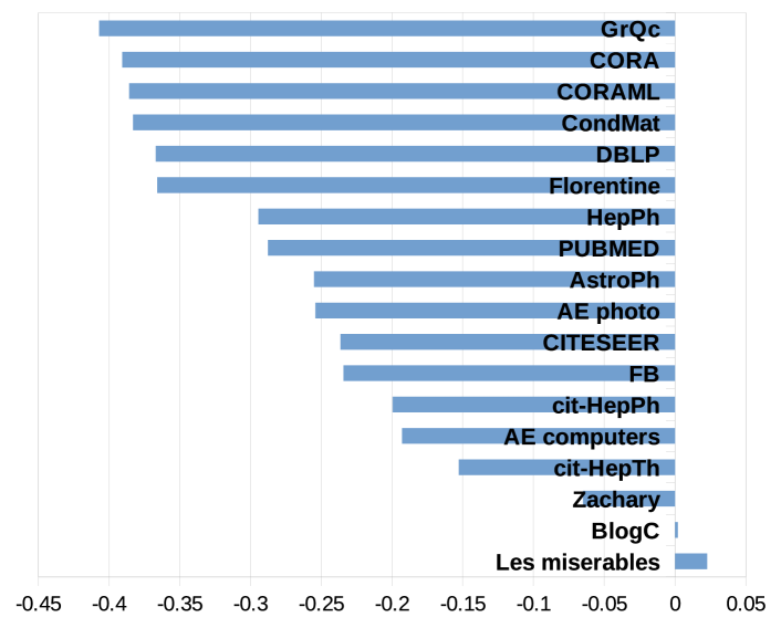
Figure 4: The Spearman correlation between NC-LID and $F_{1}$ scores in the best node2vec embeddings.

To further examine how NC-LID is related to the precision of links reconstructed from embeddings we divide nodes into two groups:

1. nodes having NC-LID above the average NC-LID (high NC-LID nodes, group $H$), and

2. nodes having NC-LID below the average NC-LID (low NC-LID nodes, group $L$).

Then, we compare $F_{1}$ scores of those two groups of nodes using the Mann-Whitney U (MWU) test [46]. The MWU test is a test of stochastic equality checking the null hypothesis stating that $F_{1}$ scores in $H$ do not tend to be neither greater nor smaller than $F_{1}$ scores in $L$. Additionally, we compute two probabilities of superiority reflecting tendencies of stochastic inequalities:

1. PS($H$) – the probability that a randomly selected node from $H$ has a higher $F_{1}$ than a randomly selected node form $L$,

2. PS($L$) - the probability that a randomly selected node from $L$ has a higher $F_{1}$ than a randomly selected node from $H$ ($\mbox{PS}(L)=1-\mbox{PS}(H)-P_{e}$, where $P_{e}$ is the probability of observing equal $F_{1}$ scores in $H$ and $L$).

The results of statistical testing and accompanying probabilities of superiority are presented in Table 4. $F_{1}(H)$ and $F_{1}(L)$ in Table 4 denote the average $F_{1}$ score for nodes in $H$ and $L$, respectively. $U$ is the value of the MWU test statistic and the null hypothesis of the test is accepted if the $p$-value of $U$ is higher than 0.05, which is also indicated by the ACC column in Table 4 (“yes” means that the null hypothesis is accepted). From the obtained results we can observe that the null hypothesis is accepted for the three smallest graphs: Zachary karate club, Les miserables and Florentine families. For those three graphs differences in $F_{1}$ scores of high and low NC-LID nodes are not statistically significant. For large graphs we have that $F_{1}$ scores of high NC-LID nodes tend to be significantly lower than $F_{1}$ scores of low NC-LID nodes: $F_{1}(H)<F_{1}(L)$ and $\mbox{PS}(H)\ll\mbox{PS}(L)$.

Table 4: Comparison of $F_{1}$ scores of high NC-LID nodes ($H$) and low NC-LID nodes ($L$) using the Mann-Whitney U test.

Graph	$F_{1}(H)$	$F_{1}(L)$	$U$	$p$	ACC	PS($H$)	PS($L$)
Zachary	0.70	0.71	132	0.44	yes	0.44	0.48
Les miserables	0.76	0.76	734	0.50	yes	0.47	0.47
Florentine	0.93	0.98	19	0.10	yes	0.07	0.39
CORAML	0.44	0.62	699380	$<0.01$	no	0.29	0.67
CITESEER	0.10	0.25	1707420	$<0.01$	no	0.19	0.31
AE photo	0.32	0.43	5239408	$<0.01$	no	0.36	0.64
AE computers	0.29	0.38	17900546	$<0.01$	no	0.38	0.61
PUBMED	0.19	0.32	31448278	$<0.01$	no	0.28	0.59
CORA	0.36	0.54	29695497	$<0.01$	no	0.28	0.68
DBLP	0.20	0.42	26684749	$<0.01$	no	0.25	0.57
BlogC	0.13	0.14	10915606	$<0.01$	no	0.45	0.49
AstroPh	0.55	0.65	32743550	$<0.01$	no	0.37	0.62
CondMat	0.45	0.62	42561679	$<0.01$	no	0.31	0.66
GrQc	0.35	0.57	2051967	$<0.01$	no	0.28	0.64
HepPh	0.53	0.66	12720029	$<0.01$	no	0.35	0.63
cit-HepPh	0.35	0.43	114704661	$<0.01$	no	0.39	0.60
cit-HepTh	0.41	0.47	79349590	$<0.01$	no	0.43	0.57
FB	0.51	0.59	1634998	$<0.01$	no	0.41	0.59

The next question we empirically address is whether NC-LID is a better indicator of nodes with low $F_{1}$ scores in node2vec embeddings than node centrality metrics. We have computed Spearman correlations (denoted by $\rho$) between node centrality metrics and NC-LID one one side and $F_{1}$ scores in the best node2vec embeddings on the other side for all graphs from our experimental corpus in order to determine which node metric has the strongest ability to point to nodes high link reconstruction errors. The obtained correlations are given in Table 5. The first thing that should be noticed is that only NC-LID exhibits negative correlations with $F_{1}$, whereas for node centrality metrics it can be observed both negative and positive correlations. For example, DEG exhibits a positive correlation with $F_{1}$ on Blog-catalog ($\rho$ = 0.306) and a negative correlation on DBLP ($\rho$ = $-0.398$). When a metric exhibits both negative and positive correlations with $F_{1}$ then it cannot be solely exploited to improve a graph embedding algorithm. In cases of strong positive correlations, high values of the metric indicate “good” nodes (nodes with low graph reconstruction errors), while in cases of strong negative correlations high values point out to “bad” nodes (nodes with high graph reconstruction errors).

Table 5: Spearman correlations between $F_{1}$ scores in the best node2vec embeddings and various metrics for nodes in complex networks including NC-LID.

Graph	NC-LID	DEG	CORE	EVC	CLO	BET
Zachary	$-0.065$	0.193	0.173	$-0.125$	$-0.03$	0.071
Florentine	$-0.367$	$-0.352$	$-0.423$	$-0.466$	$-0.25$	$-0.158$
Les miserables	$-0.045$	0.308	0.396	0.118	$-0.121$	0.002
CORAML	$-0.386$	$-0.112$	$-0.178$	$-0.318$	$-0.421$	$-0.129$
CITESEER	$-0.236$	$-0.161$	$-0.108$	$-0.307$	$-0.317$	$-0.215$
PUBMED	$-0.288$	$-0.252$	$-0.346$	$-0.165$	$-0.248$	$-0.257$
CORA	$-0.391$	$-0.215$	$-0.255$	$-0.271$	$-0.384$	$-0.251$
DBLP	$-0.367$	$-0.398$	$-0.438$	$-0.31$	$-0.362$	$-0.392$
AE photo	$-0.264$	0.088	0.053	$-0.122$	$-0.196$	$-0.026$
AE computers	$-0.204$	0.026	$-0.014$	$-0.15$	$-0.208$	$-0.021$
BlogC	0.002	0.306	0.305	0.286	0.269	0.304
AstroPh	$-0.255$	0.069	0.114	$-0.096$	$-0.132$	$-0.16$
CondMat	$-0.383$	$-0.109$	$-0.015$	$-0.219$	$-0.305$	$-0.377$
GrQc	$-0.407$	$-0.046$	0.036	$-0.269$	$-0.34$	$-0.358$
HepPh	$-0.294$	0.2	0.222	$-0.088$	$-0.109$	$-0.161$
cit-HepPh	$-0.199$	0.041	0.028	$-0.029$	$-0.098$	$-0.054$
cit-HepTh	$-0.153$	0.087	0.072	0.015	$-0.026$	0.009
FB	$-0.234$	0.452	0.449	0.157	0.06	0.166

Node metric $M_{1}$ better points to weak parts of a node2vec embedding (nodes with low $F_{1}$ scores) obtained from a graph $G$ compared to node metric $M_{2}$ if $M_{1}$ achieves stronger correlations with $F_{1}$ (by absolute value) than $M_{2}$ with $F_{1}$. In such cases we say that $M_{1}$ wins over $M_{2}$ on $G$. From the results shown in Table 4 it can be seen that:

1. When NC-LID wins over some other metric, it is always a winning situation with a significantly stronger negative correlation.

2. NC-LID achieves 13 wins over DEG. DEG wins only on 5 datasets: on 1 dataset with a significant positive correlation and on 4 datasets with significant negative correlations.

3. NC-LID wins 11 times over CORE. CORE is better than NC-LID on 7 datasets (including the three smallest graphs), 3 times with significant negative and 4 times with significant positive correlations.

4. NC-LID is better than EVC on 13 graphs. EVC wins 3 times with significant negative correlations and 2 times with significant positive correlation.

5. NC-LID has 12 wins over CLO. CLO is better on 6 datasets: 5 times with negative correlations and once with a significant positive correlation (on Blog-catalog which is a large graph).

6. NC-LID is better than BET 15 times. BET has only 3 wins over NC-LID (two times with positive and once with a negative correlation).

According to the number of wins, it can be concluded that NC-LID is a much better indicator of nodes with low $F_{1}$ scores in node2vec embeddings than node centrality metrics. Additionally, NC-LID can be computed more quickly than global centrality metrics. Finally, node centrality metrics in some cases are able to point to weak parts and in some other cases to good parts of node2vec embeddings. Therefore, they cannot be directly utilized to adjust node2vec parameters per node (the number and length of random walks) or pair of nodes (parameters controlling random walk biases) in contrast to NC-LID which always indicates bad parts of node2vec embeddings.

6.3 LID-elastic node2vec Evaluation

Our LID-elastic node2vec extensions are based on the premise that high NC-LID nodes have higher link reconstruction errors than low NC-LID nodes due to more complex natural communities. The quality of graph embeddings can be assessed by comparing original graphs to graphs reconstructed from embeddings. Let $G$ denote an arbitrary graph with $L$ links and let $E$ be an embedding constructed from $G$ using some graph embedding algorithm. Please recall that $E$ is actually a list of real-valued vectors of the same size (embedding dimension), one vector per node. The graph reconstructed from $E$ has the same number of links as $G$. The links in the reconstructed graph are formed by joining the $L$ closest vector pairs from $E$ by Euclidean distance. The below defined link reconstruction error metrics can be used to assess the quality of $E$ according to the principle that nodes close in $G$ should also be close in $E$.

Definition 1 (Link precision).

The link precision for node $n$, denoted by $P(n)$, is equal to the number of correctly reconstructed links incident to $n$ divided by the total number of links incident to $n$ in the reconstructed graph.

Definition 2 (Link recall).

The link recall for node $n$, denoted by $R(n)$, is the number of correctly reconstructed links incident to $n$ divided by the total number of links incident to $n$ in the original graph.

Definition 3 ($F_{1}$ score).

The $F_{1}$ score for node $n$ aggregates link precision and recall into a single measure by taking their harmonic mean, i.e.

$$F_{1}(n)=\frac{2\cdot P(n)\cdot R(n)}{P(n)+R(n)}.$$

Higher values of $P(n)$, $R(n)$ and $F_{1}(n)$ imply lower link reconstruction errors for $n$. The link reconstruction errors at the level of the whole graph can be obtained by taking averages across all nodes.

The obtained results of the evaluation of LID-elastic node2vec variants are summarized in Table 6. The table shows the best $F_{1}$ scores of node2vec (n2v), the dimensions in which they are achieved (Dim.), the best $F_{1}$ scores of LID-elastic node2vec variants and corresponding embedding dimensions. The column “Best” indicates the best graph embedding algorithm achieving the maximal $F_{1}$ score (i.e., the algorithm that better preserves the graph structure compared to the others) where rw denotes the first LID-elastic node2vec extension (lid-n2v-rw) and rwpq is the second extension (lid-n2v-rwpq). The column “I [%]” is the percentage improvement in $F_{1}$ of a better LID-elastic node2vec extension over the original node2vec.

Table 6: Comparison of Node2Vec and LID-elastic Node2Vec embeddings.

	n2v		lid-n2v-rw		lid-n2v-rwpq
Graph	$F_{1}$	Dim.	$F_{1}$	Dim.	$F_{1}$	Dim.	Best	I[%]
BlogC	0.247	50	0.363	100	0.2	100	rw	47.16
DBLP	0.403	25	0.441	25	0.531	50	rwpq	31.7
GrQc	0.563	10	0.707	25	0.657	50	rw	25.63
CITESEER	0.236	10	0.248	10	0.28	10	rwpq	18.69
Zachary	0.779	100	0.829	50	0.852	100	rwpq	9.41
PUBMED	0.394	50	0.431	50	0.42	50	rw	9.37
CondMat	0.653	25	0.696	50	0.702	50	rwpq	7.55
AE photo	0.495	50	0.52	50	0.487	50	rw	4.91
cit-HepPh	0.528	100	0.553	100	0.529	50	rw	4.8
AE computers	0.452	50	0.473	100	0.421	50	rw	4.67
CORA	0.572	25	0.595	50	0.59	50	rw	3.95
cit-HepTh	0.572	100	0.594	100	0.565	50	rw	3.9
FB	0.638	25	0.659	25	0.655	25	rw	3.22
Les miserables	0.81	100	0.799	100	0.832	200	rwpq	2.65
HepPh	0.708	25	0.724	50	0.7	25	rw	2.34
AstroPh	0.711	50	0.724	100	0.69	50	rw	1.78
CORAML	0.649	25	0.657	50	0.631	25	rw	1.28
Florentine	0.964	100	0.964	100	0.964	100	all	0

For Florentine families (the smallest graph in our experimental corpus) both LID-elastic node2vec extensions achieve the same $F_{1}$ score as node2vec. In all other cases at least one LID-elastic variant is better than node2vec. Both LID-elastic variants better preserve the graph structure than node2vec for 9 graphs (out of 18 in total). The lid-n2v-rw variant achieves the highest score $F_{1}$ for 12 graphs, while lid-n2v-rwpq wins on 5 graphs. Large improvements in $F_{1}$ scores are present for 4 graphs:

• lid-n2v-rw significantly outperforms node2vec on BlogC and GrQc by increasing $F_{1}$ by 47.16% and 25.63%, respectively, and

• lid-n2v-rwpq significantly outperforms node2vec on DBLP and CITESEER where $F_{1}$ is improved by 31.7% and 18.69%, respectively.

Considerable improvements in $F_{1}$ scores (approximately 5% or higher) can be also observed for 5 graphs (Zachary, PUBMED, CondMat, AE photo, cit-HepPh and AE computers). Therefore, it can be concluded that our LID-elastic node2vec extensions are able to improve node2vec embeddings with respect to graph reconstruction errors.

7 Conclusions and Future Work

In this paper we have discussed the notion of local intrinsic dimensionality in the context of graphs. Since graphs are dimensionless objects, existing LID models could be applied to graphs by computing LID estimators either on graph embeddings or on graph-based distances.

Inspired by the fundamental connection between the local intrinsic dimensionality and the discriminability of distance functions in Euclidean spaces, we have proposed the NC-LID metric quantifying the discriminability of the shortest path distance considering natural communities of nodes in graphs. It has been shown that NC-LID exhibits consistent and stronger correlations to link reconstruction errors in node2vec embeddings than five centrality measures commonly used to quantify structural importance of nodes in complex networks. This result implies that NC-LID is a better choice for designing elastic graph embedding algorithms than standard node centrality measures. Furthermore, we have evaluated two LID-elastic extensions of the node2vec graph embedding algorithm in which hyperparameters are personalized per node and adjusted according to their NC-LID values. Our experimental evaluation of the proposed LID-elastic extensions on 18 real-world graphs revealed that they are able to improve node2vec embeddings with respect to graph reconstruction errors.

The present research could be continued in several directions, some of them being theoretical and some having a more practical flavor. The first theoretical direction is to investigate possibilities for designing LID-related metrics reflecting the discriminability of graph-based distance functions considering expanding subgraph localities. In the same way as NC-LID, such metrics could be exploited to personalize and adjust hyperparameters of graph embedding algorithms. The second direction having a more applicative nature is to examine LID-elastic node2vec embeddings in the context of machine learning tasks on graph-structured data (e.g., node clustering, node classification and link prediction). Finally, the NC-LID measure (or its derivatives based on expanding subgraph localities) could be incorporated into the loss function of graph autoencoders and graph neural networks in order to obtain graph embeddings by LID-aware deep learning techniques.

References

- [1] M. Savić, V. Kurbalija, M. Radovanović, Local intrinsic dimensionality and graphs: Towards LID-aware graph embedding algorithms, in: N. Reyes, R. Connor, N. Kriege, D. Kazempour, I. Bartolini, E. Schubert, J.-J. Chen (Eds.), Similarity Search and Applications, Springer International Publishing, Cham, 2021, pp. 159–172. doi:10.1007/978-3-030-89657-7_13.
- [2] M. E. Houle, Dimensionality, discriminability, density and distance distributions, in: 2013 IEEE 13th International Conference on Data Mining Workshops, 2013, pp. 468–473. doi:10.1109/ICDMW.2013.139.
- [3] L. Amsaleg, O. Chelly, T. Furon, S. Girard, M. E. Houle, K.-i. Kawarabayashi, M. Nett, Estimating local intrinsic dimensionality, in: Proceedings of the 21th ACM SIGKDD International Conference on Knowledge Discovery and Data Mining, KDD ’15, Association for Computing Machinery, New York, NY, USA, 2015, p. 29–38. doi:10.1145/2783258.2783405.
- [4] A. Lancichinetti, S. Fortunato, J. Kertész, Detecting the overlapping and hierarchical community structure in complex networks, New Journal of Physics 11 (3) (2009) 033015. doi:10.1088/1367-2630/11/3/033015.
- [5] A. Grover, J. Leskovec, Node2vec: Scalable feature learning for networks, in: Proceedings of the 22nd ACM SIGKDD International Conference on Knowledge Discovery and Data Mining, KDD ’16, Association for Computing Machinery, New York, NY, USA, 2016, p. 855–864. doi:10.1145/2939672.2939754.
- [6] D. Knežević, J. Babić, M. Savić, M. Radovanović, Evaluation of LID-Aware Graph Embedding Methods for Node Clustering, in: T. Skopal, F. Falchi, J. Lokoč, M. L. Sapino, I. Bartolini, M. Patella (Eds.), Similarity Search and Applications, Springer International Publishing, Cham, 2022, pp. 222–233. doi:10.1007/978-3-031-17849-8_18.
- [7] M. E. Houle, Local intrinsic dimensionality I: An extreme-value-theoretic foundation for similarity applications, in: C. Beecks, F. Borutta, P. Kröger, T. Seidl (Eds.), Similarity Search and Applications, Springer International Publishing, Cham, 2017, pp. 64–79. doi:10.1007/978-3-319-68474-1_5.
- [8] M. E. Houle, Local intrinsic dimensionality II: Multivariate analysis and distributional support, in: C. Beecks, F. Borutta, P. Kröger, T. Seidl (Eds.), Similarity Search and Applications, Springer International Publishing, Cham, 2017, pp. 80–95. doi:10.1007/978-3-319-68474-1_6.
- [9] M. E. Houle, Local intrinsic dimensionality III: Density and similarity, in: S. e. a. Satoh (Ed.), Similarity Search and Applications, Springer International Publishing, Cham, 2020, pp. 248–260. doi:10.1007/978-3-030-60936-8_19.
- [10] M. E. Houle, H. Kashima, M. Nett, Generalized expansion dimension, in: 2012 IEEE 12th International Conference on Data Mining Workshops, 2012, pp. 587–594. doi:10.1109/ICDMW.2012.94.
- [11] L. Amsaleg, O. Chelly, M. E. Houle, K.-I. Kawarabayashi, M. Radovanović, W. Treeratanajaru, Intrinsic Dimensionality Estimation within Tight Localities, in: Proceedings of the 2019 SIAM International Conference on Data Mining, Society for Industrial and Applied Mathematics, 2019, pp. 181–189. doi:10.1137/1.9781611975673.21.
- [12] G. Casanova, E. Englmeier, M. E. Houle, P. Kröger, M. Nett, E. Schubert, A. Zimek, Dimensional testing for reverse k-nearest neighbor search, Proc. VLDB Endow. 10 (7) (2017) 769–780. doi:10.14778/3067421.3067426.
- [13] M. E. Houle, X. Ma, V. Oria, J. Sun, Efficient algorithms for similarity search in axis-aligned subspaces, in: A. J. M. Traina, C. Traina, R. L. F. Cordeiro (Eds.), Similarity Search and Applications, Springer International Publishing, Cham, 2014, pp. 1–12. doi:10.1007/978-3-319-11988-5_1.
- [14] M. E. Houle, X. Ma, M. Nett, V. Oria, Dimensional testing for multi-step similarity search, in: 2012 IEEE 12th International Conference on Data Mining, 2012, pp. 299–308. doi:10.1109/ICDM.2012.91.
- [15] M. E. Houle, V. Oria, A. M. Wali, Improving k-nn graph accuracy using local intrinsic dimensionality, in: C. Beecks, F. Borutta, P. Kröger, T. Seidl (Eds.), Similarity Search and Applications, Springer International Publishing, Cham, 2017, pp. 110–124. doi:10.1007/978-3-319-68474-1_8.
- [16] M. Aumüller, M. Ceccarello, The role of local dimensionality measures in benchmarking nearest neighbor search, Information Systems 101 (2021) 101807. doi:https://doi.org/10.1016/j.is.2021.101807.
- [17] L. Von Ritter, M. E. Houle, S. Günnemann, Intrinsic degree: An estimator of the local growth rate in graphs, in: S. Marchand-Maillet, Y. N. Silva, E. Chávez (Eds.), Similarity Search and Applications, Springer International Publishing, Cham, 2018, pp. 195–208. doi:10.1007/978-3-030-02224-2\_15.
- [18] M. E. Houle, E. Schubert, A. Zimek, On the correlation between local intrinsic dimensionality and outlierness, in: S. Marchand-Maillet, Y. N. Silva, E. Chávez (Eds.), Similarity Search and Applications, Springer International Publishing, Cham, 2018, pp. 177–191.
- [19] R. Becker, I. Hafnaoui, M. E. Houle, P. Li, A. Zimek, Subspace determination through local intrinsic dimensional decomposition: Theory and experimentation, arXiv 1907.06771.
- [20] X. Ma, Y. Wang, M. E. Houle, S. Zhou, S. M. Erfani, S. Xia, S. N. R. Wijewickrema, J. Bailey, Dimensionality-driven learning with noisy labels, in: J. G. Dy, A. Krause (Eds.), Proceedings of the 35th International Conference on Machine Learning, ICML 2018, Stockholmsmässan, Stockholm, Sweden, July 10-15, 2018, Vol. 80 of Proceedings of Machine Learning Research, PMLR, 2018, pp. 3361–3370.
-
[21]
X. Ma, B. Li, Y. Wang, S. M. Erfani, S. Wijewickrema, G. Schoenebeck, M. E.
Houle, D. Song, J. Bailey,
Characterizing adversarial
subspaces using local intrinsic dimensionality, in: International Conference
on Learning Representations, 2018.
URL https://openreview.net/forum?id=B1gJ1L2aW - [22] P. Goyal, E. Ferrara, Graph embedding techniques, applications, and performance: A survey, Knowledge-Based Systems 151 (2018) 78–94. doi:10.1016/j.knosys.2018.03.022.
- [23] H. Cai, V. W. Zheng, K. C.-C. Chang, A comprehensive survey of graph embedding: Problems, techniques, and applications, IEEE Transactions on Knowledge and Data Engineering 30 (9) (2018) 1616–1637. doi:10.1109/TKDE.2018.2807452.
- [24] I. Makarov, D. Kiselev, N. Nikitinsky, L. Subelj, Survey on graph embeddings and their applications to machine learning problems on graphs, PeerJ Computer Science 7. doi:10.7717/peerj-cs.357.
- [25] B. Perozzi, R. Al-Rfou, S. Skiena, Deepwalk: Online learning of social representations, KDD ’14, Association for Computing Machinery, New York, NY, USA, 2014, p. 701–710. doi:10.1145/2623330.2623732.
- [26] L. F. Ribeiro, P. H. Saverese, D. R. Figueiredo, Struc2vec: Learning node representations from structural identity, in: Proceedings of the 23rd ACM SIGKDD International Conference on Knowledge Discovery and Data Mining, KDD ’17, Association for Computing Machinery, New York, NY, USA, 2017, p. 385–394. doi:10.1145/3097983.3098061.
- [27] D. Wang, P. Cui, W. Zhu, Structural deep network embedding, in: Proceedings of the 22nd ACM SIGKDD International Conference on Knowledge Discovery and Data Mining, KDD ’16, Association for Computing Machinery, New York, NY, USA, 2016, p. 1225–1234. doi:10.1145/2939672.2939753.
- [28] S. Cao, W. Lu, Q. Xu, Deep neural networks for learning graph representations, in: Proceedings of the Thirtieth AAAI Conference on Artificial Intelligence, AAAI’16, AAAI Press, 2016, p. 1145–1152.
- [29] T. N. Kipf, M. Welling, Semi-Supervised Classification with Graph Convolutional Networks, in: 5th International Conference on Learning Representations, ICLR ’17, 2017.
- [30] W. L. Hamilton, R. Ying, J. Leskovec, Inductive representation learning on large graphs, in: Proceedings of the 31st International Conference on Neural Information Processing Systems, NIPS’17, Curran Associates Inc., Red Hook, NY, USA, 2017, p. 1025–1035.
- [31] D. J. Watts, S. H. Strogatz, Collective dynamics of ‘small-world’ networks, Nature 393 (6684) (1998) 440–442. doi:10.1038/30918.
- [32] A.-L. Barabasi, R. Albert, Emergence of scaling in random networks, Science 286 (5439) (1999) 509–512. doi:10.1126/science.286.5439.509.
- [33] R. R. Coifman, S. Lafon, Diffusion maps, Applied and Computational Harmonic Analysis 21 (1) (2006) 5–30, special Issue: Diffusion Maps and Wavelets. doi:10.1016/j.acha.2006.04.006.
- [34] S. Marchand-Maillet, O. Pedreira, E. Chávez, Structural intrinsic dimensionality, in: N. Reyes, R. Connor, N. Kriege, D. Kazempour, I. Bartolini, E. Schubert, J.-J. Chen (Eds.), Similarity Search and Applications, Springer International Publishing, Cham, 2021, pp. 173–185. doi:10.1007/978-3-030-89657-7_14.
- [35] M. Savić, M. Ivanović, L. C. Jain, Fundamentals of Complex Network Analysis, Springer International Publishing, Cham, 2019, pp. 17–56. doi:10.1007/978-3-319-91196-0_2.
- [36] S. Fortunato, Community detection in graphs, Physics Reports 486 (3) (2010) 75–174. doi:10.1016/j.physrep.2009.11.002.
- [37] A. Clauset, Finding local community structure in networks, Physical Review E 72 (2005) 026132. doi:10.1103/PhysRevE.72.026132.
- [38] J. P. Bagrow, Evaluating local community methods in networks, Journal of Statistical Mechanics: Theory and Experiment 2008 (05) (2008) P05001. doi:10.1088/1742-5468/2008/05/p05001.
- [39] F. Radicchi, C. Castellano, F. Cecconi, V. Loreto, D. Parisi, Defining and identifying communities in networks, Proceedings of the National Academy of Sciences 101 (9) (2004) 2658–2663. doi:10.1073/pnas.0400054101.
- [40] T. Mikolov, K. Chen, G. Corrado, J. Dean, Efficient estimation of word representations in vector space, in: Y. Bengio, Y. LeCun (Eds.), 1st International Conference on Learning Representations, ICLR 2013, Scottsdale, Arizona, USA, May 2-4, 2013, Workshop Track Proceedings, 2013.
- [41] O. Shchur, M. Mumme, A. Bojchevski, S. Günnemann, Pitfalls of graph neural network evaluation, Relational Representation Learning Workshop, NeurIPS 2018.
- [42] A. Bojchevski, S. Günnemann, Deep gaussian embedding of graphs: Unsupervised inductive learning via ranking, in: 6th International Conference on Learning Representations, ICLR 2018, Vancouver, BC, Canada, April 30 - May 3, 2018, Conference Track Proceedings, 2018.
- [43] J. Leskovec, A. Krevl, SNAP Datasets: Stanford large network dataset collection, http://snap.stanford.edu/data (Jun. 2014).
- [44] M. Savić, M. Ivanović, L. C. Jain, Analysis of Co-authorship Networks, Springer International Publishing, Cham, 2019, pp. 235–275. doi:10.1007/978-3-319-91196-0_7.
- [45] M. Savić, M. Ivanović, M. Radovanović, Z. Ognjanović, A. Pejović, T. Jakšić Krüger, The structure and evolution of scientific collaboration in serbian mathematical journals, Scientometrics 101 (3) (2014) 1805–1830. doi:10.1007/s11192-014-1295-6.
- [46] H. B. Mann, D. R. Whitney, On a Test of Whether one of Two Random Variables is Stochastically Larger than the Other, The Annals of Mathematical Statistics 18 (1) (1947) 50 – 60. doi:10.1214/aoms/1177730491.