Resummed heat-kernel and form factors for surface contributions: Dirichlet semitransparent boundary conditions
Abstract.
In this article we consider resummed expressions for the heat-kernel’s trace of a Laplace operator, the latter including a potential and imposing Dirichlet semitransparent boundary conditions on a surface of codimension one in flat space. We obtain resummed expressions that correspond to the first and second order expansion of the heat-kernel in powers of the potential. We show how to apply these results to obtain the bulk and surface form factors of a scalar quantum field theory in with a Yukawa coupling to a background. A characterization of the form factors in terms of pseudo-differential operators is given. Additionally, we discuss a connection between heat-kernels for Dirichlet semitransparent, Dirichlet and Robin boundary conditions.
1. Introduction
The relation between spectral functions and the quantum theory of fields has been a close one [1, 2], specially when considering external background fields, including electromagnetic fields [3] and curved spacetimes [4, 5, 6]. In particular, the (one-loop) quantum fluctuations are usually given in terms of operators of Laplace type, whose heat-kernels determine the one-loop effective action [7].
Recall that, given a Laplace-type operator defined on a real manifold of dimension , with or without boundary and the corresponding local boundary conditions, its heat-kernel (HK) is defined as . The theory establishes that under general conditions of smoothness of both the operator and the manifold, as the trace of the HK possesses the following expansion [8, 9, 10, 11]:
| (1.1) |
The function is called smearing function; its role is to give a precise mathematical meaning to terms that otherwise would be divergent (in physical terms, it acts as a regulator). The coefficients are called Gilkey–Seeley–DeWitt (GSDW) coefficients [1, 12, 9] and sometimes HAMIDEW, after Hadamard–Minakshisundaram–DeWitt [13]. They consist of volume and surface integrals, respectively over the bulk and the boundary of , of local invariants (including the smearing function). One can build them by considering a linear combination of all the possible invariants with the appropriate dimensions; the numerical coefficients in front of each single term are universal, i.e. independent of the problem at hand. Additionally, it can be shown that the HK corresponds to the solution of the following heat equation with initial localized conditions:
| (1.2) | ||||
In the last decades, the techniques in the computation of the GSDW coefficients have shown several advancements. During this period, the community has recognized the benefits of the joint use of index theorems and functorial techniques, together with the consideration of special cases [14].
Another important milestone has been the obtainment of partially resummed HK expansions. For example, it has been proved that, in the so-called covariant perturbation theory, one can resum all the derivatives acting on contributions to second [15, 16, 17] and third order in the curvatures [18, 19, 20, 21] (see also rederivations and physical consequences in [22, 23]). Other studied scenarios include resummations in abelian bundles [24], QED [25] , symmetric spaces [26, 27] and powers of the curvature [28, 29]; see Ref. [30] for additional considerations and [31, 32] for a related computation by Wigner.
In the above-mentioned developments, much more attention has been given to the case of manifolds without boundaries, being the study of HKs in manifolds with boundaries much less developed; a not exhaustive list of works which deal with the latter problem include Refs. [14, 33, 34, 35, 36, 37, 38, 39, 40] and references therein.
Trying to bring more balance into this scenario, in the present manuscript we will show how to obtain resummed expressions when Dirichlet semitransparent conditions on a flat surface are considered. According to the best of our knowledge, this is the first time that resummations for surface contributions of bulk quantities are studied.
The Dirichlet semitransparent boundary condition, also known as transmittal boundary condition [41], is equivalent to the introduction of a delta potential with support on a surface of codimension one [42, 43, 44]. The problem at hand has been widely studied in the realm of quantum field theories (QFTs); the interested reader may consult Refs. [45, 46, 47, 48, 49, 50, 51, 52, 53, 54, 55, 56]. Moreover, it has also been considered as a problem in a first quantization [57, 58, 59, 60, 61, 62, 63, 64, 65]. Recently, it has attracted much attention in connection with the related problem, see Refs. [66, 67, 68] for potentials and Ref. [69] for some generalizations of semitransparent boundary conditions.
To be precise, in the following we will thus be interested in an operator of Laplace type in -dimensional flat Euclidean space , whose potential is given by a sufficiently smooth function , summed to a Dirac delta function with support in a flat surface of codimension one (chosen without loss of generality as the plane):
| (1.3) |
Regarding its HK and physical applications, we may summarize the main results of the present article as follows:
- •
- •
- •
-
•
In Sec. 6, we apply the previous results to a scalar quantum field theory in dimensions, including a Yukawa coupling to a background field. We show how the resummed expansions may be applied to obtain the relevant form factors, which are shown to be pseudo-differential operators with symbols in for all (in the classification of L. Hörmander [70]).
In order to derive these results, we will require the potential in Eq. (1.3) to be positive and to decay rapidly enough at infinity. On the one hand, positivity can be guaranteed if one chooses a coupling and enforces ; otherwise, negative eigenvalues would threaten the definition of the Euclidean quantum field theory in Sec. 6 by creating instabilities. This requirement can be left aside in Secs. 2, 3 and 4, where we are just interested in the expression of the heat-kernel on the diagonal. On the other hand, the decay of should be understood as enabling an interpretation of the potential as a perturbation of the Laplacian-plus-delta operator.
2. A perturbative expansion of the heat-kernel in powers of
In the following sections, unless otherwise stated, we will refer to the case . We will comment on the possibility of applying our results to dimensional operators and come back to an arbitrary dimension in Sec. 6, when we will study a QFT. To fix the notation, we will call the support of the delta function; by analogy with the -dimensional case, for we will use the notation
| (2.1) |
Additionally, to enhance the readability of expressions we will make two definitions; one takes advantage of the symmetry under exchange of two variables and the other regards the derivative operator:
| (2.2) | ||||
| (2.3) |
As stated in the introduction, we will show how to compute the HK of the operator to all order in the parameter, albeit performing an expansion in powers of . To zeroth order in , the HK of the operator has already been computed in closed form in the literature, see Refs. [71, 72, 42]. Since it will prove crucial in our computations, we state this result.
Proposition 1.
The HK for the Laplace-type operator is given by
| (2.4) | ||||
where corresponds to the free HK in one-dimensional flat space.
Corollary 1.
Theorem 1.
If one adds a smearing function, then the trace of the operator ’s HK, under the assumptions around Eq. (1.3), is given by
| (2.6) | ||||
where we have defined the kernel
| (2.7) |
Corollary 2.
The only nonvanishing bulk GSDW coefficient associated to the operator , can be readily read from Eq. (LABEL:eq:trace_hk_zeroth). The surface contributions to the GSDW coefficients vanish for . For an odd integer, they read
| (2.8) | ||||
while, for and even, we have
| (2.9) | ||||
In order to check the validity of these results, one can compare the first coefficients with those previously computed in Ref. [41]. Notice also that the presence in the coefficients of a quotient involving derivatives is only apparent: considering as a symbol, one should first perform the division; the latter is exact for every , showing thus that the coefficients are made of local terms.
Remark 1.
Taking into account the universality of the numerical coefficients in the HK expansion, one can lift the one-dimensional results in Corollary 2 to arbitrary dimension, including the possibility of introducing additional geometrical features such as a curved manifold and a curved surface . Then:
-
(1)
The dependence on the dimension would be only through an overall factor , see Ref. [74].
-
(2)
The coefficients in Eqs. (2.8) and (2.9) would correspond to integrals over a -dimensional hypersurface with the appropriate measure. The variable may be taken as a space-dependent quantity (living on the surface ) and the derivatives in (2.8) and (2.9) become covariant derivatives normal to . The integrals over would be replaced by integrals over with the corresponding measure.
-
(3)
The additional geometrical features would manifest themselves as the appearance of new nonvanishing invariants contributing to the GSDW coefficients, including curvatures of the spacetime, the extrinsic curvature (also called second fundamental form) of the hypersurface , covariant derivatives in the directions tangent to acting on , etc.
The situation becomes more involved if one tries to perform the computation to higher orders in . One powerful technique that has been employed in the past as a way to develop asymptotic expansions of HKs has been the derivation of an integral equation for the HK, alternative to the differential equation (1.2); see for example [72, 15, 74, 75, 76]. Customarily, such an integral equation would involve the free HK; instead, in the present case will play its role.
Proposition 2.
The HK associated to satisfies the integral equation
| (2.10) | ||||
Proof.
The proof follows from direct application of the operator on both sides of Eq. (2.10), analogously to the usual case. After using the corresponding heat equation for , one can interpret . Using the symmetry of in its first two arguments after integrating by parts in and , one obtains then the desired result. ∎
The benefit of introducing the integral equation (2.10) is that it is particularly well-suited to perform a perturbative expansion in the potential. Indeed, by direct application of the heat equation and subsequent integrations by parts in the intermediate propertimes, one can prove the following corollary.
Corollary 3.
The HK of the operator can be expanded as a formal series in ,
| (2.11) | ||||
where the coefficients are made of iterated integrals of the potential and the heat-kernel :
| (2.12) | ||||
and .
In accordance with the hypotheses detailed in Sec. 1, all the integrals in Eq. (2.12) exist as long as the potential decays fast enough at infinity. This comment implies that this expansion is not valid for potentials that diverge at infinity, such as a harmonic one. One general situation in which this expansion is expected to be useful is that in which the potentials have two scales, one associated with its amplitude and the other one with its derivatives, being the latter much bigger than the former.
3. Heat-kernel’s trace: first order in
We will now show how to obtain a closed expression for the HK’s trace at linear order in . Let us first introduce, as usual, a smearing function , i.e. an infinitely differentiable function with compact support. Recall also that the imaginary error function and the complementary error function are defined in terms of the error function as
| (3.1) |
Theorem 2.
The trace of the operator ’s HK, under the assumptions around Eq. (1.3) and at linear order in , is given by
| (3.2) | ||||
where we have defined the kernels
| (3.3) | ||||
| (3.4) | ||||
Proof.
A direct way to prove this theorem is to consider Corollary 3 at linear order in . For the bulk contribution we have performed all the necessary integrations by part in order to remove all the derivatives acting on ; this is possible because of the assumed properties of and . Of course, a similar procedure can not be implemented for the boundary terms. ∎
Some comments are in order. First, the bulk contributions are independent of the delta potential. Indeed, if we expand for small coupling , we get
| (3.5) | ||||
These are standard formulae in the literature. As an example, the small-propertime () expansion in the second line is consistent with the results contained in [14] for the GSDW coefficients up to ; notice that, order by order in , it depends only on integer powers of , i.e. it is made of local contributions. Moreover, the formulae in Eq. (3.5) are compatible with the second order resummed result à la Barvisnky–Vilkovisky [15], see [14] and the discussion in Sec. 4 of the present manuscript.
Second, even if the presence of rational functions of the may induce one to think that nonlocalities may be present in the small-T expansion of the surface contributions, an explicit calculation shows that all the corresponding coefficients are made of local invariants. Even if the computations are lengthy, this can be straightforwardly seen from the following corollary of Theorem 2.
Corollary 4.
The surface contributions to the GSDW coefficients associated to the operator , at linear order in , vanish for . For an even number, they read
| (3.6) | ||||
while, for and odd, we have
| (3.7) | ||||
Remark 2.
The discussion in Remark 1 trivially extends to this order, with the addition that the coefficients will in general possess a functional dependence on derivatives of .
Coming back to Eq. (3.4), one can corroborate it by comparing with several previously known results. To begin with, if we consider a constant potential , then we obtain
| (3.8) |
which is the correct result since in that case we know the all-order expression . As an additional check, we can also remove the smearing function. In such a situation the result greatly simplifies.
Corollary 5.
Notice that, as previously, the denominator in Eq. (3.10) is formal: it is understood that one should first perform the division of the polynomials (which is exact for all ) before interpreting as a differential operator. The GSDW coefficients up to coincide with the corresponding ones in Ref. [74], while the term agrees with the result in Ref. [77].
One further comparison can be done employing the large expansion; we will postpone this analysis to Sec. 5.
4. Heat-kernel’s trace: second order in
Increasing the order in the potential substantially increases the difficulty in the computation of the HK’s trace. To simplify the results to quadratic order in and taking also into account that in physical applications it is customary to do so, in the following we will set the smearing function aside.
Theorem 3.
The trace of the operator ’s HK, under the assumptions around Eq. (1.3), at quadratic order in and neglecting total derivatives, is given by
| (4.1) | ||||
where the kernels are related to those present in the linear expansion:
| (4.2) |
Correspondingly, the GSDW coefficients read
| (4.3) |
Proof.
The correctness of Theorem 3 can be shown by appealing to the perturbative expansion in Eq. (2.12). At quadratic order in we notice that the only relevant variable is ; changing variables we thus get
| (4.4) | ||||
After replacing , this is proportional to the linear order expression with a smearing function, i.e. proportional to . The fact that we are neglecting total derivatives is a consequence of the integration by parts that we have performed in obtaining the kernels of the linear expression, cf. the proof of Theorem 2. Finally, the relation between the GSDW coefficients follows directly from the second equality in Eq. (4.2). ∎
Remark 3.
The discussion in Remark 2 trivially extends to this order.
Theorem 3 clarifies the comment made after Eq. (3.5): it can be easily checked that is the flat-space version of the Barvinsky–Vilkovisky kernel for the quadratic contribution in , which is proportional by a factor to . Alternatively, one can perform a small-propertime expansion and see that the first terms (up to order ) agree with the contributions listed in [14], of course after neglecting boundary terms.
An additional corroboration can be done by noting that in the limit when both factors becomes a constant we get
| (4.5) |
which again matches the expansion of , this time at quadratic order in . Instead, if just one of the becomes constant, we get the equivalent of Eq. (3.9):
| (4.6) | ||||
5. A connection with Dirichlet and Robin boundary conditions
5.1. Dirichlet boundary conditions
One further check of all the previous results can be performed considering the large- expansion. The first boundary contributions will be independent of and are expected to be related to the HK of a free Laplacian with Dirichlet boundary conditions. Indeed, it is well-known that in such a limit the operator acts as a free Laplacian on two half-spaces: they share as boundary, on which Dirichlet boundary conditions are imposed. This is to be expected on physical grounds, since as the layer foreseeable becomes impenetrable.
In the , one can obtain the following kernels, which define the trace of the heat-kernel up to quadratic order in the potential :
| (5.1) | ||||
| (5.2) | ||||
| (5.3) | ||||
At first order in the potential, the expression simplifies if we take the smearing function as the unit function; in that case, readable expressions are obtained for the surface contributions even at higher orders in :
| (5.4) | ||||
Taking the previous comments into account, the correctness of the coefficients multiplying the and factors can be respectively verified by comparing with the Dirichlet results in Refs. [14] and [78].
On the other side, at second order in we obtain that the surface terms are given by
| (5.5) | ||||
where is Dawson’s integral, . In the third line, we have rendered explicit the small-propertime expansion of the Dirichlet limit; one can readily see that the coefficient accompanying agrees with the expression in Ref. [78].
Notice that in all these expansions there appear no terms with an odd total number of derivatives. In fact, they simply vanish in our case, because of a cancellation between contributions from the two different semi-spaces: this is a consequence of the fact that the outward normal-pointing vector has different sign on the two sides of .
More generally, we can write down the expressions of the GSDW coefficients in the limit. For even they vanish, what can be simply proven by dimensional arguments, taking into account the precedent paragraph. For odd they are given by
| (5.6) | ||||
One can rephrase this result in the following way. Consider a smooth manifold with boundary . Let us call the boundary contributions to the th HK coefficient of the operator restricted to , with Dirichlet boundary conditions imposed on :
| (5.7) |
Then, the coefficients satisfy
| (5.8) |
where the dots denote terms with a functional structure different from the ones already present in .
5.2. Robin boundary conditions
We will dedicate this section to an elegant argument that links some heat-kernel coefficients for semitransparent conditions with those corresponding to Dirichlet and Robin boundary conditions.
To be more explicit, following Ref. [41], consider again a smooth manifold with boundary . Afterwards, glue two copies of the former along their common boundary, giving rise to the manifold . In this construction, take a Laplace operator , defined on the glued space , which satisfies the following two conditions: it implies semitransparent boundary conditions on (with parameter ) and reduces to the Laplace operator in both copies of . Additionally, consider a smearing function that is even upon reflections on . Under rather general assumptions, the formula proved in Ref. [41] is that the surface contributions to the heat-kernel coefficients satisfy
| (5.9) |
where imply Dirichlet boundary conditions for the operator and the following Robin ones111 The derivative in the normal direction to is denoted by . :
| (5.10) |
This result is applicable to our particular case, as long as one considers and that are even under reflection across . One should notice that the latter restriction means that terms containing or evaluated on the boundary, with odd, will trivially vanish. Taking this into account and considering the coefficients for Dirichlet and Robin boundary conditions listed in Ref. [14], it is a straightforward task to check that our first HK coefficients, both at zeroth and first order in , satisfy the relation (5.9).
Furthermore, one can invert the argument and obtain an infinite number of terms corresponding to HKs with Robin boundary conditions. Indeed, applying the result (5.9) to our operator (therefore assuming and even) and substituting the Dirichlet contribution with the help of Eq. (5.8), we obtain
| (5.11) |
where the coefficients in the RHS have been computed in the previous sections (up to second order in ) and the dots denote terms with a functional structure different from the ones already present in or .
6. Surface form factors in quantum field theory
As a simple, albeit conceptually rich application of the preceding results, let us now consider a quantum scalar field in -dimensional flat Euclidean space. We will couple it quadratically to the background field , according to the following action:
| (6.1) |
For a general discussion of this type of theories with and without the boundary term see respectively Refs. [51, 79, 80] and [81, 82]. Following the terminology in the QFT literature, the negative of the Laplacian will be denoted . As usually, the one-loop contribution to the effective action can be written in terms of the operator of quantum fluctuations [83],
| (6.2) |
either as a function of its determinant or, introducing an integral over Schwinger’s propertime , in terms of its HK:
| (6.3) | ||||
Recall that, as discussed in Sec. 1, in the following we will assume ; otherwise, the integrals in the propertime would be ill-defined.
Using the formulae for the HK developed in the previous sections, we can recast the one-loop effective action as222The zeroth order in can be read from Eq. (2.5).
| (6.4) | ||||
where and are called form factors. In Eq. (LABEL:eq:ea_form_factors) we are neglecting powers of the field higher than four, as well as all possible contributions involving its partial derivatives with respect to the directions tangent to the surface . For our purposes, this will turn out to be enough.
A closed expression for the form factors in arbitrary dimensions can be obtained; given that they are rather lengthy, we prefer to leave them to App. A. Instead, we will display here the corresponding formulae in dimensions, focusing on the terms that require to undergo a renormalization process; they are
| (6.5) | ||||
| (6.6) | ||||
| (6.7) | ||||
| (6.8) | ||||
| (6.9) | ||||
where is the Euler–Mascheroni constant and is an arbitrary constant with units of mass (introduced to render the argument of the logarithm in Eq. (6.3) dimensionless). Additionally, we have used dimensional regularization333In this simple example, it proves convenient to introduce dimensional regularization by just modifying the HK’s leading power of the propertime to be proportional to . Alternatively, one could modify the power of in the denominator of Eq. (6.3) to be and take afterwards the limit . and defined the functions
| (6.10) | ||||
| (6.11) | ||||
| (6.12) | ||||
6.1. The renormalization
The renormalization process follows now by absorbing the infinities of the theory into the dressed coupling constants. In the minimal subtraction (MS) scheme, one would just introduce counterterms to cancel the negative powers of ; this is the path followed for example in Ref. [51]. Explicitly, one should enlarge the Lagrangian of departure to include also terms with functional dependence equal to those of the necessary counterterms [7],
| (6.13) | ||||
The coefficients and correspond to the cosmological constant and the surface tension of (both up to some proportional factor), while , and are the mass of the field , the coupling of a quartic self-interaction for and a coupling of to the boundary. Notice that, in dimensional regularization and four dimensions, there would appear no further terms stemming from the neglected factors which are ; this can be seen by dimensional counting or by direct computation [51]. However, some further terms may be needed in other regularization schemes.
In dimensional regularization and a prescription in which we absorb all the independent one-loop corrections, the corresponding counterterms can be read from the Eqs. (6.5), (6.6), (6.7), (6.8) and (6.9), to wit:
| (6.14) | ||||
The renormalized parameters can be then defined as , where are the so-called bare parameters. Afterwards, one can write down a Callan–Symanzik equation involving the parameter ; the beta functions are as customarily defined as
| (6.15) |
A direct computation, taking into account that and are -independent, shows that in the present scheme the beta functions are444 Recall that we are not taking into account the quantum contributions of at this point; the formulae in (6.16) should be understood as the contributions to the beta functions derived from the quantum fluctuations of .
| (6.16) | ||||
6.2. An alternative renormalization scheme
In this subsection we will use a more physical scheme , in spirit similar to the discussions in Refs. [84, 82, 85, 86, 87, 88, 89, 90], noting that the functions and play the role of running coupling constants. Indeed, suppose that we measure the bulk quartic coupling of to have the value at a scale . Then its value at another scale will simply be given by , showing that our assertion is true (up to an experimentally determined constant). Additionally, the corresponding beta function reads
| (6.17) |
The situation is slightly different for , inasmuch as the relevant scale for its running is determined by the momentum perpendicular to the plate. On the one side, this means that our renormalization breaks Lorentz invariance, which was anyway already broken by the plate configuration. On the other side, this is not a consequence of having neglected in Eq. (LABEL:eq:ea_form_factors) terms involving partial derivatives with respect to the parallel directions: for fields vanishing at infinity, their contributions to will be boundary terms that simply vanish555 In general, this is no longer true for terms with higher powers of , such as the contribution in Eq. (LABEL:eq:ea_form_factors). . Analogously to the previous calculation, we can compute the beta function for in this scheme:
| (6.18) | ||||
It is important to notice that, as a consequence of discussion in the precedent paragraphs, we are lead to the conclusion that and do have physical meaning, differently to the case of (at least, as long as we do not include a dynamical gravity). The quantum field acts as a mediator between the boundary condition and the background , such that, if we try to confine , then we are also automatically enforcing to satisfy a boundary condition. The nature of the latter is encoded in the form factor .
As a last comment, it is interesting to study the asymptotic expansion of the running coupling constants for large and small (or masses), to wit:
| (6.19) |
| (6.20) |
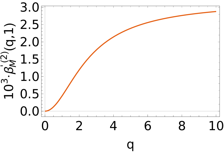
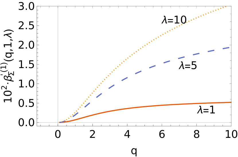
For large masses, they display the decoupling of the quantum field, analogue to the Appelquist and Carazzone result for QED [91] and generalizing the result for a Yukawa coupling without boundaries [92]. Additionally, the coefficients in the expansion are local. Instead, for large we see the nonlocal character of the runnings. In particular, we observe that both couplings diverge for . This implies that for situations involving high energy processes in the th direction, at the one-loop level, the field will have to obey a strong boundary condition on , i.e. almost Dirichlet. One can see that the plots in Fig. 1, which display the behaviours of the beta functions with the momentum scale and the coupling , are in agreement with the precedent description.
6.3. Formal aspects of the form factors
We will close this section with a short digression on a more mathematical description of the form factors. The ultimate goal will be to evidence one fact that is usually left aside in the literature: in general, form factors can be formally discussed in the frame of pseudo-differential operators. To begin, let us recall the following definitions borrowed from Ref. [70].
Definition 1 (Symbols).
Let and . The class of symbols consists of functions666 denotes the space of infinitely differentiable functions. (symbols) such that, for all multi-indices and , a constant exists for which
| (6.21) |
Definition 2 (Pseudo-differential operator).
If and777 is Schwartz’s space of functions whose derivatives are rapidly decreasing. , then
| (6.22) |
defines a function . One calls a pseudo-differential operator of order .
Proposition 3.
Consider couplings . Then the form factors for any , and therefore can be used to define pseudo-differential operators.
Proof.
Notice first that and have no dependence and plays the role of in Definition 2. For the terms made only of algebraic functions of , a bound as in Eq. (6.21) can be easily obtained; moreover, these terms are infinitely differentiable, since as assumption we have .
The terms that involve inverse hyperbolic functions display a twofold complication. First, they seem to have a singular behaviour for . This is just apparent, what can be shown using a Taylor expansion of the relevant functions around . Second, the corresponding large expansion yields terms, see Eqs. (6.19) and (6.20) below. However, after a first differentiation one obtains algebraic functions of and a bound as in (6.22) can be straightforwardly obtained. The fact that they belong to is thus also proved. ∎
Consequently, to analyze the form factors we can employ all the machinery of the theory of pseudo-differential operators. In particular, it is instructive to analyze under what circumstances the integrals in Eq. (LABEL:eq:ea_form_factors) are convergent. It is known that if the symbol belongs to the class , then the associated pseudo-differential operator is an endomorphism in the space of Lebesgue square-integrable functions, see [70, Theorem 18.1.11]. Although in the present case the behaviour for large prevents us from using this result, we can envisage two alternatives.
The first one is to stick to as the domain on which the form factors act, so that the image of the latter will have to be interpreted in terms of generalized functions. This has been followed for example in Ref. [82].
The remaining option is to restrict further the domain, in order to obtain a square-integrable function after applying the form factors [81]. If we follow this possibility, we can subtract to the form factors a term with an appropriate coefficient, obtaining thus a symbol in the class . The singular contribution is then given by a factor . As an example, in a sufficient, albeit not necessary set of conditions on that imply can be obtained using the lemma of Riemann–Lebesgue888 is the space of functions of a real variable with continuous derivatives up to second order. is the space of absolutely Lebesgue integrable functions of a real variable.: if and , then as desired.
7. Conclusions and outlook
From the mathematical point of view, we have determined an infinite number of GSDW coefficients. Bearing in mind the universality property discussed in Remarks 1, 2 and 3, these results may be an useful guide in more involved computations. We have also discussed, in Sec. 5, the connection of these computations with the GSDW of the Dirichlet and Robin problems.
As a next step it will be interesting to consider small curvature corrections to our problem. One could think for example in curving the plates, i.e. generating an extrinsic curvature on , or studying totally geodesic plates in a curved manifold. These problems may be analyzed either by expanding in powers of the curvature contributions or considering curved configurations in which form factors may be obtained to all order in the curvatures. In the latter case, homogeneous spaces are probably the most natural candidate.
From the physical point of view we have analyzed, as far as we know for the first time in the literature, surface form factors of a Yukawa theory and their implications. The most immediate consequence is the emergence of an energy-dependent semitransparent boundary condition satisfied by the background field.
One attractive possibility is to introduce a self-interacting term in the action (6.1). If one adds a quartic interaction, i.e. , then Eq. (6.2) acquires an additional term, which reads . The field is the classical field [7] and it is clear that its contribution to the effective action can be obtained by replacing . Doing so, one can readily compare the divergent terms with the counterterms found in Ref. [51]. By the discussion in the present manuscript, the semitransparent boundary condition satisfied by the classical field acquires then a dependence with the energy involved in a given physical process. However, a subtle point is that the classical field is expected to be discontinuous; in such case, taking into account the discussion in Sec. 6.3, the action of the form factors on it will have to be interpreted in terms of generalized functions and a detailed analysis will be required.
Natural generalizations include the study of more general physical models and boundary conditions. These lines are currently being explored.
Acknowledgements
S.A.F. is indebted to D.F. Mazzitelli and D. Vassilevich for interesting discussions; he is also grateful to J. Edwards, S. Evans and G. Schaller for their suggestions. S.A.F. acknowledges support from Helmholtz-Zentrum Dresden-Rossendorf (HZDR), PIP 11220200101426CO Consejo Nacional de Investigaciones Científicas y Técnicas (CONICET) and Project 11/X748, UNLP.
Appendix A Form factors in arbitrary dimensions
The explicit expressions for the form factors appearing in the effective action of Eq. (LABEL:eq:ea_form_factors), for arbitrary Euclidean spacetime dimensions , read
| (A.1) | ||||
| (A.2) | ||||
| (A.3) | ||||
| (A.4) | ||||
References
- [1] Bryce S. DeWitt “Dynamical Theory of Groups and Fields” New York: GordonBreach, Science Publishers Ltd., 1965
- [2] N.. Birrel and P… Davies “Quantum fields in curved space” Cambridge University Press, 1982
- [3] Julian S. Schwinger “On gauge invariance and vacuum polarization” In Phys. Rev. 82, 1951, pp. 664–679 DOI: 10.1103/PhysRev.82.664
- [4] J.. Dowker and Raymond Critchley “Effective Lagrangian and Energy Momentum Tensor in de Sitter Space” In Phys. Rev. D 13, 1976, pp. 3224 DOI: 10.1103/PhysRevD.13.3224
- [5] S.. Hawking “Zeta Function Regularization of Path Integrals in Curved Space-Time” In Commun. Math. Phys. 55, 1977, pp. 133 DOI: 10.1007/BF01626516
- [6] G.. Gibbons “Thermal Zeta Functions” In Phys. Lett. A 60, 1977, pp. 385–386 DOI: 10.1016/0375-9601(77)90026-3
- [7] Michael E. Peskin and Daniel V. Schroeder “An Introduction to quantum field theory” Reading, USA: Addison-Wesley, 1995
- [8] P. Greiner “An asymptotic expansion for the heat equation” In Arch. Ration. Mech. Anal. 41, 1971, pp. 163–218 DOI: 10.1007/BF00276190
- [9] Peter B. Gilkey “The Spectral geometry of a Riemannian manifold” In J. Diff. Geom. 10.4, 1975, pp. 601–618 DOI: 10.4310/jdg/1214433164
- [10] Peter B. Gilkey “Invariance Theory, the Heat Equation, and the Atiya-Singer Index Theorem” Boca Raton, Florida: CRC Press, 1995
- [11] Klaus Kirsten “Spectral functions in mathematics and physics” Boca Raton: Chapman & Hall/CRC, 2002
- [12] R.. Seeley “Complex powers of an elliptic operator” In Proc. Symp. Pure Math. 10, 1967, pp. 288–307
- [13] Gibbons, G.W. “Quantum field theory in curved spacetime” In General Relativity: An Einstein Centenary Survey Cambridge, UK: Univ. Pr., 1979, pp. 639
- [14] D.. Vassilevich “Heat kernel expansion: User’s manual” In Phys. Rept. 388, 2003, pp. 279–360 DOI: 10.1016/j.physrep.2003.09.002
- [15] A.. Barvinsky and G.. Vilkovisky “Beyond the Schwinger-Dewitt Technique: Converting Loops Into Trees and In-In Currents” In Nucl. Phys. B 282, 1987, pp. 163–188 DOI: 10.1016/0550-3213(87)90681-X
- [16] A.. Barvinsky and G.. Vilkovisky “Covariant perturbation theory. 2: Second order in the curvature. General algorithms” In Nucl. Phys. B 333, 1990, pp. 471–511 DOI: 10.1016/0550-3213(90)90047-H
- [17] Alessandro Codello and Omar Zanusso “On the non-local heat kernel expansion” In J. Math. Phys. 54, 2013, pp. 013513 DOI: 10.1063/1.4776234
- [18] A.. Barvinsky and G.. Vilkovisky “Covariant perturbation theory. 3: Spectral representations of the third order form-factors” In Nucl. Phys. B 333, 1990, pp. 512–524 DOI: 10.1016/0550-3213(90)90048-I
- [19] A.. Barvinsky, Yu.. Gusev, V.. Zhytnikov and G.. Vilkovisky “Covariant perturbation theory. 4. Third order in the curvature”, 1993 arXiv:0911.1168 [hep-th]
- [20] A.. Barvinsky, Yu.. Gusev, G.. Vilkovisky and V.. Zhytnikov “Asymptotic behaviors of the heat kernel in covariant perturbation theory” In J. Math. Phys. 35, 1994, pp. 3543–3559 DOI: 10.1063/1.530428
- [21] A.. Barvinsky, Yu.. Gusev, G.. Vilkovisky and V.. Zhytnikov “The Basis of nonlocal curvature invariants in quantum gravity theory. (Third order.)” In J. Math. Phys. 35, 1994, pp. 3525–3542 DOI: 10.1063/1.530427
- [22] I.. Avramidi “The Nonlocal Structure of the One Loop Effective Action via Partial Summation of the Asymptotic Expansion” In Phys. Lett. B 236, 1990, pp. 443–449 DOI: 10.1016/0370-2693(90)90380-O
- [23] I.. Avramidi “The Covariant Technique for Calculation of One Loop Effective Action” [Erratum: Nucl.Phys.B 509, 557–558 (1998)] In Nucl. Phys. B 355, 1991, pp. 712–754 DOI: 10.1016/0550-3213(91)90492-G
- [24] Ivan G. Avramidi and Guglielmo Fucci “Non-perturbative Heat Kernel Asymptotics on Homogeneous Abelian Bundles” In Commun. Math. Phys. 291, 2009, pp. 543–577 DOI: 10.1007/s00220-009-0804-6
- [25] V.. Gusynin and I.. Shovkovy “Derivative expansion of the effective action for QED in (2+1)-dimensions and (3+1)-dimensions” In J. Math. Phys. 40, 1999, pp. 5406–5439 DOI: 10.1063/1.533037
- [26] I.. Avramidi “A New algebraic approach for calculating the heat kernel in quantum gravity” In J. Math. Phys. 37, 1996, pp. 374–394 DOI: 10.1063/1.531396
- [27] I.. Avramidi “Covariant algebraic method for calculation of the low-energy heat kernel” In J. Math. Phys. 36, 1995, pp. 5055–5070 DOI: 10.1063/1.531371
- [28] Leonard Parker and David J. Toms “New Form for the Coincidence Limit of the Feynman Propagator, or Heat Kernel, in Curved Space-time” In Phys. Rev. D 31, 1985, pp. 953 DOI: 10.1103/PhysRevD.31.953
- [29] Ian Jack and Leonard Parker “Proof of Summed Form of Proper Time Expansion for Propagator in Curved Space-time” In Phys. Rev. D 31, 1985, pp. 2439 DOI: 10.1103/PhysRevD.31.2439
- [30] I.. Avramidi “Covariant techniques for computation of the heat kernel” In Rev. Math. Phys. 11, 1999, pp. 947–980 DOI: 10.1142/S0129055X99000295
- [31] Eugene P. Wigner “On the quantum correction for thermodynamic equilibrium” In Phys. Rev. 40, 1932, pp. 749–760 DOI: 10.1103/PhysRev.40.749
- [32] Y. Fujiwara, T.. Osborn and S… Wilk “WIGNER-KIRKWOOD EXPANSIONS” In Phys. Rev. A 25, 1982, pp. 14–34 DOI: 10.1103/PhysRevA.25.14
- [33] Klaus Kirsten, Peter Gilkey and Jeong-Hyeong Park “Heat content asymptotics for operators of Laplace type with spectral boundary conditions” In Lett. Math. Phys. 68, 2004, pp. 67–76 DOI: 10.1023/B:MATH.0000043236.80871.34
- [34] Giampiero Esposito, Guglielmo Fucci, Alexander Yu. Kamenshchik and Klaus Kirsten “Spectral asymptotics of Euclidean quantum gravity with diff-invariant boundary conditions” In Class. Quant. Grav. 22, 2005, pp. 957–974 DOI: 10.1088/0264-9381/22/6/005
- [35] Giampiero Esposito, Peter Gilkey and Klaus Kirsten “Heat kernel coefficients for chiral bag boundary conditions” In J. Phys. A 38, 2005, pp. 2259–2276 DOI: 10.1088/0305-4470/38/10/014
- [36] D.. McAvity and H. Osborn “A DeWitt expansion of the heat kernel for manifolds with a boundary” In Class. Quant. Grav. 8, 1991, pp. 603–638 DOI: 10.1088/0264-9381/8/4/008
- [37] D.. McAvity and H. Osborn “Asymptotic expansion of the heat kernel for generalized boundary conditions” In Class. Quant. Grav. 8, 1991, pp. 1445–1454 DOI: 10.1088/0264-9381/8/8/010
- [38] D.. McAvity and H. Osborn “Quantum field theories on manifolds with curved boundaries: Scalar fields” In Nucl. Phys. B 394, 1993, pp. 728–790 DOI: 10.1016/0550-3213(93)90229-I
- [39] A.. Barvinsky and D.. Nesterov “Quantum effective action in spacetimes with branes and boundaries” In Phys. Rev. D 73, 2006, pp. 066012 DOI: 10.1103/PhysRevD.73.066012
- [40] A.. Barvinsky and D.. Nesterov “The Schwinger-DeWitt technique for quantum effective action in brane induced gravity models” In Phys. Rev. D 81, 2010, pp. 085018 DOI: 10.1103/PhysRevD.81.085018
- [41] Peter B. Gilkey, Klaus Kirsten and Dmitri V. Vassilevich “Heat trace asymptotics with transmittal boundary conditions and quantum brane world scenario” In Nucl. Phys. B 601, 2001, pp. 125–148 DOI: 10.1016/S0550-3213(01)00083-9
- [42] S.. Franchino-Viñas and F.. Mazzitelli “Effective action for delta potentials: spacetime-dependent inhomogeneities and Casimir self-energy” In Phys. Rev. D 103.6, 2021, pp. 065006 DOI: 10.1103/PhysRevD.103.065006
- [43] M. Asorey, A. Ibort and G. Marmo “Global theory of quantum boundary conditions and topology change” In Int. J. Mod. Phys. A 20, 2005, pp. 1001–1026 DOI: 10.1142/S0217751X05019798
- [44] Sergio Albeverio, Friedrich Gesztesy, Raphael Høegh-Krohn and Helge Holden “Solvable Models in Quantum Mechanics” Springer-Verlag New York Inc., 1988 DOI: https://doi.org/10.1007/978-3-642-88201-2
- [45] Cesar D. Fosco and Francisco D. Mazzitelli “Casimir energy due to inhomogeneous thin plates” In Phys. Rev. D 101.4, 2020, pp. 045012 DOI: 10.1103/PhysRevD.101.045012
- [46] C.. Fosco, A. Giraldo and F.. Mazzitelli “Dynamical Casimir effect for semitransparent mirrors” In Phys. Rev. D 96.4, 2017, pp. 045004 DOI: 10.1103/PhysRevD.96.045004
- [47] Prachi Parashar, Kimball A. Milton, K.. Shajesh and Iver Brevik “Electromagnetic -function sphere” In Phys. Rev. D 96.8, 2017, pp. 085010 DOI: 10.1103/PhysRevD.96.085010
- [48] Cesar D. Fosco, Fernando C. Lombardo and Francisco D. Mazzitelli “Quantum dissipative effects in moving imperfect mirrors: sidewise and normal motions” In Phys. Rev. D 84, 2011, pp. 025011 DOI: 10.1103/PhysRevD.84.025011
- [49] C.. Fosco, F.. Lombardo and F.. Mazzitelli “Quantum dissipative effects in moving mirrors: A Functional approach” In Phys. Rev. D 76, 2007, pp. 085007 DOI: 10.1103/PhysRevD.76.085007
- [50] Kimball A. Milton and Jef Wagner “Exact Casimir interaction between semitransparent spheres and cylinders” In Phys. Rev. D 77, 2008, pp. 045005 DOI: 10.1103/PhysRevD.77.045005
- [51] Michael Bordag and D.. Vassilevich “Nonsmooth backgrounds in quantum field theory” In Phys. Rev. D 70, 2004, pp. 045003 DOI: 10.1103/PhysRevD.70.045003
- [52] N. Graham, R.. Jaffe, V. Khemani, M. Quandt, M. Scandurra and H. Weigel “Calculating vacuum energies in renormalizable quantum field theories: A New approach to the Casimir problem” In Nucl. Phys. B 645, 2002, pp. 49–84 DOI: 10.1016/S0550-3213(02)00823-4
- [53] Ian G Moss “Heat kernel expansions for distributional backgrounds” In Phys. Lett. B 491, 2000, pp. 203–206 DOI: 10.1016/S0370-2693(00)00966-7
- [54] Valeri P. Frolov and D. Singh “Quantum effects in the presence of expanding semitransparent spherical mirrors” In Class. Quant. Grav. 16, 1999, pp. 3693–3716 DOI: 10.1088/0264-9381/16/11/315
- [55] Michael Bordag, K. Kirsten and D. Vassilevich “On the ground state energy for a penetrable sphere and for a dielectric ball” In Phys. Rev. D 59, 1999, pp. 085011 DOI: 10.1103/PhysRevD.59.085011
- [56] Sergei N. Solodukhin “Exact solution for a quantum field with delta - like interaction” In Nucl. Phys. B 541, 1999, pp. 461–482 DOI: 10.1016/S0550-3213(98)00789-5
- [57] Christian Grosche “Path Integrals for Potential Problems With Delta Function Perturbation” In J. Phys. A 23, 1990, pp. 5205–5234
- [58] S.V. Lawande and K.V. Bhagwat “Feynman propagator for the -function potential” In Physics Letters A 131.1, 1988, pp. 8–10 DOI: https://doi.org/10.1016/0375-9601(88)90622-6
- [59] E B Manoukian “Explicit derivation of the propagator for a Dirac delta potential” In Journal of Physics A: Mathematical and General 22.1 IOP Publishing, 1989, pp. 67–70 DOI: 10.1088/0305-4470/22/1/013
- [60] J. Farias “Simple exact solution of the one-dimensional Schrödinger equation with continuous plus -function potentials of arbitrary position and strength” In Phys. Rev. A 22 American Physical Society, 1980, pp. 765–766 DOI: 10.1103/PhysRevA.22.765
- [61] John F. Reading and James L. Sigel “Exact Solution of the One-Dimensional Schrödinger Equation with -Function Potentials of Arbitrary Position and Strength” In Phys. Rev. B 5 American Physical Society, 1972, pp. 556–565 DOI: 10.1103/PhysRevB.5.556
- [62] R E Crandall “Combinatorial approach to Feynman path integration” In Journal of Physics A: Mathematical and General 26.14 IOP Publishing, 1993, pp. 3627–3648 DOI: 10.1088/0305-4470/26/14/024
- [63] M.. Goovaerts and F. Broeckx “Analytical Treatment of a Periodic -Function Potential in the Path-Integral Formalism” In SIAM Journal on Applied Mathematics 45.3 Society for IndustrialApplied Mathematics, 1985, pp. 479–490 URL: http://www.jstor.org/stable/2101725
- [64] Ilaria Cacciari and Paolo Moretti “Propagator for the double delta potential” In Physics Letters A 359.5, 2006, pp. 396–401 DOI: https://doi.org/10.1016/j.physleta.2006.06.061
- [65] Ilaria Cacciari and Paolo Moretti “On a class of integral equations having application in quantum dynamics” In Journal of Physics A: Mathematical and Theoretical 40.23 IOP Publishing, 2007, pp. F421–F426 DOI: 10.1088/1751-8113/40/23/f01
- [66] Ines Cavero-Pelaez, Jose M. Munoz-Castaneda and Cesar Romaniega “Casimir energy for concentric - spheres” In Phys. Rev. D 103.4, 2021, pp. 045005 DOI: 10.1103/PhysRevD.103.045005
- [67] J.. Munoz-Castaneda, L. Santamaria-Sanz, M. Donaire and M. Tello-Fraile “Thermal Casimir effect with general boundary conditions” In Eur. Phys. J. C 80.8, 2020, pp. 793 DOI: 10.1140/epjc/s10052-020-8348-1
- [68] M. Bordag, J.. Muñoz-Castañeda and L. Santamaría-Sanz “Free energy and entropy for finite temperature quantum field theory under the influence of periodic backgrounds” In Eur. Phys. J. C 80.3, 2020, pp. 221 DOI: 10.1140/epjc/s10052-020-7783-3
- [69] N. Ahmadiniaz, S.. Franchino-Viñas, L. Manzo and F.. Mazzitelli “Local Neumann semitransparent layers: Resummation, pair production, and duality” In Phys. Rev. D 106.10, 2022, pp. 105022 DOI: 10.1103/PhysRevD.106.105022
- [70] L. Hörmander “The analysis of linear partial differential operators III” Heidelberg: Springer-Verlag, 2007
- [71] D. Bauch “The path integral for a particle moving in a -function potential” In Il Nuovo Cimento B (1971-1996) 85, 1985, pp. 118–124 DOI: 10.1007/BF02721525
- [72] B. Gaveau and L.. Schulman “Explicit time-dependent Schrodinger propagators” In Journal of Physics A: Mathematical and General 19.10 IOP Publishing, 1986, pp. 1833–1846 DOI: 10.1088/0305-4470/19/10/024
- [73] Jose M. Munoz-Castaneda, J. Mateos Guilarte and A. Mosquera “Quantum vacuum energies and Casimir forces between partially transparent -function plates” In Phys. Rev. D 87.10, 2013, pp. 105020 DOI: 10.1103/PhysRevD.87.105020
- [74] Michael Bordag and D.. Vassilevich “Heat kernel expansion for semitransparent boundaries” In J. Phys. A 32, 1999, pp. 8247–8259 DOI: 10.1088/0305-4470/32/47/304
- [75] Michael Bordag, D. Vassilevich, H. Falomir and E.. Santangelo “Multiple reflection expansion and heat kernel coefficients” In Phys. Rev. D 64, 2001, pp. 045017 DOI: 10.1103/PhysRevD.64.045017
- [76] Michael Bordag, H. Falomir, E.. Santangelo and D.. Vassilevich “Boundary dynamics and multiple reflection expansion for Robin boundary conditions” In Phys. Rev. D 65, 2002, pp. 064032 DOI: 10.1103/PhysRevD.65.064032
- [77] S.. Franchino-Vinas and P… Pisani “Semi-transparent Boundary Conditions in the Worldline Formalism” In J. Phys. A 44, 2011, pp. 295401 DOI: 10.1088/1751-8113/44/29/295401
- [78] Thomas P. Branson, Peter B. Gilkey and Dmitri V. Vassilevich “The Asymptotics of the Laplacian on a manifold with boundary. 2” In Boll. Union. Mat. Ital. B 11, 1997, pp. 39–67 arXiv:hep-th/9504029
- [79] D.. Toms “Zeta-function regularization of the effective action for a delta-function potential” In Phys. Lett. B 632, 2006, pp. 422–426 DOI: 10.1016/j.physletb.2005.10.031
- [80] David J. Toms “Renormalization and vacuum energy for an interacting scalar field in a -function potential” In J. Phys. A 45, 2012, pp. 374026 DOI: 10.1088/1751-8113/45/37/374026
- [81] Francisco D. Mazzitelli, Jean Paul Nery and Alejandro Satz “Boundary divergences in vacuum self-energies and quantum field theory in curved spacetime” In Phys. Rev. D 84, 2011, pp. 125008 DOI: 10.1103/PhysRevD.84.125008
- [82] S.. Franchino-Viñas, M.. Mantiñan and F.. Mazzitelli “Quantum vacuum fluctuations and the principle of virtual work in inhomogeneous backgrounds” In Phys. Rev. D 105.8, 2022, pp. 085023 DOI: 10.1103/PhysRevD.105.085023
- [83] C. Itzykson and J.. Zuber “Quantum Field Theory” New York: McGraw-Hill Inc., 1980
- [84] E.. Gorbar and Ilya L. Shapiro “Nonlocality of quantum matter corrections and cosmological constant running” In JHEP 07, 2022, pp. 103 DOI: 10.1007/JHEP07(2022)103
- [85] Sebastián A. Franchino-Viñas, Tibério Paula Netto and Omar Zanusso “Vacuum effective actions and mass-dependent renormalization in curved space” In Universe 5.3, 2019, pp. 67 DOI: 10.3390/universe5030067
- [86] Sebastián A. Franchino-Viñas, Tibério Paula Netto, Ilya L. Shapiro and Omar Zanusso “Form factors and decoupling of matter fields in four-dimensional gravity” In Phys. Lett. B 790, 2019, pp. 229–236 DOI: 10.1016/j.physletb.2019.01.021
- [87] John F. Donoghue and Basem Kamal El-Menoufi “Covariant non-local action for massless QED and the curvature expansion” In JHEP 10, 2015, pp. 044 DOI: 10.1007/JHEP10(2015)044
- [88] M. Asorey, E.. Gorbar and I.. Shapiro “Universality and ambiguities of the conformal anomaly” In Class. Quant. Grav. 21, 2003, pp. 163–178 DOI: 10.1088/0264-9381/21/1/011
- [89] Eduard V. Gorbar and Ilya L. Shapiro “Renormalization group and decoupling in curved space. 2. The Standard model and beyond” In JHEP 06, 2003, pp. 004 DOI: 10.1088/1126-6708/2003/06/004
- [90] E.. Gorbar and I.. Shapiro “Renormalization group and decoupling in curved space” In JHEP 02, 2003, pp. 021 DOI: 10.1088/1126-6708/2003/02/021
- [91] Thomas Appelquist and J. Carazzone “Infrared Singularities and Massive Fields” In Phys. Rev. D 11, 1975, pp. 2856 DOI: 10.1103/PhysRevD.11.2856
- [92] Antonio Ferreiro, Sergi Nadal-Gisbert and José Navarro-Salas “Renormalization, running couplings, and decoupling for the Yukawa model in a curved spacetime” In Phys. Rev. D 104.2, 2021, pp. 025003 DOI: 10.1103/PhysRevD.104.025003