Pareto front analysis and multi-objective Bayesian optimization for ($R$, $Z$)(Fe,Co,Ti)₁₂ ($R$ = Y, Nd, Sm; $Z$ = Zr, Dy)

Abstract

We propose a scheme for investigating the correlation and trade-off among target variables using a multi-objective Bayesian optimization (MBO). We discuss the features of the Pareto front (PF) of ThMn₁₂-type compounds, ($R$, $Z$)(Fe,Co,Ti)₁₂ ($R$ = Y, Nd, Sm; $Z$ = Zr, Dy) in terms of magnetization, Curie temperature, and a price index by using data from first-principles calculations, and we extract the trade-off relations from the analysis. We show that the trade-off relationships can be used to determine changes in the controllable variables by using partial least squares regression. For example, the tendency toward low cost and high Curie temperature is related to the reduction in Dy and increase in Co. We also discuss the efficiency of MBO as a practical scheme to obtain the features of the PF. We show that MBO can offer an approximated set for the PF even when obtaining the true PF is difficult.

I Introduction

Magnet compounds with the ThMn12 structure have attracted attention as a potential main phase for high-performance permanent magnets Ohashi et al. (1988a, b); Yang et al. (1988); Verhoef et al. (1988); De Mooij and Buschow (1988); Buschow (1988); Jaswal et al. (1990); Coehoorn (1990); Buschow (1991); Sakurada et al. (1992); Sakuma (1992); Asano et al. (1993); Akayama et al. (1994); Kuz’min et al. (1999); Gabay et al. (2016); Körner et al. (2016); Ke and Johnson (2016); Fukazawa et al. (2017, 2019a). Hirayama et al. Hirayama et al. (2015a, b) synthesized a NdFe12 film and reported that the nitrogenated film exhibited a higher anisotropy field and magnetization than Nd2Fe14B, which is the main phase of the Nd magnet. However, NdFe12 has not been found as a homogeneous bulk material.

In the development of functional materials, the substitution of elements in known materials is a promising strategy. Elements in $R$Fe12 ($R$: rare earth) could be substituted to achieve higher performance and thermodynamic stability. Hirayama et al. reported that introducing Co to a SmFe12 film increased the Curie temperature and magnetization at room temperature. Ti stabilizes the ThMn12 structure, and bulk $R$Fe11Ti can be synthesized Ohashi et al. (1987, 1988a); De Mooij and Buschow (1988). However, Ti doping greatly reduces the magnetization owing to substitution of Fe and antiferromagnetic coupling between Ti and Fe. Zr has also been studied extensively as a stabilizer that dopes the $R$ site, which can avoid reduction of the magnetization caused by substitution at the Fe site Suzuki et al. (2014); Sakuma et al. (2016); Kuno et al. (2016); Suzuki (2017).

We also conducted several theoretical studies to search for performance-enhancing and stabilizing elements using first-principles calculations. We investigated the formation energy of NdFe11$M$ from the unary phases for $M$ = Ti–Zn and proposed that Co can stabilize the ThMn12 structure Harashima et al. (2016). We examined the stability of non-stoichiometric doped systems of the ThMn12 phase, where the phase competition with the Th2Zn17-structure phase was considered. This result suggests that Co alone does not function as a stabilizer; however, co-doping with Zr and Co may stabilize the ThMn12 structure Fukazawa et al. (2021). For $R$-site doping, we have studied $R$Fe12 with $R$ = La, Pr, Nd, Sm, Gd, Dy, Ho, Er, Tm, Lu, Y, and Sc and proposed some rare-earth elements, including Dy, as possible stabilizers Harashima et al. (2018).

Motivated by these works, in this study, we consider multiple doping, and we approach the search for optimal dopants and their concentration as an optimization problem. Machine learning techniques can deal well with this type of optimization problem, and several studies have applied these techniques to materials exploration Ueno et al. (2016); Ju et al. (2017); Kikuchi et al. (2018); Yuan et al. (2018). For optimizing the chemical composition of non-stoichiometric systems, we have been developing methods using Bayesian optimization combined with coherent potential approximation in first-principles calculations Fukazawa et al. (2019b, 2022). We have demonstrated that optimization with respect to chemical composition for a single target variable can be performed efficiently with these techniques, and that high-scored materials can be obtained with a small number of data acquisition processes.

In this paper, we consider a multi-objective optimization problem, where multiple target variables are considered simultaneously. In this type of problem, most of the data points are inferior to other data points with respect to all target variables, and these inferior data points are of much less interest.

The other important data points are called the Pareto front (PF). We focus on the PF with respect to the magnetization, the Curie temperature, and a price index as target variables in our analysis of first-principles data of (R,Z)(Fe,Co,Ti)12 with the ThMn12 structure. By using principal component analysis (PCA) and partial least squares (PLS) regression, we determine how the distribution of the PF is different from that of all data points, and how the information of the PF can be used to investigate the trade-offs among the target variables.

However, in practical applications, obtaining the PF itself can be difficult. We discuss the use of multi-objective Bayesian optimization (MBO) for the problem, and find that MBO is substantially more efficient than random sampling. We also propose that MBO can be used as an efficient sampling method for capturing the features of the PF.

Figure 1 summarizes our framework as a flow chart. First, the user prepares a list of candidate materials for which they want to obtain the PF. Then, with the combination of a multiple-objective Bayesian optimizer and a first-principles simulator, an approximate PF is efficiently obtained. We discuss the accuracy and the efficiency of this part of the framework in Section III.2. After an adequate PF is obtained, correlation analysis is performed to visualize or quantify the trade-off between the target variables. Control variable analysis can also be performed to determine how the target variables can be changed along the PF by changing the controllable parameters. As an example, in Section III.1, we see the possibility that an acceptable compromise on the performance leads to a large reduction in the price, and how the dopants and their concentration should be chosen.

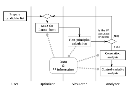
Figure 1: Work and data flow in the framework for PF analysis.

II Methodology

We use our data set for (R_$1-\alpha$$Z$_$\alpha$)(Fe_$1-\beta$Co_$\beta$)_$12-\gamma$Ti_$\gamma$ ($R$ = Y, Nd, Sm; $Z$ = Zr, Dy; $\alpha$ = 0–1; $\beta$ = 0–1; $\gamma$ = 0–2) obtained by first-principles calculations based on density functional theory within the local density approximation Hohenberg and Kohn (1964); Kohn and Sham (1965). The data set consists of 3630 data points. We use AkaiKKR (MACHIKANEYAMA) in the data acquisition, which is based on the Korringa-Kohn-Rostoker Green function method Korringa (1947); Kohn and Rostoker (1954). The lattice constants are determined by linear interpolation from those for $R$Fe12, $R$Fe11Ti, $Z$Fe12, $Z$Fe11Ti, and $R$Co12. The f-electrons in Nd, Sm, and Dy are treated as open cores Jensen and Mackintosh (1991); Locht et al. (2016); Richter (1998), and the self-interaction correction Perdew and Zunger (1981) is applied. In treating the randomness from the doping, we use coherent potential approximation Soven (1970); Shiba (1971).

Magnetization values are calculated from the magnetic moment and the volume. The Curie temperatures are obtained within the mean field approximation from the Heisenberg Hamiltonian, the coupling parameters of which are determined by Liechtenstein’s formula Liechtenstein et al. (1987). We fix the price indices for the elements to 0.24 for Y, 6.3 for Nd, 0.28 for Sm, 0.0056 for Zr, 35 for Dy, 0.0056 for Fe, 4.8 for Co, and 0.61 for Ti, which roughly represent their costs in arbitrary units. The price indices for materials are calculated by the linear combination of the atomic price indices with the coefficient of the compositional ratio.

We use scikit-learn Pedregosa et al. (2011) for data analysis with PCA Wold et al. (1987). and PLS regression Holcomb et al. (1997). For Bayesian optimization, we use PHYSBO PHY ; Motoyama et al. (2022) with the dimension of the random feature maps set to 20, hypervolume-based probability of improvement Couckuyt et al. (2014) used as an acquisition function, and the number of the initial random sampling set to 10.

III Results and discussion

III.1 PF analysis

We extract the PF with respect to the magnetization ($\mu_{0}M$), Curie temperature ($T_{\mathrm{C}}$), and price index ($p$) from the 3630 data points by considering the following domination order. When these properties for material A are simultaneously superior to those for material B, that is,

$$\mu_{0}M(\mathrm{A}) \geq\mu_{0}M(\mathrm{B}),$$ (1)

$$T_{\mathrm{C}}(\mathrm{A}) \geq T_{\mathrm{C}}(B),$$ (2)

$$p(\mathrm{A}) \leq p(B),$$ (3)

we say ”A dominates B”, and denote it as $\mathrm{A}\succeq\mathrm{B}$. By introducing order $\succeq$, the data set becomes a partially ordered set, and the set that consists of the maximal elements is called the PF. In other words, if a data point has an advantage over all other points with at least one target variable, the data point is a member of the PF. A schematic of an example is given in Fig. 2, where there are two target variables, score 1 and 2. The nine closed circles denote the members of the PF in a case of two-dimensional target variables. The gray area is the region dominated by the PF.

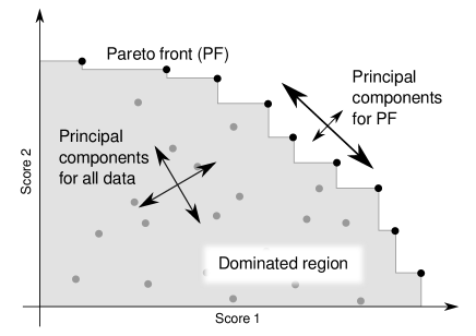
Figure 2: Schematic of the PCA with the PF. The arrows in the figure describe the PCs of the data and the variance of the data along the axes.

Correlation analysis follows collection of information about the PF (the optimizer-simulator loop) (Fig. 1). We use the results from the exhaustive simulation and show the data as a parallel coordinate plot for the target variables in the PF in Fig. 3 to visualize the correlation among the target variables. In the figure, a line denotes a system and links its target values on the parallel coordinates. There is a strong correlation between the magnetization and Curie temperature, which is shown as sharp diagonal line bunches between the $M_{\mathrm{s}}$ (magnetization) and $T_{\mathrm{C}}$ (Curie temperature) axes. In contrast, the price index has a weaker correlation with the magnetization and Curie temperature. Thus, the price can be reduced greatly by accepting a small reduction in the magnetization and Curie temperature.

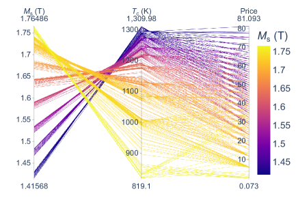
Figure 3: Parallel coordinate plot for the PF. The $M_{\mathrm{s}}$ axis shows the magnetization, the $T_{\mathrm{C}}$ axis shows the Curie temperature, and the Price axis shows the price index.

PCA can decompose these correlations into independent linear combinations of the variables by calculating the principal axes of the estimated covariance. Figure 4 shows the components of the principal axes, called principal components (PCs) with respect to the PF (bottom panels).

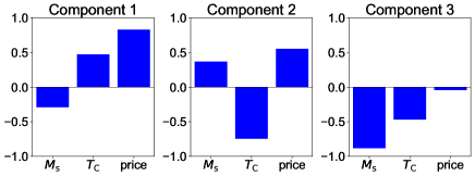
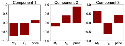
Figure 4: PC1, PC2, and PC3 (left to right) of the target variables for (top) the PF and (bottom) all data.

We also show the PCs for all data for comparison.

Because we consider three target variables, there are three principal axes. We call them PC1, PC2, and PC3 in descending order of variance along the axes. The directions of axes are different for the PF and all data. If PCs explain a large part of the variance in the PF (i.e., if the PFs have large variances along the PC) the PCs represent the trade-off among the target variables (Fig. 2). Because PC1 for the PF explains 57% of the variance and PC2 for the PF explains 40%, these two PCs are important.

The trade-offs can be summarized as follows. PC1 has positive components in the Curie temperature and price, and an opposite component in magnetization. Therefore, the Curie temperature increases at the cost of price and magnetization along the axis. Similarly, along PC2, the magnetization increases at the cost of price and Curie temperature. Both these PCs show a trade-off between the magnetization and Curie temperature; however, the price index has opposite correlations with them. This is how the weak correlation seen in Fig. 3 appears in the PCA.

This result is not obtained from the the PCA for all data, where PC1, which explains 90% of the variance in all data, is almost orthogonal to PC1 and PC2 for the PF. The PF can be used to see the trade-offs between the target variables clearly. The PCs for the PF resemble those for all data; PC1 for PF is similar to PC2 for all data, PC2 for PF is similar to PC3 for all data, and PC3 for PF is similar to PC1 for all data, although the order of the PCs are different. From this observation, we see that PC1 for all data indicates the direction that traverses the dominated region, and after filtering the non-PF members, the variance along the direction is greatly reduced, which is almost identical to PC3 for the PF.

We now consider controlling the target variables by changing the input variable as an example of the control variable analysis in Fig. 1. To analyze the descriptors, the simple application of PCA is not meaningful in our case because they are controllable variables and determined by an artificial choice; we choose the candidate systems so that they are distributed homogeneously in the descriptor space. We instead use the PLS2 regression, which searches the linear vector (X-weight) in the descriptor space that has the largest covariance with a vector in the target space (Y-weight) Holcomb et al. (1997). Let $C$ denote the cross-covariance matrix whose component is $C_{ij}=\sum_{d}(x^{(d)}_{i}-\bar{x}_{i})(y^{(d)}_{j}-\bar{y}_{j})$, where $x^{(d)}_{i}$ denotes the $d$th data for the $i$th input variable, $y^{(d)}_{j}$ denotes the $d$th data for the $j$th output variable, and the bar denotes the mean of the variable. (Division by a constant is omitted here because it does not change the result). Then, the singular value decomposition gives the decomposition,

$$C=\begin{pmatrix}{\vec{u}}_{1}&\cdots&{\vec{u}}_{M}\end{pmatrix}\begin{pmatrix}\lambda_{1}&&\\ &\ddots&\\ &&\lambda_{N}\\ &\text{\huge 0}\end{pmatrix}\begin{pmatrix}{}^{t}{\vec{v}}_{1}\\ \vdots\\ \vdots\\ {}^{t}{\vec{v}}_{N}\\ \end{pmatrix},$$ (4)

where $M$ is the input dimension, $N$ is the output dimension, ${\vec{u}}$ and ${\vec{v}}$ are sets of normalized orthonormal bases, and the diagonal $\lambda$ elements hold $\lambda_{1}\geq\cdots\geq\lambda_{N}$. We also assume that $M\geq N$ here for simplicity. The first X-weight vector is required to be proportional to ${\vec{u}}_{1}$, and the first Y-weight vector is determined by a linear regression of the data with respect to the values called X-score that are obtained by projecting the input data to the X-weight axis Holcomb et al. (1997).

In the next step, both the descriptor and target variable space are reduced by projection to the orthogonal complement of the the X- and Y-weight subspace. For the covariance, $C^{\prime}$, of reduced data, the second X- and Y-weights are determined in the same manner as the first. This is iterated until one of the spaces is reduced to zero dimensions.

The Y-weights are not necessarily identical to the results of the ordinary PCA. However, a similar set of Y-weights are obtained in our case, as shown in the bottom panels of Fig. 5. The corresponding X-weights are shown in the top panels, where we use the atomic numbers of $R$ ($Z_{R}$) and $Z$ ($Z_{Z}$), and the concentrations of Co ($\alpha_{\mathrm{Co}}$), $Z$ ($\alpha_{\mathrm{Z}}$), and Ti ($\alpha_{\mathrm{Ti}}$) as descriptor (explanatory) variables. This choice of descriptors is based on our previous study, in which we referred to this type of descriptor as #9 Fukazawa et al. (2019b).

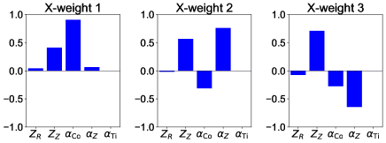
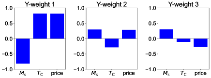
Figure 5: PLS for the PF. Weights for the (top) descriptor and (bottom) target variables.

The first Y-weight is similar to PC1 for PF in Fig. 4, and the corresponding X-weight has a large weight for Co (Fig. 5). The analysis rediscovers the efficiency of Co in enhancing the Curie temperature, which is already well-known, with the sacrifice of magnetization and cost. Because none of the PF systems contain Ti, the weight for Ti is zero for all components in Fig. 5.

The second Y-weight is similar to PC1 for the PF in Fig. 4, which represents a direction toward the increase in magnetization at the cost of the price and Curie temperature. The corresponding X-weight describes the choice of Dy as the $Z$ element, the increase of the $Z$ element, and the reduction of Co. Although the enhancement of magnetization by the reduction of Co is foreseeable, the contribution of Dy to magnetization is unexpected.

To see the validity of the PLS regression, we predict the magnetization, Curie temperature, and price index with the data projected to the X and Y-weight axes, and compare the standardized values of them with the actual values in Fig. 6. The coefficient of determination is 0.947, which shows the validity of the linear model for describing the distribution in the PF.

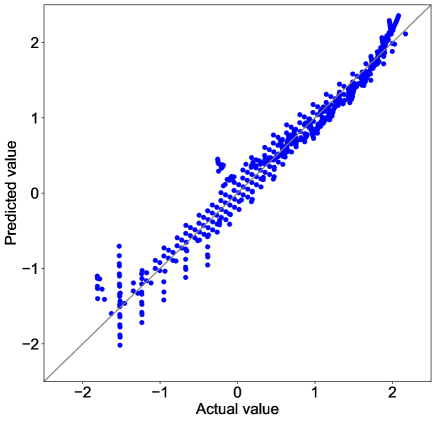
Figure 6: Actual versus predicted values with the PLS2 regression.

III.2 MBO

Although the analysis using the PF is powerful, obtaining the PF can be a difficult; in the present case, the PF consists of 253 members from the 3630 data points. First, we see how MBO is efficient in finding these true PF members. Because the MBO process uses a stochastic process, we need a statistical analysis in the performance evaluation. Figure 7 shows the number of true PF members found in the MBO search to determine how efficient MBO is.

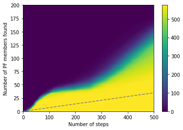
Figure 7: Step number versus number of true PF members found with MBO. The color map shows the frequency of obtaining a score higher than the vertical value in 575 sessions. The dashed line shows the analytic results with random sampling.

The color map in the figure shows the frequency of sessions that obtained a score higher than the value on the vertical axis within the number of steps indicated on the horizontal axis. The dashed line shows the mean score for random sampling. Although the MBO search is much more efficient than random sampling, it cannot find all the 253 PF members within 500 steps.

However, a tentative PF from the MBO session can serve as an approximated PF, from which the features of the true PF can be understood. To examine the validity of the approximated PFs, we construct a model for the target variables from tentative PFs with PLS2, and see how the model describes the true PF in terms of coefficient of determination.

Figure 8 shows the frequency of the sessions that obtained a coefficient of determination value larger than the value on the vertical axis within the steps indicated on the horizontal axis. In this case, 400 steps seems sufficient to generate a model that describes the features of the true PF when the number of the true PF members is 253. Therefore, this MBO scheme seems efficient in obtaining an approximate PF that can represent the true PF behaviors.

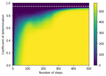
Figure 8: Step number versus the coefficient of determination (COD) with PLS2. The color map shows the frequency of obtaining a COD value higher than the vertical value in 575 sessions. The dashed line shows the COD value (0.947) with the true PF.

IV Conclusion

We proposed a scheme for analyzing the multi-objective correlation and the trade-offs among the target variables (Fig. 1). To determine the usefulness of the analyzer part of the framework, we performed PCA and PLS analysis for magnet compounds (R_$1-\alpha$$Z$_$\alpha$) (Fe_$1-\beta$Co_$\beta$)_$12-\gamma$Ti_$\gamma$ to extract information for searching for PF materials from first-principles data. The variance along the PF was characterized by PC1, which was controlled mainly by the introduction of Co, and by PC2, which was controlled mainly by simultaneous introduction of Dy and reduction of Co.

To demonstrate the efficiency of the scheme for obtaining an approximate PF, which is described as a loop before the analysis in Fig. 1, we conducted a performance evaluation with MBO. We showed that MBO obtained PF members much more efficiently than random sampling, and generated an approximate PF that adequately represented the true PF. We showed that a model could be constructed that described the true PF well from an approximate PF obtained with 400 first-principles calculations, where all the candidates consisted of 3630 systems.

References

- Ohashi et al. (1988a) K. Ohashi, Y. Tawara, R. Osugi, J. Sakurai, and Y. Komura, Journal of the Less Common Metals 139, L1 (1988a).
- Ohashi et al. (1988b) K. Ohashi, Y. Tawara, R. Osugi, and M. Shimao, J. Appl. Phys. 64, 5714 (1988b).
- Yang et al. (1988) Y.-c. Yang, L.-s. Kong, S.-h. Sun, D.-m. Gu, and B.-p. Cheng, Journal of applied physics 63, 3702 (1988).
- Verhoef et al. (1988) R. Verhoef, F. De Boer, Z. Zhi-dong, and K. Buschow, Journal of Magnetism and Magnetic Materials 75, 319 (1988).
- De Mooij and Buschow (1988) D. De Mooij and K. Buschow, Journal of the Less Common Metals 136, 207 (1988).
- Buschow (1988) K. Buschow, Journal of applied physics 63, 3130 (1988).
- Jaswal et al. (1990) S. S. Jaswal, Y. G. Ren, and D. J. Sellmyer, J. Appl. Phys. 67, 4564 (1990).
- Coehoorn (1990) R. Coehoorn, Phys. Rev. B 41, 11790 (1990).
- Buschow (1991) K. Buschow, Journal of magnetism and magnetic materials 100, 79 (1991).
- Sakurada et al. (1992) S. Sakurada, A. Tsutai, and M. Sahashi, Journal of Alloys and Compounds 187, 67 (1992).
- Sakuma (1992) A. Sakuma, J. Phys. Soc. Jpn. 61, 4119 (1992).
- Asano et al. (1993) S. Asano, S. Ishida, and S. Fujii, Physica B: Condensed Matter 190, 155 (1993).
- Akayama et al. (1994) M. Akayama, H. Fujii, K. Yamamoto, and K. Tatami, J. Magn. Magn. Mater. 130, 99 (1994).
- Kuz’min et al. (1999) M. D. Kuz’min, M. Richter, and K. H. J. Buschow, Solid State Commun. 113, 47 (1999).
- Gabay et al. (2016) A. M. Gabay, A. Martín-Cid, J. M. Barandiaran, D. Salazar, and G. C. Hadjipanayis, AIP Advances 6, 056015 (2016), https://doi.org/10.1063/1.4944066 .
- Körner et al. (2016) W. Körner, G. Krugel, and C. Elsässer, Scientific Reports 6, 24686 (2016).
- Ke and Johnson (2016) L. Ke and D. D. Johnson, Phys. Rev. B 94, 024423 (2016).
- Fukazawa et al. (2017) T. Fukazawa, H. Akai, Y. Harashima, and T. Miyake, Journal of Applied Physics 122, 053901 (2017).
- Fukazawa et al. (2019a) T. Fukazawa, H. Akai, Y. Harashima, and T. Miyake, Journal of Magnetism and Magnetic Materials 469, 296 (2019a).
- Hirayama et al. (2015a) Y. Hirayama, Y. Takahashi, S. Hirosawa, and K. Hono, Scripta Materialia 95, 70 (2015a).
- Hirayama et al. (2015b) Y. Hirayama, T. Miyake, and K. Hono, JOM 67, 1344 (2015b).
- Ohashi et al. (1987) K. Ohashi, T. Yokoyama, R. Osugi, and Y. Tawara, IEEE transactions on magnetics 23, 3101 (1987).
- Suzuki et al. (2014) S. Suzuki, T. Kuno, K. Urushibata, K. Kobayashi, N. Sakuma, K. Washio, H. Kishimoto, A. Kato, and A. Manabe, AIP Adv. 4, 117131 (2014).
- Sakuma et al. (2016) N. Sakuma, S. Suzuki, T. Kuno, K. Urushibata, K. Kobayashi, M. Yano, A. Kato, and A. Manabe, AIP Adv. 6, 056023 (2016).
- Kuno et al. (2016) T. Kuno, S. Suzuki, K. Urushibata, K. Kobayashi, N. Sakuma, M. Yano, A. Kato, and A. Manabe, AIP Adv. 6, 025221 (2016).
- Suzuki (2017) H. Suzuki, AIP Advances 7, 056208 (2017), https://doi.org/10.1063/1.4973799 .
- Harashima et al. (2016) Y. Harashima, K. Terakura, H. Kino, S. Ishibashi, and T. Miyake, Journal of Applied Physics 120, 203904 (2016).
- Fukazawa et al. (2021) T. Fukazawa, Y. Harashima, and T. Miyake, “First-principles study on the stability of (, zr)(fe, co, ti)12 against 2-17 and unary phases ( = y, nd, sm),” (2021), arXiv:2112.09297 [cond-mat.mtrl-sci] .
- Harashima et al. (2018) Y. Harashima, T. Fukazawa, H. Kino, and T. Miyake, Journal of Applied Physics 124, 163902 (2018).
- Ueno et al. (2016) T. Ueno, T. D. Rhone, Z. Hou, T. Mizoguchi, and K. Tsuda, Materials discovery 4, 18 (2016).
- Ju et al. (2017) S. Ju, T. Shiga, L. Feng, Z. Hou, K. Tsuda, and J. Shiomi, Physical Review X 7, 021024 (2017).
- Kikuchi et al. (2018) S. Kikuchi, H. Oda, S. Kiyohara, and T. Mizoguchi, Physica B: Condensed Matter 532, 24 (2018).
- Yuan et al. (2018) R. Yuan, Z. Liu, P. V. Balachandran, D. Xue, Y. Zhou, X. Ding, J. Sun, D. Xue, and T. Lookman, Advanced Materials 30, 1702884 (2018).
- Fukazawa et al. (2019b) T. Fukazawa, Y. Harashima, Z. Hou, and T. Miyake, Physical Review Materials 3, 053807 (2019b).
- Fukazawa et al. (2022) T. Fukazawa, H. Akai, Y. Harashima, and T. Miyake, Acta Materialia 226, 117597 (2022).
- Hohenberg and Kohn (1964) P. Hohenberg and W. Kohn, Physical Review 136, B864 (1964).
- Kohn and Sham (1965) W. Kohn and L. J. Sham, Physical Review 140, A1133 (1965).
- Korringa (1947) J. Korringa, Physica 13, 392 (1947).
- Kohn and Rostoker (1954) W. Kohn and N. Rostoker, Phys. Rev. 94, 1111 (1954).
- Jensen and Mackintosh (1991) J. Jensen and A. R. Mackintosh, Rare earth magnetism (Clarendon Oxford, 1991).
- Locht et al. (2016) I. L. M. Locht, Y. O. Kvashnin, D. C. M. Rodrigues, M. Pereiro, A. Bergman, L. Bergqvist, A. I. Lichtenstein, M. I. Katsnelson, A. Delin, A. B. Klautau, B. Johansson, I. Di Marco, and O. Eriksson, Phys. Rev. B 94, 085137 (2016).
- Richter (1998) M. Richter, Journal of Physics D: Applied Physics 31, 1017 (1998).
- Perdew and Zunger (1981) J. P. Perdew and A. Zunger, Phys. Rev. B 23, 5048 (1981).
- Soven (1970) P. Soven, Physical Review B 2, 4715 (1970).
- Shiba (1971) H. Shiba, Progress of Theoretical Physics 46, 77 (1971).
- Liechtenstein et al. (1987) A. I. Liechtenstein, M. Katsnelson, V. Antropov, and V. Gubanov, Journal of Magnetism and Magnetic Materials 67, 65 (1987).
- Pedregosa et al. (2011) F. Pedregosa, G. Varoquaux, A. Gramfort, V. Michel, B. Thirion, O. Grisel, M. Blondel, P. Prettenhofer, R. Weiss, V. Dubourg, et al., Journal of machine learning research 12, 2825 (2011).
- Wold et al. (1987) S. Wold, K. Esbensen, and P. Geladi, Chemometrics and intelligent laboratory systems 2, 37 (1987).
- Holcomb et al. (1997) T. R. Holcomb, H. Hjalmarsson, M. Morari, and M. L. Tyler, Journal of Chemometrics: A Journal of the Chemometrics Society 11, 283 (1997).
- (50) “PHYSBO – optimization tools for PHYsics based on Bayesian Optimization,” https://github.com/issp-center-dev/PHYSBO.
- Motoyama et al. (2022) Y. Motoyama, R. Tamura, K. Yoshimi, K. Terayama, T. Ueno, and K. Tsuda, Computer Physics Communications 278, 108405 (2022).
- Couckuyt et al. (2014) I. Couckuyt, D. Deschrijver, and T. Dhaene, Journal of Global Optimization 60, 575 (2014).