Joint distribution of two Local Times for diffusion processes
with the application to the construction of various conditioned processes

Abstract

For a diffusion process $X(t)$ of drift $\mu(x)$ and of diffusion coefficient $D=1/2$, we study the joint distribution of the two local times $A(t)=\int_{0}^{t}d\tau\delta(X(\tau))$ and $B(t)=\int_{0}^{t}d\tau\delta(X(\tau)-L)$ at positions $x=0$ and $x=L$, as well as the simpler statistics of their sum $\Sigma(t)=A(t)+B(t)$. Their asymptotic statistics for large time $t\to+\infty$ involves two very different cases : (i) when the diffusion process $X(t)$ is transient, the two local times $[A(t);B(t)]$ remain finite random variables $[A^{*}(\infty),B^{*}(\infty)]$ and we analyze their limiting joint distribution ; (ii) when the diffusion process $X(t)$ is recurrent, we describe the large deviations properties of the two intensive local times $a=\frac{A(t)}{t}$ and $b=\frac{B(t)}{t}$ and of their intensive sum $\sigma=\frac{\Sigma(t)}{t}=a+b$. These properties are then used to construct various conditioned processes $[X^{*}(t),A^{*}(t),B^{*}(t)]$ satisfying certain constraints involving the two local times, thereby generalizing our previous work [J. Stat. Mech. (2022) 103207] concerning the conditioning with respect to a single local time $A(t)$. In particular for the infinite time horizon $T\to+\infty$, we consider the conditioning towards the finite asymptotic values $[A^{*}(\infty),B^{*}(\infty)]$ or $\Sigma^{*}(\infty)$, as well as the conditioning towards the intensive values $[a^{*},b^{*}]$ or $\sigma^{*}$, that can be compared with the appropriate ’canonical conditioning’ based on the generating function of the local times in the regime of large deviations. This general construction is then applied to the simplest case where the unconditioned diffusion is the Brownian motion of uniform drift $\mu$.

I Introduction

I.1 Local Times as the basic time-additive observables for diffusion processes

For a one-dimensional diffusion process $X(t)$, two essential time-additive observables of the stochastic trajectory $X(0\leq\tau\leq t)$ are :

(i) the occupation time $O_{[x_{L},x_{R}]}(t)$ of the space interval $[x_{L},x_{R}]$ during the time window $[0,t]$

$$O_{[x_{L},x_{R}]}(t)=\int_{0}^{t}d\tau\theta(x_{L}\leq X(\tau)\leq x_{R})$$ (1)

that belongs to the interval $0\leq O_{[x_{L},x_{R}]}(t)\leq t$.

(ii) the local time $A_{x}(t)$ at the position $x$ during the time window $[0,t]$ (see the mathematical review [1] and references therein)

$$A_{x}(t)=\int_{0}^{t}d\tau\delta(X(\tau)-x)$$ (2)

that has for physical dimension $\frac{Time}{Length}$ (in contrast to the physical dimension Time for Eq. 1) and that belongs to $[0,+\infty[$ with no upper bound. The direct links with the occupation times of Eq. 1 can be summarized as follows. On one hand, the local time $A_{x}(t)$ of Eq. 2 can be constructed from the occupation time $O_{[x-\epsilon,x+\epsilon]}(t)$ of the space interval $[x-\epsilon,x+\epsilon]$ of size $(2\epsilon)>0$ centered at the position $x$ in the limit $\epsilon\to 0^{+}$

$$A_{x}(t)=\int_{0}^{t}d\tau\mathop{\lim}_{\epsilon\to 0^{+}}\left(\frac{\theta(x-\epsilon\leq X(\tau)\leq x+\epsilon)}{2\epsilon}\right)=\mathop{\lim}_{\epsilon\to 0^{+}}\left(\frac{O_{[x-\epsilon,x+\epsilon]}(t)}{2\epsilon}\right)$$ (3)

On the other hand, the occupation time $O_{[x_{L},x_{R}]}(t)$ can be reconstructed from the local time $A_{x}(t)$ for all the internal positions $x\in[x_{L},x_{R}]$

$$O_{[x_{L},x_{R}]}(t)=\int_{0}^{t}d\tau\int_{x_{L}}^{x_{R}}dx\delta(X(\tau)-x)=\int_{x_{L}}^{x_{R}}dxA_{x}(t)$$ (4)

As a consequence, both the occupation times and the local times have attracted a lot of interest recently in the physics literature for many different contexts (see [2, 3, 4, 5, 6, 7, 8, 9, 10, 11, 12, 13, 14, 15] and references therein).

More generally, the local times $A_{x}(t)$ of Eq. 2 allow to reconstruct any time-additive observable involving an arbitrary function $f(.)$

$$\int_{0}^{t}d\tau f(X(\tau))=\int_{-\infty}^{+\infty}dxf(x)A_{x}(t)$$ (5)

and can be thus considered as the basic time-additive observables. Time-additive observables like Eq. 5 are of course interesting for their own statistical properties, but they can also be used to construct conditioned processes as we now recall.

I.2 Reminder on the conditioning of stochastic processes with respect to time-additive observables

Since its introduction by Doob [17, 18], the conditioning of stochastic processes (see the mathematical books [19, 20, 21] and the physics recent review [22]) have found many applications in various fields like ecology [23], finance [24] or nuclear engineering [25, 26]. Over the years, many different conditioning constraints have been considered, including the Brownian excursion [27, 28], the Brownian meander [29], the taboo processes [30, 31, 32, 33, 34, 35], or non-intersecting Brownian bridges [36]. Let us also mention the conditioning in the presence of killing rates [19, 37, 38, 39, 40, 41, 42, 43, 44] or when the killing occurs only via an absorbing boundary condition [45, 46, 47, 48]. Stochastic bridges have been also studied for many other Markov processes, including various diffusions processes [49, 50, 51], discrete-time random walks and Lévy flights [52, 53, 54], continuous-time Markov jump processes [54], run-and-tumble trajectories [55], or processes with resetting [56].

For the present work, the recent important generalization concerns the conditioning with respect to global dynamical constraints involving time-additive observables of the stochastic trajectories. In particular, the conditioning on the area has been studied via various methods for Brownian processes or bridges [57] and for Ornstein-Uhlenbeck bridges [58]. The conditioning on the area and on other time-additive observables has been then analyzed both for the Brownian motion and for discrete-time random walks [59]. This approach has been generalized [60] to various types of discrete-time or continuous-time Markov processes, while the time-additive observable can involve both the time spent in each configuration and the increments of the Markov process. This general reformulation of the ’microcanonical conditioning’, where the time-additive observable is constrained to reach a given value after the finite time window $T$, allows to make the link [60] with the ’canonical conditioning’ based on generating functions of additive observables that has been much studied recently in the field of dynamical large deviations of Markov processes over a large time-window $T$ [61, 62, 63, 64, 65, 66, 67, 68, 69, 70, 71, 72, 73, 74, 75, 76, 77, 78, 79, 80, 81, 82, 83, 84, 85, 86, 87, 88, 89, 90, 94, 95, 96, 91, 92, 93, 97, 98, 99, 100, 101, 102, 103, 104, 105, 106]. The equivalence between the ’microcanonical conditioning’ and the ’canonical conditioning’ at the level of the large deviations for large time $T$ is explained in detail in the two complementary papers [84, 85] and in the HDR thesis [86].

I.3 Goals and organization of the present paper

As recalled in the previous subsection, the methods to construct conditioned processes with respect to time-additive observables are now well-established, both in the ’microcanonical’ and in the ’canonical’ perspectives. However, the concrete application to specific time-additive observables like Eq. 5 for given Markov processes remains often challenging. It is thus important to identify the cases where conditioned processes can be explicitly constructed and what level of technicality is required to perform the computations.

At first sight, the delta function that enters the definition of the local time in Eq. 2 might appear as very singular. However, as in quantum mechanics where delta impurities are well-known to be much simpler than smoother potentials, the delta function in Eq. 2 is actually a huge technical simplification with respect to the arbitrary general additive observable of Eq. 5. Indeed, the exact Dyson equation associated to a single delta impurity allows to analyze the statistics of a single local time in terms of the properties of the propagator $G_{t}(x|x_{0})$ of the diffusion process $X(t)$ alone, as recalled in detail in [16]. In the present paper, it will be thus interesting to use similarly the exact Dyson equation associated to two single delta impurities in order to characterize the joint statistics of the two Local Times $A(t)=A_{x=0}(t)$ and $B(t)=A_{x=L}(t)$ at positions $x=0$ and $x=L$

$$A(t) \equiv\int_{0}^{t}d\tau\delta(X(\tau))$$

$$B(t) \equiv\int_{0}^{t}d\tau\delta(X(\tau)-L)$$ (6)

for a diffusion process $X(t)$ of diffusion coefficient $D=1/2$ with an arbitrary position-dependent drift $\mu(x)$, thereby generalizing the explicit joint statistics of the two local boundary times for the Brownian motion with no drift $\mu(x)=0$ on the interval $[0,L]$ with reflecting boundary conditions at $x=0$ and $x=L$ computed recently [6]. The paper is organized as follows.

In section II, we focus on the joint dynamics of the position $X(t)$ and of the two local times $A(t)$ and $B(t)$ of Eq. 6 satisfying the Ito Stochastic Differential System involving the Wiener process $W(t)$

$$dX(t) =\mu(X(t))dt+dW(t)$$

$$dA(t) =\delta(X(t))dt$$

$$dB(t) =\delta(X(t)-L)dt$$ (7)

We use the Feynman-Kac formula and the Dyson equation in order to compute explicitly the time-Laplace-transform of parameter $s$ of the joint distribution $P_{t}(x,A,B|x_{0})$ to see $[X(t)=x;A(t)=A,B(t)=B$ when starting at $[X(0)=x_{0};A(0)=0;B(0)=0]$

$${\hat{P}}_{s}(x,A,B|x_{0})\equiv\int_{0}^{+\infty}dte^{-st}P_{t}(x,A,B|x_{0})$$ (8)

In section III, we focus on the joint distribution $\Pi_{t}(A,B|x_{0})$ of the two local times $[X(t)=x;A(t)=A,B(t)=B$ at time $t$ when starting at $[X(0)=x_{0};A(0)=0;B(0)=0]$

$$\Pi_{t}(A,B|x_{0})\equiv\int_{-\infty}^{+\infty}dxP_{t}(x,A,B|x_{0})$$ (9)

and we compute explicitly the time-Laplace-transform of parameter $s$

$${\hat{\Pi}}_{s}(A,B|x_{0}) \equiv\int_{0}^{+\infty}dte^{-st}\Pi_{t}(A,B|x_{0})=\int_{-\infty}^{+\infty}dx{\hat{P}}_{s}(x,A,B|x_{0})$$ (10)

In section IV, we analyse the behavior for large time $t$ of the joint distribution $\Pi_{t}(A,B|x_{0})$. When the diffusion process $X(t)$ is transient, the two local times $(A,B)$ remain finite random variables for $t\to+\infty$ and we compute the limit joint distribution $\Pi_{\infty}(A,B|x_{0})$. When the diffusion process $X(t)$ is recurrent, then it is more appropriate to introduce the two intensive local times

$$a \equiv\frac{A}{t}$$

$$b \equiv\frac{B}{t}$$ (11)

and to analyze their joint large deviations properties

$$\Pi_{t}(A=ta,B=tb|x_{0}) \mathop{\simeq}_{t\to+\infty}\aleph_{t}(a,b,x_{0})e^{-tI(a,b)}$$ (12)

where the positive rate function $I(a,b)\geq 0$ governs the leading exponential decay in time, while the prefactor $\aleph_{t}(a,b,x_{0})$ that contains the dependence with respect to the initial position $x_{0}$ will be also computed explicitly. In section V, we describe the corresponding simpler statistical properties of the sum $\Sigma(t)=A(t)+B(t)$ of the two local times.

In section VI, we construct various conditioned joint processes $[X^{*}(t),A^{*}(t),B^{*}(t)]$ satisfying certain constraints involving the two local times, thereby generalizing our previous work [16] concerning the conditioning with respect to the single local time $A(t)$. The conditioned Bridge towards the given local times $[A^{*}_{T},B^{*}_{T}]$ at the finite time horizon $T$ can be constructed as follows : the conditioned process $[X^{*}(t),A^{*}(t),B^{*}(t)]$ satisfies the following Ito SDE system analog to Eq. 7

$$dX^{*}(t) =\mu^{[A_{T}^{*},B_{T}^{*}]}_{T}(X^{*}(t),A^{*}(t),B^{*}(t),t)dt+dW(t)$$

$$dA^{*}(t) =\delta(X^{*}(t))dt$$

$$dB^{*}(t) =\delta(X^{*}(t)-L)dt$$ (13)

where the conditioned drift $\mu^{[A_{T}^{*},B_{T}^{*}]}_{T}(x,A,B,t)$ involves the unconditioned drift $\mu(x)$ and the logarithmic derivative of the unconditioned distribution $\Pi_{T-t}(A_{T}^{*}-A,B_{T}^{*}-B|x)$ with respect to its initial position $x$

$$\mu^{[A_{T}^{*},B_{T}^{*}]}_{T}(x,A,B,t)=\mu(x)+\partial_{x}\ln\Pi_{T-t}(A_{T}^{*}-A,B_{T}^{*}-B|x)$$ (14)

In the limit of the infinite time horizon $T\to+\infty$, we will analyze the conditioning towards the finite asymptotic values $[A^{*}(\infty),B^{*}(\infty)]$, as well as the conditioning towards the intensive values $[a^{*},b^{*}]$.

In section VII, the general framework of the previous sections written for the diffusion process with an arbitrary unconditioned drift $\mu(x)$ is applied to the simplest example of the Brownian motion with the uniform drift $\mu(x)=\mu$ on the whole line $]-\infty,+\infty[$ in order to construct various conditioned processes involving its two local times. Our conclusions are summarized in section VIII. The two appendices A and B are devoted to the canonical conditioned processes $X^{*}_{p,q}(t)$ of parameters $(p,q)$ conjugated to the two local times $A$ and $B$, in order to compare with the microcanonical conditioning described in the main text. Two other Appendices C D contain more technical computations.

II Propagator $P_{t}(x,A,B|x_{0})$ for the position $x$ and the two local times $A$ and $B$

In this section, we analyze the joint propagator $P_{t}(x,A,B|x_{0})$ associated to the Ito system of Eq. 7 that satisfies the Fokker-Planck dynamics

$$\partial_{t}P_{t}(x,A,B|x_{0})=-\delta(x)\partial_{A}P_{t}(x,A,B|x_{0})-\delta(x-L)\partial_{B}P_{t}(x,A,B|x_{0})-\partial_{x}\left[\mu(x)P_{t}(x,A,B|x_{0})\right]+\frac{1}{2}\partial_{x}^{2}P_{t}(x,A,B|x_{0})\ \ \ \ \ \$$ (15)

For clarity, it will be convenient to denote by another letter the propagator $G_{t}(x|x_{0})$ of the position $x$ alone

$$G_{t}(x|x_{0})=\int_{0}^{+\infty}dA\int_{0}^{+\infty}dBP_{t}(x,A,B|x_{0})$$ (16)

that satisfies

$$\partial_{t}G_{t}(x|x_{0})=-\partial_{x}\left[\mu(x)G_{t}(x|x_{0})\right]+\frac{1}{2}\partial_{x}^{2}G_{t}(x|x_{0})$$ (17)

II.1 Decomposition of the joint propagator $P_{t}(x,A,B|x_{0})$ into four contributions

The joint propagator $P_{t}(x,A,B|x_{0})$ can be decomposed into the four contributions based on the two delta functions $\delta(A)$ and $\delta(B)$ and on the two Heaviside functions $\theta(A>0)$ and $\theta(B>0)$

$$P_{t}(x,A,B|x_{0}) =\delta(A)\delta(B)G^{abs(0,L)}_{t}(x|x_{0})+\theta(A>0)\delta(B){\cal A}^{abs(L)}_{t}(x,A|x_{0})+\delta(A)\theta(B>0){\cal B}^{abs(0)}_{t}(x,B|x_{0})$$ (18)

$$+\theta(A>0)\theta(B>0){\cal C}_{t}(x,A,B|x_{0})$$

with the following meaning.

(1) The first contribution containing the two delta functions $\delta(A)\delta(B)$ means that the two local times have kept their initial values $A=0$ and $B=0$, i.e. the diffusion process has not been able to visit the positions $x=0$ and $x=L$. As a consequence, the amplitude is given by the propagator $G^{abs(0,L)}_{t}(x|x_{0})$ in the presence of two absorbing boundary conditions at position $0$ and at position $L$, so that it is non-vanishing only if the the final position $x$ and the initial position $x_{0}$ belong both to the left region $]-\infty,0[$, or belong both to the middle region $]0,L[$ or belong both to the right region $]L,+\infty[$, and in the two external regions, only one absorbing boundary condition is sufficient

$$G^{abs(0,L)}_{t}(x|x_{0}) =\theta(x<0)\theta(x_{0}<0)G^{abs(0)}_{t}(x|x_{0})$$ (19)

$$+\theta(0<x<L)\theta(0<x_{0}<L)G^{abs(0,L)}_{t}(x|x_{0})$$

$$+\theta(x>L)\theta(x_{0}>L)G^{abs(L)}_{t}(x|x_{0})$$

(2) The second contribution containing $\theta(A>0)\delta(B)$ means that the diffusion process has not been able to visit $x=L$ but has visited $x=0$, so that it is non-vanishing only for $x<L$ and $x_{0}<L$

$${\cal A}^{abs(L)}_{t}(x,A|x_{0})=\theta(x<L)\theta(x_{0}<L){\cal A}^{abs(L)}_{t}(x,A|x_{0})$$ (20)

(3) The third contribution containing $\delta(A)\theta(B>0)$ means that the diffusion process has not been able to visit $x=0$ but has visited $x=L$, so that it is non-vanishing only for $x>0$ and $x_{0}>0$

$${\cal B}^{abs(0)}_{t}(x,B|x_{0})=\theta(x>0)\theta(x_{0}>0){\cal B}^{abs(0)}_{t}(x,B|x_{0})$$ (21)

(4) The fourth contribution containing $\theta(A>0)\theta(B>0)$ means that the diffusion process has visited both positions $x=0$ and $x=L$.

Figure 1 shows examples of trajectories of the Brownian bridge that illustrate these four contributions of the propagator $P_{t}(x,A,B|x_{0})$ in Eq. 18.

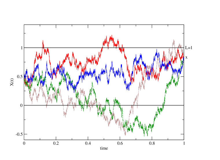
Figure 1: Examples of simulated trajectories $x(t)$ of the Brownian bridge on the interval $t\in[0,1]$ that illustrate the four contributions of the joint propagator $P_{t}(x,A,B|x_{0})$ in Eq. 18. The four trajectories $x(t)$ start from $x_{0}=0.5$ at time $t=0$ and end at $x=0.8$ at time $t=1$, but have different properties with respect to the two local times $A$ and $B$: the blue trajectory that has not been able to visit the position $x=0$ and $x=L=1$ contributes to the first term of Eq. 18 involving $\delta(A)\delta(B)$; the green trajectory that has not been able to visit $x=L=1$ but has visited $x=0$ contributes to the second term of Eq. 18 involving $\theta(A>0)\delta(B)$; the red trajectory that has not been able to visit $x=0$ but has visited $x=L=1$ contributes to the third term of Eq. 18 involving $\delta(A)\theta(B>0)$ ; the brown trajectory that has visited both positions $x=0$ and $x=L=1$ contributes to the fourth term of Eq. 18 involving $\theta(A>0)\theta(B>0)$. The time step used in the discretization is $dt=10^{-4}$

II.2 Laplace transform ${\tilde{P}}_{t,p,q}(x|x_{0})$ with respect to the two local times $A$ and $B$ : Feynman-Kac formula

For the Laplace transform ${\tilde{P}}_{t,p,q}(x|x_{0})$ of the propagator $P_{t}(x,A,B|x_{0})$ of Eq. 18 with respect to the two local times $A$ and $B$

$${\tilde{P}}_{t,p,q}(x|x_{0}) \equiv\int_{0}^{+\infty}dAe^{-pA}\int_{0}^{+\infty}dBe^{-qB}P_{t}(x,A,B|x_{0})$$ (22)

$$=G^{abs(0,L)}_{t}(x|x_{0})+{\tilde{\cal A}^{abs(L)}}_{t,p}(x|x_{0})+{\tilde{\cal B}}^{abs(0)}_{t,q}(x|x_{0})+{\tilde{\cal C}}_{t,p,q}(x|x_{0})$$

Eq. 15 translates into

$$\partial_{t}{\tilde{P}}_{t,p,q}(x|x_{0}) =-p\delta(x){\tilde{P}}_{t,p,q}(x|x_{0})-q\delta(x-L){\tilde{P}}_{t,p,q}(x|x_{0})-\partial_{x}\left[\mu(x){\tilde{P}}_{t,p,q}(x|x_{0})\right]+\frac{1}{2}\partial_{x}^{2}{\tilde{P}}_{t,p,q}(x|x_{0})$$ (23)

For $p=0=q$, one recovers the propagator $G_{t}(x|x_{0})$ of the position alone

$${\tilde{P}}_{t,p=0,q=0}(x|x_{0})=G_{t}(x|x_{0})$$ (24)

Eq. 23 is an example of the Feynman-Kac formula, where the initial Fokker-Planck dynamics of Eq. 17 is now supplemented by the two additional terms involving $p\delta(x)$ and $q\delta(x-L)$.

II.3 Explicit solution for the further time-Laplace-transform ${\hat{\tilde{P}}}_{s,p,q}(x|x_{0})$ via the Dyson Equation

For the further Laplace transform ${\hat{\tilde{P}}}_{s,p,q}(x|x_{0})$ of Eq. 22 with respect to the time $t$

$${\hat{\tilde{P}}}_{s,p,q}(x|x_{0}) \equiv\int_{0}^{+\infty}dte^{-st}{\tilde{P}}_{t,p,q}(x|x_{0})$$ (25)

$$={\hat{G}}^{abs(0,L)}_{s}(x|x_{0})+{\hat{\tilde{\cal A}}}^{abs(L)}_{s,p}(x|x_{0})+{\hat{\tilde{\cal B}}}^{abs(0)}_{s,q}(x|x_{0})+{\hat{\tilde{\cal C}}}_{s,p,q}(x|x_{0})$$

Eq. 23 translates into

$$-\delta(x-x_{0})+s{\hat{\tilde{P}}}_{s,p,q}(x|x_{0})=-p\delta(x){\hat{\tilde{P}}}_{s,p,q}(0|x_{0})-q\delta(x-L){\hat{\tilde{P}}}_{s,p,q}(L|x_{0})-\partial_{x}\left[\mu(x){\hat{\tilde{P}}}_{s,p,q}\right]+\frac{1}{2}\partial_{x}^{2}{\hat{\tilde{P}}}_{s,p,q}$$ (26)

The knowledge of the solution for $p=q=0$ of Eq. 24

$${\hat{\tilde{P}}}_{s,p=0,q=0}(x|x_{0})={\hat{G}}_{s}(x|x_{0})$$ (27)

allows to rewrite the solution for arbitrary Laplace parameters $(p,q)$ as

$${\hat{\tilde{P}}}_{s,p,q}(x|x_{0})={\hat{G}}_{s}(x|x_{0})-p{\hat{G}}_{s}(x|0){\hat{\tilde{P}}}_{s,p,q}(0|x_{0})-q{\hat{G}}_{s}(x|L){\hat{\tilde{P}}}_{s,p,q}(L|x_{0})$$ (28)

where ${\hat{\tilde{P}}}_{s,p,q}(0|x_{0})$ and ${\hat{\tilde{P}}}_{s,p,q}(L|x_{0})$ should satisfy the following system, where Eq. 28 is written for $x=0$ and for $x=L$ respectively

$$\left[1+p{\hat{G}}_{s}(0|0)\right]{\hat{\tilde{P}}}_{s,p,q}(0|x_{0})+q{\hat{G}}_{s}(0|L){\hat{\tilde{P}}}_{s,p,q}(L|x_{0}) ={\hat{G}}_{s}(0|x_{0})$$

$$p{\hat{G}}_{s}(L|0){\hat{\tilde{P}}}_{s,p,q}(0|x_{0})+\left[1+q{\hat{G}}_{s}(L|L)\right]{\hat{\tilde{P}}}_{s,p,q}(L|x_{0}) ={\hat{G}}_{s}(L|x_{0})$$ (29)

The solution of this system

$${\hat{\tilde{P}}}_{s,p,q}(0|x_{0}) =\frac{\left[1+q{\hat{G}}_{s}(L|L)\right]{\hat{G}}_{s}(0|x_{0})-q{\hat{G}}_{s}(0|L){\hat{G}}_{s}(L|x_{0})}{\left[1+p{\hat{G}}_{s}(0|0)\right]\left[1+q{\hat{G}}_{s}(L|L)\right]-pq{\hat{G}}_{s}(L|0){\hat{G}}_{s}(0|L)}$$

$${\hat{\tilde{P}}}_{s,p,q}(L|x_{0}) =\frac{\left[1+p{\hat{G}}_{s}(0|0)\right]{\hat{G}}_{s}(L|x_{0})-p{\hat{G}}_{s}(L|0){\hat{G}}_{s}(0|x_{0})}{\left[1+p{\hat{G}}_{s}(0|0)\right]\left[1+q{\hat{G}}_{s}(L|L)\right]-pq{\hat{G}}_{s}(L|0){\hat{G}}_{s}(0|L)}$$ (30)

can be plugged into Eq. 28 to obtain the general solution

$${\hat{\tilde{P}}}_{s,p,q}(x|x_{0}) ={\hat{G}}_{s}(x|x_{0})-\frac{pq\Omega_{s}(x|x_{0})+p\frac{{\hat{G}}_{s}(x|0){\hat{G}}_{s}(0|x_{0})}{\Delta_{s}}+q\frac{{\hat{G}}_{s}(x|L){\hat{G}}_{s}(L|x_{0})}{\Delta_{s}}}{pq+p\frac{{\hat{G}}_{s}(0|0)}{\Delta_{s}}+q\frac{{\hat{G}}_{s}(L|L)}{\Delta_{s}}+\frac{1}{\Delta_{s}}}$$ (31)

where we have introduced the two following notations

$$\Delta_{s} \equiv{\hat{G}}_{s}(0|0){\hat{G}}_{s}(L|L)-{\hat{G}}_{s}(L|0){\hat{G}}_{s}(0|L)$$ (32)

$$\Omega_{s}(x|x_{0}) \equiv\frac{{\hat{G}}_{s}(L|L){\hat{G}}_{s}(x|0){\hat{G}}_{s}(0|x_{0})-{\hat{G}}_{s}(x|0){\hat{G}}_{s}(0|L){\hat{G}}_{s}(L|x_{0})+{\hat{G}}_{s}(0|0){\hat{G}}_{s}(x|L){\hat{G}}_{s}(L|x_{0})-{\hat{G}}_{s}(x|L){\hat{G}}_{s}(L|0){\hat{G}}_{s}(0|x_{0})}{\Delta_{s}}$$

in order to see more clearly the rational fraction structure of Eq. 31 with respect to the two Laplace parameters $(p,q)$.

II.4 Explicit Laplace inversion of ${\hat{\tilde{P}}}_{s,p,q}(x|x_{0})$ with respect to $p$ and $q$ to obtain ${\hat{P}}_{s}(x,A,B|x_{0})$

The goal is now to obtain the time-Laplace-transform of parameter $s$ of the propagator of Eq. 18 with its four contributions

$${\hat{P}}_{s}(x,A,B|x_{0}) \equiv\int_{0}^{+\infty}dte^{-st}P_{t}(x,A,B|x_{0})$$ (33)

$$=\delta(A)\delta(B){\hat{G}}^{abs(0,L)}_{s}(x|x_{0})+\theta(A>0)\delta(B){\hat{\cal A}}^{abs(L)}_{s}(x,A|x_{0})+\delta(A)\theta(B>0){\hat{\cal B}}^{abs(0)}_{s}(x,B|x_{0})$$

$$+\theta(A>0)\theta(B>0){\hat{\cal C}}_{s}(x,A,B|x_{0})$$

from the Laplace inversion with respect to the two Laplace parameters $(p,q)$ of

$${\hat{\tilde{P}}}_{s,p,q}(x|x_{0}) =\int_{0}^{+\infty}dAe^{-pA}\int_{0}^{+\infty}dBe^{-qB}{\hat{P}}_{s}(x,A,B|x_{0})$$ (34)

$$={\hat{G}}^{abs(0,L)}_{s}(x|x_{0})+\int_{0}^{+\infty}dAe^{-pA}{\hat{\cal A}}^{abs(L)}_{s}(x,A|x_{0})+\int_{0}^{+\infty}dBe^{-qB}{\hat{\cal B}}^{abs(0)}_{s}(x,B|x_{0})$$

$$+\int_{0}^{+\infty}dAe^{-pA}\int_{0}^{+\infty}dBe^{-qB}{\hat{\cal C}}_{s}(x,A,B|x_{0})$$

$$={\hat{G}}^{abs(0,L)}_{s}(x|x_{0})+{\hat{\tilde{\cal A}}}^{abs(L)}_{s,p}(x|x_{0})+{\hat{\tilde{\cal B}}}^{abs(0)}_{s,q}(x|x_{0})+{\hat{\tilde{\cal C}}}_{s,p,q}(x|x_{0})$$

whose explicit expression was computed in Eq. 31.

II.4.1 First contribution of amplitude ${\hat{G}}^{abs(0,L)}_{s}(x|x_{0})$

Equation 34 yields that the first contribution ${\hat{G}}^{abs(0,L)}_{s}(x|x_{0})$ can be found by considering the double limit $(p\to+\infty,q\to+\infty)$ of ${\hat{\tilde{P}}}_{s,p,q}(x|x_{0})$ given by Eq. 31

$${\hat{G}}^{abs(0,L)}_{s}(x|x_{0})={\hat{\tilde{P}}}_{s,p=+\infty,q=+\infty}(x|x_{0})={\hat{G}}_{s}(x|x_{0})-\Omega_{s}(x|x_{0})$$ (35)

II.4.2 Second contribution of amplitude ${\hat{\cal A}}^{abs(L)}_{s}(x,A|x_{0})$

Equation 34 yields that the second contribution ${\hat{\tilde{\cal A}}}^{abs(L)}_{s,p}(x|x_{0})$ can be found by considering the limit $q\to+\infty$ of ${\hat{\tilde{P}}}_{s,p,q}(x|x_{0})$ given by Eq. 31

$${\hat{G}}^{abs(0,L)}_{s}(x|x_{0})+{\hat{\tilde{\cal A}}}^{abs(L)}_{s,p}(x|x_{0}) ={\hat{\tilde{P}}}_{s,p,q=+\infty}(x|x_{0})={\hat{G}}_{s}(x|x_{0})-\frac{p\Omega_{s}(x|x_{0})+\frac{{\hat{G}}_{s}(x|L){\hat{G}}_{s}(L|x_{0})}{\Delta_{s}}}{p+\frac{{\hat{G}}_{s}(L|L)}{\Delta_{s}}}$$ (36)

The difference with the first contribution of Eq. 35 yields

$${\hat{\tilde{\cal A}}}^{abs(L)}_{s,p}(x|x_{0})=\Omega_{s}(x|x_{0})-\frac{p\Omega_{s}(x|x_{0})+\frac{{\hat{G}}_{s}(x|L){\hat{G}}_{s}(L|x_{0})}{\Delta_{s}}}{p+\frac{{\hat{G}}_{s}(L|L)}{\Delta_{s}}}=\frac{\alpha_{s}^{[00]}(x|x_{0})}{p+\frac{1}{{\hat{G}}^{abs(L)}_{s}(0|0)}}$$ (37)

where we have introduced the Laplace transform ${\hat{G}}_{s}^{abs(L)}(x|x_{0})$ of the propagator $G^{abs(L)}_{t}(x|x_{0})$ in the presence of a single absorbing boundary at $x=L$

$${\hat{G}}_{s}^{abs(L)}(x|x_{0})\equiv\int_{0}^{+\infty}dte^{-st}G^{abs(L)}_{t}(x|x_{0})={\hat{G}}_{s}(x|x_{0})-\frac{{\hat{G}}_{s}(x|L){\hat{G}}_{s}(L|x_{0})}{{\hat{G}}_{s}(L|L)}$$ (38)

in order to simplify the denominator of Eq. 37 in terms of

$${\hat{G}}_{s}^{abs(L)}(0|0)={\hat{G}}_{s}(0|0)-\frac{{\hat{G}}_{s}(0|L){\hat{G}}_{s}(L|0)}{{\hat{G}}_{s}(L|L)}=\frac{\Delta_{s}}{{\hat{G}}_{s}(L|L)}$$ (39)

and in order to simplify the numerator of Eq. 37

$$\alpha_{s}^{[00]}(x|x_{0}) \equiv\frac{\Omega_{s}(x|x_{0}){\hat{G}}_{s}(L|L)-{\hat{G}}_{s}(x|L){\hat{G}}_{s}(L|x_{0})}{\Delta_{s}}=\left(\frac{{\hat{G}}^{abs(L)}_{s}(x|0)}{{\hat{G}}^{abs(L)}_{s}(0|0)}\right)\left(\frac{{\hat{G}}^{abs(L)}_{s}(0|x_{0})}{{\hat{G}}^{abs(L)}_{s}(0|0)}\right)$$ (40)

and to make obvious that it is non-vanishing only for $x<L$ and $x_{0}<L$ as Eq. 20

$$\alpha_{s}^{[00]}(x|x_{0})=\theta(x<L)\theta(x_{0}<L)\alpha_{s}^{[00]}(x|x_{0})$$ (41)

The Laplace inversion of ${\hat{\tilde{\cal A}}}^{abs(L)}_{s,p}(x|x_{0})$ in Eq. 37 with respect to $p$ gives the following exponential form with respect to the local time $A$

$${\hat{\cal A}}^{abs(L)}_{s}(x,A|x_{0})=\alpha_{s}^{[00]}(x|x_{0})e^{-\frac{A}{{\hat{G}}^{abs(L)}_{s}(0|0)}}$$ (42)

II.4.3 Third contribution of amplitude ${\hat{\cal B}}^{abs(0)}_{s}(x,B|x_{0})$

Similarly, Eq. 34 yields that the third contribution ${\hat{\tilde{\cal B}}}^{abs(0)}_{s,q}(x|x_{0})$ can be found by considering the limit $p\to+\infty$ ${\hat{\tilde{P}}}_{s,p,q}(x|x_{0})$ given by Eq. 31

$${\hat{G}}^{abs(0,L)}_{s}(x|x_{0})+{\cal B}^{abs(0)}_{s,q}(x|x_{0}) ={\hat{\tilde{P}}}_{s,p=+\infty,q}(x|x_{0})={\hat{G}}_{s}(x|x_{0})-\frac{q\Omega_{s}(x|x_{0})+\frac{{\hat{G}}_{s}(x|0){\hat{G}}_{s}(0|x_{0})}{\Delta_{s}}}{q+\frac{{\hat{G}}_{s}(0|0)}{\Delta_{s}}}$$ (43)

The difference with the first contribution of Eq. 35 yields

$${\cal B}^{abs(0)}_{s,q}(x|x_{0})=\Omega_{s}(x|x_{0})-\frac{q\Omega_{s}(x|x_{0})+\frac{{\hat{G}}_{s}(x|0){\hat{G}}_{s}(0|x_{0})}{\Delta_{s}}}{q+\frac{{\hat{G}}_{s}(0|0)}{\Delta_{s}}}=\frac{\beta_{s}^{[LL]}(x|x_{0})}{q+\frac{1}{{\hat{G}}^{abs(0)}_{s}(L|L)}}$$ (44)

where we have introduced the Laplace transform of the propagator in the presence of a single absorbing boundary at $x=0$

$${\hat{G}}_{s}^{abs(0)}(y|y_{0})\equiv\int_{0}^{+\infty}dte^{-st}G^{abs(L)}_{t}(x|x_{0})={\hat{G}}_{s}(y|y_{0})-\frac{{\hat{G}}_{s}(y|0){\hat{G}}_{s}(0|y_{0})}{{\hat{G}}_{s}(0|0)}$$ (45)

in order to simplify the denominator of Eq. 44 in terms of

$${\hat{G}}_{s}^{abs(0)}(L|L)={\hat{G}}_{s}(L|L)-\frac{{\hat{G}}_{s}(L|0){\hat{G}}_{s}(L|y_{0})}{{\hat{G}}_{s}(0|0)}=\frac{\Delta_{s}}{{\hat{G}}_{s}(0|0)}$$ (46)

and in order to simplify the numerator of Eq. 44

$$\beta_{s}^{[LL]}(x|x_{0})\equiv\frac{\Omega_{s}(x|x_{0}){\hat{G}}_{s}(0|0)-{\hat{G}}_{s}(x|0){\hat{G}}_{s}(0|x_{0})}{\Delta_{s}}=\left(\frac{{\hat{G}}^{abs(0)}_{s}(x|L)}{{\hat{G}}^{abs(0)}_{s}(L|L)}\right)\left(\frac{{\hat{G}}^{abs(0)}_{s}(L|x_{0})}{{\hat{G}}^{abs(0)}_{s}(L|L)}\right)$$ (47)

and to make obvious that it is non-vanishing only for $x>0$ and $x_{0}>0$ as in Eq. 21

$$\beta_{s}^{[LL]}(x|x_{0})=\theta(x>0)\theta(x_{0}>0)\beta_{s}^{[LL]}(x|x_{0})$$ (48)

The Laplace inversion of ${\cal B}^{abs(0)}_{s,q}(x|x_{0})$ in Eq. 44 with respect to $q$ gives the following exponential form with respect to the local time $B$

$${\hat{\cal B}}^{abs(0)}_{s}(x,B|x_{0})=\beta_{s}^{[LL]}(x|x_{0})e^{-\frac{B}{{\hat{G}}^{abs(0)}_{s}(L|L)}}$$ (49)

II.4.4 Fourth contribution of amplitude ${\hat{\cal C}}_{s}(x,A,B|x_{0})$

The fourth contribution ${\hat{\tilde{\cal C}}}_{s,p,q}(x|x_{0})$ of Eq. 34 can be obtained from the difference between the full solution of Eq. 31 and the three previous contributions of Eqs 35, 37 and 44

$${\hat{\tilde{\cal C}}}_{s,p,q}(x|x_{0})={\hat{\tilde{P}}}_{s,p,q}(x|x_{0})-{\hat{G}}^{abs(0,L)}_{s}(x|x_{0})-{\hat{\tilde{\cal A}}}^{abs(L)}_{s,p}(x|x_{0})-{\hat{\tilde{\cal B}}}^{abs(0)}_{s,q}(x|x_{0})$$

$$=\Omega_{s}(x|x_{0})-\frac{pq\Omega_{s}(x|x_{0})+p\frac{{\hat{G}}_{s}(x|0){\hat{G}}_{s}(0|x_{0})}{\Delta_{s}}+q\frac{{\hat{G}}_{s}(x|L){\hat{G}}_{s}(L|x_{0})}{\Delta_{s}}}{\left(p+\frac{1}{{\hat{G}}^{abs(L)}_{s}(0|0)}\right)\left(q+\frac{1}{{\hat{G}}^{abs(0)}_{s}(L|L)}\right)-\frac{{\hat{G}}_{s}(0|L){\hat{G}}_{s}(L|0)}{\Delta_{s}^{2}}}-\frac{\alpha_{s}^{[00]}(x|x_{0})}{p+\frac{1}{{\hat{G}}^{abs(L)}_{s}(0|0)}}-\frac{\beta_{s}^{[LL]}(x|x_{0})}{q+\frac{1}{{\hat{G}}^{abs(0)}_{s}(L|L)}}$$ (50)

The Laplace inversion with respect to $p$ and $q$ is described in Appendix C. The final result

$${\hat{\cal C}}_{s}(x,A,B|x_{0}) ={\hat{\cal C}}^{[\alpha]}_{s}(x,A,B|x_{0})+{\hat{\cal C}}^{[\beta]}_{s}(x,A,B|x_{0})+{\hat{\cal C}}^{[\gamma]}_{s}(x,A,B|x_{0})$$ (51)

involves the three terms

$${\hat{\cal C}}^{[\alpha]}_{s}(x,A,B|x_{0}) =\alpha_{s}^{[00]}(x|x_{0})c_{s}e^{-\frac{A}{{\hat{G}}^{abs(L)}_{s}(0|0)}}e^{-\frac{B}{{\hat{G}}^{abs(0)}_{s}(L|L)}}\frac{\sqrt{A}}{\sqrt{B}}I_{1}\left(2c_{s}\sqrt{AB}\right)$$

$${\hat{\cal C}}^{[\beta]}_{s}(x,A,B|x_{0}) =\beta_{s}^{[LL]}(x|x_{0})c_{s}e^{-\frac{A}{{\hat{G}}^{abs(L)}_{s}(0|0)}}e^{-\frac{B}{{\hat{G}}^{abs(0)}_{s}(L|L)}}\frac{\sqrt{B}}{\sqrt{A}}I_{1}\left(2c_{s}\sqrt{AB}\right)$$

$${\hat{\cal C}}^{[\gamma]}_{s}(x,A,B|x_{0}) =\gamma_{s}(x|x_{0})e^{-\frac{A}{{\hat{G}}^{abs(L)}_{s}(0|0)}}e^{-\frac{B}{{\hat{G}}^{abs(0)}_{s}(L|L)}}I_{0}\left(2c_{s}\sqrt{AB}\right)$$ (52)

where $I_{0}(z)$ is the modified Bessel function of order zero

$$I_{0}(z)=\sum_{k=0}^{+\infty}\frac{\left(\frac{z}{2}\right)^{2k}}{(k!)^{2}}$$ (53)

with its derivative

$$I_{0}^{\prime}(z)=I_{1}(z)=\sum_{k=1}^{+\infty}\frac{\left(\frac{z}{2}\right)^{2k-1}}{k!(k-1)!}$$ (54)

that both display the same asymptotic leading behavior for large $z$

$$I_{0}(z) \mathop{\simeq}_{z\to+\infty}\frac{e^{z}}{\sqrt{2\pi z}}$$

$$I_{1}(z) \mathop{\simeq}_{z\to+\infty}\frac{e^{z}}{\sqrt{2\pi z}}$$ (55)

while the amplitude $\gamma_{s}(x|x_{0})$ of the third term in Eq. 52

$$\gamma_{s}(x|x_{0})=\gamma_{s}^{[L0]}(x|x_{0})+\gamma_{s}^{[0L]}(x|x_{0})$$ (56)

can be decomposed into the two terms

$$\gamma_{s}^{[L0]}(x|x_{0}) \equiv\left(\frac{{\hat{G}}^{abs(0)}_{s}(x|L)}{{\hat{G}}^{abs(0)}_{s}(L|L)}\right)\frac{{\hat{G}}_{s}(L|0)}{\Delta_{s}}\left(\frac{{\hat{G}}^{abs(L)}_{s}(0|x_{0})}{{\hat{G}}^{abs(L)}_{s}(0|0)}\right)$$

$$\gamma_{s}^{[0L]}(x|x_{0}) \equiv\left(\frac{{\hat{G}}^{abs(L)}_{s}(x|0)}{{\hat{G}}^{abs(L)}_{s}(0|0)}\right)\frac{{\hat{G}}_{s}(0|L)}{\Delta_{s}}\left(\frac{{\hat{G}}^{abs(0)}_{s}(L|x_{0})}{{\hat{G}}^{abs(0)}_{s}(L|L)}\right)$$ (57)

in order to make obvious that the first term $\gamma_{s}^{[L0]}(x|x_{0})$ is non-vanishing only for $x>0$ and $x_{0}<L$ and that the second term $\gamma_{s}^{[0L]}(x|x_{0})$ is non-vanishing only for $x<L$ and $x_{0}>0$

$$\gamma_{s}^{[L0]}(x|x_{0}) =\theta(x>0)\theta(x_{0}<L)\gamma_{s}^{[L0]}(x|x_{0})$$

$$\gamma_{s}^{[0L]}(x|x_{0}) =\theta(x<L)\theta(x_{0}>0)\gamma_{s}^{[0L]}(x|x_{0})$$ (58)

In order to understand the physical meaning of the various terms, it is now useful to consider the following four special cases when $x$ and $x_{0}$ are either at $0$ or at $L$.

Special cases when the final position $x$ and the initial position $x_{0}$ are either at $0$ or at $L$

[00] For $x=0=x_{0}$, Eqs 48 and 58 yield that only the contribution $[\alpha]$ survives in Eq. 52 while the amplitude of Eq. 40 reduces to $\alpha_{s}^{[00]}(0|0)=1$

$${\cal C}_{s}(x=0,A,B|x_{0}=0)={\cal C}^{[\alpha]}_{s}(x=0,A,B|x_{0}=0)=c_{s}e^{-\frac{A}{{\hat{G}}^{abs(L)}_{s}(0|0)}}e^{-\frac{B}{{\hat{G}}^{abs(0)}_{s}(L|L)}}\frac{\sqrt{A}}{\sqrt{B}}I_{1}\left(2c_{s}\sqrt{AB}\right)$$ (59)

[LL] For $x=L=x_{0}$, Eqs 41 and 58 yield that only the contribution $[\beta]$ survives in Eq. 52 while the amplitude of Eq. 47 reduces to $\beta_{s}^{[LL]}(L|L)=1$

$${\cal C}_{s}(x=L,A,B|x_{0}=L)={\cal C}^{[\beta]}_{s}(x=L,A,B|x_{0}=L)=\beta_{s}^{[LL]}(L|L)c_{s}e^{-\frac{A}{{\hat{G}}^{abs(L)}_{s}(0|0)}}e^{-\frac{B}{{\hat{G}}^{abs(0)}_{s}(L|L)}}\frac{\sqrt{B}}{\sqrt{A}}I_{1}\left(2c_{s}\sqrt{AB}\right)$$ (60)

[0L] For $x=0$ and $x_{0}=L$, Eqs 41 and 48 yield that only the contribution $[\gamma]$ survives in Eq. 52 while the amplitude of Eq. 57 reduces to

$$\gamma_{s}(0|L)=\gamma_{s}^{[0L]}(0|L)=\frac{{\hat{G}}_{s}(0|L)}{\Delta_{s}}$$ (61)

so that one obtains

$${\cal C}_{s}(x=0,A,B|x_{0}=L)={\cal C}^{[\gamma]}_{s}(x=0,A,B|x_{0}=L)=\frac{{\hat{G}}_{s}(0|L)}{\Delta_{s}}e^{-\frac{A}{{\hat{G}}^{abs(L)}_{s}(0|0)}}e^{-\frac{B}{{\hat{G}}^{abs(0)}_{s}(L|L)}}I_{0}\left(2c_{s}\sqrt{AB}\right)$$ (62)

[L0] For $x=L$ and $x_{0}=0$, Eqs 41 and 48 yield that only the contribution $[\gamma]$ survives in Eq. 52 while the amplitude of Eq. 57 reduces to

$$\gamma_{s}(L|0)=\gamma_{s}^{[L0]}(L|0)=\frac{{\hat{G}}_{s}(L|0)}{\Delta_{s}}$$ (63)

so that one obtains

$${\cal C}_{s}(x=L,A,B|x_{0}=0)={\cal C}^{[\gamma]}_{s}(x=L,A,B|x_{0}=0)=\frac{{\hat{G}}_{s}(L|0)}{\Delta_{s}}e^{-\frac{A}{{\hat{G}}^{abs(L)}_{s}(0|0)}}e^{-\frac{B}{{\hat{G}}^{abs(0)}_{s}(L|L)}}I_{0}\left(2c_{s}\sqrt{AB}\right)$$ (64)

Decomposition with respect to the first-passage at $0$ or $L$ and with respect to the last-passage at $0$ or $L$

The contribution ${\hat{\cal C}}_{s}(x,A,B|x_{0})$ of Eq. 52 involve the stochastic trajectories that visit the two positions $0$ and $L$, so

(i) either $0$ or $L$ is visited first when starting at $x_{0}$

(ii) either $0$ or $L$ is visited last when ending at $x$

It is thus interesting to decompose Eq. 52 according to the these last-passage and first-passage properties

$${\hat{\cal C}}_{s}(x,A,B|x_{0}) ={\hat{\cal C}}^{[00]}_{s}(x,A,B|x_{0})+{\hat{\cal C}}^{[LL]}_{s}(x,A,B|x_{0})+{\hat{\cal C}}^{[0L]}_{s}(x,A,B|x_{0})+{\hat{\cal C}}^{[L0]}_{s}(x,A,B|x_{0})$$ (65)

where the four possibilities are directly related to the four special cases described above :

[00] If the last-passage is at $x_{last}=0$ and the first-passage is at $x_{first}=0$, the corresponding contribution ${\cal C}^{[00]}_{s}(x,A,B|x_{0})$ can be rewritten as a product of three terms using the special case of Eq. 59

$${\cal C}^{[00]}_{s}(x,A,B|x_{0})=\left(\frac{{\hat{G}}^{abs(L)}_{s}(x|0)}{{\hat{G}}^{abs(L)}_{s}(0|0)}\right){\cal C}_{s}(x=0,A,B|x_{0}=0)\left(\frac{{\hat{G}}^{abs(L)}_{s}(0|x_{0})}{{\hat{G}}^{abs(L)}_{s}(0|0)}\right)$$ (66)

[LL] If the last-passage is at $x_{last}=L$ and the first-passage is at $x_{first}=L$, the corresponding contribution ${\cal C}^{[LL]}_{s}(x,A,B|x_{0})$ can be rewritten as a product of three terms using the special case of Eq. 60

$${\cal C}^{[LL]}_{s}(x,A,B|x_{0})=\left(\frac{{\hat{G}}^{abs(0)}_{s}(x|L)}{{\hat{G}}^{abs(0)}_{s}(L|L)}\right){\cal C}_{s}(x=L,A,B|x_{0}=L)\left(\frac{{\hat{G}}^{abs(0)}_{s}(L|x_{0})}{{\hat{G}}^{abs(0)}_{s}(L|L)}\right)$$ (67)

[0L] If the last-passage is at $x_{last}=0$ and the first-passage is at $x_{first}=L$, the corresponding contribution ${\cal C}^{[0L]}_{s}(x,A,B|x_{0})$ can be rewritten as a product of three terms using the special case of Eq. 62

$${\cal C}^{[0L]}_{s}(x,A,B|x_{0})=\left(\frac{{\hat{G}}^{abs(L)}_{s}(x|0)}{{\hat{G}}^{abs(L)}_{s}(0|0)}\right){\cal C}_{s}(x=0,A,B|x_{0}=L)\left(\frac{{\hat{G}}^{abs(0)}_{s}(L|x_{0})}{{\hat{G}}^{abs(0)}_{s}(L|L)}\right)$$ (68)

[L0] If the last-passage is at $x_{last}=L$ and the first-passage is at $x_{first}=0$, the corresponding contribution ${\cal C}^{[L0]}_{s}(x,A,B|x_{0})$ can be rewritten as a product of three terms using the special case of Eq. 64

$${\cal C}^{[L0]}_{s}(x,A,B|x_{0})=\left(\frac{{\hat{G}}^{abs(0)}_{s}(x|L)}{{\hat{G}}^{abs(0)}_{s}(L|L)}\right){\cal C}_{s}(x=L,A,B|x_{0}=0)\left(\frac{{\hat{G}}^{abs(L)}_{s}(0|x_{0})}{{\hat{G}}^{abs(L)}_{s}(0|0)}\right)$$ (69)

Figure 2 shows examples of trajectories of the Brownian bridge that illustrate these four contributions of ${\hat{\cal C}}_{s}(x,A,B|x_{0})$ in Eq. 65.

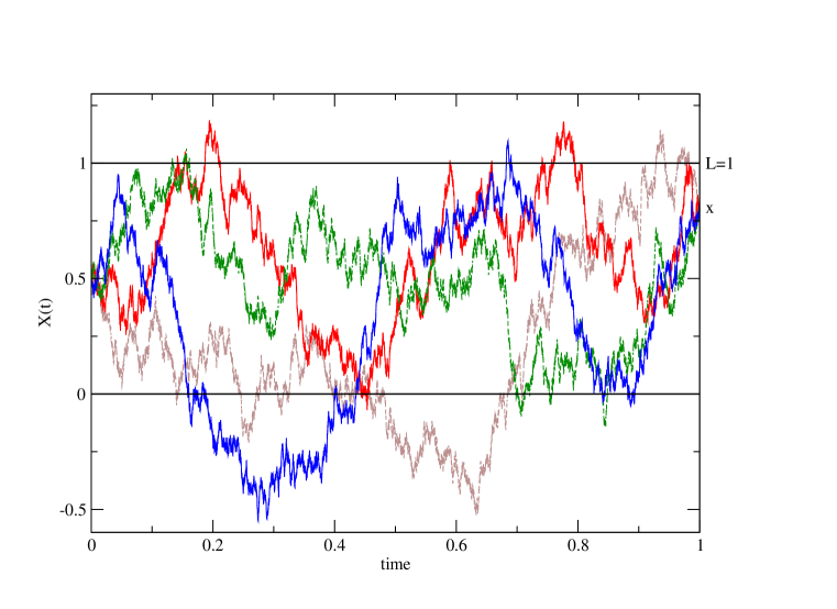
Figure 2: Examples of simulated trajectories $x(t)$ of the Brownian bridge on the interval $t\in[0,1]$ that illustrate the four contributions of ${\hat{\cal C}}_{s}(x,A,B|x_{0})$ in Eq 65. The four trajectories $x(t)$ start from $x_{0}=0.5$ at time $t=0$ and end at $x=0.8$ at time $t=1$ with two non-vanishing local times $A>0$ and $B>0$, but have different last-passage and first-passage properties: the blue trajectory corresponding to $x_{last}=0=x_{first}$ contributes to the first term [00] of Eq 65 given by Eq. 66; the red trajectory corresponding to $x_{last}=L=x_{first}$ contributes to the second term [LL] of Eq 65 given by Eq. 67; the green trajectory corresponding to $x_{last}=0$ and $x_{first}=L$ contributes to the third term [0L] of Eq 65 given by Eq. 68; the brown trajectory corresponding to $x_{last}=L$ and $x_{first}=0$ contributes to the fourth term [L0] of Eq 65 given by Eq. 69. The time step used in the discretization is $dt=10^{-4}$

III Distribution $\Pi_{t}(A,B|x_{0})=\int dxP_{t}(x,A,B|x_{0})$ of the two local times $A$ and $B$ at time $t$

In this section, we focus on the joint distribution $\Pi_{t}(A,B|x_{0})$ of the local times $A$ and $B$ at time $t$ if one starts at position $x_{0}$.

III.1 Decomposition of the distribution $\Pi_{t}(A,B|x_{0})=\int dxP_{t}(x,A,B|x_{0})$ into four contributions

The integration over the final position $x$ of the joint propagator $P_{t}(x,A,B|x_{0})$ of Eq. 18

$$\Pi_{t}(A,B|x_{0}) \equiv\int_{-\infty}^{+\infty}dxP_{t}(x,A,B|x_{0})$$ (70)

$$=\delta(A)\delta(B)S^{abs(0,L)}_{t}(x_{0})+\theta(A>0)\delta(B){\cal A}^{]-\infty,L[}_{t}(A|x_{0})+\delta(A)\theta(B>0){\cal B}^{]0,+\infty[}_{t}(B|x_{0})$$

$$+\theta(A>0)\theta(B>0){\cal C}_{t}(A,B|x_{0})$$

involves the four contributions :

(1) the first contribution corresponding to the integration over $x$ of $G^{abs(0,L)}_{t}(x|x_{0})$ of Eq. 19 represents the survival probability at time $t$ when starting at $x_{0}$ in the presence of absorbing boundaries at positions $x=0$ and $x=L$

$$S^{abs(0,L)}_{t}(x_{0}) =\int_{-\infty}^{+\infty}dxG^{abs(0,L)}_{t}(x|x_{0})$$ (71)

$$=\theta(x_{0}<0)S^{]-\infty,0[}_{t}(x_{0})+\theta(0<x_{0}<L)S^{]0,L[}_{t}(x_{0})+\theta(x_{0}>L)S^{]L,+\infty[}_{t}(x_{0})$$

so that it can be decomposed into the survival probabilities in the three regions $]-\infty,0[$, $]0,L[$ and $]L,+\infty[$.

(2) the second contribution corresponding to the integration over $x$ of ${\cal A}^{abs(L)}_{t}(x,A|x_{0})$ of Eq. 20 is non-vanishing only for $x_{0}<L$

$${\cal A}^{]-\infty,L[}_{t}(A|x_{0})\equiv\int_{-\infty}^{+\infty}dx{\cal A}^{abs(L)}_{t}(x,A|x_{0})=\theta(x_{0}<L){\cal A}^{]-\infty,L[}_{t}(A|x_{0})$$ (72)

(3) the third contribution corresponding to the integration over $x$ of ${\cal B}^{abs(0)}_{t}(x,B|x_{0})$ of Eq. 21 is non-vanishing only for $x_{0}>0$

$${\cal B}^{]0,+\infty[}_{t}(B|x_{0})\equiv\int_{-\infty}^{+\infty}dx{\cal B}^{abs(0)}_{t}(x,B|x_{0})=\theta(x_{0}>0){\cal B}^{]0,+\infty[}_{t}(B|x_{0})$$ (73)

(4) the fourth contribution reads

$${\cal C}_{t}(A,B|x_{0})\equiv\int_{-\infty}^{+\infty}dx{\cal C}_{t}(x,A,B|x_{0})$$ (74)

III.2 Time-Laplace transform ${\hat{\Pi}}_{s}(A,B|x_{0})$ with its four contributions

The time-Laplace transform of Eq. 70

$${\hat{\Pi}}_{s}(A,B|x_{0}) \equiv\int_{0}^{+\infty}dte^{-st}\Pi_{t}(A,B|x_{0})$$ (75)

$$=\delta(A)\delta(B){\hat{S}}^{abs(0,L)}_{s}(x_{0})+\theta(A>0)\delta(B){\hat{\cal A}}^{]-\infty,L[}_{s}(A|x_{0})+\delta(A)\theta(B>0){\hat{\cal B}}^{]0,+\infty[}_{s}(B|x_{0})$$

$$+\theta(A>0)\theta(B>0){\hat{\cal C}}_{s}(A,B|x_{0})$$

can be computed via the integration over $x$ of ${\hat{P}}_{s}(x,A,B|x_{0})$ of Eq. 33

$${\hat{\Pi}}_{s}(A,B|x_{0})=\int_{-\infty}^{+\infty}dx{\hat{P}}_{s}(x,A,B|x_{0})$$ (76)

so that one needs to integrate over $x$ the various contributions computed in the previous section. The normalization of the propagator $G_{t}(x|x_{0})$

$$\int_{-\infty}^{+\infty}dxG_{t}(x|x_{0})=1$$ (77)

translates for its Laplace transform into

$$\int_{-\infty}^{+\infty}dx{\hat{G}}_{s}(x|x_{0})=\int_{0}^{+\infty}dte^{-st}\int_{-\infty}^{+\infty}dxG_{t}(x|x_{0})=\int_{0}^{+\infty}dte^{-st}=\frac{1}{s}$$ (78)

III.3 First contribution ${\hat{S}}^{abs(0,L)}_{s}(x_{0})$

Using Eq. 78, the integration over $x$ of Eq. 35 corresponding to the Laplace transform ${\hat{S}}^{abs(0,L)}_{s}(x_{0})$ of the survival probability $S^{abs(0,L)}_{t}(x_{0})$ of Eq. 71 reads

$${\hat{S}}^{abs(0,L)}_{s}(x_{0}) \equiv\int_{-\infty}^{+\infty}dx{\hat{G}}^{abs(0,L)}_{s}(x|x_{0})$$ (79)

$$=\frac{1}{s}\left[1-\frac{{\hat{G}}_{s}(L|L){\hat{G}}_{s}(0|x_{0})-{\hat{G}}_{s}(0|L){\hat{G}}_{s}(L|x_{0})+{\hat{G}}_{s}(0|0){\hat{G}}_{s}(L|x_{0})-{\hat{G}}_{s}(L|0){\hat{G}}_{s}(0|x_{0})}{\Delta_{s}}\right]$$

$$=\frac{1}{s}\left[1-\frac{{\hat{G}}^{abs(L)}_{s}(0|x_{0})}{{\hat{G}}^{abs(L)}_{s}(0|0)}-\frac{{\hat{G}}^{abs(0)}_{s}(L|x_{0})}{{\hat{G}}^{abs(0)}_{s}(L|L)}\right]$$

with its simplifications of Eq. 71 in the two extreme regions $]-\infty,0[$ and $]L,+\infty[$

$${\hat{S}}^{]-\infty,0[}_{s}(x_{0}) =\frac{1}{s}\left[1-\frac{{\hat{G}}^{abs(L)}_{s}(0|x_{0})}{{\hat{G}}^{abs(L)}_{s}(0|0)}\right]$$

$${\hat{S}}^{]L,+\infty[}_{s}(x_{0}) =\frac{1}{s}\left[1-\frac{{\hat{G}}^{abs(0)}_{s}(L|x_{0})}{{\hat{G}}^{abs(0)}_{s}(L|L)}\right]$$ (80)

III.4 Second contribution ${\hat{\cal A}}^{]-\infty,L[}_{s}(A|x_{0})$

Using Eq. 78, the integration over $x$ of $\alpha_{s}^{[00]}(x|x_{0})$ of Eq. 40

$$\alpha_{s}^{]-\infty,L[}(x_{0}) \equiv\int_{-\infty}^{+\infty}dx\alpha_{s}^{[00]}(x|x_{0})=\int_{-\infty}^{+\infty}dx\left[{\hat{G}}_{s}(x|0)-\frac{{\hat{G}}_{s}(x|L){\hat{G}}_{s}(L|0)}{{\hat{G}}_{s}(L|L)}\right]\frac{{\hat{G}}^{abs(L)}_{s}(0|x_{0})}{\left[{\hat{G}}^{abs(L)}_{s}(0|0)\right]^{2}}$$ (81)

$$=\frac{1}{s}\left[1-\frac{{\hat{G}}_{s}(L|0)}{{\hat{G}}_{s}(L|L)}\right]\frac{{\hat{G}}^{abs(L)}_{s}(0|x_{0})}{\left[{\hat{G}}^{abs(L)}_{s}(0|0)\right]^{2}}$$

that is non-vanishing only for $x_{0}\in]-\infty,0[$ allows to obtain the integration over $x$ of the contribution ${\cal A}^{abs(L)}_{s}(x,A|x_{0})$ of Eq. 42

$${\hat{\cal A}}^{]-\infty,L[}_{s}(A|x_{0})\equiv\int_{-\infty}^{+\infty}dx{\cal A}^{abs(L)}_{s}(x,A|x_{0})=\alpha_{s}^{]-\infty,L[}(x_{0})e^{-\frac{A}{{\hat{G}}^{abs(L)}_{s}(0|0)}}$$ (82)

III.5 Third contribution ${\hat{\cal B}}^{]0,+\infty[}_{s}(B|x_{0})$

Using Eq. 78, the integration over $x$ of $\beta_{s}^{[LL]}(x|x_{0})$ of Eq. 47

$$\beta_{s}^{]0,+\infty[}(x_{0}) \equiv\int_{-\infty}^{+\infty}dx\beta_{s}^{[LL]}(x|x_{0})=\int_{-\infty}^{+\infty}dx\left[{\hat{G}}_{s}(x|L)-\frac{{\hat{G}}_{s}(x|0){\hat{G}}_{s}(0|L)}{{\hat{G}}_{s}(0|0)}\right]\frac{{\hat{G}}^{abs(0)}_{s}(L|x_{0})}{\left[{\hat{G}}^{abs(0)}_{s}(L|L)\right]^{2}}$$ (83)

$$=\frac{1}{s}\left[1-\frac{{\hat{G}}_{s}(0|L)}{{\hat{G}}_{s}(0|0)}\right]\frac{{\hat{G}}^{abs(0)}_{s}(L|x_{0})}{\left[{\hat{G}}^{abs(0)}_{s}(L|L)\right]^{2}}$$

that is non-vanishing only for $x_{0}\in]0,+\infty[$ allows to obtain the integration over $x$ of the contribution ${\cal B}^{abs(0)}_{s}(x,B|x_{0})$ of Eq. 49

$${\hat{\cal B}}^{]0,+\infty[}_{s}(B|x_{0})\equiv\int_{-\infty}^{+\infty}dx{\cal B}^{abs(0)}_{s}(x,B|x_{0})=\beta_{s}^{]0,+\infty[}(x_{0})e^{-\frac{B}{{\hat{G}}^{abs(0)}_{s}(L|L)}}$$ (84)

III.6 Fourth contribution ${\hat{\cal C}}_{s}(A,B|x_{0})$

The integration over $x$ of $\gamma_{s}(x|x_{0})$ of Eq. 57

$$\gamma_{s}(x_{0}) \equiv\int_{-\infty}^{+\infty}dx\gamma_{s}(x|x_{0})=\gamma_{s}^{]-\infty,L[}(x_{0})+\gamma_{s}^{]0,+\infty[}(x_{0})$$ (85)

involves the two following terms using Eq. 78

$$\gamma_{s}^{]-\infty,L[}(x_{0}) \equiv\int_{-\infty}^{+\infty}dx\gamma_{s}^{[L0]}(x|x_{0})=\int_{-\infty}^{+\infty}dx\left(\frac{\left[{\hat{G}}_{s}(x|L)-\frac{{\hat{G}}_{s}(x|0){\hat{G}}_{s}(0|L)}{{\hat{G}}_{s}(0|0)}\right]}{{\hat{G}}^{abs(0)}_{s}(L|L)}\right)\frac{{\hat{G}}_{s}(L|0)}{\Delta_{s}}\left(\frac{{\hat{G}}^{abs(L)}_{s}(0|x_{0})}{{\hat{G}}^{abs(L)}_{s}(0|0)}\right)$$

$$=\left(\frac{\left[1-\frac{{\hat{G}}_{s}(0|L)}{{\hat{G}}_{s}(0|0)}\right]}{{\hat{G}}^{abs(0)}_{s}(L|L)}\right)\frac{{\hat{G}}_{s}(L|0)}{s\Delta_{s}}\left(\frac{{\hat{G}}^{abs(L)}_{s}(0|x_{0})}{{\hat{G}}^{abs(L)}_{s}(0|0)}\right)$$

$$\gamma_{s}^{]0,+\infty[}(x_{0}) \equiv\int_{-\infty}^{+\infty}dx\gamma_{s}^{[0L]}(x|x_{0})=\int_{-\infty}^{+\infty}dx\left(\frac{\left[{\hat{G}}_{s}(x|0)-\frac{{\hat{G}}_{s}(x|L){\hat{G}}_{s}(L|0)}{{\hat{G}}_{s}(L|L)}\right]}{{\hat{G}}^{abs(L)}_{s}(0|0)}\right)\frac{{\hat{G}}_{s}(0|L)}{\Delta_{s}}\left(\frac{{\hat{G}}^{abs(0)}_{s}(L|x_{0})}{{\hat{G}}^{abs(0)}_{s}(L|L)}\right)$$ (86)

$$=\left(\frac{\left[1-\frac{{\hat{G}}_{s}(L|0)}{{\hat{G}}_{s}(L|L)}\right]}{{\hat{G}}^{abs(L)}_{s}(0|0)}\right)\frac{{\hat{G}}_{s}(0|L)}{s\Delta_{s}}\left(\frac{{\hat{G}}^{abs(0)}_{s}(L|x_{0})}{{\hat{G}}^{abs(0)}_{s}(L|L)}\right)$$

The integration over $x$ of the three terms of Eq. 52

$${\hat{\cal C}}^{[\alpha]}_{s}(A,B|x_{0})\equiv\int_{-\infty}^{+\infty}dx{\cal C}^{[\alpha]}_{s}(x,A,B|x_{0})=\alpha_{s}^{]-\infty,L[}(x_{0})c_{s}e^{-\frac{A}{{\hat{G}}^{abs(L)}_{s}(0|0)}}e^{-\frac{B}{{\hat{G}}^{abs(0)}_{s}(L|L)}}\frac{\sqrt{A}}{\sqrt{B}}I_{1}\left(2c_{s}\sqrt{AB}\right)$$

$${\hat{\cal C}}^{[\beta]}_{s}(A,B|x_{0})\equiv\int_{-\infty}^{+\infty}dx{\cal C}^{[\beta]}_{s}(x,A,B|x_{0})=\beta_{s}^{]0,+\infty[}(x_{0})c_{s}e^{-\frac{A}{{\hat{G}}^{abs(L)}_{s}(0|0)}}e^{-\frac{B}{{\hat{G}}^{abs(0)}_{s}(L|L)}}\frac{\sqrt{B}}{\sqrt{A}}I_{1}\left(2c_{s}\sqrt{AB}\right)$$

$${\hat{\cal C}}^{[\gamma]}_{s}(A,B|x_{0})\equiv\int_{-\infty}^{+\infty}dx{\cal C}^{[\gamma]}_{s}(x,A,B|x_{0})=\gamma_{s}(x_{0})e^{-\frac{A}{{\hat{G}}^{abs(L)}_{s}(0|0)}}e^{-\frac{B}{{\hat{G}}^{abs(0)}_{s}(L|L)}}I_{0}\left(2c_{s}\sqrt{AB}\right)$$ (87)

yields that the total contribution ${\hat{\cal C}}_{s}(A,B|x_{0})$ of Eq 51 reads

$${\hat{\cal C}}_{s}(A,B|x_{0})={\hat{\cal C}}^{[\alpha]}_{s}(A,B|x_{0})+{\hat{\cal C}}^{[\beta]}_{s}(A,B|x_{0})+{\hat{\cal C}}^{[\gamma]}_{s}(A,B|x_{0})$$

$$=e^{-\frac{A}{{\hat{G}}^{abs(L)}_{s}(0|0)}}e^{-\frac{B}{{\hat{G}}^{abs(0)}_{s}(L|L)}}\left[\left(\alpha_{s}^{]-\infty,L[}(x_{0})\frac{\sqrt{A}}{\sqrt{B}}+\beta_{s}^{]0,+\infty[}(x_{0})\frac{\sqrt{B}}{\sqrt{A}}\right)c_{s}I_{1}\left(2c_{s}\sqrt{AB}\right)+\gamma_{s}(x_{0})I_{0}\left(2c_{s}\sqrt{AB}\right)\right]$$ (88)

In particular, the asymptotic behaviors of Eq. 55 for the modified Bessel functions $I_{0}(z)$ and $I_{1}(z)$ for large argument $z\to+\infty$ yield the following asymptotic behaviors for large $(AB)$ of the three terms

$${\hat{\cal C}}^{[\alpha]}_{s}(A,B|x_{0}) \mathop{\simeq}_{(AB)\to+\infty}\frac{\alpha_{s}^{]-\infty,L[}(x_{0})\sqrt{c_{s}}A^{\frac{1}{4}}}{2\sqrt{\pi}B^{\frac{3}{4}}}e^{-\frac{A}{{\hat{G}}^{abs(L)}_{s}(0|0)}-\frac{B}{{\hat{G}}^{abs(0)}_{s}(L|L)}+2c_{s}\sqrt{AB}}$$

$${\hat{\cal C}}^{[\beta]}_{s}(A,B|x_{0}) \mathop{\simeq}_{(AB)\to+\infty}\frac{\beta_{s}^{]0,+\infty[}(x_{0})\sqrt{c_{s}}B^{\frac{1}{4}}}{2\sqrt{\pi}A^{\frac{3}{4}}}e^{-\frac{A}{{\hat{G}}^{abs(L)}_{s}(0|0)}-\frac{B}{{\hat{G}}^{abs(0)}_{s}(L|L)}+2c_{s}\sqrt{AB}}$$

$${\hat{\cal C}}^{[\gamma]}_{s}(A,B|x_{0}) \mathop{\simeq}_{(AB)\to+\infty}\frac{\gamma_{s}(x_{0})}{2\sqrt{\pi c_{s}}A^{\frac{1}{4}}B^{\frac{1}{4}}}e^{-\frac{A}{{\hat{G}}^{abs(L)}_{s}(0|0)}-\frac{B}{{\hat{G}}^{abs(0)}_{s}(L|L)}+2c_{s}\sqrt{AB}}$$ (89)

so that the global asymptotic behavior for large $(AB)$ is given by

$${\hat{\cal C}}_{s}(A,B|x_{0})={\hat{\cal C}}^{[\alpha]}_{s}(A,B|x_{0})+{\hat{\cal C}}^{[\beta]}_{s}(A,B|x_{0})+{\hat{\cal C}}^{[\gamma]}_{s}(A,B|x_{0})$$

$$\mathop{\simeq}_{(AB)\to+\infty}\frac{1}{2\sqrt{\pi}}\left[\sqrt{c_{s}}\left(\frac{\alpha_{s}^{]-\infty,L[}(x_{0})A^{\frac{1}{4}}}{B^{\frac{3}{4}}}+\frac{\beta_{s}^{]0,+\infty[}(x_{0})B^{\frac{1}{4}}}{A^{\frac{3}{4}}}\right)+\frac{\gamma_{s}(x_{0})}{\sqrt{c_{s}}A^{\frac{1}{4}}B^{\frac{1}{4}}}\right]e^{-\frac{A}{{\hat{G}}^{abs(L)}_{s}(0|0)}-\frac{B}{{\hat{G}}^{abs(0)}_{s}(L|L)}+2c_{s}\sqrt{AB}}$$ (90)

IV Joint distribution $\Pi_{t}(A,B|x_{0})$ of the local times $A(t)$ and $B(t)$ for large time $t$

In this section, we analyze the joint distribution $\Pi_{t}(A,B|x_{0})$ of the two local times $A(t)$ and $B(t)$ in the limit of large time $t\to+\infty$.

IV.1 When $X(t)$ is transient : the two local times $(A,B)$ remain finite random variables for $t\to+\infty$

When the diffusion process $X(t)$ is transient, then the Laplace transform ${\hat{G}}_{s}(x|x_{0})$ of the propagator $G_{t}(x|x_{0})$ remains finite for $s=0$

$${\hat{G}}_{s=0}(x|x_{0})<+\infty$$ (91)

Then the two local times $A$ and $B$ will remain finite random variables for $t\to+\infty$ with the following notation for their limit distribution obtained from Eq. 70

$$\Pi_{\infty}(A,B|x_{0}) =\lim_{t\to+\infty}\Pi_{t}(A,B|x_{0})$$ (92)

$$=\delta(A)\delta(B)S^{abs(0,L)}_{\infty}(x_{0})+\theta(A>0)\delta(B){\cal A}^{]-\infty,L[}_{\infty}(A|x_{0})+\delta(A)\theta(B>0){\cal B}^{]0,+\infty[}_{\infty}(B|x_{0})$$

$$+\theta(A>0)\theta(B>0){\cal C}_{\infty}(A,B|x_{0})$$

These contributions involving the infinite-time limit $t\to+\infty$ can be obtained from their Laplace transforms by considering the limit $s\to 0$ as follows : the first contribution can be computed from Eq. 79

$$S^{abs(0,L)}_{\infty}(x_{0})=\lim_{s\to 0}\left[s{\hat{S}}^{abs(0,L)}_{s}(x_{0})\right]=1-\frac{{\hat{G}}^{abs(L)}_{0}(0|x_{0})}{{\hat{G}}^{abs(L)}_{0}(0|0)}-\frac{{\hat{G}}^{abs(0)}_{0}(L|x_{0})}{{\hat{G}}^{abs(0)}_{0}(L|L)}$$ (93)

while the second contribution can be computed from Eq. 82

$${\cal A}^{]-\infty,L[}_{\infty}(A|x_{0})=\lim_{s\to 0}\left[s{\hat{\cal A}}^{]-\infty,L[}_{s}(A|x_{0})\right]=\left[1-\frac{{\hat{G}}_{0}(L|0)}{{\hat{G}}_{0}(L|L)}\right]\frac{{\hat{G}}^{abs(L)}_{0}(0|x_{0})}{\left[{\hat{G}}^{abs(L)}_{0}(0|0)\right]^{2}}e^{-\frac{A}{{\hat{G}}^{abs(L)}_{0}(0|0)}}$$ (94)

and the third contribution from Eq. 84

$${\cal B}^{]0,+\infty[}_{\infty}(B|x_{0})=\lim_{s\to 0}\left[s{\hat{\cal B}}^{]0,+\infty[}_{s}(B|x_{0})\right]=\left[1-\frac{{\hat{G}}_{0}(0|L)}{{\hat{G}}_{0}(0|0)}\right]\frac{{\hat{G}}^{abs(0)}_{0}(L|x_{0})}{\left[{\hat{G}}^{abs(0)}_{0}(L|L)\right]^{2}}e^{-\frac{B}{{\hat{G}}^{abs(0)}_{0}(L|L)}}$$ (95)

Finally the three terms of Eq. 87 allow to compute

$${\cal C}^{[\alpha]}_{\infty}(A,B|x_{0})=\lim_{s\to 0}\left[s{\hat{\cal C}}^{[\alpha]}_{s}(A,B|x_{0})\right]=\left[1-\frac{{\hat{G}}_{0}(L|0)}{{\hat{G}}_{0}(L|L)}\right]\frac{{\hat{G}}^{abs(L)}_{0}(0|x_{0})}{\left[{\hat{G}}^{abs(L)}_{0}(0|0)\right]^{2}}c_{0}e^{-\frac{A}{G^{abs(L)}_{0}(0|0)}}e^{-\frac{B}{G^{abs(0)}_{0}(L|L)}}\frac{\sqrt{A}}{\sqrt{B}}I_{1}\left(2c_{0}\sqrt{AB}\right)$$

$${\cal C}^{[\beta]}_{\infty}(A,B|x_{0})=\lim_{s\to 0}\left[s{\hat{\cal C}}^{[\beta]}_{s}(A,B|x_{0})\right]=\left[1-\frac{{\hat{G}}_{0}(0|L)}{{\hat{G}}_{0}(0|0)}\right]\frac{{\hat{G}}^{abs(0)}_{0}(L|x_{0})}{\left[{\hat{G}}^{abs(0)}_{0}(L|L)\right]^{2}}c_{0}e^{-\frac{A}{G^{abs(L)}_{0}(0|0)}}e^{-\frac{B}{G^{abs(0)}_{0}(L|L)}}\frac{\sqrt{B}}{\sqrt{A}}I_{1}\left(2c_{0}\sqrt{AB}\right)$$

$${\cal C}^{[\gamma]}_{\infty}(A,B|x_{0})=\lim_{s\to 0}\left[s{\hat{\cal C}}^{[\gamma]}_{s}(A,B|x_{0})\right]=e^{-\frac{A}{G^{abs(L)}_{0}(0|0)}}e^{-\frac{B}{G^{abs(0)}_{0}(L|L)}}I_{0}\left(2c_{0}\sqrt{AB}\right)$$

$$\times\left[\left(\frac{\left[1-\frac{{\hat{G}}_{0}(0|L)}{{\hat{G}}_{0}(0|0)}\right]}{{\hat{G}}^{abs(0)}_{0}(L|L)}\right)\frac{{\hat{G}}_{0}(L|0)}{\Delta_{0}}\left(\frac{{\hat{G}}^{abs(L)}_{0}(0|x_{0})}{{\hat{G}}^{abs(L)}_{0}(0|0)}\right)+\left(\frac{\left[1-\frac{{\hat{G}}_{0}(L|0)}{{\hat{G}}_{0}(L|L)}\right]}{{\hat{G}}^{abs(L)}_{0}(0|0)}\right)\frac{{\hat{G}}_{0}(0|L)}{\Delta_{0}}\left(\frac{{\hat{G}}^{abs(0)}_{0}(L|x_{0})}{{\hat{G}}^{abs(0)}_{0}(L|L)}\right)\right]$$ (96)

so that the fourth contribution of Eq. 92 reads

$${\cal C}_{\infty}(A,B|x_{0}) ={\cal C}^{[\alpha]}_{\infty}(A,B|x_{0})+{\cal C}^{[\beta]}_{\infty}(A,B|x_{0})+{\cal C}^{[\gamma]}_{\infty}(A,B|x_{0})$$

$$=e^{-\frac{A}{G^{abs(L)}_{0}(0|0)}}e^{-\frac{B}{G^{abs(0)}_{0}(L|L)}}\left(\frac{{\hat{G}}^{abs(L)}_{0}(0|x_{0})}{{\hat{G}}^{abs(L)}_{0}(0|0)}\right)$$

$$\times \left[\frac{c_{0}\left(1-\frac{{\hat{G}}_{0}(L|0)}{{\hat{G}}_{0}(L|L)}\right)}{{\hat{G}}^{abs(L)}_{0}(0|0)}\frac{\sqrt{A}}{\sqrt{B}}I_{1}\left(2c_{0}\sqrt{AB}\right)+\frac{{\hat{G}}_{0}(L|0)\left(1-\frac{{\hat{G}}_{0}(0|L)}{{\hat{G}}_{0}(0|0)}\right)}{\Delta_{0}{\hat{G}}^{abs(0)}_{0}(L|L)}I_{0}\left(2c_{0}\sqrt{AB}\right)\right]$$

$$+e^{-\frac{A}{G^{abs(L)}_{0}(0|0)}}e^{-\frac{B}{G^{abs(0)}_{0}(L|L)}}\left(\frac{{\hat{G}}^{abs(0)}_{0}(L|x_{0})}{{\hat{G}}^{abs(0)}_{0}(L|L)}\right)$$

$$\times \left[\frac{c_{0}\left(1-\frac{{\hat{G}}_{0}(0|L)}{{\hat{G}}_{0}(0|0)}\right)}{{\hat{G}}^{abs(0)}_{0}(L|L)}\frac{\sqrt{B}}{\sqrt{A}}I_{1}\left(2c_{0}\sqrt{AB}\right)+\frac{{\hat{G}}_{0}(0|L)\left(1-\frac{{\hat{G}}_{0}(L|0)}{{\hat{G}}_{0}(L|L)}\right)}{\Delta_{0}{\hat{G}}^{abs(L)}_{0}(0|0)}I_{0}\left(2c_{0}\sqrt{AB}\right)\right]$$ (97)

IV.2 When $X(t)$ is recurrent : large deviations properties of the two intensive local times $(a,b)$ at large time

When the diffusion process $X(t)$ is recurrent, it is more appropriate to introduce the two intensive local times of Eq. 11 and to analyze their large deviations properties thereby generalizing the previous works concerning the single intensive local time $a$ [2, 16].

IV.2.1 Rate function $I(a,b)$ for the two intensive local times $(a,b)$

Let us plug $A=ta$ and $B=tb$ into Eq. 70 with its four contributions

$$\Pi_{t}(A=ta,B=tb|x_{0}) =\delta(a)\delta(b)\frac{1}{t^{2}}S^{abs(0,L)}_{t}(x_{0})+\theta(a>0)\delta(b)\frac{1}{t}{\cal A}^{]-\infty,L[}_{t}(ta|x_{0})+\delta(a)\theta(b>0)\frac{1}{t}{\cal B}^{]0,+\infty[}_{t}(tb|x_{0})$$ (98)

$$+\theta(a>0)\theta(b>0){\cal C}_{t}(ta,tb|x_{0})$$

Since the leading behavior is the exponential decay with respect to the time $t$ of Eq. 12 that involves the positive rate function $I(a,b)\geq 0$ defined for $a\in[0,+\infty[$ and $b\in[0,+\infty[$, the four contributions of Eq. 98 are then governed by the four different exponential factors

$$S^{abs(0,L)}_{t}(x_{0}) \mathop{\propto}_{t\to+\infty}e^{-tI(a=0,b=0)}$$

$${\cal A}^{]-\infty,L[}_{t}(A=ta|x_{0}) \mathop{\propto}_{t\to+\infty}e^{-tI(a,b=0)}$$

$${\cal B}^{]0,+\infty[}_{t}(B=tb|x_{0}) \mathop{\propto}_{t\to+\infty}e^{-tI(a=0,b)}$$

$${\cal C}_{t}(A=ta,B=tb|x_{0}) \mathop{\propto}_{t\to+\infty}e^{-tI(a,b)}$$ (99)

In the following subsections, the goal is to evaluate at leading order the various contributions including the prefactors in order to have the dependence with respect to the initial position $x_{0}$ that will be needed later to construct conditioned processes. It is more convenient to begin with the fourth contribution ${\cal C}_{t}(A=ta,B=tb|x_{0})$ since it is the only one that involves the full joint rate function $I(a,b)$ of the two variables $a$ and $b$.

IV.2.2 Evaluation of the fourth contribution ${\cal C}_{t}(A=ta,B=tb|x_{0})$ at leading order for large time $t$

The contribution ${\hat{\cal C}}_{s}(A=ta,B=tb|x_{0})$ of Eq. 88 displays the asymptotic behavior given by Eq. 90 for large time $t$

$${\hat{\cal C}}_{s}(A=ta,B=tb|x_{0}) \mathop{\simeq}_{t\to+\infty}\frac{1}{2\sqrt{\pi t}}\left[\frac{\alpha_{s}^{]-\infty,L[}(x_{0})\sqrt{c_{s}}a^{\frac{1}{4}}}{b^{\frac{3}{4}}}+\frac{\beta_{s}^{]0,+\infty[}(x_{0})\sqrt{c_{s}}b^{\frac{1}{4}}}{a^{\frac{3}{4}}}+\frac{\gamma_{s}(x_{0})}{\sqrt{c_{s}}a^{\frac{1}{4}}b^{\frac{1}{4}}}\right]$$ (100)

$$\times e^{-t\left[\frac{a}{{\hat{G}}^{abs(L)}_{s}(0|0)}+\frac{b}{{\hat{G}}^{abs(0)}_{s}(L|L)}-2c_{s}\sqrt{ab}\right]}$$

The Laplace inversion of this asymptotic behavior allows to compute the fourth contribution ${\cal C}_{t}(A=ta,B=tb|x_{0})$ at leading order for large $t$

$${\cal C}_{t}(A=ta,B=tb|x_{0})=\int_{c-i\infty}^{c+i\infty}\frac{ds}{2i\pi}e^{st}{\hat{\cal C}}_{s}(A=ta,B=tb|x_{0})$$ (101)

$$\mathop{\simeq}_{t\to+\infty}\int_{c-i\infty}^{c+i\infty}\frac{ds}{2i\pi}\frac{1}{2\sqrt{\pi t}}\left[\sqrt{c_{s}}\left(\frac{\alpha_{s}^{]-\infty,L[}(x_{0})a^{\frac{1}{4}}}{b^{\frac{3}{4}}}+\frac{\beta_{s}^{]0,+\infty[}(x_{0})b^{\frac{1}{4}}}{a^{\frac{3}{4}}}\right)+\frac{\gamma_{s}(x_{0})}{\sqrt{c_{s}}a^{\frac{1}{4}}b^{\frac{1}{4}}}\right]e^{-t\left[\frac{a}{{\hat{G}}^{abs(L)}_{s}(0|0)}+\frac{b}{{\hat{G}}^{abs(0)}_{s}(L|L)}-2c_{s}\sqrt{ab}-s\right]}$$

For large $t$, the saddle-point evaluation of this integral over $s$ involves the solution $s_{a,b}$ of

$$0=\partial_{s}\left[\frac{a}{{\hat{G}}^{abs(L)}_{s}(0|0)}+\frac{b}{{\hat{G}}^{abs(0)}_{s}(L|L)}-2c_{s}\sqrt{ab}-s\right]$$ (102)

One then needs to make the change of variable

$$s=s_{a,b}+i\omega$$ (103)

and to use the Taylor expansion at second order in $\omega$

$$\left[\frac{a}{{\hat{G}}^{abs(L)}_{s}(0|0)}+\frac{b}{{\hat{G}}^{abs(0)}_{s}(L|L)}-2c_{s}\sqrt{ab}-s\right]_{s=s_{a,b}+i\omega}=I(a,b)+0+\frac{\omega^{2}}{2}K(a,b)+o\left(\omega^{2}\right)$$ (104)

that involves the two functions

$$I(a,b) =\left[\frac{a}{{\hat{G}}^{abs(L)}_{s}(0|0)}+\frac{b}{{\hat{G}}^{abs(0)}_{s}(L|L)}-2c_{s}\sqrt{ab}-s\right]_{s=s_{a,b}}$$

$$K(a,b) =-\left[\partial^{2}_{s}\left(\frac{a}{{\hat{G}}^{abs(L)}_{s}(0|0)}+\frac{b}{{\hat{G}}^{abs(0)}_{s}(L|L)}-2c_{s}\sqrt{ab}-s\right)\right]_{s=s_{a,b}}$$ (105)

The final result for the leading order of Eq. 101 based on the remaining Gaussian integral over $\omega$ reads

$${\cal C}_{t}(A=ta,B=tb|x_{0}) \mathop{\simeq}_{t\to+\infty}\frac{e^{-tI(a,b)}}{2\sqrt{\pi t}}\left[\sqrt{c_{s}}\left(\frac{\alpha_{s}^{]-\infty,L[}(x_{0})a^{\frac{1}{4}}}{b^{\frac{3}{4}}}+\frac{\beta_{s}^{]0,+\infty[}(x_{0})b^{\frac{1}{4}}}{a^{\frac{3}{4}}}\right)+\frac{\gamma_{s}(x_{0})}{\sqrt{c_{s}}a^{\frac{1}{4}}b^{\frac{1}{4}}}\right]_{s=s_{a,b}}\int_{-\infty}^{+\infty}\frac{d\omega}{2\pi}e^{-t\frac{K(a,b)}{2}\omega^{2}}$$ (106)

$$\mathop{\simeq}_{t\to+\infty}\frac{e^{-tI(a,b)}}{2\pi t\sqrt{2K(a,b)}}\left[\sqrt{c_{s}}\left(\frac{\alpha_{s}^{]-\infty,L[}(x_{0})a^{\frac{1}{4}}}{b^{\frac{3}{4}}}+\frac{\beta_{s}^{]0,+\infty[}(x_{0})b^{\frac{1}{4}}}{a^{\frac{3}{4}}}\right)+\frac{\gamma_{s}(x_{0})}{\sqrt{c_{s}}a^{\frac{1}{4}}b^{\frac{1}{4}}}\right]_{s=s_{a,b}}$$

IV.2.3 Evaluation of the second contribution ${\cal A}^{]-\infty,L[}_{t}(A=ta|x_{0})$ at leading order for large time $t$

The second contribution ${\cal A}^{]-\infty,L[}_{t}(A=ta|x_{0})$ can be obtained from the Laplace inverse of ${\hat{\cal A}}^{]-\infty,L[}_{s}(A=ta|x_{0})$ of Eq. 82

$${\cal A}^{]-\infty,L[}_{t}(A=ta|x_{0})=\int_{c-i\infty}^{c+i\infty}\frac{ds}{2i\pi}e^{st}{\hat{\cal A}}^{]-\infty,L[}_{s}(A=ta|x_{0})=\int_{c-i\infty}^{c+i\infty}\frac{ds}{2i\pi}\alpha_{s}^{]-\infty,L[}(x_{0})e^{-t\left[\frac{a}{{\hat{G}}^{abs(L)}_{s}(0|0)}-s\right]}$$ (107)

For large $t$, the saddle-point evaluation of this integral involves the solution $s_{a,0}$ of

$$0=\partial_{s}\left[\frac{a}{{\hat{G}}^{abs(L)}_{s}(0|0)}-s\right]$$ (108)

that corresponds to the special case $b=0$ in Eq. 102. So the Taylor expansion of Eq. 104 for special case $b=0$

$$\left[\frac{a}{{\hat{G}}^{abs(L)}_{s}(0|0)}-s\right]_{s=s_{a,0}+i\omega}=I(a,0)+0+\frac{\omega^{2}}{2}K(a,0)+o\left(\omega^{2}\right)$$ (109)

yields that Eq. 107 reads the leading order

$${\cal A}^{]-\infty,L[}_{t}(A=ta|x_{0}) \mathop{\simeq}_{t\to+\infty}e^{-tI(a,0)}\alpha_{s_{a,0}}^{]-\infty,L[}(x_{0})\int_{-\infty}^{+\infty}\frac{d\omega}{2\pi}e^{-t\frac{K(a,0)}{2}\omega^{2}}$$ (110)

$$\mathop{\simeq}_{t\to+\infty}e^{-tI(a,0)}\frac{\alpha_{s_{a,0}}^{]-\infty,L[}(x_{0})}{\sqrt{2\pi K(a,0)t}}$$

IV.2.4 Evaluation of the third contribution ${\cal B}^{]0,+\infty[}_{t}(B=tb|x_{0})$ at leading order for large time $t$

The third contribution ${\cal B}^{]0,+\infty[}_{t}(B=tb|x_{0})$ can be obtained from the Laplace inverse of ${\hat{\cal B}}^{]0,+\infty[}_{s}(B=tb|x_{0})$ of Eq. 84

$${\cal B}^{]0,+\infty[}_{t}(B=tb|x_{0})=\int_{c-i\infty}^{c+i\infty}\frac{ds}{2i\pi}e^{st}{\hat{\cal B}}^{]0,+\infty[}_{s}(B=tb|x_{0})=\int_{c-i\infty}^{c+i\infty}\frac{ds}{2i\pi}\beta_{s}^{]0,+\infty[}(x_{0})e^{-t\left[\frac{b}{{\hat{G}}^{abs(0)}_{s}(L|L)}-s\right]}$$ (111)

For large $t$, the saddle-point evaluation of this integral involves the solution $s_{0,b}$ of

$$0=\partial_{s}\left[\frac{b}{{\hat{G}}^{abs(0)}_{s}(L|L)}-s\right]$$ (112)

that corresponds to the special case $a=0$ in Eq. 102. So the Taylor expansion of Eq. 104 for special case $a=0$

$$\left[\frac{b}{{\hat{G}}^{abs(0)}_{s}(L|L)}-s\right]_{s=s_{0,b}+i\omega}=I(0,b)+0+\frac{\omega^{2}}{2}K(0,b)+o\left(\omega^{2}\right)$$ (113)

yields that Eq. 111 reads the leading order

$${\cal B}^{abs(0)}_{t}(B=tb|x_{0}) \mathop{\simeq}_{t\to+\infty}e^{-tI(0,b)}\beta_{s_{0,b}}^{]0,+\infty[}(x_{0})\int_{-\infty}^{+\infty}\frac{d\omega}{2\pi}e^{-t\frac{K(0,b)}{2}\omega^{2}}$$ (114)

$$\mathop{\simeq}_{t\to+\infty}e^{-tI(0,b)}\frac{\beta_{s_{0,b}}^{]0,+\infty[}(x_{0})}{\sqrt{2\pi K(0,b)t}}$$

IV.2.5 Conclusion

Putting everything together, one obtains the asymptotic behavior at leading order for large time $t$ of Eq. 98

$$\Pi_{t}(A=ta,B=tb|x_{0}) \mathop{\simeq}_{t\to+\infty}\delta(a)\delta(b)\frac{1}{t^{2}}S^{abs(0,L)}_{t}(x_{0})$$ (115)

$$+\theta(a>0)\delta(b)\frac{\alpha_{s_{a,0}}^{]-\infty,L[}(x_{0})e^{-tI(a,0)}}{\sqrt{2\pi K(a,0)}t^{\frac{3}{2}}}$$

$$+\delta(a)\theta(b>0)\frac{\beta_{s_{0,b}}^{]0,+\infty[}(x_{0})e^{-tI(0,b)}}{\sqrt{2\pi K(0,b)}t^{\frac{3}{2}}}$$

$$+\theta(a>0)\theta(b>0)\frac{e^{-tI(a,b)}}{2\pi t\sqrt{2K(a,b)}}\left[\sqrt{c_{s}}\left(\frac{\alpha_{s}^{]-\infty,L[}(x_{0})a^{\frac{1}{4}}}{b^{\frac{3}{4}}}+\frac{\beta_{s}^{]0,+\infty[}(x_{0})b^{\frac{1}{4}}}{a^{\frac{3}{4}}}\right)+\frac{\gamma_{s}(x_{0})}{\sqrt{c_{s}}a^{\frac{1}{4}}b^{\frac{1}{4}}}\right]_{s=s_{a,b}}$$

V Statistics of the sum $\Sigma(t)=A(t)+B(t)$ of the two local times $A(t)$ and $B(t)$

In this section, we focus on the sum $\Sigma(t)$ of the two local times

$$\Sigma(t)\equiv A(t)+B(t) =\int_{0}^{t}d\tau\left[\delta(X(\tau))+\delta(X(\tau)-L)\right]$$ (116)

whose statistical properties are simpler.

V.1 Propagator $P_{t}(x,\Sigma|x_{0})$ for the position $x$ and the sum $\Sigma$ of the two local times

V.1.1 Singular contribution in $\delta(\Sigma)$ and regular contribution in $\theta(\Sigma>0)$

The joint propagator $P_{t}(x,\Sigma|x_{0})$ can be computed from the joint propagator $P_{t}(x,A,B|x_{0})$ of Eq. 18 with its four contributions

$$P_{t}(x,\Sigma|x_{0}) =\int_{0}^{+\infty}dA\int_{0}^{+\infty}dBP_{t}(x,A,B|x_{0})\delta(\Sigma-(A+B))$$ (117)

$$=\delta(\Sigma)G^{abs(0,L)}_{t}(x|x_{0})+\theta(\Sigma>0)\Upsilon_{t}(x,\Sigma|x_{0})$$

where the regular contribution $\Upsilon_{t}(x,\Sigma|x_{0})$ reads

$$\Upsilon_{t}(x,\Sigma|x_{0})={\cal A}^{abs(L)}_{t}(x,\Sigma|x_{0})+{\cal B}^{abs(0)}_{t}(x,\Sigma|x_{0})+\int_{0}^{\Sigma}dA{\cal C}_{t}(x,A,\Sigma-A|x_{0})$$ (118)

or equivalently for the time Laplace transform

$${\hat{P}}_{s}(x,\Sigma|x_{0})\equiv\int_{0}^{+\infty}dte^{-st}P_{t}(x,\Sigma|x_{0})=\delta(\Sigma){\hat{G}}^{abs(0,L)}_{s}(x|x_{0})+\theta(\Sigma>0){\hat{\Upsilon}}_{s}(x,\Sigma|x_{0})$$ (119)

with

$${\hat{\Upsilon}}_{s}(x,\Sigma|x_{0})={\hat{\cal A}}_{s}(x,\Sigma|x_{0})+{\hat{\cal B}}_{s}(x,\Sigma|x_{0})+\int_{0}^{\Sigma}dA{\hat{\cal C}}_{s}(x,A,\Sigma-A|x_{0})$$ (120)

However, instead of computing the convolution of the last term, it is simpler to consider the further Laplace transform with respect to $\Sigma$ of parameter $p$ as we now describe.

V.1.2 Explicit regular contribution ${\hat{\tilde{\Upsilon}}}_{s,p}(x|x_{0})$

The further Laplace transform of Eq. 119 with respect to $\Sigma$ of parameter $p$ corresponds to ${\hat{\tilde{P}}}_{s,p,p}(x|x_{0})$ computed in Eq. 31 for the special case $q=p$

$$\int_{0}^{+\infty}d\Sigma e^{-p\Sigma}{\hat{P}}_{s}(x,\Sigma|x_{0})={\hat{G}}^{abs(0,L)}_{s}(x|x_{0})+{\hat{\tilde{\Upsilon}}}_{s,p}(x|x_{0})=\int_{0}^{+\infty}dAe^{-pA}\int_{0}^{+\infty}dBe^{-pB}{\hat{P}}_{s}(x,A,B|x_{0})$$

$$={\hat{\tilde{P}}}_{s,p,p}(x|x_{0})={\hat{G}}_{s}(x|x_{0})-\frac{p^{2}\Delta_{s}\Omega_{s}(x|x_{0})+p\left[{\hat{G}}_{s}(x|0){\hat{G}}_{s}(0|x_{0})+{\hat{G}}_{s}(x|L){\hat{G}}_{s}(L|x_{0})\right]}{\Delta_{s}p^{2}+p{\hat{G}}_{s}(0|0)+p{\hat{G}}_{s}(L|L)+1}$$ (121)

Using Eq. 35, one obtains the explicit form of ${\hat{\tilde{\Upsilon}}}_{s,p}(x|x_{0})$

$${\hat{\tilde{\Upsilon}}}_{s,p}(x|x_{0}) =\Omega_{s}(x|x_{0})-\frac{p^{2}\Delta_{s}\Omega_{s}(x|x_{0})+p\left[{\hat{G}}_{s}(x|0){\hat{G}}_{s}(0|x_{0})+{\hat{G}}_{s}(x|L){\hat{G}}_{s}(L|x_{0})\right]}{\Delta_{s}p^{2}+p\left[{\hat{G}}_{s}(0|0)+{\hat{G}}_{s}(L|L)\right]+1}$$ (122)

$$=\frac{\Omega_{s}(x|x_{0})+p\Delta_{s}\left[\alpha_{s}^{[00]}(x|x_{0})+\beta_{s}^{[LL]}(x|x_{0})\right]}{\Delta_{s}p^{2}+p\left[{\hat{G}}_{s}(0|0)+{\hat{G}}_{s}(L|L)\right]+1}$$

in terms of the functions $\alpha_{s}^{[00]}(x|x_{0})$ and $\beta_{s}^{[LL]}(x|x_{0})$ introduced in Eqs 40 and 47.

V.1.3 Laplace inversion of ${\hat{\tilde{\Upsilon}}}_{s,p}(x|x_{0})$ with respect to $p$ to obtain ${\hat{\Upsilon}}_{s}(x,\Sigma|x_{0})$

The factorization of the denominator of Eq. 122

$$\Delta_{s}p^{2}+p\left[{\hat{G}}_{s}(0|0)+{\hat{G}}_{s}(L|L)\right]+1=\Delta_{s}(p+\lambda_{s}^{+})(p+\lambda_{s}^{-})$$ (123)

involves the two positive functions $\lambda_{s}^{\pm}>0$ given by

$$\lambda_{s}^{\pm} \equiv\frac{\left[{\hat{G}}_{s}(0|0)+{\hat{G}}_{s}(L|L)\right]\pm\sqrt{\left[{\hat{G}}_{s}(0|0)+{\hat{G}}_{s}(L|L)\right]^{2}-4\Delta_{s}}}{2\Delta_{s}}$$ (124)

$$=\frac{\left[{\hat{G}}_{s}(0|0)+{\hat{G}}_{s}(L|L)\right]\pm\sqrt{\left[{\hat{G}}_{s}(0|0)-{\hat{G}}_{s}(L|L)\right]^{2}+4{\hat{G}}_{s}(0|L){\hat{G}}_{s}(L|0)}}{2\Delta_{s}}$$

$$=\frac{1}{2}\left[\frac{1}{{\hat{G}}^{abs(0)}_{s}(L|L)}+\frac{1}{{\hat{G}}^{abs(L)}_{s}(0|0)}\pm D_{s}\right]$$

where we have introduced the following notation for the difference

$$D_{s}\equiv\lambda_{s}^{+}-\lambda_{s}^{-}=\sqrt{\left(\frac{1}{{\hat{G}}^{abs(0)}_{s}(L|L)}-\frac{1}{{\hat{G}}^{abs(L)}_{s}(0|0)}\right)^{2}+4c_{s}^{2}}$$ (125)

So the partial fraction decomposition of Eq. 122 with respect to the variable $p$ reduces to

$${\hat{\tilde{\Upsilon}}}_{s,p}(x|x_{0})=\frac{\Lambda_{s}^{+}(x|x_{0})}{p+\lambda_{s}^{+}}+\frac{\Lambda_{s}^{-}(x|x_{0})}{p+\lambda_{s}^{-}}$$ (126)

where the identification with Eq. 122 yields that the two numerators $\Lambda_{s}^{\pm}(x|x_{0})$ satisfy the following system using Eq. 375

$$\lambda_{s}^{-}\Lambda_{s}^{+}(x|x_{0})+\lambda_{s}^{+}\Lambda_{s}^{-}(x|x_{0}) =\frac{\Omega_{s}(x|x_{0})}{\Delta_{s}}=\frac{\alpha_{s}^{[00]}(x|x_{0})}{{\hat{G}}^{abs(0)}_{s}(L|L)}+\frac{\beta_{s}^{[LL]}(x|x_{0})}{{\hat{G}}^{abs(L)}_{s}(0|0)}+\gamma_{s}(x|x_{0})$$

$$\Lambda_{s}^{+}(x|x_{0})+\Lambda_{s}^{-}(x|x_{0}) =\alpha_{s}^{[00]}(x|x_{0})+\beta_{s}^{[LL]}(x|x_{0})$$ (127)

and thus read

$$\Lambda_{s}^{+}(x|x_{0}) =\frac{\alpha_{s}^{[00]}(x|x_{0})\left[\lambda_{s}^{+}-\frac{1}{{\hat{G}}^{abs(0)}_{s}(L|L)}\right]+\beta_{s}^{[LL]}(x|x_{0})\left[\lambda_{s}^{+}-\frac{1}{{\hat{G}}^{abs(L)}_{s}(0|0)}\right]-\gamma_{s}(x|x_{0})}{D_{s}}$$

$$\Lambda_{s}^{-}(x|x_{0}) =\frac{\alpha_{s}^{[00]}(x|x_{0})\left[\frac{1}{{\hat{G}}^{abs(0)}_{s}(L|L)}-\lambda_{s}^{-}\right]+\beta_{s}^{[LL]}(x|x_{0})\left[\frac{1}{{\hat{G}}^{abs(L)}_{s}(0|0)}-\lambda_{s}^{-}\right]+\gamma_{s}(x|x_{0})}{D_{s}}$$ (128)

The Laplace inversion with respect to $p$ of Eq. 126 yields the following two exponential functions with respect to $\Sigma$ of parameters $\lambda_{s}^{\pm}$

$${\hat{\Upsilon}}_{s}(x,\Sigma|x_{0})=\Lambda_{s}^{+}(x|x_{0})e^{-\lambda_{s}^{+}\Sigma}+\Lambda_{s}^{-}(x|x_{0})e^{-\lambda_{s}^{-}\Sigma}$$ (129)

V.2 Distribution $\Pi_{t}(\Sigma|x_{0})=\int dxP_{t}(x,\Sigma|x_{0})$ of the sum $\Sigma$ at time $t$

The distribution $\Pi_{t}(\Sigma|x_{0})$ of the sum $\Sigma$ at time $t$ when starting at position $x_{0}$ can be obtained from the integration over the final position $x$ of the $P_{t}(x,\Sigma|x_{0})$ of Eq. 117

$$\Pi_{t}(\Sigma|x_{0})\equiv\int_{-\infty}^{+\infty}dxP_{t}(x,\Sigma|x_{0})=\delta(\Sigma)S^{abs(0,L)}_{t}(x_{0})+\theta(\Sigma>0)\Upsilon_{t}(\Sigma|x_{0})$$ (130)

where

$$\Upsilon_{t}(\Sigma|x_{0})\equiv\int_{-\infty}^{+\infty}dx\Upsilon_{t}(x,\Sigma|x_{0})$$ (131)

Its time Laplace transform ${\hat{\Upsilon}}_{s}(\Sigma|x_{0})$ can be obtained from the integration over $x$ of ${\hat{\Upsilon}}_{s}(x,\Sigma|x_{0})$ Eq. 129

$${\hat{\Upsilon}}_{s}(\Sigma|x_{0})=\int_{-\infty}^{+\infty}dx{\hat{\Upsilon}}_{s}(x,\Sigma|x_{0})=\Lambda_{s}^{+}(x_{0})e^{-\lambda_{s}^{+}\Sigma}+\Lambda_{s}^{-}(x_{0})e^{-\lambda_{s}^{-}\Sigma}$$ (132)

where the amplitudes $\Lambda_{s}^{\pm}(x_{0})$ can be computed using the explicit expressions of the functions $\alpha_{s}^{]-\infty,L[}(x_{0})$, $\beta_{s}^{]0,+\infty[}(x_{0})$ and $\gamma_{s}(x_{0})$ of Eqs 81, 83 and 85

$$\Lambda_{s}^{+}(x_{0}) =\int_{-\infty}^{+\infty}dx\Lambda_{s}^{+}(x|x_{0})=\frac{\alpha_{s}^{]-\infty,L[}(x_{0})\left[\lambda_{s}^{+}-\frac{1}{{\hat{G}}^{abs(0)}_{s}(L|L)}\right]+\beta_{s}^{]0,+\infty[}(x_{0})\left[\lambda_{s}^{+}-\frac{1}{{\hat{G}}^{abs(L)}_{s}(0|0)}\right]-\gamma_{s}(x_{0})}{D_{s}}$$

$$=\lambda_{s}^{+}\frac{\left({\hat{G}}_{s}(L|L)-{\hat{G}}_{s}(L|0)-\frac{1}{\lambda_{s}^{+}}\right)\frac{{\hat{G}}^{abs(L)}_{s}(0|x_{0})}{{\hat{G}}^{abs(L)}_{s}(0|0)}+\left({\hat{G}}_{s}(0|0)-{\hat{G}}_{s}(0|L)-\frac{1}{\lambda_{s}^{+}}\right)\frac{{\hat{G}}^{abs(0)}_{s}(L|x_{0})}{{\hat{G}}^{abs(0)}_{s}(L|L)}}{s\left[\frac{1}{\lambda_{s}^{-}}-\frac{1}{\lambda_{s}^{+}}\right]}$$

$$\Lambda_{s}^{-}(x_{0}) =\int_{-\infty}^{+\infty}dx\Lambda_{s}^{-}(x|x_{0})=\frac{\alpha_{s}^{]-\infty,L[}(x_{0})\left[\frac{1}{{\hat{G}}^{abs(0)}_{s}(L|L)}-\lambda_{s}^{-}\right]+\beta_{s}^{[LL]}(x_{0})\left[\frac{1}{{\hat{G}}^{abs(L)}_{s}(0|0)}-\lambda_{s}^{-}\right]+\gamma_{s}(x_{0})}{D_{s}}$$ (133)

$$=\lambda_{s}^{-}\frac{\left(\frac{1}{\lambda_{s}^{-}}-\left[{\hat{G}}_{s}(L|L)-{\hat{G}}_{s}(L|0)\right]\right)\frac{{\hat{G}}^{abs(L)}_{s}(0|x_{0})}{{\hat{G}}^{abs(L)}_{s}(0|0)}+\left(\frac{1}{\lambda_{s}^{-}}-\left[{\hat{G}}_{s}(0|0)-{\hat{G}}_{s}(0|L)\right]\right)\frac{{\hat{G}}^{abs(0)}_{s}(L|x_{0})}{{\hat{G}}^{abs(0)}_{s}(L|L)}}{s\left[\frac{1}{\lambda_{s}^{-}}-\frac{1}{\lambda_{s}^{+}}\right]}$$

so that the normalization of Eq. 132 over $\Sigma$

$$\int_{0}^{+\infty}d\Sigma{\hat{\Upsilon}}_{s}(\Sigma|x_{0})=\frac{\Lambda_{s}^{+}(x_{0})}{\lambda_{s}^{+}}+\frac{\Lambda_{s}^{-}(x_{0})}{\lambda_{s}^{-}}=\frac{1}{s}\left[\frac{{\hat{G}}^{abs(L)}_{s}(0|x_{0})}{{\hat{G}}^{abs(L)}_{s}(0|0)}+\frac{{\hat{G}}^{abs(0)}_{s}(L|x_{0})}{{\hat{G}}^{abs(0)}_{s}(L|L)}\right]=\frac{1}{s}-{\hat{S}}^{abs(0,L)}_{s}(x_{0})$$ (134)

is complementary to ${\hat{S}}^{abs(0,L)}_{s}(x_{0})$ of Eq. 79 as it should.

V.3 Moments $m^{[k]}_{t}(x_{0})=\langle\Sigma^{k}(t)\rangle_{x_{0}}$ of the sum $\Sigma(t)$ when starting at $x_{0}$

The moments of order $k>0$ of $\Sigma$ at time $t$ can be computed from the distribution $\Pi_{t}(\Sigma|x_{0})$ of Eq. 130

$$m^{[k]}_{t}(x_{0})=\langle\Sigma^{k}(t)\rangle_{x_{0}}=\int_{0}^{+\infty}d\Sigma\Sigma^{k}\Pi_{t}(\Sigma|x_{0})=\int_{0}^{+\infty}d\Sigma\Sigma^{k}\Upsilon_{t}(\Sigma|x_{0})$$ (135)

Their time-Laplace transforms can be computed from the time Laplace transform ${\hat{\Upsilon}}_{s}(\Sigma|x_{0})$ of Eq. 131

$${\hat{m}}^{[k]}_{s}(x_{0}) \equiv\int_{0}^{+\infty}dte^{-st}m^{[k]}_{t}(x_{0})=\int_{0}^{+\infty}d\Sigma\Sigma^{k}{\hat{\Upsilon}}_{s}(\Sigma|x_{0})=\int_{0}^{+\infty}d\Sigma\Sigma^{k}\left[\Lambda_{s}^{+}(x_{0})e^{-\lambda_{s}^{+}\Sigma}+\Lambda_{s}^{-}(x_{0})e^{-\lambda_{s}^{-}\Sigma}\right]$$ (136)

$$=k!\left(\frac{\Lambda_{s}^{+}(x_{0})}{(\lambda_{s}^{+})^{k+1}}+\frac{\Lambda_{s}^{-}(x_{0})}{(\lambda_{s}^{-})^{k+1}}\right)$$

V.4 When $X(t)$ is transient : the sum $\Sigma(t)$ remain a finite random variable for $t\to+\infty$

As already explained in subsection IV.1, the two local times $(A,B)$ remain finite random variables for $t\to+\infty$. It is thus interesting to write the asymptotic distribution of the sum $\Sigma$ obtained from Eq. 130

$$\Pi_{\infty}(\Sigma|x_{0})=\lim_{t\to+\infty}\Pi_{t}(\Sigma|x_{0})=\delta(\Sigma)S^{abs(0,L)}_{\infty}(x_{0})+\theta(\Sigma>0)\Upsilon_{\infty}(\Sigma|x_{0})$$ (137)

where the singular contribution $S^{abs(0,L)}_{\infty}(x_{0})$ has been already given in Eq. 93, while the regular contribution $\Upsilon_{\infty}(\Sigma|x_{0})$ involving the infinite-time limit $t\to+\infty$ can be obtained from the Laplace transform ${\hat{\Upsilon}}_{s}(\Sigma|x_{0})$ of Eq. 132 by considering the limit $s\to 0$ of

$$\Upsilon_{\infty}(\Sigma|x_{0}) =\lim_{s\to 0}\left[s{\hat{\Upsilon}}_{s}(\Sigma|x_{0})\right]=\lim_{s\to 0}\left[s\Lambda_{s}^{+}(x_{0})e^{-\lambda_{s}^{+}\Sigma}+s\Lambda_{s}^{-}(x_{0})e^{-\lambda_{s}^{-}\Sigma}\right]$$ (138)

$$=\xi^{+}(x_{0})e^{-\lambda_{0}^{+}\Sigma}+\xi^{-}(x_{0})e^{-\lambda_{0}^{-}\Sigma}$$

where the two amplitudes $\xi^{\pm}(x_{0})$ can be obtained from Eq. 133

$$\xi^{+}(x_{0}) =\lim_{s\to 0}\left[s\Lambda_{s}^{+}(x_{0})\right]$$

$$=\lambda_{0}^{+}\frac{\left({\hat{G}}_{0}(L|L)-{\hat{G}}_{0}(L|0)-\frac{1}{\lambda_{0}^{+}}\right)\frac{{\hat{G}}^{abs(L)}_{0}(0|x_{0})}{{\hat{G}}^{abs(L)}_{0}(0|0)}+\left({\hat{G}}_{0}(0|0)-{\hat{G}}_{0}(0|L)-\frac{1}{\lambda_{0}^{+}}\right)\frac{{\hat{G}}^{abs(0)}_{0}(L|x_{0})}{{\hat{G}}^{abs(0)}_{0}(L|L)}}{\left[\frac{1}{\lambda_{0}^{-}}-\frac{1}{\lambda_{0}^{+}}\right]}$$

$$\xi^{-}(x_{0}) =\lim_{s\to 0}\left[s\Lambda_{s}^{-}(x_{0})\right]$$ (139)

$$=\lambda_{0}^{-}\frac{\left(\frac{1}{\lambda_{0}^{-}}-\left[{\hat{G}}_{0}(L|L)-{\hat{G}}_{0}(L|0)\right]\right)\frac{{\hat{G}}^{abs(L)}_{0}(0|x_{0})}{{\hat{G}}^{abs(L)}_{0}(0|0)}+\left(\frac{1}{\lambda_{0}^{-}}-\left[{\hat{G}}_{0}(0|0)-{\hat{G}}_{0}(0|L)\right]\right)\frac{{\hat{G}}^{abs(0)}_{0}(L|x_{0})}{{\hat{G}}^{abs(0)}_{0}(L|L)}}{\left[\frac{1}{\lambda_{0}^{-}}-\frac{1}{\lambda_{0}^{+}}\right]}$$

so that the normalization of Eq. 138 over $\Sigma$

$$\int_{0}^{+\infty}d\Sigma\Upsilon_{\infty}(\Sigma|x_{0})=\frac{\xi^{+}(x_{0})}{\lambda_{0}^{+}}+\frac{\xi^{-}(x_{0})}{\lambda_{0}^{-}}=\frac{{\hat{G}}^{abs(L)}_{0}(0|x_{0})}{{\hat{G}}^{abs(L)}_{0}(0|0)}+\frac{{\hat{G}}^{abs(0)}_{0}(L|x_{0})}{{\hat{G}}^{abs(0)}_{0}(L|L)}=1-S^{abs(0,L)}_{\infty}(x_{0})$$ (140)

is complementary to $S^{abs(0,L)}_{\infty}(x_{0})$ of Eq. 93 as it should.

V.5 When $X(t)$ is recurrent : large deviations properties of the intensive sum $\sigma=\frac{\Sigma(t)}{t}$ at large time $t$

When $X(t)$ is recurrent, it is interesting to analyze the large deviations properties of the intensive sum of the two local times $A(t)$ and $B(t)$

$$\sigma=\frac{\Sigma(t)}{t}=\frac{A(t)+B(t)}{t}$$ (141)

V.5.1 Evaluation of the distribution $\Pi_{t}(\Sigma=\sigma t|x_{0})$ at leading order in $t$

The distribution $\Pi_{t}(\Sigma=\sigma t|x_{0})$ of $\Sigma=\sigma t$ for $\sigma\in]0,+\infty[$ can be evaluated from the Laplace inversion of Eq. 132

$$\Upsilon_{t}(\Sigma=\sigma t|x_{0}) =\int_{c-i\infty}^{c+i\infty}\frac{ds}{2i\pi}e^{st}{\hat{\Upsilon}}_{s}(\Sigma|x_{0})=\int_{c-i\infty}^{c+i\infty}\frac{ds}{2i\pi}\left[\Lambda_{s}^{+}(x_{0})e^{-t\left[\sigma\lambda_{s}^{+}-s\right]}+\Lambda_{s}^{-}(x_{0})e^{-t\left[\sigma\lambda_{s}^{-}-s\right]}\right]$$ (142)

For large $t$, the dominant exponential is the second term involving $\lambda_{s}^{-}$ (since $\lambda_{s}^{-}<\lambda_{s}^{+}$ in Eq. 124), so that the saddle-point evaluation involves the solution $s_{\sigma}$ of

$$0=\partial_{s}\left[\sigma\lambda_{s}^{-}-s\right]=\sigma\partial_{s}\lambda_{s}^{-}-1$$ (143)

The change of variable

$$s=s_{\sigma}+i\omega$$ (144)

and the Taylor expansion at second order in $\omega$

$$\left[\sigma\lambda_{s}^{-}-s\right]_{s=s_{\sigma}+i\omega}=J(\sigma)+0+\frac{\omega^{2}}{2}\chi(\sigma)+o\left(\omega^{2}\right)$$ (145)

that involves the two functions

$$J(\sigma) =\left[\sigma\lambda_{s}^{-}-s\right]_{s=s_{\sigma}}$$

$$\chi(\sigma) =-\sigma\left[\partial^{2}_{s}\lambda_{s}^{-}\right]_{s=s_{\sigma}}$$ (146)

leads to the final result for the leading order of Eq. 142

$$\Pi_{t}(\Sigma=\sigma t|x_{0}) \mathop{\simeq}_{t\to+\infty}\Lambda_{s_{\sigma}}^{-}(x_{0})e^{-tJ(\sigma)}\int_{-\infty}^{+\infty}\frac{d\omega}{2\pi}e^{-t\frac{\chi(\sigma)}{2}\omega^{2}}=\frac{\Lambda_{s_{\sigma}}^{-}(x_{0})e^{-tJ(\sigma)}}{\sqrt{2\pi t\chi(\sigma)}}$$ (147)

V.5.2 Link between the rate function $J(\sigma)$ of the intensive sum $\sigma=a+b$ and the joint rate function $I(a,b)$

The integration over $x$ of Eq. 118

$$\Upsilon_{t}(\Sigma|x_{0})={\cal A}^{abs(L)}_{t}(\Sigma|x_{0})+{\cal B}^{abs(0)}_{t}(\Sigma|x_{0})+\int_{0}^{\Sigma}dA{\cal C}_{t}(A,\Sigma-A|x_{0})$$ (148)

reads for $\Sigma=\sigma t$

$$\Upsilon_{t}(\Sigma=\sigma t|x_{0})={\cal A}^{abs(L)}_{t}(t\sigma|x_{0})+{\cal B}^{abs(0)}_{t}(t\sigma|x_{0})+\int_{0}^{\sigma}tda{\cal C}_{t}(ta,t(\sigma-a)|x_{0})$$ (149)

where the two first terms are governed by the rate functions $I(a=\sigma,b=0)$ and $I(a=0,b=\sigma)$ of Eq. 99, while the convolution of the last term involves the rate function $I(a,b=\sigma-a)$

$$\int_{0}^{\sigma}da{\cal C}_{t}(ta,t(\sigma-a)|x_{0})\mathop{\propto}_{t\to+\infty}\int_{0}^{\sigma}dae^{-tI(a,\sigma-a)}\mathop{\propto}_{t\to+\infty}e^{-tJ(\sigma)}$$ (150)

As a consequence, the rate function $J(\sigma)$ should correspond to the optimization of the joint rate function $I(a,\sigma-a)$ over all possible values $a\in[0,\sigma]$

$$J(\sigma)=\min_{0\leq a\leq\sigma}I(a,\sigma-a)$$ (151)

Since the rate function $I(a,b)$ is the minimum over $s$ of the function in the exponential in Eq. 101

$$I(a,b)=\min_{s}\left[\frac{a}{{\hat{G}}^{abs(L)}_{s}(0|0)}+\frac{b}{{\hat{G}}^{abs(0)}_{s}(L|L)}-2c_{s}\sqrt{ab}-s\right]$$ (152)

one can exchange the two minimizations to rewrite Eq. 151 as

$$J(\sigma)=\min_{s}\min_{0\leq a\leq\sigma}\left[\frac{a}{{\hat{G}}^{abs(L)}_{s}(0|0)}+\frac{\sigma-a}{{\hat{G}}^{abs(0)}_{s}(L|L)}-2c_{s}\sqrt{a(\sigma-a)}-s\right]$$ (153)

The minimization over $a$

$$0 =\partial_{a}\left[\frac{a}{{\hat{G}}^{abs(L)}_{s}(0|0)}+\frac{\sigma-a}{{\hat{G}}^{abs(0)}_{s}(L|L)}-2c_{s}\sqrt{a(\sigma-a)}-s\right]$$ (154)

$$=\frac{1}{{\hat{G}}^{abs(L)}_{s}(0|0)}-\frac{1}{{\hat{G}}^{abs(0)}_{s}(L|L)}-c_{s}\frac{\sigma-2a}{\sqrt{a(\sigma-a)}}$$

yields the explicit optimal value

$$a_{opt} =\frac{\sigma}{2}\left(1+\frac{\frac{1}{{\hat{G}}^{abs(0)}_{s}(L|L)}-\frac{1}{{\hat{G}}^{abs(L)}_{s}(0|0)}}{\sqrt{\left[\frac{1}{{\hat{G}}^{abs(0)}_{s}(L|L)}-\frac{1}{{\hat{G}}^{abs(L)}_{s}(0|0)}\right]^{2}+4c_{s}^{2}}}\right)$$ (155)

$$=\frac{\sigma}{2}\left(1+\frac{\frac{1}{{\hat{G}}^{abs(0)}_{s}(L|L)}-\frac{1}{{\hat{G}}^{abs(L)}_{s}(0|0)}}{D_{s}}\right)$$

that can be plugged into Eq. 153 to obtain

$$J(\sigma) =\min_{s}\left[\frac{a_{opt}}{{\hat{G}}^{abs(L)}_{s}(0|0)}+\frac{\sigma-a_{opt}}{{\hat{G}}^{abs(0)}_{s}(L|L)}-2c_{s}\sqrt{a_{opt}(\sigma-a_{opt})}-s\right]$$

$$= \min_{s}\left[\frac{\sigma}{2}\left(\frac{1}{{\hat{G}}^{abs(0)}_{s}(L|L)}+\frac{1}{{\hat{G}}^{abs(L)}_{s}(0|0)}-D_{s}\right)-s\right]$$

$$= \min_{s}\left[\sigma\lambda_{s}^{-}-s\right]$$ (156)

so that one recovers the function $\lambda_{s}^{-}$ of Eq. 124, as it should for consistency with the direct calculation of Eqs 143 and 146 of the previous subsection.

VI Conditioned processes involving the two local times

In this section, the goal is to construct conditioned joint processes $[X^{*}(t),A^{*}(t),B^{*}(t)]$ satisfying certain constraints involving the two local times, thereby generalizing our previous work [16] concerning the conditioning with respect to the single local time $A(t)$.

VI.1 Conditioned Bridge towards the local times $[A^{*}_{T},B^{*}_{T}]$ at the time horizon $T$

If the conditioning is towards the local times $[A^{*}_{T},B^{*}_{T}]$ at the time horizon $T$, without any condition on the final position $x_{T}$, the conditioned distribution of the position $x$ and the local times $(A,B)$ at some interior time $t\in]0,T[$ involves the unconditioned joint distribution $\Pi_{t_{2}-t_{1}}(A_{2}-A_{1},B_{2}-B_{1}|x_{1})$ of the two increments $[A_{2}-A_{1},B_{2}-B_{1}]$ during the time interval $(t_{2}-t_{1})$ described in section III

$$P^{[A_{T}^{*},B_{T}^{*}]}_{T}(x,A,B,t)=\frac{\Pi_{T-t}(A_{T}^{*}-A,B_{T}^{*}-B|x)P_{t}(x,A,B|x_{0})}{\Pi_{T}(A_{T}^{*},B_{T}^{*}|x_{0})}$$ (157)

The corresponding conditioned process $[X^{*}(t),A^{*}(t),B^{*}(t)]$ then satisfies the SDE of Eq. 13 where the conditioned drift $\mu^{[A_{T}^{*},B_{T}^{*}]}_{T}(x,A,B,t)$ is given by Eq. 14. The decomposition of $\Pi_{T-t}(A_{T}^{*}-A,B_{T}^{*}-B|x)$ into its four contributions of Eq. 70

$$\Pi_{T-t}(A_{T}^{*}-A,B_{T}^{*}-B|x)=\delta(A_{T}^{*}-A)\delta(B_{T}^{*}-B)S^{abs(0,L)}_{T-t}(x)+\theta(A_{T}^{*}>A)\delta(B_{T}^{*}-B){\cal A}^{]-\infty,L[}_{T-t}(A_{T}^{*}-A|x)$$

$$+\delta(A_{T}^{*}-A)\theta(B_{T}^{*}>B){\cal B}^{]0,+\infty[}_{T-t}(B_{T}^{*}-B|x)+\theta(A_{T}^{*}>A)\theta(B_{T}^{*}>B){\cal C}_{T-t}(A_{T}^{*}-A,B_{T}^{*}-B|x)$$ (158)

yields that the conditioned dynamics can be decomposed into the following regimes :

(1) for $[0\leq A<A_{T}^{*},0\leq B<B_{T}^{*}]$ where the two local times $A$ and $B$ have not yet reached their conditioned final values $A_{T}^{*}$ and $B_{T}^{*}$, the conditioned drift of Eq. 14 involves the contribution ${\cal C}_{T-t}(A_{T}^{*}-A,B_{T}^{*}-B|x)$

$$\mu^{[A_{T}^{*},B_{T}^{*}]}_{T}(x,A<A_{T}^{*},B<B_{T}^{*},t)=\mu(x)+\partial_{x}\ln{\cal C}_{T-t}(A_{T}^{*}-A,B_{T}^{*}-B|x)$$ (159)

(2) the regime (1) ends when either $A$ or $B$ reaches its conditioned final value, so the next regime (2) contains two possibilities :

(2-A) if $B$ has already reached its conditioned final value $B=B_{T}^{*}$ while $A$ has not yet reached its conditioned final value $A_{T}^{*}$, then the conditioned drift of Eq. 14 involves the contribution ${\cal A}^{]-\infty,L[}_{T-t}(A_{T}^{*}-A|x)$

$$\mu^{[A_{T}^{*},B_{T}^{*}]}_{T}(x,A<A_{T}^{*},B=B_{T}^{*},t)=\mu(x)+\partial_{x}\ln{\cal A}^{]-\infty,L[}_{T-t}(A_{T}^{*}-A|x)$$ (160)

(2-B) if $A$ has already reached its conditioned final value $A=A_{T}^{*}$ while $B$ has not yet reached its conditioned final value $B_{T}^{*}$, then the conditioned drift of Eq. 14 involves the contribution ${\cal B}^{]0,+\infty[}_{T-t}(B_{T}^{*}-B|x)$

$$\mu^{[A_{T}^{*},B_{T}^{*}]}_{T}(x,A=A_{T}^{*},B<B_{T}^{*},t)=\mu(x)+\partial_{x}\ln{\cal B}^{]0,+\infty[}_{T-t}(B_{T}^{*}-B|x)$$ (161)

(3) in the last regime $[A=A_{T}^{*},B=B_{T}^{*}]$ where the two local times $A$ and $B$ have already reached their conditioned final values $A_{T}^{*}$ and $B_{T}^{*}$, the conditioned drift of Eq. 14 involves the contribution $S^{abs(0,L)}_{T-t}(x)$, since the process cannot visit $0$ or $L$ anymore

$$\mu^{[A_{T}^{*},B_{T}^{*}]}_{T}(x,A=A_{T}^{*},B=B_{T}^{*},t)=\mu(x)+\partial_{x}\ln S^{abs(0,L)}_{T-t}(x)$$ (162)

It is now interesting to consider two possibilities in the limit of the infinite horizon $T\to+\infty$, as described in the two next subsections.

VI.2 Conditioning towards the finite local times $[A_{\infty},B_{\infty}]$ for the infinite horizon $T\to+\infty$

If one wishes to impose the finite asymptotic local times $A_{\infty}<+\infty$ and $B_{\infty}<+\infty$ at the infinite horizon $T\to+\infty$, one needs to analyze the limit of the infinite horizon $T\to+\infty$ for the conditioned drift of Eq 14

$$\mu^{[A_{\infty}^{*},B_{\infty}^{*}]}_{\infty}(x,A,B)=\mu(x)+\lim_{\tau\to+\infty}\partial_{x}\ln\Pi_{\tau}(A_{\infty}^{*}-A,B_{\infty}^{*}-B|x)$$ (163)

with its different expressions for the various regimes of Eqs 159 160 161 162

$$\mu^{[A_{\infty}^{*},B_{\infty}^{*}]}_{\infty}(x,A<A_{\infty}^{*},B<B_{\infty}^{*}) =\mu(x)+\lim_{\tau\to+\infty}\partial_{x}\ln{\cal C}_{\tau}(A_{\infty}^{*}-A,B_{\infty}^{*}-B|x)$$

$$\mu^{[A_{\infty}^{*},B_{\infty}^{*}]}_{\infty}(x,A<A_{\infty}^{*},B=B_{\infty}^{*}) =\mu(x)+\lim_{\tau\to+\infty}\partial_{x}\ln{\cal A}^{]-\infty,L[}_{\tau}(A_{\infty}^{*}-A|x)$$

$$\mu^{[A_{\infty}^{*},B_{\infty}^{*}]}_{\infty}(x,A=A_{\infty}^{*},B<B_{\infty}^{*}) =\mu(x)+\lim_{\tau\to+\infty}\partial_{x}\ln{\cal B}^{]0,+\infty[}_{\tau}(B_{\infty}^{*}-B|x)$$

$$\mu^{[A_{\infty}^{*},B_{\infty}^{*}]}_{\infty}(x,A=A_{\infty}^{*},B=B_{\infty}^{*}) =\mu(x)+\lim_{\tau\to+\infty}\partial_{x}\ln S^{abs(0,L)}_{\tau}(x)$$ (164)

VI.3 Conditioning towards the intensive local times $a_{*}=\frac{A_{T}^{*}}{T}$ and $b_{*}=\frac{B_{T}^{*}}{T}$ for large time horizon $T\to+\infty$

If one wishes to impose instead the fixed intensive local times $a_{*}>0$ and $b_{*}>0$ for large time horizon $T\to+\infty$, one needs to plug the values

$$A_{T}^{*} =Ta_{*}$$

$$B_{T}^{*} =Tb_{*}$$ (165)

into the conditioned drift of Eq. 14

$$\mu^{[Ta_{*},Tb_{*}]}_{T}(x,A,B,t)=\mu(x)+\partial_{x}\ln\Pi_{T-t}(Ta_{*}-A,Tb_{*}-B|x)$$ (166)

and to use the large-time behavior of Eq. 115 that involves the corresponding intensive local times $a_{t}$ and $b_{t}$ on the time interval $(T-t)$

$$a_{t} \equiv\frac{Ta_{*}-A}{T-t}\mathop{\simeq}_{T\to+\infty}a_{*}$$

$$b_{t} \equiv\frac{Tb_{*}-B}{T-t}\mathop{\simeq}_{T\to+\infty}b_{*}$$ (167)

that reduces to $a_{*}$ and $b_{*}$ at leading order when $T\to+\infty$. Let us discuss two special cases before the general case $(a_{*}>0,b_{*}>0)$

VI.3.1 Case $a_{*}>0$ and $b_{*}=0$

For $a_{*}>0$ and $b_{*}=0$, the asymptotic behavior of Eq. 115

$$\Pi_{T-t}(Ta_{*}-A,0|x)\mathop{\simeq}_{T\to+\infty}\frac{\alpha_{s_{a_{*},0}}^{]-\infty,L[}(x)e^{-tI(a_{*},0)}}{\sqrt{2\pi K(a_{*},0)}(T-t)^{\frac{3}{2}}}$$ (168)

can be plugged into Eq. 166 to obtain the limit $\mu^{[a_{*},b_{*}=0]}_{\infty}(x)$ of the conditioned drift using Eq. 81

$$\mu^{[a_{*},b_{*}=0]}_{\infty}(x) \equiv\lim_{T\to+\infty}\mu^{[Ta_{*},Tb_{*}]}_{T}(x,A,B,t)=\mu(x)+\partial_{x}\ln\left[\alpha_{s_{a_{*},0}}^{]-\infty,L[}(x)\right]$$ (169)

$$=\mu(x)+\partial_{x}\ln\left[{\hat{G}}^{abs(L)}_{s_{a_{*},0}}(0|x)\right]$$

where $s_{a_{*},0}$ is the solution of Eq. 108

$$0=\partial_{s}\left[\frac{a_{*}}{{\hat{G}}^{abs(L)}_{s}(0|0)}-s\right]=a_{*}\partial_{s}\left[\frac{1}{{\hat{G}}^{abs(L)}_{s}(0|0)}\right]-1$$ (170)

So the conditioned drift of Eq. 169 can be also rewritten in the following parametric form of parameter $s$

$$\mu^{[a_{*}(s),b_{*}=0]}_{\infty}(x) =\mu(x)+\partial_{x}\ln\left[{\hat{G}}^{abs(L)}_{s}(0|x)\right]$$

$$a^{*}(s) =\frac{1}{\partial_{s}\left[\frac{1}{{\hat{G}}^{abs(L)}_{s}(0|0)}\right]}$$ (171)

VI.3.2 Case $a_{*}=0$ and $b_{*}>0$

For $a_{*}=0$ and $b_{*}>0$, the asymptotic behavior of Eq. 115

$$\Pi_{T-t}(0,Tb_{*}-B|x)\mathop{\simeq}_{T\to+\infty}\frac{\beta_{s_{0,b}}^{]0,+\infty[}(x)e^{-tI(0,b)}}{\sqrt{2\pi K(0,b)}t^{\frac{3}{2}}}$$ (172)

can be plugged into Eq. 166 to obtain the limit $\mu^{[a_{*},b_{*}=0]}_{\infty}(x)$ of the conditioned drift using Eq. 83

$$\mu^{[a_{*}=0,b_{*}]}_{\infty}(x) \equiv\lim_{T\to+\infty}\mu^{[Ta_{*},Tb_{*}]}_{T}(x,A,B,t)=\mu(x)+\partial_{x}\ln\left[\beta_{s_{0,b_{*}}}^{]0,+\infty[}(x)\right]$$ (173)

$$=\mu(x)+\partial_{x}\ln\left[{\hat{G}}^{abs(0)}_{s_{0,b_{*}}}(L|x)\right]$$

where $s_{0,b_{*}}$ is the solution of Eq. 112

$$0=\partial_{s}\left[\frac{b_{*}}{{\hat{G}}^{abs(0)}_{s}(L|L)}-s\right]=b_{*}\partial_{s}\left[\frac{1}{{\hat{G}}^{abs(0)}_{s}(L|L)}\right]-1$$ (174)

So the conditioned drift of Eq. 173 can be also written in the following parametric form of parameter $s$

$$\mu^{[a_{*}=0,b_{*}(s)]}_{\infty}(x) =\mu(x)+\partial_{x}\ln\left[{\hat{G}}^{abs(0)}_{s}(L|x)\right]$$

$$b_{*}(s) =\frac{1}{\partial_{s}\left[\frac{1}{{\hat{G}}^{abs(0)}_{s}(L|L)}\right]}$$ (175)

VI.3.3 General case $a_{*}>0$ and $b_{*}>0$

For $a_{*}>0$ and $b_{*}>0$, the asymptotic behavior of Eq. 115

$$\Pi_{T-t}(Ta_{*}-A,Tb_{*}-B|x) \mathop{\simeq}_{T\to+\infty}\frac{e^{-(T-t)I(a_{*},b_{*})}}{2\pi(T-t)\sqrt{2K(a_{*},b_{*})}}\left[\sqrt{c_{s}}\left(\frac{\alpha_{s}^{]-\infty,L[}(x)a_{*}^{\frac{1}{4}}}{b_{*}^{\frac{3}{4}}}+\frac{\beta_{s}^{]0,+\infty[}(x)b_{*}^{\frac{1}{4}}}{a_{*}^{\frac{3}{4}}}\right)+\frac{\gamma_{s}(x)}{\sqrt{c_{s}}a_{*}^{\frac{1}{4}}b_{*}^{\frac{1}{4}}}\right]_{s=s_{a_{*},b_{*}}}$$ (176)

can be plugged into Eq. 166 to obtain the limit $\mu^{[a_{*},b_{*}]}_{\infty}(x)$ of the conditioned drift

$$\mu^{[a_{*},b_{*}]}_{\infty}(x) \equiv\lim_{T\to+\infty}\mu^{[Ta_{*},Tb_{*}]}_{T}(x,A,B,t)=\mu(x)+\partial_{x}\ln\left[\sqrt{c_{s}}\left(\frac{\alpha_{s}^{]-\infty,L[}(x)a_{*}^{\frac{1}{4}}}{b_{*}^{\frac{3}{4}}}+\frac{\beta_{s}^{]0,+\infty[}(x)b_{*}^{\frac{1}{4}}}{a_{*}^{\frac{3}{4}}}\right)+\frac{\gamma_{s}(x)}{\sqrt{c_{s}}a_{*}^{\frac{1}{4}}b_{*}^{\frac{1}{4}}}\right]_{s=s_{a_{*},b_{*}}}$$ (177)

$$=\mu(x)+\partial_{x}\ln\left[c_{s}\left(\sqrt{\frac{a_{*}}{b_{*}}}\alpha_{s}^{]-\infty,L[}(x)+\sqrt{\frac{b_{*}}{a_{*}}}\beta_{s}^{]0,+\infty[}(x)\right)+\gamma_{s}(x)\right]_{s=s_{a_{*},b_{*}}}$$

Using the explicit expressions of Eqs 81 83 85 and 362, this conditioned drift becomes

$$\mu^{[a_{*},b_{*}]}_{\infty}(x)=\mu(x)$$

$$+\partial_{x}\ln\bigg{[}\left(\sqrt{{\hat{G}}_{s}(0|L){\hat{G}}_{s}(L|0)\frac{a_{*}}{b_{*}}}\left[{\hat{G}}_{s}(L|L)-{\hat{G}}_{s}(L|0)\right]+\left[{\hat{G}}_{s}(0|0)-{\hat{G}}_{s}(0|L)\right]{\hat{G}}_{s}(L|0)\right){\hat{G}}_{s}(L|L){\hat{G}}^{abs(L)}_{s}(0|x)$$

$$+\left(\sqrt{{\hat{G}}_{s}(0|L){\hat{G}}_{s}(L|0)\frac{b_{*}}{a_{*}}}\left[{\hat{G}}_{s}(0|0)-{\hat{G}}_{s}(0|L)\right]+\left[{\hat{G}}_{s}(L|L)-{\hat{G}}_{s}(L|0)\right]{\hat{G}}_{s}(0|L)\right){\hat{G}}_{s}(0|0){\hat{G}}^{abs(0)}_{s}(L|x)\bigg{]}_{s=s_{a_{*},b_{*}}}$$ (178)

where $s_{a_{*},b_{*}}$ is the solution of Eq. 102

$$0=\partial_{s}\left[\frac{a_{*}}{{\hat{G}}^{abs(L)}_{s}(0|0)}+\frac{b_{*}}{{\hat{G}}^{abs(0)}_{s}(L|L)}-2c_{s}\sqrt{a_{*}b_{*}}-s\right]$$ (179)

The conditioned drift of Eq. 178 is much simpler in the two external regions :

(i) for $x\in]-\infty,0]$, the function ${\hat{G}}^{abs(0)}_{s}(L|x)$ vanishes, so that Eq. 178 reduces to

$$\mu^{[a_{*},b_{*}]}_{\infty}(x<0)=\mu(x)+\partial_{x}\ln\left[{\hat{G}}^{abs(L)}_{s}(0|x)\right]_{s=s_{a_{*},b_{*}}}$$ (180)

(ii) for $x\in[L,+\infty[$ the function ${\hat{G}}^{abs(L)}_{s}(0|x)$ vanishes, so that Eq. 178 reduces to

$$\mu^{[a_{*},b_{*}]}_{\infty}(x>L)=\mu(x)+\partial_{x}\ln\left[{\hat{G}}^{abs(0)}_{s}(L|x)\right]_{s=s_{a_{*},b_{*}}}$$ (181)

Finally, if one replaces $(a_{*},b_{*})$ by the parametrization

$$a_{*} =\frac{\sigma_{*}(1+r_{*})}{2}$$

$$b_{*} =\frac{\sigma_{*}(1-r_{*})}{2}$$ (182)

involving their sum $\sigma_{*}=a_{*}+b_{*}>0$ and the parameter $r_{*}\in]-1,+1[$ Eq. 179 becomes

$$1=\sigma_{*}\partial_{s}\left[\frac{1+r_{*}}{2{\hat{G}}^{abs(L)}_{s}(0|0)}+\frac{1-r_{*}}{2{\hat{G}}^{abs(0)}_{s}(L|L)}-c_{s}\sqrt{1-r_{*}^{2}}\right]$$ (183)

then the conditioned drift of Eq. 178 can be written in the following parametric form

$$\sigma_{*}(s)=\frac{1}{\partial_{s}\left[\frac{1+r_{*}}{2{\hat{G}}^{abs(L)}_{s}(0|0)}+\frac{1-r_{*}}{2{\hat{G}}^{abs(0)}_{s}(L|L)}-c_{s}\sqrt{1-r_{*}^{2}}\right]}$$

$$\mu^{[\frac{\sigma_{*}(s)(1+r_{*})}{2},\frac{\sigma_{*}(s)(1-r_{*})}{2}]}_{\infty}(x)=\mu(x)$$

$$+\partial_{x}\ln\bigg{[}\left(\sqrt{{\hat{G}}_{s}(0|L){\hat{G}}_{s}(L|0)\frac{1+r_{*}}{1-r_{*}}}\left[{\hat{G}}_{s}(L|L)-{\hat{G}}_{s}(L|0)\right]+\left[{\hat{G}}_{s}(0|0)-{\hat{G}}_{s}(0|L)\right]{\hat{G}}_{s}(L|0)\right){\hat{G}}_{s}(L|L){\hat{G}}^{abs(L)}_{s}(0|x)$$

$$+\left(\sqrt{{\hat{G}}_{s}(0|L){\hat{G}}_{s}(L|0)\frac{1-r_{*}}{1+r_{*}}}\left[{\hat{G}}_{s}(0|0)-{\hat{G}}_{s}(0|L)\right]+\left[{\hat{G}}_{s}(L|L)-{\hat{G}}_{s}(L|0)\right]{\hat{G}}_{s}(0|L)\right){\hat{G}}_{s}(0|0){\hat{G}}^{abs(0)}_{s}(L|x)\bigg{]}$$ (184)

VI.4 Conditioned Bridge towards the sum $\Sigma^{*}_{T}$ at the time horizon $T$

If the conditioning is towards the sum $\Sigma^{*}_{T}$ at time horizon $T$, the conditioned distribution of the position $x$ and the sum $\Sigma$ at some interior time $t\in]0,T[$ involves the unconditioned distribution $\Pi_{t_{2}-t_{1}}(\Sigma_{2}-\Sigma_{1},|x_{1})$ of the increment $(\Sigma_{2}-\Sigma_{1})$ during the time interval $(t_{2}-t_{1})$ described in subsection V.2

$$P^{[\Sigma_{T}^{*}]}_{T}(x,\Sigma,t)=\frac{\Pi_{T-t}(\Sigma_{T}^{*}-\Sigma|x)P_{t}(x,\Sigma|x_{0})}{\Pi_{T}(\Sigma_{T}^{*}|x_{0})}$$ (185)

The corresponding conditioned process $[X^{*}(t),\Sigma^{*}(t)]$ satisfies the following SDE system

$$dX^{*}(t) =\mu^{[\Sigma_{T}^{*}]}_{T}(X^{*}(t),\Sigma^{*}(t),t)dt+dW(t)$$

$$d\Sigma^{*}(t) =\left[\delta(X^{*}(t))+\delta(X^{*}(t)-L)\right]dt$$ (186)

where the conditioned drift $\mu^{[\Sigma_{T}^{*}]}_{T}(x,\Sigma,t)$ reads

$$\mu^{[\Sigma_{T}^{*}]}_{T}(x,\Sigma,t)=\mu(x)+\partial_{x}\ln\Pi_{T-t}(\Sigma_{T}^{*}-\Sigma|x)$$ (187)

The decomposition of $\Pi_{T-t}(\Sigma_{T}^{*}-\Sigma|x)$ into its singular and regular contributions of Eq. 130

$$\Pi_{T-t}(\Sigma_{T}^{*}-\Sigma|x)=\delta(\Sigma_{T}^{*}-\Sigma)S^{abs(0,L)}_{T-t}(x)+\theta(\Sigma_{T}^{*}>\Sigma)\Upsilon_{T-t}(\Sigma_{T}^{*}-\Sigma|x)$$ (188)

yields that the conditioned dynamics can be decomposed into the two regimes :

(i) for $0\leq\Sigma<\Sigma_{T}^{*}$ where the sum $\Sigma$ has not yet reached its conditioned final value $\Sigma_{T}^{*}$, the conditioned drift of Eq. 187 involves the regular contribution $\Upsilon_{T-t}(\Sigma_{T}^{*}-\Sigma|x)$

$$\mu^{[\Sigma_{T}^{*}]}_{T}(x,\Sigma<\Sigma_{T}^{*},t)=\mu(x)+\partial_{x}\ln\Upsilon_{T-t}(\Sigma_{T}^{*}-\Sigma|x)$$ (189)

(ii) for $\Sigma=\Sigma_{T}^{*}$ where the sum $\Sigma$ has already reached its conditioned final value $\Sigma_{T}^{*}$, the conditioned drift of Eq. 187 involves the survival probability $S^{abs(0,L)}_{T-t}(x)$, since the process cannot visit $0$ or $L$ anymore

$$\mu^{[\Sigma_{T}^{*}]}_{T}(x,\Sigma<\Sigma_{T}^{*},t)=\mu(x)+\partial_{x}\ln S^{abs(0,L)}_{T-t}(x)$$ (190)

It is now interesting to consider two possibilities in the limit of the infinite horizon $T\to+\infty$, as described in the two next subsections.

VI.5 Conditioning towards the finite sum $\Sigma_{\infty}^{*}$ for the infinite horizon $T\to+\infty$

If one wishes to impose the finite asymptotic sum $\Sigma_{\infty}^{*}$ at the infinite horizon $T\to+\infty$, one needs to analyze the limit of the infinite horizon $T\to+\infty$ for the conditioned drift of Eq 187

$$\mu^{[\Sigma_{\infty}^{*}]}_{\infty}(x,\Sigma)=\mu(x)+\lim_{\tau\to+\infty}\partial_{x}\ln\Pi_{\tau}(\Sigma_{\infty}^{*}-\Sigma|x)$$ (191)

with its two different expressions for the two regimes of Eqs 189 190

$$\mu^{[\Sigma_{\infty}^{*}]}_{\infty}(x,\Sigma<\Sigma_{\infty}^{*}) =\mu(x)+\lim_{\tau\to+\infty}\partial_{x}\ln\Upsilon_{\tau}(\Sigma_{T}^{*}-\Sigma|x)$$

$$\mu^{[\Sigma_{\infty}^{*}]}_{\infty}(x,\Sigma=\Sigma_{\infty}^{*}) =\mu(x)+\lim_{\tau\to+\infty}\partial_{x}\ln S^{abs(0,L)}_{\tau}(x)$$ (192)

VI.6 Conditioning towards the intensive sum $\sigma_{*}=\frac{\Sigma_{T}^{*}}{T}$ for large time horizon $T\to+\infty$

If one wishes to impose the fixed intensive sum $\sigma_{*}>0$ for large time horizon $T\to+\infty$, one needs to plug the values

$$\Sigma_{T}^{*} =T\sigma_{*}$$ (193)

into the conditioned drift of Eq. 189

$$\mu^{[T\sigma_{*}]}_{T}(x,\Sigma,t)=\mu(x)+\partial_{x}\ln\Pi_{T-t}(T\sigma_{*}-\Sigma,|x)$$ (194)

and to use the large-time behavior of Eq. 147 that involves the corresponding intensive sum $\sigma_{t}$ on the time interval $(T-t)$

$$\sigma_{t} \equiv\frac{T\sigma_{*}-\Sigma}{T-t}\mathop{\simeq}_{T\to+\infty}\sigma_{*}$$ (195)

that reduces to $\sigma_{*}$ at leading order when $T\to+\infty$, so that one can plug

$$\Pi_{T-t}(T\sigma_{*}-\Sigma,|x)\mathop{\simeq}_{(T-t)\to+\infty}\frac{\Lambda_{s_{\sigma_{*}}}^{-}(x)e^{-(T-t)J(\sigma_{*})}}{\sqrt{2\pi(T-t)\chi(\sigma_{*})}}$$ (196)

into Eq. 194 to obtain the limit $\mu^{[\sigma_{*}]}_{\infty}(x)$ of the conditioned drift of Eq. 194 using Eq. 133

$$\mu_{\infty}^{[\sigma_{*}]}\equiv\lim_{T\to+\infty}\mu^{[T\sigma_{*}]}_{T}(x,\Sigma,t)\mathop{\simeq}_{(T-t)\to+\infty}=\mu(x)+\partial_{x}\ln\Lambda_{s_{\sigma_{*}}}^{-}(x)$$

$$=\mu(x)+\partial_{x}\ln\left[\left(1-\lambda_{s}^{-}\left[{\hat{G}}_{s}(L|L)-{\hat{G}}_{s}(L|0)\right]\right)\frac{{\hat{G}}^{abs(L)}_{s}(0|x)}{{\hat{G}}^{abs(L)}_{s}(0|0)}+\left(1-\lambda_{s}^{-}\left[{\hat{G}}_{s}(0|0)-{\hat{G}}_{s}(0|L)\right]\right)\frac{{\hat{G}}^{abs(0)}_{s}(L|x)}{{\hat{G}}^{abs(0)}_{s}(L|L)}\right]_{s=s_{\sigma_{*}}}$$ (197)

where $s_{\sigma_{*}}$ is the solution of Eq. 143

$$0=\sigma_{*}\partial_{s}\lambda_{s}^{-}-1$$ (198)

So the conditioned drift of Eq. 178 can be written in the following parametric form of parameter $s$

$$\mu_{\infty}^{\left[\sigma_{*}(s)=\frac{1}{\partial_{s}\lambda_{s}^{-}}\right]}=\mu(x)$$

$$+\partial_{x}\ln\left[\left(1-\lambda_{s}^{-}\left[{\hat{G}}_{s}(L|L)-{\hat{G}}_{s}(L|0)\right]\right)\frac{{\hat{G}}^{abs(L)}_{s}(0|x)}{{\hat{G}}^{abs(L)}_{s}(0|0)}+\left(1-\lambda_{s}^{-}\left[{\hat{G}}_{s}(0|0)-{\hat{G}}_{s}(0|L)\right]\right)\frac{{\hat{G}}^{abs(0)}_{s}(L|x)}{{\hat{G}}^{abs(0)}_{s}(L|L)}\right]_{s=s_{\sigma_{*}}}$$ (199)

Again this conditioned drift is much simpler in the two external regions :

(i) for $x\in]-\infty,0]$, the function ${\hat{G}}^{abs(0)}_{s}(L|x)$ vanishes, so that Eq. 199 reduces to

$$\mu^{\left[\sigma_{*}(s)=\frac{1}{\partial_{s}\lambda_{s}^{-}}\right]}_{\infty}(x<0)=\mu(x)+\partial_{x}\ln\left[{\hat{G}}^{abs(L)}_{s}(0|x)\right]_{s=s_{\sigma_{*}}}$$ (200)

(ii) for $x\in[L,+\infty[$ the function ${\hat{G}}^{abs(L)}_{s}(0|x)$ vanishes, so that Eq. 199 reduces to

$$\mu^{\left[\sigma_{*}(s)=\frac{1}{\partial_{s}\lambda_{s}^{-}}\right]}_{\infty}(x>L)=\mu(x)+\partial_{x}\ln\left[{\hat{G}}^{abs(0)}_{s}(L|x)\right]_{s=s_{\sigma_{*}}}$$ (201)

VII Application to the uniform drift $\mu(x)=\mu$ on the whole line $]-\infty,+\infty[$

In this section, the general framework described in the previous section is applied to the simplest example of the uniform drift $\mu(x)=\mu$ on the whole line $]-\infty,+\infty[$ :

(i) for $\mu\neq 0$, the unconditioned diffusion $X(t)$ is transient, and the two local times $A(t)$ and $B(t)$ remain finite random variables for $t\to+\infty$ as described in subsection IV.1.

(ii) for $\mu=0$, the unconditioned diffusion $X(t)$ is recurrent, but does not converge towards an equilibrium. The large deviations properties of the intensive local times $a=\frac{A(t)}{t}$ and $b=\frac{B(t)}{t}$ for large times are governed by some rate function $I(a,b)$, as described in subsection IV.2. Here, the typical values where the rate function is vanishing and minimum are $a^{typ}=0=b^{typ}$

$$0=I(a=0,b=0)=\partial_{a}I(a=0,b=0)=\partial_{b}I(a=0,b=0)$$ (202)

VII.1 Useful propagators and notations

The unconditioned propagator $G(x,t|x_{0},t_{0})$ is Gaussian

$$G(x,t|x_{0},t_{0})=\frac{1}{\sqrt{2\pi(t-t_{0})}}e^{-\frac{[x-x_{0}-\mu(t-t_{0})]^{2}}{2(t-t_{0})}}=\frac{1}{\sqrt{2\pi(t-t_{0})}}e^{-\frac{(x-x_{0})^{2}}{2(t-t_{0})}+\mu(x-x_{0})-\frac{\mu^{2}}{2}(t-t_{0})}$$ (203)

and its time Laplace transform reads

$${\hat{G}}_{s}(x|x_{0}) \equiv\int_{t_{0}}^{+\infty}dte^{-s(t-t_{0})}G(x,t|x_{0},t_{0})=\frac{e^{\mu(x-x_{0})-\sqrt{\mu^{2}+2s}|x-x_{0}|}}{\sqrt{\mu^{2}+2s}}=\frac{e^{\mu(x-x_{0})-\kappa_{s}|x-x_{0}|}}{\kappa_{s}}$$ (204)

where we have introduced the notation

$$\kappa_{s}\equiv\sqrt{\mu^{2}+2s}$$ (205)

in order to see more clearly the structures of the other propagators of Eq. 38

$${\hat{G}}_{s}^{abs(L)}(x|x_{0})={\hat{G}}_{s}(x|x_{0})-\frac{{\hat{G}}_{s}(x|L){\hat{G}}_{s}(L|x_{0})}{{\hat{G}}_{s}(L|L)}=\frac{e^{\mu(x-x_{0})}}{\kappa_{s}}\left[e^{-\kappa_{s}|x-x_{0}|}-e^{-\kappa_{s}(|x-L|+|L-x_{0}|)}\right]$$ (206)

and of Eq. 45

$${\hat{G}}^{abs(0)}_{s}(x|x_{0})={\hat{G}}_{s}(x|x_{0})-\frac{{\hat{G}}_{s}(x|0){\hat{G}}_{s}(0|x_{0})}{{\hat{G}}_{s}(0|0)}=\frac{e^{\mu(x-x_{0})}}{\kappa_{s}}\left[e^{-\kappa_{s}|x-x_{0}|}-e^{-\kappa_{s}(|x|+|x_{0}|)}\right]$$ (207)

with the special cases

$${\hat{G}}_{s}^{abs(L)}(0|0)=\frac{1}{\kappa_{s}}\left[1-e^{-2\kappa_{s}L}\right]={\hat{G}}^{abs(0)}_{s}(L|L)$$ (208)

These various propagators allow to evaluate the useful notations of Eq. 32 362 125

$$\Delta_{s} ={\hat{G}}_{s}(0|0){\hat{G}}_{s}(L|L)-{\hat{G}}_{s}(L|0){\hat{G}}_{s}(0|L)=\frac{1}{\kappa_{s}^{2}}\left[1-e^{-2\kappa_{s}L}\right]$$

$$c_{s} =\frac{\sqrt{{\hat{G}}_{s}(0|L){\hat{G}}_{s}(L|0)}}{\Delta_{s}}=\frac{\kappa_{s}}{2\sinh(\kappa_{s}L)}$$

$$D_{s} =\sqrt{\left(\frac{1}{{\hat{G}}^{abs(0)}_{s}(L|L)}-\frac{1}{{\hat{G}}^{abs(L)}_{s}(0|0)}\right)^{2}+4c_{s}^{2}}=\frac{\kappa_{s}}{\sinh(\kappa_{s}L)}$$ (209)

as well as Eq. 210

$$\lambda_{s}^{\pm}=\frac{1}{2}\left[\frac{1}{{\hat{G}}^{abs(0)}_{s}(L|L)}+\frac{1}{{\hat{G}}^{abs(L)}_{s}(0|0)}\pm D_{s}\right]=\kappa_{s}\frac{1\pm e^{-\kappa_{s}L}}{1-e^{-2\kappa_{s}L}}=\frac{\kappa_{s}}{1\mp e^{-\kappa_{s}L}}$$ (210)

VII.2 Conditioning towards the intensive sum $\sigma_{*}=\frac{\Sigma_{T}^{*}}{T}$ for large time horizon $T\to+\infty$

The conditioned drift of Eq. 199 yields

$$\mu_{\infty}^{\left[\sigma_{*}(s)\right]}=\mu+\partial_{x}\ln\bigg{[}\left(1+e^{\mu L}\right){\hat{G}}^{abs(L)}_{s}(0|x)+\left(1+e^{-\mu L}\right){\hat{G}}^{abs(0)}_{s}(L|x)\bigg{]}$$ (211)

with the parametrization

$$\sigma_{*}(s)=\frac{1}{\partial_{s}\lambda_{s}^{-}}=\frac{1}{\partial_{s}\left[\frac{\kappa_{s}}{1+e^{-\kappa_{s}L}}\right]}=\kappa_{s}\frac{(1+e^{-\kappa_{s}L})^{2}}{1+(1+\kappa_{s}L)e^{-\kappa_{s}L}}$$ (212)

In the three regions, the conditioned drift of Eq. 211 reduces to

$$\mu_{\infty}^{\left[\sigma_{*}(s)\right]}=\left\{\begin{array}[]{lll}\mu+\partial_{x}\ln\left[{\hat{G}}^{abs(L)}_{s}(0|x)\right]=\kappa_{s}&\leavevmode\nobreak\ \leavevmode\nobreak\ \mathrm{for\leavevmode\nobreak\ \leavevmode\nobreak\ }x\in]-\infty,0[\\ \mu+\partial_{x}\ln\left[e^{\kappa_{s}x}+e^{\kappa_{s}(L-x)}\right]=\kappa_{s}\frac{e^{\kappa_{s}x}-e^{\kappa_{s}(L-x)}}{e^{\kappa_{s}x}+e^{\kappa_{s}(L-x)}}=\kappa_{s}\frac{\sinh\left[\kappa_{s}\left(x-\frac{L}{2}\right)\right]}{\cosh\left[\kappa_{s}\left(x-\frac{L}{2}\right)\right]}&\leavevmode\nobreak\ \leavevmode\nobreak\ \mathrm{for\leavevmode\nobreak\ \leavevmode\nobreak\ }x\in]0,L[\\ \mu+\partial_{x}\ln\left[{\hat{G}}^{abs(0)}_{s}(L|x)\right]=-\kappa_{s}&\leavevmode\nobreak\ \leavevmode\nobreak\ \mathrm{for\leavevmode\nobreak\ \leavevmode\nobreak\ }x\in]L,+\infty[\end{array}\right.\ \$$ (216)

VII.3 Conditioning towards the intensive local times $(a_{*},b_{*})$ for the infinite horizon $T\to+\infty$

VII.3.1 Special case $a_{*}>0$ and $b_{*}=0$

The parametric form of Eq. 171 involves the conditioned drift

$$\mu^{[a_{*}(s),b_{*}=0]}_{\infty}(x) =\mu+\partial_{x}\ln\left[{\hat{G}}^{abs(L)}_{s}(0|x)\right]=\mu+\partial_{x}\ln\left[\frac{e^{-\mu x}}{\kappa_{s}}\left(e^{-\kappa_{s}|x|}-e^{-\kappa_{s}(L+|L-x|)}\right)\right]$$ (217)

$$=\partial_{x}\ln\left(e^{-\kappa_{s}|x|}-e^{-\kappa_{s}(L+|L-x|)}\right)$$

and the parametrization

$$a^{*}(s) =\frac{1}{\partial_{s}\left[\frac{1}{{\hat{G}}^{abs(L)}_{s}(0|0)}\right]}=\frac{1}{\partial_{s}\left[\frac{\kappa_{s}}{1-e^{-2\kappa_{s}L}}\right]}=\frac{\kappa_{s}}{\partial_{\kappa_{s}}\left[\frac{\kappa_{s}}{1-e^{-2\kappa_{s}L}}\right]}=\kappa_{s}\left[\frac{1-e^{-2\kappa_{s}L}}{1-\frac{2L\kappa_{s}}{e^{2\kappa_{s}L}-1}}\right]$$ (218)

As a consequence, the parametric form of parameter $s$ actually only involves the parameter $\kappa=\kappa_{s}$ of Eq. 205 with $\kappa\in]0,+\infty[$, where the initial drift $\mu$ does not appear anymore. In addition, the conditioned drift does not exist in the region $x\geq L$ (where it is impossible to obtain $b_{*}=0$ and $a_{*}>0$), and can be simplified in the two remaining regions

$$\mu^{[a_{*}(s),b_{*}=0]}(x)=\left\{\begin{array}[]{lll}\partial_{x}\ln\left(e^{\kappa_{s}x}-e^{\kappa_{s}(x-2L)}\right)=\kappa_{s}&\leavevmode\nobreak\ \leavevmode\nobreak\ \mathrm{for\leavevmode\nobreak\ \leavevmode\nobreak\ }x\in]-\infty,0[\\ \partial_{x}\ln\left(e^{-\kappa_{s}x}-e^{\kappa_{s}(x-2L)}\right)=-\kappa_{s}\frac{e^{\kappa_{s}(L-x)}+e^{-\kappa_{s}(L-x)}}{e^{\kappa_{s}(L-x)}-e^{-\kappa_{s}(L-x)}}=-\kappa_{s}\frac{\cosh[\kappa_{s}(L-x)]}{\sinh[\kappa_{s}(L-x)]}&\leavevmode\nobreak\ \leavevmode\nobreak\ \mathrm{for\leavevmode\nobreak\ \leavevmode\nobreak\ }x\in]0,L[\end{array}\right.\ \$$ (221)

VII.3.2 Special case $a_{*}=0$ and $b_{*}>0$

The parametric form of Eq. 175 involves the conditioned drift

$$\mu^{[a_{*}=0,b_{*}(s)]}_{\infty}(x) =\mu+\partial_{x}\ln\left[{\hat{G}}^{abs(0)}_{s}(L|x)\right]=\mu+\partial_{x}\ln\left[\frac{e^{\mu(L-x)}}{\kappa_{s}}\left(e^{-\kappa_{s}|L-x|}-e^{-\kappa_{s}(L+|x|)}\right)\right]$$ (222)

$$=\partial_{x}\ln\left(e^{-\kappa_{s}|L-x|}-e^{-\kappa_{s}(L+|x|)}\right)$$

and the parametrization

$$b_{*}(s) =\frac{1}{\partial_{s}\left[\frac{1}{{\hat{G}}^{abs(0)}_{s}(L|L)}\right]}=\frac{1}{\partial_{s}\left[\frac{\kappa_{s}}{1-e^{-2\kappa_{s}L}}\right]}=\kappa_{s}\left[\frac{1-e^{-2\kappa_{s}L}}{1-\frac{2L\kappa_{s}}{e^{2\kappa_{s}L}-1}}\right]$$ (223)

the parametric form of parameter $s$ actually only involves the parameter $\kappa=\kappa_{s}$ of Eq. 205 with $\kappa\in]0,+\infty[$, where the initial drift $\mu$ does not appear anymore. In addition, the conditioned drift does not exist in the region $x\leq 0$ (where it is impossible to obtain $a_{*}=0$ and $b_{*}>0$), and can be simplified in the two remaining regions

$$\mu^{[a_{*}=0,b_{*}(s)]}_{\infty}(x)=\left\{\begin{array}[]{lll}\partial_{x}\ln\left(e^{-\kappa_{s}(L-x)}-e^{-\kappa_{s}(L+x)}\right)=\kappa_{s}\frac{e^{\kappa_{s}x}+e^{-\kappa_{s}x}}{e^{\kappa_{s}x}-e^{-\kappa_{s}x}}=\kappa_{s}\frac{\cosh(\kappa_{s}x)}{\sinh(\kappa_{s}x)}&\leavevmode\nobreak\ \leavevmode\nobreak\ \mathrm{for\leavevmode\nobreak\ \leavevmode\nobreak\ }x\in]0,L[\\ \partial_{x}\ln\left(e^{-\kappa_{s}(x-L)}-e^{-\kappa_{s}(L+x)}\right)=-\kappa_{s}&\leavevmode\nobreak\ \leavevmode\nobreak\ \mathrm{for\leavevmode\nobreak\ \leavevmode\nobreak\ }x\in]L,+\infty[\end{array}\right.$$ (226)

VII.3.3 General case $a_{*}>0$ and $b_{*}>0$

The conditioned drift of Eq. 184 reads

$$\mu^{[\frac{\sigma_{*}(s)(1+r_{*})}{2},\frac{\sigma_{*}(s)(1-r_{*})}{2}]}_{\infty}(x)=\mu +\partial_{x}\ln\bigg{[}\left(\sqrt{\frac{1+r_{*}}{1-r_{*}}}\left[1-e^{(\mu-\kappa_{s})L}\right]+\left[e^{\mu L}-e^{-\kappa_{s}L}\right]\right){\hat{G}}^{abs(L)}_{s}(0|x)$$ (227)

$$+\left(\sqrt{\frac{1-r_{*}}{1+r_{*}}}\left[1-e^{(-\mu-\kappa_{s})L}\right]+\left[e^{-\mu L}-e^{-\kappa_{s}L}\right]\right){\hat{G}}^{abs(0)}_{s}(L|x)\bigg{]}$$

with the parametrization

$$\sigma_{*}(s)=\frac{1}{\partial_{s}\left[\frac{\kappa_{s}}{1-e^{-2\kappa_{s}L}}-\sqrt{1-r_{*}^{2}}\frac{\kappa_{s}}{2\sinh(\kappa_{s}L)}\right]}=\frac{\kappa_{s}}{\partial_{\kappa_{s}}\left[\frac{\kappa_{s}(1-\sqrt{1-r_{*}^{2}}e^{-\kappa_{s}L})}{1-e^{-2\kappa_{s}L}}\right]}$$ (228)

The conditioned drift can be simplified in the three regions :

(i) in the left region $x\in]-\infty,0]$ where the function ${\hat{G}}^{abs(0)}_{s}(L|x)$ vanishes, the conditioned drift of Eq. 227 reduces to

$$\mu^{[\frac{\sigma_{*}(s)(1+r_{*})}{2},\frac{\sigma_{*}(s)(1-r_{*})}{2}]}_{\infty}(x<0) =\mu+\partial_{x}\ln\left[{\hat{G}}^{abs(L)}_{s}(0|x)\right]=\mu+\partial_{x}\ln\left[\frac{e^{-\mu x}}{\kappa_{s}}\left(e^{\kappa_{s}x}-e^{\kappa_{s}(x-2L)}\right)\right]$$ (229)

$$=\kappa_{s}$$

(ii) in the right region $x\in[L,+\infty[$ where the function ${\hat{G}}^{abs(L)}_{s}(0|x)$ vanishes, the conditioned drift of Eq. 227 reduces to

$$\mu^{[\frac{\sigma_{*}(s)(1+r_{*})}{2},\frac{\sigma_{*}(s)(1-r_{*})}{2}]}_{\infty}(x>L) =\mu+\partial_{x}\ln\left[{\hat{G}}^{abs(0)}_{s}(L|x)\right]=\mu+\partial_{x}\ln\left[\frac{e^{\mu(L-x)}}{\kappa_{s}}\left(e^{-\kappa_{s}(x-L)}-e^{-\kappa_{s}(L+x)}\right)\right]$$ (230)

$$=-\kappa_{s}$$

(iii) in the middle region $x\in]0,L[$, the conditioned drift of Eq. 227 reads

$$\mu^{[\frac{\sigma_{*}(s)(1+r_{*})}{2},\frac{\sigma_{*}(s)(1-r_{*})}{2}]}_{\infty}(x\in]0,L[) =\mu$$ (231)

$$+\partial_{x}\ln\bigg{[}\left(\sqrt{\frac{1+r_{*}}{1-r_{*}}}\left[1-e^{(\mu-\kappa_{s})L}\right]+\left[e^{\mu L}-e^{-\kappa_{s}L}\right]\right)\frac{e^{-\mu x}}{\kappa_{s}}\left(e^{-\kappa_{s}x}-e^{\kappa_{s}(x-2L)}\right)$$

$$+\left(\sqrt{\frac{1-r_{*}}{1+r_{*}}}\left[1-e^{(-\mu-\kappa_{s})L}\right]+\left[e^{-\mu L}-e^{-\kappa_{s}L}\right]\right)\frac{e^{\mu(L-x)}}{\kappa_{s}}\left(e^{\kappa_{s}(x-L)}-e^{-\kappa_{s}(x+L)}\right)\bigg{]}$$

$$=\partial_{x}\ln\left[K_{s}^{+}(r_{*})e^{\kappa_{s}x}+K_{s}^{-}(r_{*})e^{\kappa_{s}(L-x)}\right]=\kappa_{s}\frac{K_{s}^{+}(r_{*})e^{\kappa_{s}x}-K_{s}^{-}(r_{*})e^{\kappa_{s}(L-x)}}{K_{s}^{+}(r_{*})e^{\kappa_{s}x}+K_{s}^{-}(r_{*})e^{\kappa_{s}(L-x)}}$$

where we have introduced the two constants

$$K_{s}^{+}(r_{*}) =\sqrt{\frac{1-r_{*}}{1+r_{*}}}\left[e^{\mu L}-e^{-\kappa_{s}L}\right]-e^{-\kappa_{s}L}\sqrt{\frac{1+r_{*}}{1-r_{*}}}\left[1-e^{(\mu-\kappa_{s})L}\right]+1-2e^{(\mu-\kappa_{s})L}+e^{-2\kappa_{s}L}$$

$$K_{s}^{-}(r_{*}) =\sqrt{\frac{1+r_{*}}{1-r_{*}}}\left[1-e^{(\mu-\kappa_{s})L}\right]-e^{-\kappa_{s}L}\sqrt{\frac{1-r_{*}}{1+r_{*}}}\left[e^{\mu L}-e^{-\kappa_{s}L}\right]+e^{\mu L}-2e^{-\kappa_{s}L}+e^{(\mu-2\kappa_{s})L}$$ (232)

even if it is only their ratio that determines the conditioned drift of Eq. 231.

VII.4 Case $\mu>0$ : Conditioning towards the finite sum $\Sigma_{\infty}^{*}$ for the infinite horizon $T\to+\infty$

VII.4.1 Unconditioned distribution $\Pi_{\infty}(\Sigma|x_{0})$ of the sum $\Sigma$ for $t=+\infty$ when starting at $x_{0}$

For the transient case $\mu>0$, the unconditioned distribution $\Pi_{\infty}(\Sigma|x_{0})$ is given by Eq. 137

$$\Pi_{\infty}(\Sigma|x_{0})=\delta(\Sigma)S^{abs(0,L)}_{\infty}(x_{0})+\theta(\Sigma>0)\Upsilon_{\infty}(\Sigma|x_{0})$$ (233)

The forever-survival probability $S^{abs(0,L)}_{\infty}(x_{0})$ of Eq. 93

$$S^{abs(0,L)}_{\infty}(x_{0}) =1-\frac{{\hat{G}}^{abs(L)}_{0}(0|x_{0})}{{\hat{G}}^{abs(L)}_{0}(0|0)}-\frac{{\hat{G}}^{abs(0)}_{0}(L|x_{0})}{{\hat{G}}^{abs(0)}_{0}(L|L)}$$ (236)

$$=1-e^{\mu(L-x_{0}-|L-x_{0}|)}=\left\{\begin{array}[]{lll}0&\leavevmode\nobreak\ \leavevmode\nobreak\ \mathrm{for\leavevmode\nobreak\ \leavevmode\nobreak\ }x_{0}\in]-\infty,L]\\ 1-e^{-2\mu(x_{0}-L)}&\leavevmode\nobreak\ \leavevmode\nobreak\ \mathrm{for\leavevmode\nobreak\ \leavevmode\nobreak\ }x_{0}\in]L,+\infty[\end{array}\right.$$

is non-vanishing only in the region $x_{0}>L$, where the particle can escape towards $(+\infty)$ without touching $L$.

The regular contribution of Eq. 138

$$\Upsilon_{\infty}(\Sigma|x_{0})=\xi^{+}(x_{0})e^{-\lambda_{0}^{+}\Sigma}+\xi^{-}(x_{0})e^{-\lambda_{0}^{-}\Sigma}$$ (237)

with Eq. 210

$$\lambda_{0}^{\pm}=\frac{\mu}{1\mp e^{-\mu L}}$$ (238)

and Eq. 139

$$\xi^{+}(x_{0}) =\frac{\mu e^{\mu(L-x_{0})}}{2(1-e^{-2\mu L})}\left[-e^{-\mu|x_{0}|}+e^{-\mu(L+|L-x_{0}|)}+e^{-\mu|L-x_{0}|}-e^{-\mu(L+|x_{0}|)}\right]$$ (242)

$$=\left\{\begin{array}[]{lll}\frac{\mu e^{\mu(L-x_{0})}}{2(1-e^{-2\mu L})}\left[-e^{\mu x_{0}}+e^{-\mu(2L-x_{0})}\right]=-\frac{\mu}{2}e^{\mu L}&\leavevmode\nobreak\ \leavevmode\nobreak\ \mathrm{for\leavevmode\nobreak\ \leavevmode\nobreak\ }x_{0}\in]-\infty,0[\\ \frac{\mu e^{\mu(L-x_{0})}}{2(1-e^{-2\mu L})}\left[-e^{-\mu x_{0}}+e^{-\mu(2L-x_{0})}+e^{-\mu(L-x_{0})}-e^{-\mu(L+x_{0})}\right]=\frac{\mu\left[1-e^{\mu(L-2x_{0})}\right]}{2(1-e^{-\mu L})}&\leavevmode\nobreak\ \leavevmode\nobreak\ \mathrm{for\leavevmode\nobreak\ \leavevmode\nobreak\ }x_{0}\in]0,L[\\ \frac{\mu e^{\mu(L-x_{0})}}{2(1-e^{-2\mu L})}\left[e^{-\mu(x_{0}-L)}-e^{-\mu(L+x_{0})}\right]=\frac{\mu}{2}e^{-2\mu(x_{0}-L)}&\leavevmode\nobreak\ \leavevmode\nobreak\ \mathrm{for\leavevmode\nobreak\ \leavevmode\nobreak\ }x_{0}\in]L,+\infty[\end{array}\right.$$

$$\xi^{-}(x_{0}) =\frac{\mu e^{\mu(L-x_{0})}}{2(1-e^{-2\mu L})}\left[e^{-\mu|x_{0}|}-e^{-\mu(L+|L-x_{0}|)}+e^{-\mu|L-x_{0}|}-e^{-\mu(L+|x_{0}|)}\right]$$ (246)

$$=\left\{\begin{array}[]{lll}\frac{\mu e^{\mu(L-x_{0})}}{2(1-e^{-2\mu L})}\left[e^{\mu x_{0}}-e^{-\mu(2L-x_{0})}\right]=\frac{\mu}{2}e^{\mu L}&\leavevmode\nobreak\ \leavevmode\nobreak\ \mathrm{for\leavevmode\nobreak\ \leavevmode\nobreak\ }x_{0}\in]-\infty,0[\\ \frac{\mu e^{\mu(L-x_{0})}}{2(1-e^{-2\mu L})}\left[e^{-\mu x_{0}}-e^{-\mu(2L-x_{0})}+e^{-\mu(L-x_{0})}-e^{-\mu(L+x_{0})}\right]=\frac{\mu\left[1+e^{\mu(L-2x_{0})}\right]}{2(1+e^{-\mu L})}&\leavevmode\nobreak\ \leavevmode\nobreak\ \mathrm{for\leavevmode\nobreak\ \leavevmode\nobreak\ }x_{0}\in]0,L[\\ \frac{\mu e^{\mu(L-x_{0})}}{2(1-e^{-2\mu L})}\left[e^{-\mu(x_{0}-L)}-e^{-\mu(L+x_{0})}\right]=\frac{\mu}{2}e^{-2\mu(x_{0}-L)}&\leavevmode\nobreak\ \leavevmode\nobreak\ \mathrm{for\leavevmode\nobreak\ \leavevmode\nobreak\ }x_{0}\in]L,+\infty[\end{array}\right.$$

In summary, the regular contribution of Eq. 237 reads in the three regions

$$\Upsilon_{\infty}(\Sigma|x_{0})=\left\{\begin{array}[]{lll}\frac{\mu}{2}e^{\mu L}\left(-e^{-\lambda_{0}^{+}\Sigma}+e^{-\lambda_{0}^{-}\Sigma}\right)&\leavevmode\nobreak\ \leavevmode\nobreak\ \mathrm{for\leavevmode\nobreak\ \leavevmode\nobreak\ }x_{0}\in]-\infty,0[\\ \frac{\left[1-e^{\mu(L-2x_{0})}\right]}{2}\lambda_{0}^{+}e^{-\lambda_{0}^{+}\Sigma}+\frac{\left[1+e^{\mu(L-2x_{0})}\right]}{2}\lambda_{0}^{-}e^{-\lambda_{0}^{-}\Sigma}&\leavevmode\nobreak\ \leavevmode\nobreak\ \mathrm{for\leavevmode\nobreak\ \leavevmode\nobreak\ }x_{0}\in]0,L[\\ \frac{\mu}{2}e^{-2\mu(x_{0}-L)}\left(e^{-\lambda_{0}^{+}\Sigma}+e^{-\lambda_{0}^{-}\Sigma}\right)&\leavevmode\nobreak\ \leavevmode\nobreak\ \mathrm{for\leavevmode\nobreak\ \leavevmode\nobreak\ }x_{0}\in]L,+\infty[\end{array}\right.$$ (250)

VII.4.2 Conditioned drift to obtain the finite sum $\Sigma_{\infty}^{*}$ for the infinite horizon $T\to+\infty$

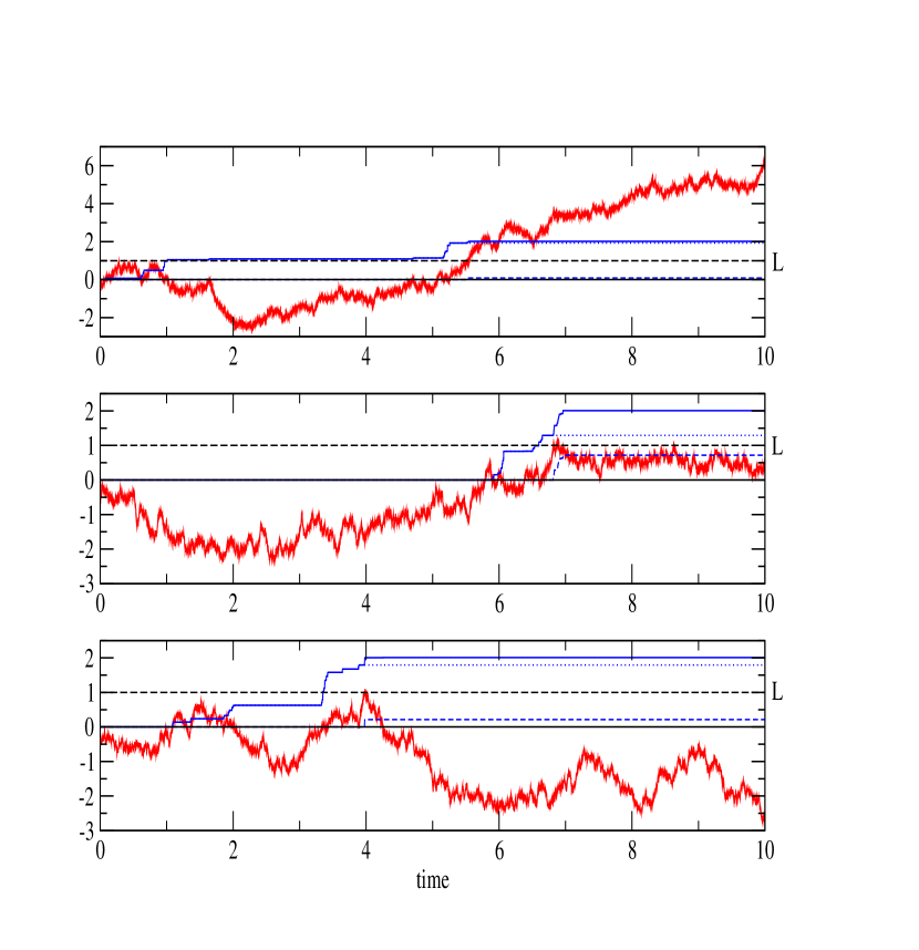
Figure 3: Red lines: Examples of realizations of diffusions conditioned to have a finite sum of local times $\Sigma_{\infty}^{*}=2$ at the infinite time horizon (see the conditioned drift of Eqs. 254, 255 and 258). For each trajectory, the associated local time $A(t)$ at $x=0$ (blue dotted line), the associated local time $B(t)$ at $x=L=1$ (blue dashed line) as well as their sum $\Sigma(t)=A(t)+B(t)$ (blue line) are shown as a function of the time $t$. All processes start at $x_{0}=-0.5$, the constant drift $\mu$ is equal to $0.5$ and the time step used in the discretization is $dt=10^{-4}$. Once the desired sum of local times $\Sigma_{\infty}^{*}=2$ is reached, there are three possibilities (i) Top figure: the process lives in the region $x\in]L=1,+\infty[$ (ii) Middle figure: the process lives in the interval $x\in]0,L=1[$ (iii) Bottom figure: the process lives in the region $x\in]-\infty,0[$

If one takes directly the limit $\tau=+\infty$ in the conditioned drift of Eq. 192, one obtains for $\Sigma<\Sigma_{\infty}^{*}$ using Eq. 250

$$\mu^{[\Sigma_{\infty}^{*}]}_{\infty}(x,\Sigma<\Sigma_{\infty}^{*})=\mu+\partial_{x}\ln\Upsilon_{\infty}(\Sigma_{T}^{*}-\Sigma|x)$$

$$=\left\{\begin{array}[]{lll}\mu&\leavevmode\nobreak\ \leavevmode\nobreak\ \mathrm{for\leavevmode\nobreak\ \leavevmode\nobreak\ }x\in]-\infty,0[\\ \mu+\partial_{x}\ln\left[\left[1-e^{\mu(L-2x)}\right]\lambda_{0}^{+}e^{-\lambda_{0}^{+}(\Sigma_{T}^{*}-\Sigma)}+\left[1+e^{\mu(L-2x)}\right]\lambda_{0}^{-}e^{-\lambda_{0}^{-}(\Sigma_{T}^{*}-\Sigma)}\right]&\leavevmode\nobreak\ \leavevmode\nobreak\ \mathrm{for\leavevmode\nobreak\ \leavevmode\nobreak\ }x\in]0,L[\\ -\mu&\leavevmode\nobreak\ \leavevmode\nobreak\ \mathrm{for\leavevmode\nobreak\ \leavevmode\nobreak\ }x\in]L,+\infty[\end{array}\right.$$ (254)

and for $\Sigma=\Sigma_{\infty}^{*}$ using Eq. 236 in the region $x\in]L,+\infty[$

$$\mu^{[\Sigma_{\infty}^{*}]}_{\infty}(x,\Sigma=\Sigma_{\infty}^{*})=\mu+\partial_{x}\ln S^{abs(0,L)}_{\infty}(x)=\mu+\partial_{x}\ln\left[1-e^{-2\mu(x-L)}\right]=\mu\coth[\mu(x-L)]\leavevmode\nobreak\ \leavevmode\nobreak\ \mathrm{for\leavevmode\nobreak\ \leavevmode\nobreak\ }x\in]L,+\infty[$$ (255)

while for the two other regions where $S^{abs(0,L)}_{\infty}(x)$ vanishes in Eq. 236, one should use the asymptotic behavior of $S^{abs(0,L)}_{\tau}(x)$ for large time $\tau$ to obtain that the conditioned drift of Eq. 192 corresponds to the taboo process on $]-\infty,0[$ and on the interval $]0,L[$ respectively. We postpone these calculations in the appendix D and state the results

$$\mu^{[\Sigma_{\infty}^{*}]}_{\infty}(x,\Sigma=\Sigma_{\infty}^{*}) =\mu+\lim_{\tau\to+\infty}\partial_{x}\ln S^{abs(0,L)}_{\tau}(x)=\left\{\begin{array}[]{lll}\frac{1}{x}&\leavevmode\nobreak\ \leavevmode\nobreak\ \mathrm{for\leavevmode\nobreak\ \leavevmode\nobreak\ }x\in]-\infty,0[\\ \frac{\pi}{L}\cot\left(\frac{\pi x}{L}\right)&\leavevmode\nobreak\ \leavevmode\nobreak\ \mathrm{for\leavevmode\nobreak\ \leavevmode\nobreak\ }x\in]0,L[\end{array}\right.$$ (258)

Figure 3 shows some realizations of this conditioned process with a drift $\mu=1/2$.

VII.5 Case $\mu>0$ : Conditioning towards the finite local times $(A_{\infty}^{*},B_{\infty}^{*})$ for the infinite horizon $T\to+\infty$

VII.5.1 Unconditioned distribution $\Pi_{\infty}(A,B|x_{0})$ of the two local times $(A,B)$ for $t=+\infty$ when starting at $x_{0}$

For the transient case $\mu>0$, the unconditioned distribution $\Pi_{\infty}(A,B|x_{0})$ of Eq. 92

$$\Pi_{\infty}(A,B|x_{0}) =\delta(A)\delta(B)S^{abs(0,L)}_{\infty}(x_{0})+\theta(A>0)\delta(B){\cal A}^{]-\infty,L[}_{\infty}(A|x_{0})+\delta(A)\theta(B>0){\cal B}^{]0,+\infty[}_{\infty}(B|x_{0})$$ (259)

$$+\theta(A>0)\theta(B>0){\cal C}_{\infty}(A,B|x_{0})$$

involves the four contributions :

(1) the first contribution $S^{abs(0,L)}_{\infty}(x_{0})$ has been given in Eq. 236

(2) the second contribution ${\cal A}^{]-\infty,L[}_{\infty}(A|x_{0})$ of Eq. 94 vanishes

$${\cal A}^{]-\infty,L[}_{\infty}(A|x_{0})=0$$ (260)

(3) the third contribution ${\cal B}^{]0,+\infty[}_{\infty}(B|x_{0})$ of Eq. 95 reads

$${\cal B}^{]0,+\infty[}_{\infty}(B|x_{0}) =e^{\mu(L-x_{0})}\left[e^{-\mu|L-x_{0}|}-e^{-\mu(L+|x_{0}|)}\right]\frac{\mu}{1-e^{-2\mu L}}e^{-\frac{\mu}{1-e^{-2\mu L}}B}$$ (264)

$$=\left\{\begin{array}[]{lll}0&\leavevmode\nobreak\ \leavevmode\nobreak\ \mathrm{for\leavevmode\nobreak\ \leavevmode\nobreak\ }x_{0}\in]-\infty,0[\\ \left[1-e^{-2\mu x_{0}}\right]\frac{\mu}{1-e^{-2\mu L}}e^{-\frac{\mu}{1-e^{-2\mu L}}B}&\leavevmode\nobreak\ \leavevmode\nobreak\ \mathrm{for\leavevmode\nobreak\ \leavevmode\nobreak\ }x_{0}\in]0,L[\\ e^{-2\mu(x_{0}-L)}\mu e^{-\frac{\mu}{1-e^{-2\mu L}}B}&\leavevmode\nobreak\ \leavevmode\nobreak\ \mathrm{for\leavevmode\nobreak\ \leavevmode\nobreak\ }x_{0}\in]L,+\infty[\end{array}\right.$$

with the normalization over $B\in]0,+\infty[$

$$\int_{0}^{+\infty}dB{\cal B}^{]0,+\infty[}_{\infty}(B|x_{0})=\left\{\begin{array}[]{lll}0&\leavevmode\nobreak\ \leavevmode\nobreak\ \mathrm{for\leavevmode\nobreak\ \leavevmode\nobreak\ }x_{0}\in]-\infty,0[\\ 1-e^{-2\mu x_{0}}&\leavevmode\nobreak\ \leavevmode\nobreak\ \mathrm{for\leavevmode\nobreak\ \leavevmode\nobreak\ }x_{0}\in]0,L[\\ e^{-2\mu(x_{0}-L)}-e^{-2\mu x_{0}}&\leavevmode\nobreak\ \leavevmode\nobreak\ \mathrm{for\leavevmode\nobreak\ \leavevmode\nobreak\ }x_{0}\in]L,+\infty[\end{array}\right.$$ (268)

(4) the fourth contribution of Eq. 97 reads

$${\cal C}_{\infty}(A,B|x_{0})=\frac{\mu^{2}}{(1-e^{-2\mu L})^{2}}e^{-\frac{\mu}{1-e^{-2\mu L}}(A+B)}e^{-\mu x_{0}}$$ (269)

$$\times\left[\left(e^{-\mu|x_{0}|}-e^{-\mu(L+|L-x_{0}|)}\right)I_{0}\left(\frac{\mu}{\sinh(\mu L)}\sqrt{AB}\right)+\left(e^{-\mu|L-x_{0}|}-e^{-\mu(L+|x_{0}|)}\right)\frac{\sqrt{B}}{\sqrt{A}}I_{1}\left(\frac{\mu}{\sinh(\mu L)}\sqrt{AB}\right)\right]$$

$$=\left\{\begin{array}[]{lll}\frac{\mu^{2}e^{-\frac{\mu}{1-e^{-2\mu L}}(A+B)}}{1-e^{-2\mu L}}I_{0}\left(\frac{\mu}{\sinh(\mu L)}\sqrt{AB}\right)&\leavevmode\nobreak\ \leavevmode\nobreak\ \mathrm{for\leavevmode\nobreak\ \leavevmode\nobreak\ }x_{0}\in]-\infty,0[\\ \frac{\mu^{2}e^{-\frac{\mu}{1-e^{-2\mu L}}(A+B)}}{(1-e^{-2\mu L})^{2}}\left[\left(e^{-2\mu x_{0}}-e^{-2\mu L}\right)I_{0}\left(\frac{\mu}{\sinh(\mu L)}\sqrt{AB}\right)+e^{-\mu L}\left(1-e^{-2\mu x_{0}}\right)\frac{\sqrt{B}}{\sqrt{A}}I_{1}\left(\frac{\mu}{\sinh(\mu L)}\sqrt{AB}\right)\right]&\leavevmode\nobreak\ \leavevmode\nobreak\ \mathrm{for\leavevmode\nobreak\ \leavevmode\nobreak\ }x_{0}\in]0,L[\\ \frac{\mu^{2}e^{-\frac{\mu}{1-e^{-2\mu L}}(A+B)}}{1-e^{-2\mu L}}e^{\mu L-2\mu x_{0}}\frac{\sqrt{B}}{\sqrt{A}}I_{1}\left(\frac{\mu}{\sinh(\mu L)}\sqrt{AB}\right)&\leavevmode\nobreak\ \leavevmode\nobreak\ \mathrm{for\leavevmode\nobreak\ \leavevmode\nobreak\ }x_{0}\in]L,+\infty[\end{array}\right.$$ (273)

with the normalization over $(A\in]0,+\infty[;B\in]0,+\infty[)$ using Eqs 365 and 368

$$\int_{0}^{+\infty}dA\int_{0}^{+\infty}dB{\cal C}_{\infty}(A,B|x_{0})=\left\{\begin{array}[]{lll}1&\leavevmode\nobreak\ \leavevmode\nobreak\ \mathrm{for\leavevmode\nobreak\ \leavevmode\nobreak\ }x_{0}\in]-\infty,0[\\ e^{-2\mu x_{0}}&\leavevmode\nobreak\ \leavevmode\nobreak\ \mathrm{for\leavevmode\nobreak\ \leavevmode\nobreak\ }x_{0}\in]0,L[\\ e^{-2\mu x_{0}}&\leavevmode\nobreak\ \leavevmode\nobreak\ \mathrm{for\leavevmode\nobreak\ \leavevmode\nobreak\ }x_{0}\in]L,+\infty[\end{array}\right.$$ (277)

VII.5.2 Conditioned drift to obtain the finite local times $(A_{\infty}^{*},B_{\infty}^{*})$ for the infinite horizon $T\to+\infty$

If one takes directly the limit $\tau=+\infty$ in the conditioned drift of Eq. 164, one obtains for $(A<A_{\infty}^{*},B<B_{\infty}^{*})$ using Eq. 269

$$\mu^{[A_{\infty}^{*},B_{\infty}^{*}]}_{\infty}(x,A<A_{\infty}^{*},B<B_{\infty}^{*})=\mu+\partial_{x}\ln{\cal C}_{\infty}(A_{\infty}^{*}-A,B_{\infty}^{*}-B|x)$$ (278)

$$=\left\{\begin{array}[]{lll}\mu&\leavevmode\nobreak\ \leavevmode\nobreak\ \mathrm{for\leavevmode\nobreak\ \leavevmode\nobreak\ }x\in]-\infty,0[\\ \mu\frac{\sqrt{B_{\infty}^{*}-B}\cosh(\mu x)I_{1}\left(\frac{\mu}{\sinh(\mu L)}\sqrt{(A_{\infty}^{*}-A)(B_{\infty}^{*}-B)}\right)-\sqrt{A_{\infty}^{*}-A}\cosh(\mu(L-x))I_{0}\left(\frac{\mu}{\sinh(\mu L)}\sqrt{(A_{\infty}^{*}-A)(B_{\infty}^{*}-B)}\right)}{\sqrt{B_{\infty}^{*}-B}\sinh(\mu x)I_{1}\left(\frac{\mu}{\sinh(\mu L)}\sqrt{(A_{\infty}^{*}-A)(B_{\infty}^{*}-B)}\right)+\sqrt{A_{\infty}^{*}-A}\sinh(\mu(L-x))I_{0}\left(\frac{\mu}{\sinh(\mu L)}\sqrt{(A_{\infty}^{*}-A)(B_{\infty}^{*}-B)}\right)}&\leavevmode\nobreak\ \leavevmode\nobreak\ \mathrm{for\leavevmode\nobreak\ \leavevmode\nobreak\ }x\in]0,L[\\ -\mu&\leavevmode\nobreak\ \leavevmode\nobreak\ \mathrm{for\leavevmode\nobreak\ \leavevmode\nobreak\ }x\in]L,+\infty[\end{array}\right.$$ (282)

and for $(A=A_{\infty}^{*},B<B_{\infty}^{*})$ using Eq. 264

$$\mu^{[A_{\infty}^{*},B_{\infty}^{*}]}_{\infty}(x,A=A_{\infty}^{*},B<B_{\infty}^{*}) =\mu+\partial_{x}\ln{\cal B}^{]0,+\infty[}_{\infty}(B_{\infty}^{*}-B|x)$$ (285)

$$=\left\{\begin{array}[]{lll}\mu+\partial_{x}\ln\left[1-e^{-2\mu x}\right]=\mu\coth(\mu x)&\leavevmode\nobreak\ \leavevmode\nobreak\ \mathrm{for\leavevmode\nobreak\ \leavevmode\nobreak\ }x\in]0,L[\\ -\mu&\leavevmode\nobreak\ \leavevmode\nobreak\ \mathrm{for\leavevmode\nobreak\ \leavevmode\nobreak\ }x\in]L,+\infty[\end{array}\right.$$

For $(A<A_{\infty}^{*},B=B_{\infty}^{*})$ where ${\cal A}^{]-\infty,L[}_{\infty}(A|x)$ vanished in Eq. (260), one should use the asymptotic behavior of ${\cal A}^{]-\infty,L[}_{\tau}(A|x)$ for large time $\tau$ to obtain that the conditioned drift has a behavior similar to the previous case, as expected

$$\mu^{[A_{\infty}^{*},B_{\infty}^{*}]}_{\infty}(x,A<A_{\infty}^{*},B=B_{\infty}^{*}) =\mu+\lim_{\tau\to+\infty}\partial_{x}\ln{\cal A}^{]-\infty,L[}_{\tau}(A_{\infty}^{*}-A|x)$$ (288)

$$=\left\{\begin{array}[]{lll}\mu&\leavevmode\nobreak\ \leavevmode\nobreak\ \mathrm{for\leavevmode\nobreak\ \leavevmode\nobreak\ }x\in]-\infty,0[\\ -\mu\coth(\mu(L-x))&\leavevmode\nobreak\ \leavevmode\nobreak\ \mathrm{for\leavevmode\nobreak\ \leavevmode\nobreak\ }x\in]0,L[\end{array}\right.$$

At last, for $(A=A_{\infty}^{*},B=B_{\infty}^{*})$, the conditioned drift involving the survival probability $S^{abs(0,L)}_{\tau}(x)$ has already been discussed above in Eqs 255 and 258. Figure 4 shows some realizations of this conditioned process with a drift $\mu=1/2$.

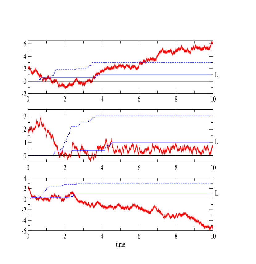
Figure 4: Red lines: Examples of realizations of diffusions conditioned to have finite local times $(A_{\infty}^{*}=3,B_{\infty}^{*}=1)$ at the infinite time horizon (see the conditioned drift of Eqs. 278, 285 and 288). For each trajectory, the associated local time $A(t)$ at $x=0$ (blue line) and the associated local time $B(t)$ at $x=L=1$ (blue dashed line) are shown as a function of the time $t$. All processes start at $x_{0}=2$, the constant drift $\mu$ is equal to $0.5$ and the time step used in the discretization is $dt=10^{-4}$. Once both the desired local times $A_{\infty}^{*}=3$ and $B_{\infty}^{*}=1$ are reached, there are three possibilities (i) Top figure: the process lives in the region $x\in]L=1,+\infty[$ (ii) Middle figure: the process lives in the interval $x\in]0,L=1[$ (iii) Bottom figure: the process lives in the region $x\in]-\infty,0[$

VIII Conclusions

In this paper, we have considered a diffusion process $X(t)$ of drift $\mu(x)$ and of diffusion coefficient $D=1/2$ in order to study the joint statistics of the two local times $A(t)=\int_{0}^{t}d\tau\delta(X(\tau))$ and $B(t)=\int_{0}^{t}d\tau\delta(X(\tau)-L)$ at positions $x=0$ and $x=L$, as well as the simpler statistics of their sum $\Sigma(t)=A(t)+B(t)$. We have discussed the asymptotic behavior for large time $t\to+\infty$ : (i) when the diffusion process $X(t)$ is transient, the two local times $[A(t);B(t)]$ remain finite random variables $[A^{*}(\infty),B^{*}(\infty)]$ and we have analyzed their limiting joint distribution ; (ii) when the diffusion process $X(t)$ is recurrent, we have described the large deviations properties of the two intensive local times $a=\frac{A(t)}{t}$ and $b=\frac{B(t)}{t}$ and of the intensive sum $\sigma=\frac{\Sigma(t)}{t}=a+b$. We have then used these properties to construct various conditioned processes $[X^{*}(t),A^{*}(t),B^{*}(t)]$ satisfying certain constraints involving the two local times, thereby generalizing our previous work [16] concerning the conditioning with respect to the single local time $A(t)$. In particular for the infinite time horizon $T\to+\infty$, we have considered the conditioning towards the finite asymptotic values $[A^{*}(\infty),B^{*}(\infty)]$ or $\Sigma^{*}(\infty)$, as well as the conditioning towards the intensive values $[a^{*},b^{*}]$ or $\sigma^{*}$, that we have compared in Appendix A with the appropriate ’canonical conditioning’ based on the generating function of the local times in the regime of large deviations. Finally, we have applied this general construction to the simplest case where the unconditioned diffusion is the Brownian motion of uniform drift $\mu$, while the comparison with the canonical conditioning is described in Appendix B.

Appendix A Canonical conditioned process $X_{p,q}^{*}(t)$ of parameters $(p,q)$

In this Appendix, we describe the properties of the canonical conditioning of parameters $(p,q)$, in order to compare with the other conditioned processes described in section VI of the main text.

A.1 Canonical conditioned process $X_{p,q}^{*}(t)$ of parameters $(p,q)$ based on the Laplace transform ${\tilde{P}}_{t,p,q}(x|x_{0})$

The canonical conditioning is based on the Laplace transform ${\tilde{P}}_{t,p,q}(x|x_{0})$ of Eq. 22 where the Laplace parameters $(p,q)$ conjugated to the two local times $A$ and $B$ are fixed. For the bridge conditioned to end at the position $x_{T}^{*}$ at the time horizon $T$, the conditioned distribution for the position $x$ at an interior time $t\in[0,T]$ reads

$$P^{[x_{T}^{*};p,q]}_{T}(x,t)=\frac{{\tilde{P}}_{T-t,p,q}(x_{T}|x){\tilde{P}}_{t,p,q}(x|x_{0})}{{\tilde{P}}_{T,p,q}(x_{T}|x_{0})}$$ (289)

The corresponding Ito dynamics for the conditioned process $X_{p,q}^{*}(t)$ of parameters $(p,q)$

$$dX_{p,q}^{*}(t)=\mu_{p,q}^{*}(X_{p,q}^{*}(t),t)dt+dB(t)$$ (290)

involves the conditioned drift

$$\mu^{[x_{T}^{*};p,q]}_{T}(x,t)=\mu(x)+\partial_{x}\ln{\tilde{P}}_{T-t,p,q}(x_{T}|x)$$ (291)

A.2 Properties of the $(p,q)$-deformed propagator ${\tilde{P}}_{t,p,q}(x|x_{0})$

The forward dynamics of the $(p,q)$-deformed propagator ${\tilde{P}}_{t,p,q}(x|x_{0})$ is given by the Feynman-Kac formula of Eq. 23

$$\partial_{t}{\tilde{P}}_{t,p,q}(x|x_{0}) =-p\delta(x){\tilde{P}}_{t,p,q}(x|x_{0})-q\delta(x-L){\tilde{P}}_{t,p,q}(x|x_{0})-\partial_{x}\left[\mu(x){\tilde{P}}_{t,p,q}(x|x_{0})\right]+\frac{1}{2}\partial_{x}^{2}{\tilde{P}}_{t,p,q}(x|x_{0})$$ (292)

A.2.1 Similarity transformation towards an hermitian quantum Hamiltonian $H_{p,q}$

The potential $U(x)$ defined via the following integration of the drift $\mu(y)$

$$U(x)\equiv-2\int_{0}^{x}dy\mu(y)$$ (293)

can be used to make the similarity transformation

$${\tilde{P}}_{t,p,q}(x|x_{0})=e^{-\frac{U(x)}{2}}\psi_{t,p,q}(x|x_{0})e^{\frac{U(x_{0})}{2}}=e^{\int_{x_{0}}^{x}dy\mu(y)}\psi_{t,p,q}(x|x_{0})$$ (294)

in order to transform the dynamics of Eq. 292 for ${\tilde{P}}_{t,p,q}(x|x_{0})$ into the Euclidean Schrödinger Equation for $\psi_{t,p,q}(x|x_{0})$

$$-\partial_{t}\psi_{t,p,q}(x|x_{0})=H_{p,q}\psi_{t,p,q}(x|x_{0})$$ (295)

where the hermitian quantum Hamiltonian $H_{p,q}$ involves two additional delta impurities of amplitudes $p$ and $q$ at positions $x=0$ and $x=L$ respectively

$$H_{p,q}=H_{0,0}+p\delta(x)+q\delta(x-L)$$ (296)

with respect to the supersymmetric Hamiltonian

$$H_{0,0}=\frac{1}{2}\left(\partial_{x}+\mu(x)\right)\left(-\partial_{x}+\mu(x)\right)=-\frac{1}{2}\partial_{x}^{2}+V(x)$$ (297)

that involves the quantum potential

$$V(x)\equiv\frac{\mu^{2}(x)}{2}+\frac{\mu^{\prime}(x)}{2}$$ (298)

A.2.2 Physical meaning of the normalizable zero-energy ground state of the supersymmetric Hamiltonian $H_{0,0}$ when it exists

Let us recall the well-known discussion :

(i) if the following integral involving the potential $U(x)$ of Eq. 293 converges

$$\int_{-\infty}^{+\infty}dxe^{-U(x)}<+\infty$$ (299)

then the quantum Hamiltonian $H_{0,0}$ has the following normalizable ground state at zero-energy $E=0$

$$\phi^{GS}_{0,0}(x)=\frac{e^{-\frac{U(x)}{2}}}{\sqrt{\int_{-\infty}^{+\infty}dye^{-U(y)}}}$$ (300)

The propagator $G_{t}(x|x_{0})={\tilde{P}}_{t,p=0,q=0}(x|x_{0})$ obtained from the similarity transformation of Eq. 294

$$G(x,t|x_{0},t_{0}) =e^{-\frac{U(x)}{2}}\psi_{t,p=0,q=0}(x|x_{0})e^{\frac{U(x_{0})}{2}}\mathop{\simeq}_{(t-t_{0})\to+\infty}e^{-\frac{U(x)}{2}}\phi^{GS}_{0,0}(x)\phi^{GS}_{0,0}(x_{0})e^{\frac{U(x_{0})}{2}}$$ (301)

$$\mathop{\simeq}_{(t-t_{0})\to+\infty}\frac{e^{-U(x)}}{\int_{-\infty}^{+\infty}dye^{-U(y)}}\equiv G_{eq}(x)$$

converges towards the Boltzmann equilibrium $G_{eq}(x)$ in the potential $U(x)$.

(ii) if the integral of Eq. 299 diverges

$$\int_{-\infty}^{+\infty}dxe^{-U(x)}=+\infty$$ (302)

then the quantum Hamiltonian $H_{0,0}$ has no bound state, and the process $X(t)$ does not converge towards an equilibrium, but it can be either transient or recurrent.

A.2.3 Propagator ${\tilde{P}}_{t,p,q}(x|x_{0})$ for large time $t$ when the quantum Hamiltonian $H_{p,q}$ has a normalizable ground-state

When the quantum Hamiltonian $H_{p,q}$ has a normalizable ground-state $\phi_{p,q}^{GS}(x)$ of energy $E_{p,q}$

$$H_{p,q}\phi_{p,q}^{GS}(x)=E_{p,q}\phi_{p,q}^{GS}(x)$$ (303)

the ground state can be chosen real and positive $\phi_{p,q}^{GS}(x)\geq 0$ with the normalization

$$\langle\phi_{p,q}^{GS}|\phi_{p}^{GS}\rangle=\int_{-\infty}^{+\infty}dx\left[\phi_{p,q}^{GS}(x)\right]^{2}=1$$ (304)

This ground-state $\phi_{p,q}^{GS}(x)$ and its energy $E_{p,q}$ determine the leading asymptotic behavior of the quantum propagator

$$\psi_{t,p,q}(x|x_{0})\mathop{\simeq}_{t\to+\infty}e^{-tE_{p,q}}\phi_{p,q}^{GS}(x)\phi_{p,q}^{GS}(x_{0})$$ (305)

The corresponding asymptotic behavior of the propagator ${\tilde{P}}_{t,p,q}(x|x_{0})$ is then given by the similarity transformation of Eq. 294

$${\tilde{P}}_{t,p,q}(x|x_{0}) =e^{-\frac{U(x)}{2}}\psi_{t,p,q}(x|x_{0})e^{\frac{U(x_{0})}{2}}$$ (306)

$$\mathop{\simeq}_{t\to+\infty}e^{-tE_{p,q}}\left[e^{-\frac{U(x)}{2}}\phi_{p,q}^{GS}(x)\right]\left[e^{\frac{U(x_{0})}{2}}\phi_{p,q}^{GS}(x_{0})\right]$$

For the further time Laplace transform ${\hat{\tilde{P}}}_{s,p,q}(x|x_{0})$ of Eq. 25, the asymptotic behavior of Eq. 306 for large $t$ means that ${\hat{\tilde{P}}}_{s,p,q}(x|x_{0})$ exists for $s\in]-E_{p,q},+\infty[$ with the following pole singularity for $s\to(-E_{p,q})^{+}$

$${\hat{\tilde{P}}}_{s,p,q}(x|x_{0})=\int_{0}^{+\infty}dte^{-st}{\tilde{P}}_{t,p,q}(x|x_{0})\mathop{\simeq}_{s\to(-E_{p,q})^{+}}\frac{\left[e^{-\frac{U(x)}{2}}\phi_{p,q}^{GS}(x)\right]\left[e^{\frac{U(x_{0})}{2}}\phi_{p,q}^{GS}(x_{0})\right]}{s+E_{p,q}}\ \ \ \$$ (307)

The comparison with the denominator of ${\hat{\tilde{P}}}_{s,p,q}(x|x_{0})$ in Eq. 31 shows that $s=-E_{p,q}$ can be found as the solution of

$$0=1+p{\hat{G}}_{s}(0|0)+q{\hat{G}}_{s}(L|L)+pq\left[{\hat{G}}_{s}(0|0){\hat{G}}_{s}(L|L)-{\hat{G}}_{s}(L|0){\hat{G}}_{s}(0|L)\right]$$ (308)

A.3 Canonical conditioning for large horizon $T$ when the Hamiltonian $H_{p,q}$ has a normalizable ground-state

When the quantum Hamiltonian $H_{p,q}$ has a normalizable ground-state $\phi_{p,q}^{GS}(x)$, the asymptotic behavior of Eq. 306 can be plugged into the the three propagators of Eq. 289 to obtain that the conditioned density at any interior time $0\ll t\ll T$

$$P^{[x_{T}^{*};p,q]}_{T}(x,t) \mathop{\simeq}_{0\ll t\ll T}\frac{e^{-E_{p,q}(T-t)}\left[e^{-\frac{U(x_{T})}{2}}\phi_{p,q}^{GS}(x_{T})\right]\left[e^{\frac{U(x)}{2}}\phi_{p,q}^{GS}(x)\right]e^{-E_{p,q}t}\left[e^{-\frac{U(x)}{2}}\phi_{p,q}^{GS}(x)\right]\left[e^{\frac{U(x_{0})}{2}}\phi_{p,q}^{GS}(x_{0})\right]}{e^{-E_{p,q}T}\left[e^{-\frac{U(x_{T})}{2}}\phi_{p,q}^{GS}(x_{T})\right]\left[e^{\frac{U(x_{0})}{2}}\phi_{p,q}^{GS}(x_{0})\right]}$$ (309)

$$=\left[\phi_{p,q}^{GS}(x)\right]^{2}\equiv P^{*}_{p,q}(x)$$

does not depend on the interior time $t$ anymore.

The corresponding conditioned drift of Eq. 291 is also independent of the interior time $t$ and reduces to

$$\mu^{[x_{T}^{*};p,q]}_{T}(x,t) \mathop{\simeq}_{0\ll t\ll T}\mu(x)+\partial_{x}\ln\left(e^{-E_{p,q}(T-t)}\left[e^{-\frac{U(x_{T})}{2}}\phi_{p,q}^{GS}(x_{T})\right]\left[e^{\frac{U(x)}{2}}\phi_{p,q}^{GS}(x)\right]\right)$$ (310)

$$=\partial_{x}\ln\left[\phi_{p,q}^{GS}(x)\right]\equiv\mu_{p,q}^{*}(x)$$

where we have used the derivative $U^{\prime}(x)=-2\mu(x)$ of the potential $U(x)$ of Eq. 293.

A.3.1 Physical meaning of this canonical conditioning when the unconditioned process $X(t)$ is recurrent

When the unconditioned process $X(t)$ is recurrent, the ground-state energy $E_{p,q}$ of the Hamiltonian $H_{p,q}$ that governs the leading exponential behavior of Eq. 306

$${\tilde{P}}_{T,p,q}(x|x_{0})\mathop{\propto}_{T\to+\infty}e^{-TE_{p,q}}$$ (311)

is directly related to the rate function $I(a,b)$ that governs the large deviations properties of the intensive local times $(a,b)$ of Eq. 12 : indeed, the saddle-point evaluation of the generating function of the two intensive local times $(a,b)$

$$\langle e^{-pTa-qTb}\rangle_{x_{0}} =\int_{0}^{+\infty}da\int_{0}^{+\infty}dbe^{-pTa-qTb}\Pi(ta,tb|x_{0})$$ (312)

$$\mathop{\simeq}_{T\to+\infty}\int_{0}^{+\infty}da\int_{0}^{+\infty}dbe^{-T\left[pa+qb+I(a,b)\right]}\mathop{\simeq}_{T\to+\infty}e^{-TE_{p,q}}$$

yields that the ground-state energy $E_{p,q}$ corresponds to the two-dimensional Legendre transform of the rate function $I(a,b)$

$$pa+qb+I(a,b) =E_{p,q}$$

$$p+\partial_{a}I(a,b) =0$$

$$q+\partial_{b}I(a,b) =0$$ (313)

while the reciprocal Legendre transform reads

$$I(a,b) =E_{p,q}-pa-qb$$

$$a =\partial_{p}E_{p,q}$$

$$b =\partial_{q}E_{p,q}$$ (314)

As a consequence, the canonical conditioning of parameters $(p,q)$ can be considered as asymptotically equivalent for large $T$ to the microcanonical conditioning towards the two intensive local times $a^{*}_{p,q}=\partial_{p}E_{p,q}$ and $b^{*}_{p,q}=\partial_{q}E_{p,q}$ corresponding to the Legendre values of Eq. 314.

These two relations have a very simple interpretation via the first-order perturbation theory for the energy $E_{p,q}$ of the ground state $\phi^{GS}_{p,q}(x)$ in quantum mechanics when the parameter $p$ is changed into $(p+\epsilon)$ or when the parameter $q$ is changed into $(q+\eta)$

$$a^{*}_{p,q} =\partial_{p}E_{p,q}=\lim_{\epsilon\to 0}\left(\frac{E_{p+\epsilon,q}-E_{p,q}}{\epsilon}\right)=\langle\phi^{GS}_{p,q}|\delta(x)|\phi^{GS}_{p,q}\rangle=\left[\phi^{GS}_{p,q}(x=0)\right]^{2}=P^{*}_{p,q}(x=0)$$

$$b^{*}_{p,q} =\partial_{q}E_{p,q}=\lim_{\eta\to 0}\left(\frac{E_{p,q+\eta}-E_{p,q}}{\eta}\right)=\langle\phi^{GS}_{p,q}|\delta(x-L)|\phi^{GS}_{p,q}\rangle=\left[\phi^{GS}_{p,q}(x=L)\right]^{2}=P^{*}_{p,q}(x=L)$$ (315)

A.3.2 Emergence of a normalizable ground-state for $H_{p,q}$ when $H_{p=0,q=0}$ has no ground state

When the quantum Hamiltonian $H_{p=0,q=0}$ has no bound state, the Hamiltonian $H_{p,q}$ of Eq. 296 can nevertheless have a normalizable bound state. Indeed, for the Laplace transform ${\hat{\tilde{P}}}_{s,p,q}(x|x_{0})$ of Eq. 25, the result of Eq. 31 shows that a new singularity can appear in ${\hat{\tilde{P}}}_{s,p,q}(x|x_{0})$ with respect to ${\hat{G}}_{s}(x|x_{0})$ when the variable $s=-E_{p,q}$ makes Eq. 308 vanish

$$0 =1+p{\hat{G}}_{s}(0|0)+q{\hat{G}}_{s}(L|L)+pq\left[{\hat{G}}_{s}(0|0){\hat{G}}_{s}(L|L)-{\hat{G}}_{s}(L|0){\hat{G}}_{s}(0|L)\right]$$ (316)

$$=\left(1+p{\hat{G}}_{s}(0|0)\right)\left(1+q{\hat{G}}_{s}(L|L)\right)-pq{\hat{G}}_{s}(0|L){\hat{G}}_{s}(L|0)$$

Let us mention the two limiting cases for the distance $L$ between the two delta impurities :

(i) if $L=0$, Eq. 316 becomes

$$0=1+(p+q){\hat{G}}_{s}(0|0)$$ (317)

and corresponds to the case of a single delta impurity of amplitude $(p+q)$ at the origin. So when $H_{0,0}$ has no bound state, a normalizable ground state state will emerge for $H_{p,q}$ if the global amplitude is strictly negative $(p+q)<0$.

(ii) if $L\to+\infty$, where it is expected that the vanishing limit ${\hat{G}}_{s}(0|L){\hat{G}}_{s}(L|0)\to 0$, Eq. 316 becomes

$$0=\left(1+p{\hat{G}}_{s}(0|0)\right)\left(1+q{\hat{G}}_{s}(L|L)\right)$$ (318)

and corresponds to two independent delta impurities of amplitude $p$ and of amplitude $q$ that become separated by the distance $L\to+\infty$. Therefore, when $H_{0,0}$ has no bound state, a normalizable ground state state will emerge for $H_{p,q}$ if at least one of the two amplitudes $p$ or $q$ is strictly negative. If the two amplitudes are strictly negative $p<0$ and $q<0$, there will be two bound states, so the ground state will correspond to the lower energy.

Let us now discuss three special cases for the parameters $(p,q)$ :

(a) In the limit $q\to+\infty$ that amounts to impose the vanishing local time $B=0$ at position $x=L$, Eq. 316 for for $s=-E_{p,q=+\infty}$ becomes

$$-p=\frac{1}{{\hat{G}}_{s}(0|0)-\frac{{\hat{G}}_{s}(0|L){\hat{G}}_{s}(L|0)}{{\hat{G}}_{s}(L|L)}}=\frac{1}{{\hat{G}}^{abs(L)}_{s}(0|0)}$$ (319)

in agreement with the pole of Eq. 37.

(b) In the limit $p\to+\infty$ that amounts to impose the vanishing local time $A=0$ at position $x=L$, Eq. 316 becomes for $s=-E_{p=+\infty,q}$

$$-q=\frac{1}{{\hat{G}}_{s}(L|L)-\frac{{\hat{G}}_{s}(L|0){\hat{G}}_{s}(0|L)}{{\hat{G}}_{s}(0|0)}}=\frac{1}{{\hat{G}}^{abs(0)}_{s}(L|L)}$$ (320)

in agreement with the pole of Eq. 44.

(c) In the special case of equal amplitudes $p=q$, Eq. 316 becomes

$$0 =\left(1+p{\hat{G}}_{s}(0|0)\right)\left(1+p{\hat{G}}_{s}(L|L)\right)-p^{2}{\hat{G}}_{s}(0|L){\hat{G}}_{s}(L|0)$$ (321)

$$=1+p\left[{\hat{G}}_{s}(0|0)+{\hat{G}}_{s}(L|L)\right]+p^{2}\Delta_{s}$$

in agreement with Eq. 124 discussed during the analysis of the sum $\Sigma=A+B$. The two roots $p^{\pm}=-\lambda_{s}^{\pm}$ correspond to two bound states, while the energy $E_{p,p}=-s$ of the ground state corresponds to $p=-\lambda_{s}^{-}$ that governs the rate function $J(\sigma)$ as discussed in Eq. 146 of the main text.

Appendix B Canonical conditioning of parameters $(p,q)$ for the case of uniform drift $\mu(x)=\mu$

In this Appendix, the canonical conditioning described in the previous Appendix is applied to the case of uniform drift $\mu(x)=\mu$, in order to compare with the other conditioned processes described in section VII of the main text.

The quantum Hamiltonian of Eq. 296 reduces to

$$H_{p,q}=-\frac{1}{2}\partial_{x}^{2}+\frac{\mu^{2}}{2}+p\delta(x)+q\delta(x-L)$$ (322)

The Hamiltonian $H_{p=0,q=0}$ has no bound state, but we will be interested in the regions of parameters $(p,q)$ where $H_{p,q}$ has a normalizable ground-state wave function $\phi^{GS}_{p,q}(x)$ (see subsection A.3.2) in order to apply the framework described in subsection A.3.

B.1 Analysis the energy $E_{p,q}$ of the normalizable ground state of $H_{p,q}$

Using ${\tilde{G}}_{s}(x|x_{0})$ of Eq. 204, Eq. 316 for $s=-E_{p,q}$ reads

$$0 =\left(1+p{\hat{G}}_{s}(0|0)\right)\left(1+q{\hat{G}}_{s}(L|L)\right)-pq{\hat{G}}_{s}(0|L){\hat{G}}_{s}(L|0)$$ (323)

$$=\left(1+\frac{p}{\kappa_{s}}\right)\left(1+\frac{q}{\kappa_{s}}\right)-pq\frac{e^{-2\kappa_{s}L}}{\kappa_{s}^{2}}$$

in terms of the parameter of Eq. 205

$$\kappa_{s}\equiv\sqrt{\mu^{2}+2s}=\sqrt{\mu^{2}-2E_{p,q}}$$ (324)

that now parametrizes the ground-state energy

$$E_{p,q}=-s=\frac{\mu^{2}-\kappa^{2}}{2}$$ (325)

In summary, once the three parameters $(p,q,L)$ are given, there will be a normalizable ground state for $H_{p,q}$ Eq. 323 that can be rewritten as

$$0=\left(1+\frac{\kappa}{p}\right)\left(1+\frac{\kappa}{q}\right)-e^{-2\kappa L}$$ (326)

that has a positive solution $\kappa_{p,q}>0$.

B.2 Analysis of the normalizable ground state wave function $\phi^{GS}_{p,q}(x)$ of $H_{p,q}$

The eigenvalue equation for the ground state wave function $\phi^{GS}_{p,q}(x)$ of energy $E_{p,q}$

$$E_{p,q}\phi^{GS}_{p,q}(x) =H_{p,q}\phi^{GS}_{p,q}(x)$$ (327)

$$=-\frac{1}{2}\partial_{x}^{2}\phi^{GS}_{p,q}(x)+\frac{\mu^{2}}{2}\phi^{GS}_{p,q}(x)+p\delta(x)\phi^{GS}_{p,q}(0)+q\delta(x-L)\phi^{GS}_{p,q}(L)$$

can be rewritten using the parametrization $E_{p,q}=\frac{\mu^{2}-\kappa_{p,q}^{2}}{2}$ of Eq. 325 as

$$0=-\partial_{x}^{2}\phi^{GS}_{p,q}(x)+\kappa_{p,q}^{2}\phi^{GS}_{p,q}(x)+2p\delta(x)\phi^{GS}_{p,q}(0)+2q\delta(x-L)\phi^{GS}_{p,q}(L)$$ (328)

The continuous solution can be decomposed into the three following regions :

(i) for the middle region $x\in[0,L]$, the wave function can be written as the linear combination involving two constants $(K^{+},K^{-})$

$$\phi^{GS}_{p,q}(x)=K^{+}e^{\kappa_{p,q}x}+K^{-}e^{\kappa_{p,q}(L-x)}\ \ {\rm for}\ \ x\in[0,L]$$ (329)

(ii) for the left region $x\in]-\infty,0]$, the wave function should be normalizable at $x\to(-\infty)$ and should be continuous with Eq. 329 at $x=0$

$$\phi^{GS}_{p,q}(x)=\phi^{GS}_{p,q}(0)e^{\kappa_{p,q}x}=(K^{+}+K^{-}e^{\kappa_{p,q}L})e^{\kappa_{p,q}x}\ \ {\rm for}\ \ x\in]-\infty,0]$$ (330)

(iii) for the right region $x\in[L,+\infty[$, the wave function should be normalizable at $x\to(+\infty)$ and should be continuous with Eq. 329 at $x=L$

$$\phi^{GS}_{p,q}(x)=\phi^{GS}_{p,q}(L)e^{-\kappa_{p,q}(x-L)}=(K^{+}e^{\kappa_{p,q}L}+K^{-})e^{-\kappa_{p,q}(x-L)}\ \ {\rm for}\ \ x\in[L,+\infty[$$ (331)

Now one needs to take into account the delta functions of Eq. 328 that impose the following discontinuities of the derivative of the wave function at $x=0$ and at $x=L$

$$2p\phi^{GS}_{p,q}(0) =\!\frac{d\phi^{GS}_{p,q}(x)}{dx}|_{x=0^{+}}\!-\!\frac{d\phi^{GS}_{p,q}(x)}{dx}|_{x=0^{-}}\!=\!\kappa_{p,q}(K^{+}-K^{-}e^{\kappa_{p,q}L})\!-\!\kappa_{p,q}(K^{+}+K^{-}e^{\kappa_{p,q}L})\!=\!-2\kappa_{p,q}K^{-}e^{\kappa_{p,q}L}$$ (332)

$$2q\phi^{GS}_{p,q}(L) =\!\frac{d\phi^{GS}_{p,q}(x)}{dx}|_{x=L^{+}}\!-\!\frac{d\phi^{GS}_{p,q}(x)}{dx}|_{x=L^{-}}\!=\!-\kappa_{p,q}(K^{+}e^{\kappa_{p,q}L}+K^{-})\!-\!\kappa_{p,q}(K^{+}e^{\kappa_{p,q}L}-K^{-})\!=\!-2\kappa_{p,q}K^{+}e^{\kappa_{p,q}L}$$

leading to the following homogeneous system for the two constants $(K^{+},K^{-})$

$$0 =p(K^{+}+K^{-}e^{\kappa_{p,q}L})+\kappa_{p,q}K^{-}e^{\kappa_{p,q}L}=pK^{+}+(p+\kappa_{p,q})e^{\kappa_{p,q}L}K^{-}$$

$$0 =q(K^{+}e^{\kappa_{p,q}L}+K^{-})+\kappa_{p,q}K^{+}e^{\kappa_{p,q}L}=(q+\kappa_{p,q})e^{\kappa_{p,q}L}K^{+}+qK^{-}$$ (333)

In order to have a non-vanishing solution, the determinant of this system should vanish

$$0=\begin{vmatrix}p&(p+\kappa_{p,q})e^{\kappa_{p,q}L}\\ (q+\kappa_{p,q})e^{\kappa_{p,q}L}&q\end{vmatrix}=pq-(p+\kappa_{p,q})(q+\kappa_{p,q})e^{2\kappa_{p,q}L}$$ (334)

i.e. one recovers Eq. 326 that determines the energy $E_{p,q}$, as it should for consistency. Therefore, Eq. 333 allows to compute the ratio

$$\frac{K^{-}}{K^{+}}=-\frac{e^{-\kappa_{p,q}L}}{1+\frac{\kappa_{p,q}}{p}}=-\left(1+\frac{\kappa_{p,q}}{q}\right)e^{\kappa_{p,q}L}$$ (335)

Finally, the global normalization of the wave function $\phi^{GS}_{p,q}(x)$

$$1=\int_{-\infty}^{+\infty}dx\left[\phi^{GS}_{p,q}(x)\right]^{2}$$ (336)

can be computed, but is not needed to evaluate the conditioned drift below.

B.3 Analysis of the conditioned drift $\mu_{p,q}^{*}(x)$

The conditioned drift of Eq. 310 can be computed from the wave function $\phi^{GS}_{p,q}(x)$ given by Eqs 329, 330 and 331 in the three regions

$$\mu_{p,q}^{*}(x) =\partial_{x}\ln\left[\phi_{p,q}^{GS}(x)\right]=\left\{\begin{array}[]{lll}\kappa_{p,q}&\leavevmode\nobreak\ \leavevmode\nobreak\ \mathrm{for\leavevmode\nobreak\ \leavevmode\nobreak\ }x\in]-\infty,0[\\ \kappa_{p,q}\frac{K^{+}e^{\kappa_{p,q}x}-K^{-}e^{-\kappa_{p,q}(x-L)}}{K^{+}e^{\kappa_{p,q}x}+K^{-}e^{-\kappa_{p,q}(x-L)}}&\leavevmode\nobreak\ \leavevmode\nobreak\ \mathrm{for\leavevmode\nobreak\ \leavevmode\nobreak\ }x\in]0,L[\\ -\kappa_{p,q}&\leavevmode\nobreak\ \leavevmode\nobreak\ \mathrm{for\leavevmode\nobreak\ \leavevmode\nobreak\ }x\in]L,+\infty[\end{array}\right.$$ (340)

that should be compared to Eqs 229, 230 and 231 of the main text.

B.3.1 Special case $q\to+\infty$ for $p\in]-\infty,0[$ corresponding to corresponding to the conditioning towards $(a_{*}>0,b_{*}=0)$

In the limit $q\to+\infty$ for $p\in]-\infty,0[$, the ground-state $\phi^{GS}_{p,q=\infty}(x)$ should vanish at $x=L$ and thus in the whole region $x\geq L$ as a consequence of Eq. 331, while the ratio of Eq. 335 reduces to

$$\frac{K^{-}}{K^{+}}\mathop{\simeq}_{q\to+\infty}-e^{\kappa_{p,\infty}L}$$ (341)

where $\kappa_{p,\infty}>0$ is the solution of Eq. 326

$$0=\left(1+\frac{\kappa_{p,\infty}}{p}\right)-e^{-2\kappa_{p,\infty}L}$$ (342)

The conditioned drift of Eq. 340 reduces to

$$\mu_{p,q=+\infty}^{*}(x)=\left\{\begin{array}[]{lll}\kappa_{p,\infty}&\leavevmode\nobreak\ \leavevmode\nobreak\ \mathrm{for\leavevmode\nobreak\ \leavevmode\nobreak\ }x\in]-\infty,0[\\ \kappa_{p,\infty}\frac{e^{\kappa_{p,\infty}x}+e^{-\kappa_{p,\infty}(x-2L)}}{e^{\kappa_{p,\infty}x}-e^{-\kappa_{p,\infty}(x-2L)}}=-\kappa_{p,\infty}\frac{\cosh[\kappa_{p,\infty}(L-x)]}{\sinh[\kappa_{p,\infty}(L-x)]}&\leavevmode\nobreak\ \leavevmode\nobreak\ \mathrm{for\leavevmode\nobreak\ \leavevmode\nobreak\ }x\in]0,L[\end{array}\right.$$ (345)

that should be compared to Eq. 221 of the main text.

B.3.2 Special case $p\to+\infty$ for $q\in]-\infty,0[$ corresponding to the conditioning towards $(a_{*}=0,b_{*}>0)$

In the limit $p\to+\infty$ for $q\in]-\infty,0[$, the ground-state $\phi^{GS}_{p=\infty,q}(x)$ should vanish at $x=0$ and thus in the whole region $x\leq 0$ as a consequence of Eq. 330, while the ratio of Eq. 335 reduces to

$$\frac{K^{-}}{K^{+}}\mathop{\simeq}_{p\to+\infty}-e^{-\kappa_{\infty,q}L}$$ (346)

where $\kappa_{\infty,q}>0$ is the solution of Eq. 326

$$0=\left(1+\frac{\kappa_{\infty,q}}{q}\right)-e^{-2\kappa_{\infty,q}L}$$ (347)

The conditioned drift of Eq. 340 reduces to

$$\mu_{p=+\infty,q}^{*}(x)=\left\{\begin{array}[]{lll}\kappa_{\infty,q}\frac{e^{\kappa_{\infty,q}x}+e^{-\kappa_{\infty,q}x}}{e^{\kappa_{\infty,q}x}-e^{-\kappa_{\infty,q}x}}=\kappa_{\infty,q}\frac{\cosh(\kappa_{\infty,q}x)}{\sinh(\kappa_{\infty,q}x)}&\leavevmode\nobreak\ \leavevmode\nobreak\ \mathrm{for\leavevmode\nobreak\ \leavevmode\nobreak\ }x\in]0,L[\\ -\kappa_{\infty,q}&\leavevmode\nobreak\ \leavevmode\nobreak\ \mathrm{for\leavevmode\nobreak\ \leavevmode\nobreak\ }x\in]L,+\infty[\end{array}\right.$$ (350)

that should be compared to Eq. 221 of the main text.

B.3.3 Special case $p=q\in]-\infty,0[$ corresponding to the conditioning towards $\sigma_{*}>0$

In the case of equal negative amplitude $p=q\in]-\infty,0[$, Eq. 326

$$0=\left(1+\frac{\kappa}{p}\right)^{2}-e^{-2\kappa L}$$ (351)

has two solutions

$$\left(1+\frac{\kappa}{p}\right)=\pm e^{-2\kappa L}$$ (352)

corresponding to two possible bound states, while the corresponding ratio of Eq. 335 takes the two possible values

$$\frac{K^{-}}{K^{+}}=-\frac{e^{-\kappa L}}{1+\frac{\kappa}{p}}=\mp 1$$ (353)

The positive ground-state wave function $\phi_{p,p}(x)$ corresponds to the ratio $\frac{K^{-}}{K^{+}}=+1$ with $\kappa_{p,p}$ solution of

$$\left(1+\frac{\kappa_{p,p}}{p}\right)=-e^{-\kappa_{p,p}L}$$ (354)

corresponding to

$$p=-\frac{\kappa_{p,p}}{1+e^{-\kappa_{p,p}L}}=-\lambda^{-}_{s}$$ (355)

where one recognizes the form $\lambda^{-}_{s}$ of Eq. 210. The other bound state associated to the negative ratio $\frac{K^{-}}{K^{+}}=-1$ corresponds to the first excited state characterized by

$$p=-\frac{\kappa_{p,p}}{1-e^{-\kappa_{p,p}L}}=-\lambda^{+}_{s}$$ (356)

where one recognizes the form of $\lambda^{+}_{s}$ of Eq. 210.

Plugging the ratio $\frac{K^{-}}{K^{+}}=+1$ for the ground state into the conditioned drift of Eq. 340 yields

$$\mu_{p,p}^{*}(x)=\left\{\begin{array}[]{lll}\kappa_{p,p}&\leavevmode\nobreak\ \leavevmode\nobreak\ \mathrm{for\leavevmode\nobreak\ \leavevmode\nobreak\ }x\in]-\infty,0[\\ \kappa_{p,p}\frac{e^{\kappa_{p,p}x}-e^{-\kappa_{p,p}(x-L)}}{e^{\kappa_{p,p}x}+e^{-\kappa_{p,p}(x-L)}}=\kappa_{p,p}\frac{\sinh\left[\kappa_{p,p}\left(x-\frac{L}{2}\right)\right]}{\cosh\left[\kappa_{p,p}\left(x-\frac{L}{2}\right)\right]}&\leavevmode\nobreak\ \leavevmode\nobreak\ \mathrm{for\leavevmode\nobreak\ \leavevmode\nobreak\ }x\in]0,L[\\ -\kappa_{p,p}&\leavevmode\nobreak\ \leavevmode\nobreak\ \mathrm{for\leavevmode\nobreak\ \leavevmode\nobreak\ }x\in]L,+\infty[\end{array}\right.$$ (360)

that should be compared to Eq. 216 of the main text.

Appendix C Explicit Laplace inversion with respect to $p$ and $q$ of the contribution ${\hat{\tilde{\cal C}}}_{s,p,q}(x|x_{0})$ of Eq. 50

In this Appendix, the goal is to compute the Laplace inversion with respect to $p$ and $q$ of the contribution ${\hat{\tilde{\cal C}}}_{s,p,q}(x|x_{0})$ of Eq. 50.

C.1 Partial fraction decomposition of ${\hat{\tilde{\cal C}}}_{s,p,q}(x|x_{0})$

To see more clearly the structure of ${\hat{\tilde{\cal C}}}_{s,p,q}(x|x_{0})$ of Eq. 50 with respect to $(p,q)$, it is convenient to introduce the shifted variables

$$P \equiv p+\frac{{\hat{G}}_{s}(L|L)}{\Delta_{s}}=p+\frac{1}{{\hat{G}}^{abs(L)}_{s}(0|0)}$$

$$Q \equiv q+\frac{{\hat{G}}_{s}(0|0)}{\Delta_{s}}=q+\frac{1}{{\hat{G}}^{abs(0)}_{s}(L|L)}$$ (361)

and the notation

$$c_{s}\equiv\frac{\sqrt{{\hat{G}}_{s}(0|L){\hat{G}}_{s}(L|0)}}{\Delta_{s}}=\ \frac{\sqrt{{\hat{G}}_{s}(0|L){\hat{G}}_{s}(L|0)}}{{\hat{G}}_{s}(0|0){\hat{G}}_{s}(L|L)-{\hat{G}}_{s}(L|0){\hat{G}}_{s}(0|L)}$$ (362)

in order to rewrite Eq. 50 as

$${\hat{\tilde{\cal C}}}_{s,p,q}(x|x_{0}) =\frac{\gamma_{s}(x|x_{0})+P\beta_{s}^{[LL]}(x|x_{0})+Q\alpha_{s}^{[00]}(x|x_{0})}{PQ-c_{s}^{2}}-\frac{\alpha_{s}^{[00]}(x|x_{0})}{P}-\frac{\beta_{s}^{[LL]}(x|x_{0})}{Q}$$ (363)

$$=\frac{\gamma_{s}(x|x_{0})}{PQ-c_{s}^{2}}+\alpha_{s}^{[00]}(x|x_{0})\left[\frac{Q}{PQ-c_{s}^{2}}-\frac{1}{P}\right]+\beta_{s}^{[LL]}(x|x_{0})\left[\frac{P}{PQ-c_{s}^{2}}-\frac{1}{Q}\right]$$

The amplitude of the first fraction

$$\gamma_{s}(x|x_{0}) =\frac{{\hat{G}}_{s}(L|L){\hat{G}}_{s}(x|0){\hat{G}}_{s}(0|x_{0})+{\hat{G}}_{s}(0|0){\hat{G}}_{s}(x|L){\hat{G}}_{s}(L|x_{0})-\left[{\hat{G}}_{s}(0|0){\hat{G}}_{s}(L|L)+{\hat{G}}_{s}(0|L){\hat{G}}_{s}(L|0)\right]\Omega_{s}(x|x_{0})}{\Delta^{2}_{s}}$$ (364)

$$=\gamma_{s}^{[L0]}(x|x_{0})+\gamma_{s}^{[0L]}(x|x_{0})$$

can be decomposed into the two terms $\gamma_{s}^{[L0]}(x|x_{0})$ and $\gamma_{s}^{[0L]}(x|x_{0})$ given in Eq. 57 of the main text.

C.2 Laplace inversion of ${\hat{\tilde{\cal C}}}_{s,p,q}(x|x_{0})$ with respect to $p$ and $q$

The Laplace inversion of the three terms of Eq. 363 involves the modified Bessel function $I_{0}(z)$ of Eq. 53 and its derivative $I_{0}^{\prime}(z)=I_{1}(z)$ of Eq. 54. The Laplace inversion of the first term of Eq. 363 is based on the identity (already used in Eq. 39 of [6])

$$\frac{1}{PQ-c^{2}}=\int_{0}^{+\infty}dxe^{-Px}\int_{0}^{+\infty}dye^{-Qy}I_{0}\left(2c\sqrt{xy}\right)$$ (365)

that can be checked by plugging the series representation of $I_{0}(z)$ of Eq. 53 into the right hand-side of Eq. 365

$$\int_{0}^{+\infty}dxe^{-Px}\int_{0}^{+\infty}dye^{-Qy}I_{0}\left(2c\sqrt{xy}\right)=\int_{0}^{+\infty}dxe^{-Px}\int_{0}^{+\infty}dye^{-Qy}\sum_{k=0}^{+\infty}\frac{\left(c\sqrt{xy}\right)^{2k}}{(k!)^{2}}$$

$$=\sum_{k=0}^{+\infty}\frac{c^{2k}}{(k!)^{2}}\int_{0}^{+\infty}dxx^{k}e^{-Px}\int_{0}^{+\infty}dyy^{k}e^{-Qy}=\sum_{k=0}^{+\infty}\frac{c^{2k}}{(k!)^{2}}\frac{(k!)^{2}}{(PQ)^{k+1}}$$

$$=\frac{1}{PQ}\sum_{k=0}^{+\infty}\left(\frac{c^{2}}{PQ}\right)^{k}=\frac{1}{PQ}\left(\frac{1}{1-\frac{c^{2}}{PQ}}\right)=\frac{1}{PQ-c^{2}}$$ (366)

The multiplication of Eq. 365 by $P$ yields via integration by parts

$$\frac{P}{PQ-c^{2}} =\int_{0}^{+\infty}dx(Pe^{-Px})\int_{0}^{+\infty}dye^{-Qy}I_{0}\left(2c\sqrt{xy}\right)=\int_{0}^{+\infty}dye^{-Qy}\int_{0}^{+\infty}dx(-\partial_{x}e^{-Px})I_{0}\left(2c\sqrt{xy}\right)$$ (367)

$$=-\int_{0}^{+\infty}dye^{-Qy}\left[e^{-Px}I_{0}\left(2c\sqrt{xy}\right)\right]_{x=0}^{x=+\infty}+\int_{0}^{+\infty}dye^{-Qy}\int_{0}^{+\infty}dxe^{-Px}\left(\partial_{x}I_{0}\left(2c\sqrt{xy}\right)\right)$$

$$=\int_{0}^{+\infty}dye^{-Qy}+\int_{0}^{+\infty}dye^{-Qy}\int_{0}^{+\infty}dxe^{-Px}\frac{c\sqrt{y}}{\sqrt{x}}I_{0}^{\prime}\left(2c\sqrt{xy}\right)$$

$$=\frac{1}{Q}+\int_{0}^{+\infty}dye^{-Qy}\int_{0}^{+\infty}dxe^{-Px}\frac{c\sqrt{y}}{\sqrt{x}}I_{1}\left(2c\sqrt{xy}\right)$$

so one obtains the identity (already used in Eq. 47 of [6])

$$\frac{P}{PQ-c^{2}}-\frac{1}{Q}=\int_{0}^{+\infty}dye^{-Qy}\int_{0}^{+\infty}dxe^{-Px}\frac{c\sqrt{y}}{\sqrt{x}}I_{1}\left(2c\sqrt{xy}\right)$$ (368)

and its analog (already used in Eq. 48 of [6])

$$\frac{Q}{PQ-c^{2}}-\frac{1}{P}=\int_{0}^{+\infty}dye^{-Qy}\int_{0}^{+\infty}dxe^{-Px}\frac{c\sqrt{x}}{\sqrt{y}}I_{1}\left(2c\sqrt{xy}\right)$$ (369)

that will allow to write the Laplace inversions of the second and third terms of Eq. 363.

If one replaces the shifted variables $(P,Q)$ of Eq. 361 in terms of the original Laplace variables $(p,q)$, the three terms of the fourth contribution ${\cal C}_{s,p,q}(x|x_{0})$ of Eq. 363

$${\hat{\tilde{\cal C}}}_{s,p,q}(x|x_{0}) ={\hat{\tilde{\cal C}}}^{[\alpha]}_{s,p,q}(x|x_{0})+{\hat{\tilde{\cal C}}}^{[\beta]}_{s,p,q}(x|x_{0})+{\hat{\tilde{\cal C}}}^{[\gamma]}_{s,p,q}(x|x_{0})$$ (370)

read

$${\hat{\tilde{\cal C}}}^{[\alpha]}_{s,p,q}(x|x_{0}) =\alpha_{s}^{[00]}(x|x_{0})\left[\frac{Q}{PQ-c_{s}^{2}}-\frac{1}{P}\right]$$

$$=\alpha_{s}^{[00]}(x|x_{0})\left[\frac{q+\frac{1}{{\hat{G}}^{abs(0)}_{s}(L|L)}}{\left(p+\frac{1}{{\hat{G}}^{abs(L)}_{s}(0|0)}\right)\left(q+\frac{1}{{\hat{G}}^{abs(0)}_{s}(L|L)}\right)-c_{s}^{2}}-\frac{1}{p+\frac{1}{{\hat{G}}^{abs(L)}_{s}(0|0)}}\right]$$

$${\hat{\tilde{\cal C}}}^{[\beta]}_{s,p,q}(x|x_{0}) =\beta_{s}^{[LL]}(x|x_{0})\left[\frac{P}{PQ-c_{s}^{2}}-\frac{1}{Q}\right]$$

$$=\beta_{s}^{[LL]}(x|x_{0})\left[\frac{p+\frac{1}{{\hat{G}}^{abs(L)}_{s}(0|0)}}{\left(p+\frac{1}{{\hat{G}}^{abs(L)}_{s}(0|0)}\right)\left(q+\frac{1}{{\hat{G}}^{abs(0)}_{s}(L|L)}\right)-c_{s}^{2}}-\frac{1}{q+\frac{1}{{\hat{G}}^{abs(0)}_{s}(L|L)}}\right]$$

$${\hat{\tilde{\cal C}}}^{[\gamma]}_{s,p,q}(x|x_{0}) =\frac{\gamma_{s}(x|x_{0})}{PQ-c_{s}^{2}}=\frac{\gamma_{s}(x|x_{0})}{\left[p+\frac{1}{{\hat{G}}^{abs(L)}_{s}(0|0)}\right]\left[q+\frac{1}{{\hat{G}}^{abs(0)}_{s}(L|L)}\right]-c_{s}^{2}}$$ (371)

So using Eqs 365, 368 and 369, the Laplace inversion with respect to $p$ and $q$ of Eq. 370 leads to Eqs 51 52 given in the main text.

C.3 Rewriting $\Omega_{s}(x|x_{0})$ in terms of $\alpha_{s}^{[00]}(x|x_{0})$, $\beta_{s}^{[LL]}(x|x_{0})$ and $\gamma_{s}(x|x_{0})$

For another computation of the main text around Eq. 127, it is useful to rewrite $\Omega_{s}(x|x_{0})$ in terms of the three functions $\alpha_{s}^{[00]}(x|x_{0})$, $\beta_{s}^{[LL]}(x|x_{0})$ and $\gamma_{s}(x|x_{0})$ by considering the special case $p=0=q$ of Eq. 50

$${\hat{\tilde{\cal C}}}_{s,p=0,q=0}(x|x_{0})=\Omega_{s}(x|x_{0})-\alpha_{s}^{[00]}(x|x_{0}){\hat{G}}^{abs(L)}_{s}(0|0)-\beta_{s}^{[LL]}(x|x_{0}){\hat{G}}^{abs(0)}_{s}(L|L)$$ (372)

and of Eq. 370

$${\hat{\tilde{\cal C}}}_{s,p=0,q=0}(x|x_{0}) ={\hat{\tilde{\cal C}}}^{[\alpha]}_{s,p=0,q=0}(x|x_{0})+{\hat{\tilde{\cal C}}}^{[\beta]}_{s,p=0,q=0}(x|x_{0})+{\hat{\tilde{\cal C}}}^{[\gamma]}_{s,p=0,q=0}(x|x_{0})$$ (373)

with Eq. 371

$${\hat{\tilde{\cal C}}}^{[\alpha]}_{s,p=0,q=0}(x|x_{0}) =\alpha_{s}^{[00]}(x|x_{0})\left[\frac{\frac{1}{{\hat{G}}^{abs(0)}_{s}(L|L)}}{\frac{1}{G^{abs(L)}_{s}(0|0){\hat{G}}^{abs(0)}_{s}(L|L)}-c_{s}^{2}}-{\hat{G}}^{abs(L)}_{s}(0|0)\right]=\alpha_{s}^{[00]}(x|x_{0})\left[\frac{\Delta_{s}}{{\hat{G}}^{abs(0)}_{s}(L|L)}-{\hat{G}}^{abs(L)}_{s}(0|0)\right]$$

$${\hat{\tilde{\cal C}}}^{[\beta]}_{s,p=0,q=0}(x|x_{0}) =\beta_{s}^{[LL]}(x|x_{0})\left[\frac{\frac{1}{{\hat{G}}^{abs(L)}_{s}(0|0)}}{\frac{1}{G^{abs(L)}_{s}(0|0){\hat{G}}^{abs(0)}_{s}(L|L)}-c_{s}^{2}}-{\hat{G}}^{abs(0)}_{s}(L|L)\right]=\beta_{s}^{[LL]}(x|x_{0})\left[\frac{\Delta_{s}}{{\hat{G}}^{abs(L)}_{s}(0|0)}-{\hat{G}}^{abs(0)}_{s}(L|L)\right]$$

$${\hat{\tilde{\cal C}}}^{[\gamma]}_{s,p=0,q=0}(x|x_{0}) =\frac{\gamma_{s}(x|x_{0})}{\frac{1}{G^{abs(L)}_{s}(0|0){\hat{G}}^{abs(0)}_{s}(L|L)}-c_{s}^{2}}=\gamma_{s}(x|x_{0})\Delta_{s}$$ (374)

The comparison between Eqs 372 and 373 374 allows to rewrite

$$\Omega_{s}(x|x_{0}) =\alpha_{s}^{[00]}(x|x_{0})\frac{\Delta_{s}}{{\hat{G}}^{abs(0)}_{s}(L|L)}+\beta_{s}^{[LL]}(x|x_{0})\frac{\Delta_{s}}{{\hat{G}}^{abs(L)}_{s}(0|0)}+\gamma_{s}(x|x_{0})\Delta_{s}$$ (375)

$$=\alpha_{s}^{[00]}(x|x_{0})G_{s}(0|0)+\beta_{s}^{[LL]}(x|x_{0})G_{s}(L|L)+\gamma_{s}(x|x_{0})\Delta_{s}$$

Appendix D Calculation of the conditioned drift $\mu^{[\Sigma_{\infty}^{*}]}_{\infty}(x,\Sigma=\Sigma_{\infty}^{*})$ when $S^{abs(0,L)}_{\tau}(x)$ vanishes for large time $\tau$

In this appendix, we provide technical details for the asymptotic analysis of the long-time of $S^{abs(0,L)}_{\tau}(x)$ when it vanishes. As described in the main text, when $S^{abs(0,L)}_{\infty}(x)$ vanishes in Eq. 236, one should use the asymptotic behavior of $S^{abs(0,L)}_{\tau}(x)$ for large time $\tau$ to obtain the conditioned drift $\mu^{[\Sigma_{\infty}^{*}]}_{\infty}(x,\Sigma=\Sigma_{\infty}^{*})$ of Eq. 192. Recall that Eq. 192

$$\mu^{[\Sigma_{\infty}^{*}]}_{\infty}(x,\Sigma=\Sigma_{\infty}^{*})=\mu(x)+\lim_{\tau\to+\infty}\partial_{x}\ln S^{abs(0,L)}_{\tau}(x)$$ (376)

where the Laplace transform of $S^{abs(0,L)}_{\tau}(x)$ is given by Eq. 79

$${\hat{S}}^{abs(0,L)}_{s}(x)=\frac{1}{s}\left[1-\frac{{\hat{G}}^{abs(L)}_{s}(0|x)}{{\hat{G}}^{abs(L)}_{s}(0|0)}-\frac{{\hat{G}}^{abs(0)}_{s}(L|x)}{{\hat{G}}^{abs(0)}_{s}(L|L)}\right]$$ (377)

where the expressions of ${\hat{G}}^{abs(L)}_{s}(x|x_{0})$ and ${\hat{G}}^{abs(0)}_{s}(x|x_{0})$ are given by Eq. 206 and Eq. 207 respectively. There are two cases depending on whether $x\in]-\infty,0[$ or $x\in]0,L[$.

D.1 Case $x\in]-\infty,0[$

When $x<0$ the expression of Eq. 377 reduces to

$${\hat{S}}^{abs(0,L)}_{s}(x)=\frac{1}{s}\left[1-e^{x(\sqrt{2s+\mu^{2}}-\mu)}\right]$$ (378)

From the inverse Laplace transform given in [107] (Eq.21a)

$$\mathcal{L}^{-1}\left\{\frac{1}{s}e^{\frac{ux}{2D}-x\sqrt{\frac{u^{2}}{4D^{2}}+\frac{s}{D}}}\right\}=\frac{1}{2}\operatorname{erfc}\left(\frac{x-u\tau}{2\sqrt{D\tau}}\right)+\frac{1}{2}e^{\frac{ux}{D}}\operatorname{erfc}\left(\frac{x+u\tau}{2\sqrt{D\tau}}\right)$$ (379)

where $\operatorname{erfc}(x)$ is the complementary error function, we immediately obtain

$${S}^{abs(0,L)}_{\tau}(x)=\frac{1}{2}\left[e^{-2x\mu}\left(-2+\operatorname{erfc}\left(\frac{x-\mu\tau}{\sqrt{2\tau}}\right)\right)+\operatorname{erfc}\left(\frac{x+\mu\tau}{\sqrt{2\tau}}\right)\right]$$ (380)

The asymptotic behavior at leading order for large time $\tau$ is given by

$$\displaystyle{S}^{abs(0,L)}_{\tau}(x)\mathop{\simeq}_{\tau\to+\infty}-\frac{1}{\mu^{2}\tau^{3/2}}\sqrt{\frac{2}{\pi}}xe^{-\frac{(x+\mu\tau)^{2}}{2\tau}}$$ (381)

and leads to

$$\mu^{[\Sigma_{\infty}^{*}]}_{\infty}(x,\Sigma=\Sigma_{\infty}^{*})=\mu+\lim_{\tau\to+\infty}\partial_{x}\ln S^{abs(0,L)}_{\tau}(x)=\frac{1}{x}-\frac{x}{\tau}=\frac{1}{x}$$ (382)

as stated in Eq. 258.

D.2 Case $x\in]0,L[$

When $x\in]0,L[$ the expression of Eq. 377 reads

$${\hat{S}}^{abs(0,L)}_{s}(x)=\frac{1}{s}\left[1+\frac{e^{-\sqrt{2s+\mu^{2}}(L+x)+\mu(L-x)}(1-e^{2\sqrt{2s+\mu^{2}}x})-e^{-x(\sqrt{2s+\mu^{2}}+\mu)}(1-e^{2\sqrt{2s+\mu^{2}}(x-L)})}{1-e^{-2\sqrt{2s+\mu^{2}}L}}\right]$$ (383)

or in a more symmetrical form

$${\hat{S}}^{abs(0,L)}_{s}(x)=\frac{1}{s}\left[1-e^{\mu(L-x)}\frac{\sinh(\sqrt{2s+\mu^{2}}x)}{\sinh(\sqrt{2s+\mu^{2}}L)}+e^{-\mu x}\frac{\sinh(\sqrt{2s+\mu^{2}}(L-x))}{\sinh(\sqrt{2s+\mu^{2}}L)}\right]$$ (384)

The inverse Laplace transform of $\sinh(\sqrt{2s+\mu^{2}}x)/(s\sinh(\sqrt{2s+\mu^{2}}L))$ can be computed exactly thanks to the residue theorem. First, there is a simple pole at $s=0$ and the residue at this point is

$$\mathop{\lim}_{s\to 0}\frac{se^{s\tau}\sinh(\sqrt{2s+\mu^{2}}x)}{s\sinh(\sqrt{2s+\mu^{2}}L)}=\frac{\sinh(\mu x)}{\sinh(\mu L)}$$ (385)

In addition, the denominator vanishes when $\sinh(\sqrt{2s+\mu^{2}}L)=0$, i.e. when $L\sqrt{2s+\mu^{2}}=n\pi i$, $n=0,\pm 1,\pm 2,...$ thus for

$$s=a_{n}=-\frac{\mu^{2}}{2}-\frac{n^{2}\pi^{2}}{2L^{2}}\leavevmode\nobreak\ \leavevmode\nobreak\ \leavevmode\nobreak\ \leavevmode\nobreak\ n=0,1,2,...$$ (386)

The residue at the point $s=a_{n}$ is

$$\mathop{\lim}_{s\to a_{n}}\frac{(s-a_{n})e^{s\tau}\sinh(\sqrt{2s+\mu^{2}}x)}{s\sinh(\sqrt{2s+\mu^{2}}L)} =\mathop{\lim}_{s\to a_{n}}\frac{(s-a_{n})}{\sinh(\sqrt{2s+\mu^{2}}L)}\mathop{\lim}_{s\to a_{n}}\frac{e^{s\tau}\sinh(\sqrt{2s+\mu^{2}}x)}{s}$$

$$=\frac{n\pi i(-1)^{n}}{L^{2}}e^{(-\frac{\mu^{2}}{2}-\frac{n^{2}\pi^{2}}{2L^{2}})\tau}\frac{i\sin\left(\frac{n\pi x}{L}\right)}{-\frac{\mu^{2}}{2}-\frac{n^{2}\pi^{2}}{2L^{2}}}$$

$$=\frac{n\pi(-1)^{n}}{L^{2}\left(\frac{\mu^{2}}{2}+\frac{n^{2}\pi^{2}}{2L^{2}}\right)}e^{-(\frac{\mu^{2}}{2}+\frac{n^{2}\pi^{2}}{2L^{2}})\tau}\sin\left(\frac{n\pi x}{L}\right)$$

Adding all the residues, we obtain

$$\mathcal{L}^{-1}\left\{\frac{\sinh(\sqrt{2s+\mu^{2}}x)}{s\sinh(\sqrt{2s+\mu^{2}}L)}\right\}=\frac{\sinh(\mu x)}{\sinh(\mu L)}+\sum_{n=1}^{\infty}\frac{n\pi(-1)^{n}}{L^{2}\left(\frac{\mu^{2}}{2}+\frac{n^{2}\pi^{2}}{2L^{2}}\right)}e^{-(\frac{\mu^{2}}{2}+\frac{n^{2}\pi^{2}}{2L^{2}})\tau}\sin\left(\frac{n\pi x}{L}\right)$$ (388)

and then

$${S}^{abs(0,L)}_{\tau}(x) =\mathcal{L}^{-1}\left\{\frac{1}{s}\left[1-e^{\mu(L-x)}\frac{\sinh(\sqrt{2s+\mu^{2}}x)}{\sinh(\sqrt{2s+\mu^{2}}L)}+e^{-\mu x}\frac{\sinh(\sqrt{2s+\mu^{2}}(L-x))}{\sinh(\sqrt{2s+\mu^{2}}L)}\right]\right\}$$

$$=1-e^{\mu(L-x)}\left[\frac{\sinh(\mu x)}{\sinh(\mu L)}+\sum_{n=1}^{\infty}\frac{n\pi(-1)^{n}}{L^{2}\left(\frac{\mu^{2}}{2}+\frac{n^{2}\pi^{2}}{2L^{2}}\right)}e^{-(\frac{\mu^{2}}{2}+\frac{n^{2}\pi^{2}}{2L^{2}})\tau}\sin\left(\frac{n\pi x}{L}\right)\right]$$

$$\leavevmode\nobreak\ \leavevmode\nobreak\ \leavevmode\nobreak\ \leavevmode\nobreak\ \leavevmode\nobreak\ +e^{-\mu x}\left[\frac{\sinh(\mu(x-L))}{\sinh(\mu L)}+\sum_{n=1}^{\infty}\frac{n\pi(-1)^{n}}{L^{2}\left(\frac{\mu^{2}}{2}+\frac{n^{2}\pi^{2}}{2L^{2}}\right)}e^{-(\frac{\mu^{2}}{2}+\frac{n^{2}\pi^{2}}{2L^{2}})\tau}\sin\left(\frac{n\pi(x-L)}{L}\right)\right]$$

$$=e^{-\mu x}\sum_{n=1}^{\infty}\left(1-e^{\mu L}(-1)^{n}\right)\frac{2n\pi}{L^{2}\mu^{2}+n^{2}\pi^{2}}e^{-(\frac{\mu^{2}}{2}+\frac{n^{2}\pi^{2}}{2L^{2}})\tau}\sin\left(\frac{n\pi x}{L}\right)$$

Keeping only the term with $n=1$, one gets the long-time asymptotic behavior

$$\displaystyle{S}^{abs(0,L)}_{\tau}(x)\mathop{\simeq}_{\tau\to+\infty}\frac{2\pi\left(1+e^{\mu L}\right)}{L^{2}\mu^{2}+\pi^{2}}e^{-(\frac{\mu^{2}}{2}+\frac{\pi^{2}}{2L^{2}})\tau}e^{-\mu x}\sin\left(\frac{\pi x}{L}\right)$$ (390)

And finally, we obtain

$$\mu^{[\Sigma_{\infty}^{*}]}_{\infty}(x,\Sigma=\Sigma_{\infty}^{*})=\mu+\lim_{\tau\to+\infty}\partial_{x}\ln S^{abs(0,L)}_{\tau}(x)=\frac{\pi}{L}\cot\left(\frac{\pi x}{L}\right)$$ (391)

as announced in Eq. 258.

References

- [1] T. Björk, ”The pedestrian’s guide to local time”, in Risk and Stochastics: Ragnar Norberg 43 (2019).
- [2] S. N. Majumdar and A. Comtet, Phys. Rev. Lett. 89, (2002) 060601.
- [3] P. C. Bressloff, Phys. Rev. E 95, 012130 (2017).
- [4] D. S. Grebenkov, Phys. Rev. Lett. 125, 078102 (2020).
- [5] D. S. Grebenkov, Phys. Rev. E 102, 032125 (2020).
- [6] D. S. Grebenkov, J. Stat. Mech. 103205 (2020).
- [7] D. S. Grebenkov, J. Phys. A.: Math. Theor. 54, 015003 (2021).
- [8] D. S. Grebenkov, 2022 J. Phys. A: Math. Theor. 55 045203.
- [9] P. C. Bressloff, 2022 J. Phys. A: Math. Theor. 55 205001.
- [10] P. C. Bressloff, 2022 J. Phys. A: Math. Theor. 55 275002.
- [11] P. C. Bressloff, arXiv:2203.04868.
- [12] D. S. Grebenkov, Phys. Rev. E 105, 054402 (2022).
- [13] D. S. Grebenkov, J. Stat. Mech. (2022) 083205.
- [14] P. C. Bressloff, 2022 Proc. R. Soc. A 478, 20220319.
- [15] P. C. Bressloff, 2022 J. Phys. A: Math. Theor. 55 415002.
- [16] A. Mazzolo and C. Monthus, J. Stat. Mech. (2022) 103207.
- [17] J.L. Doob, Bull. Soc. Math. Fr. 85, 431-48 (1957).
- [18] J.L. Doob, Classical Potential Theory and Its Probabilistic Counterpart, Springer-Verlag, New York (1984).
- [19] S. Karlin and H. Taylor, A Second Course in Stochastic Processes, Academic Press, New York (1981).
- [20] L.C.G. Rogers and D. Williams, Diffusions, Markov Processes and Martingales, vol 2, Cambridge University Press, Cambridge (2000).
- [21] A.N. Borodin, Stochastic Processes, Birkhauser, Springer International Publishing, Switzerland (2017).
- [22] S.N. Majumdar and H. Orland, J. Stat. Mech. P06039 (2015).
- [23] J.S. Horne, E.O. Garton, S.M. Krone and J.S. Lewis, Ecology 88 (9), 2354-2363 (2007).
- [24] D.C. Brody, L.P. Hughston and A. Macrina, “Beyond hazard rates: a new framework for credit-risk modelling”, in Advances in Mathematical Finance: Festschrift Volume in Honour of Dilip Madan, Birkhäuser (2007).
- [25] C. de Mulatier, E. Dumonteil, A. Rosso and A. Zoia, J. Stat. Mech. P08021 (2015).
- [26] I. Pázsit and L. Pál, Neutron Fluctuations: A Treatise on the Physics of Branching Processes, Elsevier, Oxford (2008).
- [27] S.N. Majumdar and A. Comtet, J. Stat. Phys. 119, 777-826 (2005).
- [28] K.L. Chung, Ark., Mat., 14, 155-177 (1976).
- [29] S.N. Majumdar , J. Randon-Furling, M.J. Kearney and M. Yor, J. Phys. A, Math. Theor. 41, 365005 (2008).
- [30] F.B. Knight, Trans. Amer. Soc. 73, 173–185 (1969).
- [31] R.G. Pinsky, Ann. Probab. 13 (2), 363-378 (1985).
- [32] A. Korzeniowski, Stat. Probab. Lett. 8, 229 (1989).
- [33] P. Garbaczewski, Phys. Rev. E 96 (3), 032104 (2017).
- [34] M. Adorisio, A. Pezzotta, C. de Mulatier, C. Micheletti, and A. Celani, J. Stat. Phys. 170, 79-100 (2018).
- [35] A. Mazzolo, J. Stat. Mech. P073204 (2018).
- [36] J. Grela, S.N. Majumdar and G. Schehr, J. Stat. Phys. 183, 1 (2021).
- [37] S. Karlin and S. Tavare, Stochastic Processes and their Applications 13, 249 (1982).
- [38] S. Karlin and S. Tavare, Siam J. Appl. Math. 43, 31 (1983).
- [39] H. Frydman, Comm. Stat. Stochastic Models 16, 189 (2000).
- [40] D. Steinsaltz and S.N. Evans, Trans. Amer. Math. Soc. 359, 1285 (2007).
- [41] M. Kolb and D. Steinsaltz, Annals of Probability 40, 162 (2012).
- [42] S.N. Evans and A. Hening, Stoch. Proc. Appl. 129, 1622 (2019).
- [43] Y. Chen, T.T. Georgiou and M. Pavon, Siam J. Control Optim. Vol. 60, No. 4, 2016 (2022).
- [44] A. Mazzolo and C. Monthus, J. Stat. Mech. (2022) 083207.
- [45] F. Baudoin, Stoch. Proc. Appl. 100, 109-145 (2002).
- [46] C. Larmier, A. Mazzolo and A. Zoia, J. Stat. Mech. (2019) 113208.
- [47] C. Monthus and A. Mazzolo, Phys. Rev. E 106, 044117 (2022).
- [48] A. Mazzolo and C. Monthus, 2022 J. Phys. A: Math. Theor. 55 305002.
- [49] H. Orland, J. Chem. Phys. 134, 174114 (2011).
- [50] J. Szavits-Nossan and M.R. Evans, J. Stat. Mech. P12008 (2015).
- [51] M. Delarue, P. Koehl and H. Orland, J. Chem. Phys. 147, 152703 (2017).
- [52] P. Garbaczewski and V. Stephanovich, Phys. Rev. E 99, 042126 (2019).
- [53] B. de Bruyne, S.N. Majumdar and G. Schehr, Phys. Rev. E 104, 024117 (2021).
- [54] J. Aguilar, J.W. Baron, T. Galla and R. Toral, Phys. Rev. E 105, 064138 (2022).
- [55] B. de Bruyne, S.N. Majumdar and G. Schehr, J. Phys. A: Math. Theor. 54 385004 (2021).
- [56] B. de Bruyne, S.N. Majumdar and G. Schehr, Phys. Rev. Lett. 128, 200603 (2022).
- [57] A. Mazzolo, J. Stat. Mech. P023203 (2017).
- [58] A. Mazzolo, J. Math. Phys. 58, 0953302 (2017).
- [59] B. de Bruyne, S.N. Majumdar, H. Orland and G. Schehr, J. Stat. Mech. 123204 (2021).
- [60] C. Monthus, J. Stat. Mech. (2022) 023207.
- [61] C. Giardina, J. Kurchan and L. Peliti, Phys. Rev. Lett. 96, 120603 (2006).
- [62] B. Derrida, J. Stat. Mech. P07023 (2007).
- [63] C. Giardina, J. Kurchan, V. Lecomte and J. Tailleur, J. Stat. Phys. 145, 787 (2011).
- [64] R.L. Jack and P. Sollich, The European Physical Journal Special Topics 224, 2351 (2015).
- [65] A. Lazarescu, J. Phys. A: Math. Theor. 48 503001 (2015).
- [66] A. Lazarescu, J. Phys. A: Math. Theor. 50 254004 (2017).
- [67] R.L. Jack, Eur. Phy. J. B 93, 74 (2020).
- [68] V. Lecomte, PhD Thesis (2007) ”Thermodynamique des histoires et fluctuations hors d’équilibre” Université Paris.
- [69] V. Lecomte, C. Appert-Rolland and F. van Wijland, Phys. Rev. Lett. 95, 010601 (2005).
- [70] V. Lecomte, C. Appert-Rolland and F. van Wijland, J. Stat. Phys. 127, 51 (2007).
- [71] V. Lecomte, C. Appert-Rolland and F. van Wijland, Comptes Rendus Physique 8, 609 (2007).
- [72] J.P. Garrahan, R.L. Jack, V. Lecomte, E. Pitard, K. van Duijvendijk, F. van Wijland, Phys. Rev. Lett. 98, 195702 (2007).
- [73] J.P. Garrahan, R.L. Jack, V. Lecomte, E. Pitard, K. van Duijvendijk and F. van Wijland, J. Phys. A 42, 075007 (2009).
- [74] K. van Duijvendijk, R.L. Jack and F. van Wijland, Phys. Rev. E 81, 011110 (2010).
- [75] R.L. Jack and P. Sollich, Prog. Theor. Phys. Supp. 184, 304 (2010).
- [76] D. Simon, J. Stat. Mech. (2009) P07017.
- [77] V. Popkov, G.M. Schuetz and D. Simon, J. Stat. Mech. P10007 (2010).
- [78] D. Simon, J. Stat. Phys. 142, 931 (2011).
- [79] V. Popkov and G.M. Schuetz, J. Stat. Phys 142, 627 (2011).
- [80] V. Belitsky and G.M. Schuetz, J. Stat. Phys. 152, 93 (2013).
- [81] O. Hirschberg, D. Mukamel and G.M. Schuetz, J. Stat. Mech. P11023 (2015).
- [82] G. M. Schuetz, From Particle Systems to Partial Differential Equations II, Springer Proceedings in Mathematics and Statistics Volume 129, pp 371-393, P. Goncalves and A.J. Soares (Eds.), (Springer, Cham, 2015).
- [83] R. Chétrite and H. Touchette, Phys. Rev. Lett. 111, 120601 (2013).
- [84] R. Chétrite and H. Touchette, Ann. Henri Poincaré 16, 2005 (2015).
- [85] R. Chétrite and H. Touchette, J. Stat. Mech. P12001 (2015).
- [86] R. Chétrite, HDR Thesis (2018) ”Pérégrinations sur les phénomènes aléatoires dans la nature”, Laboratoire J.A. Dieudonné, Université de Nice.
- [87] P.T. Nyawo and H. Touchette, Phys. Rev. E 94, 032101 (2016).
- [88] H. Touchette, Physica A 504, 5 (2018).
- [89] F. Angeletti and H. Touchette, Journal of Mathematical Physics 57, 023303 (2016).
-
[90]
P.T. Nyawo and H. Touchette, Europhys. Lett. 116, 50009 (2016);
P.T. Nyawo and H. Touchette, Phys. Rev. E 98, 052103 (2018). - [91] J.P. Garrahan, Physica A 504, 130 (2018).
- [92] E. Roldan and P. Vivo, Phys. Rev. E 100, 042108 (2019).
- [93] A. Lazarescu, T. Cossetto, G. Falasco and M. Esposito, J. Chem. Phys. 151, 064117 (2019).
-
[94]
B. Derrida and T. Sadhu, Journal of Statistical Physics 176, 773 (2019);
B. Derrida and T. Sadhu, Journal of Statistical Physics 177, 151 (2019). - [95] K. Proesmans and B. Derrida, J. Stat. Mech. (2019) 023201.
- [96] N. Tizon-Escamilla, V. Lecomte and E. Bertin, J. Stat. Mech. (2019) 013201.
- [97] J. du Buisson and H. Touchette, Phys. Rev. E 102, 012148 (2020).
- [98] E. Mallmin, J. du Buisson and H. Touchette, J. Phys. A: Math. Theor. 54 295001 (2021).
- [99] C. Monthus, J. Stat. Mech. (2021) 033303.
- [100] F. Carollo, J. P. Garrahan, I. Lesanovsky and C. Perez-Espigares, Phys. Rev. A 98, 010103 (2018).
- [101] F. Carollo, R.L. Jack and J.P. Garrahan, Phys. Rev. Lett. 122, 130605 (2019).
- [102] F. Carollo, J.P. Garrahan and R.L. Jack, J. Stat. Phys. 184, 13 (2021).
- [103] C. Monthus, J. Stat. Mech. (2021) 063301.
- [104] A. Lapolla, D. Hartich and A. Godec, Phys. Rev. Research 2, 043084 (2020).
- [105] L. Chabane, A. Lazarescu and G. Verley, Journal of Statistical Physics 187, 6 (2022).
- [106] L. Chabane, PhD Thesis (2021) ”From rarity to typicality : the improbable journey of a large deviation”, Université Paris-Saclay.
- [107] A. Ogata, Theory of dispersion in a granular medium, US Government Printing Office (1970), available at https://pubs.usgs.gov/pp/0411i/report.pdf