Simulation of Deflection Uncertainties on Directional Reconstructions of Muons Using PROPOSAL

Abstract

Large scale neutrino detectors and muography rely on the muon direction in the detector to infer the muon’s or parent neutrino’s origin. However, muons accumulate deflections along their propagation path prior to entering the detector, which may need to be accounted for as an additional source of uncertainty. In this paper, the deflection of muons is studied with the simulation tool PROPOSAL, which accounts for multiple scattering and deflection on stochastic interactions. Deflections along individual interactions depend on the muon energy and the interaction type, and can reach up to the order of degrees – even at TeV to PeV energies. The accumulated deflection angle can be parametrized in dependence of the final muon energy, independent of the initial muon energy. The median accumulated deflection of a propagated muon with a final energy of $500\text{\,}\frac{\mathrm{GeV}}{}$ is $\theta_{\text{acc}}=$0.10\text{\,}\frac{\mathrm{\SIUnitSymbolDegree}}{}$$ with a $99\text{\,}\frac{\mathrm{\char 37\relax}}{}$ central interval of $[$0.01\text{\,}\frac{\mathrm{\SIUnitSymbolDegree}}{}$,\,$0.39\text{\,}\frac{\mathrm{\SIUnitSymbolDegree}}{}$]$. This is on the order of magnitude of the directional resolution of present neutrino detectors. Furthermore, comparisons with the simulation tools MUSIC and Geant4 as well as two different muon deflection measurements are performed.

1 Introduction

The directional reconstruction of muons is an essential task for muography or large scale neutrino detectors such as IceCube IceCube_Instrumentation (1) or KM3NeT KM3NeT_Design (2). In both cases, the muon direction is measured at its crossing through the instrumented volume, which is then utilized to infer its origin or the origin of the parent neutrino. However, muons may propagate many kilometers prior to entering the detector while interacting with the surrounding medium. Along their propagation, muons can undergo many of thousands of interactions, depending on their energy and propagation distance. These interactions can lead to a deflection of the muon that may need to be accounted for as an additional source of uncertainty in these measurements. Current angular resolutions are above $0.1\text{\,}\frac{\mathrm{\SIUnitSymbolDegree}}{}$ for $\frac{\mathrm{TeV}}{}$ to $\frac{\mathrm{PeV}}{}$ energies in IceCube IceCube_Resolution2021 (3) and below $0.2\text{\,}\frac{\mathrm{\SIUnitSymbolDegree}}{}$ for energies greater than $10\text{\,}\frac{\mathrm{TeV}}{}$ in KM3NeT/ARCA (part of KM3NeT dedicated to search for very high-energetic neutrinos) KM3NeT_Resolution2021 (4).

To study the impact of the muon deflection on the angular resolution of current neutrino detectors, the paper is structured as follows: in section 2, the lepton propagator PROPOSAL is briefly described. In section 3, PROPOSAL koehne2013proposal (5, 6) is used to study the muon deflection per interaction. The accumulated deflection is analyzed and compared to the propagation codes MUSIC MUSIC (7, 8) and Geant4 GEANT4_standard (9, 10) and data from two experiments in section 4. The findings of this study are summarized in section 5.

2 Overview of the Simulation Tool PROPOSAL

The tool PROPOSAL koehne2013proposal (5, 6) propagates charged leptons and photons through media and is used in this paper to simulate the deflection of muons. All relevant muon interaction types as bremsstrahlung KKP_1995 (11, 12), photonuclear interaction Abramowicz_1997 (13) with shadowing ButkevichMikheyev_2002 (14), electron pair production epair_kokoulin_petrukhin (15) with corrections for the interaction with atomic electrons epair_kelner (16), ionization described by the Bethe-Bloch formula with corrections for muons Rossi (17), and the decay are provided by PROPOSAL. The interaction processes are sampled by their cross section. Since energy losses with the massless photon as secondary particle can be arbitrarily small, an energy cut is introduced to avoid an infinite number of bremsstrahlung interactions and furthermore to increase the runtime performance. The cut is applied with a minimum energy loss

$$E_{\text{loss,min}}=\min{(e_{\mathrm{cut}},E\cdot v_{\mathrm{cut}})}\,,$$ (1)

using two parameters – a total and a relative energy cut denoted as $e_{\mathrm{cut}}$ and $v_{\mathrm{cut}}$ with the energy $E$ of the particle directly before the interaction. By the introduction of this energy cut, the next significant energy loss with $E_{\mathrm{loss}}\geq E_{\text{loss,min}}$ is treated as a stochastic energy loss in the propagation. All energy losses with $E_{\mathrm{loss}}<E_{\text{loss,min}}$ between two stochastic losses are accumulated and lost continuously, denoted as continuous energy loss. The methodical uncertainties are small for a relative energy cut $v_{\mathrm{cut}}\ll 1$, however, using a small energy cut increases the runtime. Typically, a relative energy cut of $v_{\mathrm{cut}}\leq$0.05$$ is chosen which enables accurate propagations at low runtimes. The total energy cut depends on the minimum visible energy loss in the detector. It is often set to $e_{\mathrm{cut}}=$500\text{\,}\frac{\mathrm{MeV}}{}$$. The propagation process is defined by an initial muon energy $E_{\text{i}}$ and two stopping criteria – a final energy $E_{\text{f,\,min}}$ and a maximum propagation distance $d_{\text{max}}$. If the last interaction of a propagation is sampled by a stochastic interaction, the true final energy $E_{\text{f}}$ can become lower. Since muons are unstable, a decay leads to a premature stop, which is negligible for high energies.

In PROPOSAL, the deflections for stochastic interactions are parametrized by Van Ginneken in Ref. Van_Ginneken (18) with a direct calculation of the deflection in ionization using four-momentum conservation. Furthermore, there are parametrizations for stochastic deflections given in Geant4 GEANT4_standard (9, 10) for bremsstrahlung and photonuclear interaction, which are also available. To estimate the deflection along a continuous energy loss, multiple scattering described by Molière (MSM) moliere_scattering (19) and the Gaussian approximation by Highland (MSH) HIGHLAND_1975 (20) can be chosen. MSM results as a summation of elastic scatterings of one particle at another particle, called single scattering. Thus, the muon is deflected by a single angle for each continuous loss, analogous to a stochastic loss. The orientation of the deflection in the plane perpendicular to the muon direction is sampled uniformly between $0$ and $2\mathrm{\pi}$. The latest updates with a detailed description of the whole tool can be found in Ref. phd_soedingrekso (21). The stochastic deflections have been implemented in PROPOSAL recently and they are described and studied in Ref. Gutjahr_2021 (22). A publication describing the updates in PROPOSAL is in preparation alameddine_et_al (23). All simulations are done with PROPOSAL $7.3.1$.

3 Muon Deflection per Interaction

First, the stochastic deflections described by Van Ginneken Van_Ginneken (18) and implemented in PROPOSAL are investigated in combination with the two multiple scattering methods. For this purpose, $1000$ muons are propagated from $E_{\text{i}}=$1\text{\,}\frac{\mathrm{PeV}}{}$$ to $E_{\text{f,\,min}}=$1\text{\,}\frac{\mathrm{TeV}}{}$$. The deflections per interaction are presented for each interaction type and the sum over all types in Figure 1. The size of individual deflections extend over several orders of magnitude with a median of $3.9\text{\times}{10}^{-6}$ deg and a $95\text{\,}\frac{\mathrm{\char 37\relax}}{}$ central interval of $[$2.2\text{\times}{10}^{-7}$\,\text{deg},\,$1.3\text{\times}{10}^{-3}$\,\text{deg}]$. It follows that the deflections are primarily dominated by multiple scattering, except for a few outliers caused by bremsstrahlung, which allows very large energy losses and thus the largest deflections. The largest median deflection with the highest $95\text{\,}\frac{\mathrm{\char 37\relax}}{}$ interval results due to photonuclear interaction. The median propagation distance with the lower and upper $95\text{\,}\frac{\mathrm{\char 37\relax}}{}$ central interval results to $16.4_{-7.3}^{+24.6}\,$\frac{\mathrm{km}}{}$$. Detailed values for each interaction type can be found in Table 1.

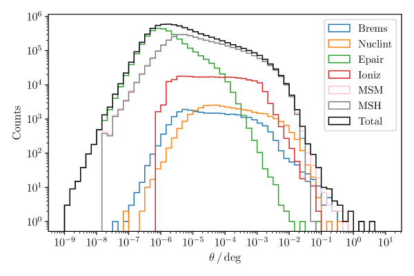
Figure 1: The muon deflection $\theta$ per interaction in degree is shown for different mechanisms. The propagation is done for $1000$ muons from $E_{\text{i}}=$1\text{\,}\frac{\mathrm{PeV}}{}$$ to $E_{\text{f,\,min}}=$1\text{\,}\frac{\mathrm{TeV}}{}$$ using $e_{\mathrm{cut}}=$500\text{\,}\frac{\mathrm{MeV}}{}$$ and $v_{\mathrm{cut}}=0.05$ in ice. The stochastic interactions are stated as Bremsstrahlung (Brems), photonuclear interaction (Nuclint), electron pair production (Epair), and ionization (Ioniz). Two simulations are done to check both multiple scattering methods Molière (MSM) and Highland (MSH). The total distribution is presented only for all stochastic processes including MSM. Since multiple scattering describes the deflection along a continuous energy loss, a single deflection occurs analogous to a stochastic deflection. Multiple scattering dominates the deflection. Details are presented in Table 1.

Table 1: The medians of deflections $\theta$ per interaction from Figure 1 are presented for each stochastic interaction type, the two multiple scattering methods, and the total distribution including MSM with the upper and lower limits of the $95\text{\,}\frac{\mathrm{\char 37\relax}}{}$ central intervals. The largest median deflection is caused by photonuclear interaction.

Brems	Nuclint	Epair	Ioniz	MSM	MSH	Total
$\theta\,/\,${10}^{-5}$\,\text{deg}$	$\theta\,/\,${10}^{-5}$\,\text{deg}$	$\theta\,/\,${10}^{-5}$\,\text{deg}$	$\theta\,/\,${10}^{-5}$\,\text{deg}$	$\theta\,/\,${10}^{-5}$\,\text{deg}$	$\theta\,/\,${10}^{-5}$\,\text{deg}$	$\theta\,/\,${10}^{-5}$\,\text{deg}$
$3.8_{-0.1}^{+297}$	$11.7_{-4.2}^{+963}$	$0.1_{-0.02}^{+4.2}$	$4.4_{-0.1}^{+181}$	$1.2_{-0.05}^{+222}$	$1.2_{-0.05}^{+225}$	$0.4_{-0.02}^{+129}$

4 Accumulated Muon Deflection

As shown in Section 3, the deflection per interaction is lower than $\sim$1\text{\,}\frac{\mathrm{\SIUnitSymbolDegree}}{}$$ in general. Since these deflections accumulate along the propagation path, the angle between the incoming and the outgoing muon direction is analyzed. This angle limits the angular resolution for neutrino source searches utilizing incoming muons, since there is no information about the muon before the detector entry.

4.1 Comparison with MUSIC and Geant4

First, the deflections in PROPOSAL are compared to the tools MUSIC and Geant4. MUSIC is a tool to simulate the propagation of muons through media like rock and water considering the same energy losses as in PROPOSAL. Also, the losses are divided into continuous and stochastic energy losses by a relative energy cut. Several cross sections, multiple scattering methods, and parametrizations for stochastic deflections are available. For these studies, the same cross section parametrizations as in PROPOSAL are chosen, except those for photonuclear interaction nulcint_bugaev_Shlepin (24, 25, 26). The stochastic deflections are also parametrized by Van Ginneken Van_Ginneken (18). The Gaussian approximation HIGHLAND_1975 (20) is set as multiple scattering. Geant4 is another common toolkit to simulate the passage of particles through matter using the same cross section parametrizations except for photonuclear interaction Borog:1975_inelastic (27). The simulation is very precise and especially made for simulations in particle detectors GEANT4_standard (9, 10).

A comparison of all three tools is shown in Figure 2 for the accumulated deflection angle $\theta_{\text{acc}}$ and the lateral displacement $x$. The propagation of $1\,000\,000$ muons with an initial energy of $E_{\mathrm{i}}=$2\text{\,}\frac{\mathrm{TeV}}{}$$ is simulated in water with a maximum propagation distance of $3\text{\,}\frac{\mathrm{km}}{}$. Four different settings are studied in PROPOSAL to compare the results with the two multiple scattering methods and the different stochastic deflection parametrizations. The deflection angles are similar in all cases. The largest displacements are exhibited by Geant4 and PROPOSAL with Molière scattering, which leads to the largest deflections and thus to a larger displacement. PROPOSAL with Highland scattering and MUSIC have less outliers, since large deflections are neglected in the Gaussian approximation HIGHLAND_1975 (20). The combination of Highland and Van Ginneken’s photonuclear interaction parametrization leads to the smallest displacement. This is due to the fact that the angle is sampled from the root mean squared angle in the exponential distribution in the parameterization for photonuclear interaction by Van Ginneken, which neglects outliers to larger angles. In general, the lateral displacements differ, although the angles are very similar in all simulations. This can be explained by the location of the deflection. If larger deflections occur sooner, they lead to further displacements during propagation, although the angle remains the same.

Detailed information are given in Table 2. The largest average deflections are obtained in Geant4 with $\overline{\theta}=$0.27\text{\,}\frac{\mathrm{\SIUnitSymbolDegree}}{}$$ and $\overline{x}=$3.3\text{\,}\frac{\mathrm{m}}{}$$, while MUSIC provides the lowest ones with $\overline{\theta}=$0.22\text{\,}\frac{\mathrm{\SIUnitSymbolDegree}}{}$$ and $\overline{x}=$2.6\text{\,}\frac{\mathrm{m}}{}$$. The results of PROPOSAL lie between these two tools. Hence, the mean values of all tools are very close to each other and therefore consistent.

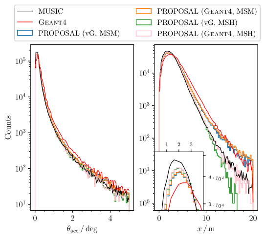
Figure 2: A comparison of the results of MUSIC, Geant4, and PROPOSAL is presented for ${10}^{6}$ muons propagated with $E_{\text{i}}=$2\text{\,}\frac{\mathrm{TeV}}{}$$ over a distance of $3\text{\,}\frac{\mathrm{km}}{}$ in water. A $v_{\mathrm{cut}}=${10}^{-3}$$ is set. In PROPOSAL, bremsstrahlung and photonuclear interaction deflections are parametrized either by Van Ginneken (vG) or as in Geant4. Both multiple scattering by Molière (MSM) and Highland (MSH) are checked. Left: The accumulated deflection $\theta_{\mathrm{acc}}$ in degree is very similar in all cases. Right: The lateral displacement $x$ in meter depends on the scattering method. MSM leads to larger distances. In the zoomed-in figure, the region around the mode of the distributions is presented. The mode of Geant4 is shifted to larger deflections. Detailed information are given in Table 2. The results for MUSIC and Geant4 are taken from Ref. comparison_MUSIC_GEANT4_2009 (8).

Table 2: The survival probability $p_{\text{s}}$ defined by the ratio of all muons that reach the propagation distance of $3\text{\,}\frac{\mathrm{km}}{}$ and the amount of muons stopping before due to large energy losses and muon decays, the mean survived muon energy $\overline{E}_{\text{f}}$, the mean scattered angle $\overline{\theta}$, and the mean displacement $\overline{x}$ are presented for all cases from Figure 2. For all means, the standard deviation is given. The largest deflection and displacement is observed in the tool Geant4, which has the lowest mean survived energy. The lower the energy, the larger the deflection.

	MUSIC	Geant4	PROPOSAL
			MSM		MSH
			vG	Geant4	vG	Geant4
$p_{\text{s}}\,/\,$\frac{\mathrm{\char 37\relax}}{}$$	77.9	79.3	77.9
$\overline{E}_{\text{f}}\,/\,$\frac{\mathrm{GeV}}{}$$	323	317	331$\pm$178
$\overline{\theta}\,/\,$\frac{\mathrm{\SIUnitSymbolDegree}}{}$$	0.22	0.27	0.24$\pm$0.45	0.24$\pm$0.45	0.22$\pm$0.35	0.22$\pm$0.35
$\overline{x}\,/\,$\frac{\mathrm{m}}{}$$	2.6	3.3	2.9$\pm$2.6	2.9$\pm$2.6	2.7$\pm$1.6	2.7$\pm$1.7

4.2 Data–MC Agreements

In the following, two comparisons are performed with measured data for different energies and media. A measurement of muon deflections in low-$Z$ materials was done by Attwood et al. attwood_2006 (28). From this it can be seen that for $Z<4$ the scattering angle is overestimated by Molière scattering in Geant4. Hence, the lower scattering in PROPOSAL leads to a better agreement especially in the region of outliers. The comparison is done in liquid $\text{H}_{2}$ with a thickness of $109\text{\,}\frac{\mathrm{mm}}{}$ and an initial particle energy of $E_{\mathrm{i}}=$199\text{\,}\frac{\mathrm{MeV}}{}$$. This energy is obtained via the energy-momentum relation of a beam momentum of $p=$168.9\text{\,}\mathrm{MeV}\text{/}\mathrm{\text{$c$}}$$ used in Ref. attwood_2006 (28). In PROPOSAL, the simulations are done with two different energy cuts $v_{\mathrm{cut}}=${10}^{-3}$$ and $v_{\mathrm{cut}}=${10}^{-5}$$, but there is no significant difference between the resulting deflections. Even though in the logarithmic figure the simulation data agree well with the measured data, it is clear from the data–MC ratio that the deviations are up to $200\text{\,}\frac{\mathrm{\char 37\relax}}{}$ in some cases. Thus, the deflections are described correctly only in a first approximation. The comparison is presented in Figure 3.

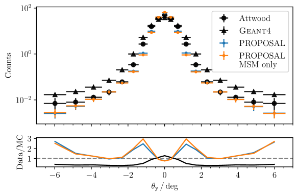
Figure 3: Muons are propagated with $E_{\mathrm{i}}=$199\text{\,}\frac{\mathrm{MeV}}{}$$ through $109\text{\,}\frac{\mathrm{mm}}{}$ of liquid $\text{H}_{2}$. Measured data of Attwood et al. and simulation data of Geant4 are taken from Ref. attwood_2006 (28). The figure presents the normalized counts in dependence of the projected scattering angle $\theta_{\mathrm{y}}$ in degree. In PROPOSAL, $100$ simulations each with ${10}^{5}$ muons are performed for two different settings using the energy cut $v_{\mathrm{cut}}=${10}^{-5}$$. The blue points present the mean of the simulations considering stochastic deflections and Molière scattering (MSM), the orange points present the mean of the simulations taking into account only Molière scattering. The uncertainties on the $x$–axis result due to the measured bin widths. The $y$–uncertainties are the standard deviations. The deflections are underestimated in PROPOSAL, except at $\theta_{\mathrm{y}}\approx$0\text{\,}\frac{\mathrm{\SIUnitSymbolDegree}}{}$$ and at $\theta_{\mathrm{y}}\approx$3\text{\,}\frac{\mathrm{\SIUnitSymbolDegree}}{}$$. At deflections $$2\text{\,}\frac{\mathrm{\SIUnitSymbolDegree}}{}$<\theta_{\mathrm{y}}<$5\text{\,}\frac{\mathrm{\SIUnitSymbolDegree}}{}$$, the result seems to be more accurate than Geant4’s. The consideration of the stochastic deflections shows no significant influence.

The second measurement of muon deflections is done for higher energetic muons of $p=$7.3\text{\,}\mathrm{GeV}\text{/}\mathrm{\text{$c$}}$$ by Akimenko et al. akimenko_1984 (29). In total, $31\,125$ muons are propagated through a $1.44\text{\,}\frac{\mathrm{cm}}{}$ thick copper layer. Again, the two energy cuts mentioned before and the effect of stochastic deflections in comparison with Molière scattering only are checked. Neither between the two energy cuts, nor when using the stochastic deflection a significant difference occurs. PROPOSAL simulates more large deflections than observed in these data. This observation differs from the comparison with Attwood, in which less higher deflections are simulated. In general, the higher muon energy leads to smaller deflections. Also simulations with Geant4 $\text{v}11.0.3$ using the default settings and the PhysicsLists QBBC and FTFP_BERT are performed. At angles larger than $0.2\text{\,}\frac{\mathrm{\SIUnitSymbolDegree}}{}$, Geant4 simulates less large deflections than PROPOSAL and less than expected in the data. Similar to the comparison with Attwood, data–MC mismatches larger than $100\text{\,}\frac{\mathrm{\char 37\relax}}{}$ are observed. There are no differences between the two PhysicsLists in the resulting deflections. The result is presented in Figure 4.

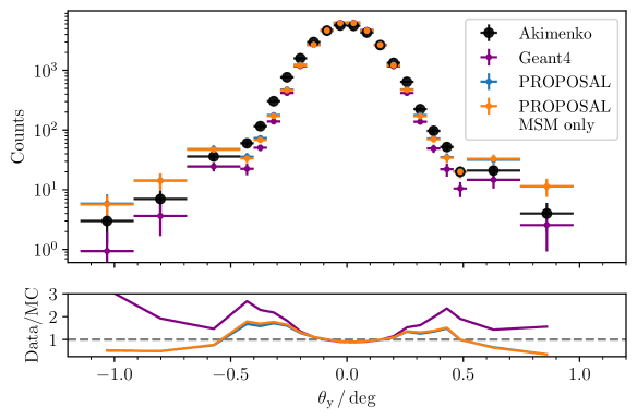
Figure 4: A comparison between two PROPOSAL simulations and measured data by Akimenko et al. akimenko_1984 (29) is presented for the normalized counts in dependence of the projected scattering angle $\theta_{\mathrm{y}}$ in degree. Deflections are simulated with Geant4 $\text{v}11.0.3$ as well. $100$ simulations each with $31\,125$ muons with $E_{\mathrm{i}}=$7.301\text{\,}\frac{\mathrm{GeV}}{}$$ are propagated through a $1.44\text{\,}\frac{\mathrm{cm}}{}$ copper layer. In PROPOSAL the energy cut $v_{\mathrm{cut}}=${10}^{-5}$$ is used. The blue points present the mean of the simulation considering stochastic deflections and Molière scattering (MSM), the orange points present the mean of the simulation taking into account only Molière scattering. The uncertainties on the $x$–axis result due to the measured bin widths. The $y$–uncertainties are the standard deviations for PROPOSAL and the Poisson errors with $\sqrt{N}$ for Akimenko, with $N$ as number of counts. More large deflections are simulated by PROPOSAL. Considering stochastic deflections has no significant impact.

4.3 Muon Deflection Impact on Angular Resolutions

For neutrino source searches based on muons entering the detector, it is important to study the impact of the muon deflection on the angular resolution to estimate whether or not this needs to be taken into account as an additional source of uncertainty. For this purpose, four different initial energies from $E_{\text{i}}=$10\text{\,}\frac{\mathrm{TeV}}{}$$ to $E_{\text{i}}=$10\text{\,}\frac{\mathrm{PeV}}{}$$ are used and the final energy is set to $E_{\text{f,\,min}}\geq$1\text{\,}\frac{\mathrm{GeV}}{}$$ with $E_{\text{f,\,min}}<E_{\text{i}}$ for each simulation. This energy range covers the muon energies typically measured in neutrino experiments. In total $44$ simulations are performed. To compare the results of these simulations, the medians of the deflection distributions with a $99\text{\,}\frac{\mathrm{\char 37\relax}}{}$ central interval are presented in Figure 5. The lower the final muon energy, the larger the accumulated deflection. For energies $E_{\text{f}}=$1\text{\,}\frac{\mathrm{PeV}}{}$$, the median deflection is ${10}^{-4}$ deg. For energies $E_{\text{f}}=$100\text{\,}\frac{\mathrm{GeV}}{}$$, angles larger than $1\text{\,}\frac{\mathrm{\SIUnitSymbolDegree}}{}$ are possible. For energies $E_{\text{f}}\leq$1\text{\,}\frac{\mathrm{TeV}}{}$$, there is a small overlap of the deflection with the angular resolution of KM3NeT/ARCA KM3NeT_Resolution2021 (4, 30). At low energies of $E_{\mathrm{f}}=$5\text{\,}\frac{\mathrm{GeV}}{}$$, the upper limit of the deflections affects the resolution of SuperKamiokande SuperKamiokande_Resolution2008 (31). The kinematic scattering angle between the incident neutrino and the produced muon is larger than the deflection in the presented region from $60\text{\,}\frac{\mathrm{GeV}}{}$ to $200\text{\,}\frac{\mathrm{TeV}}{}$. For energies below $2\text{\,}\frac{\mathrm{TeV}}{}$, the muon deflections are of the same order of magnitude as the kinematic angle and thus become increasingly relevant. Here it must be noted that the kinematic angle and the resolution of ARCA in Ref. KM3NeT_Resolution2021 (4) as well as the resolutions of ORCA (part of KM3NeT optimized to study atmospheric neutrinos in the $\frac{\mathrm{GeV}}{}$ energy range) ORCA_Resolution2021 (32) and ANTARES ANTARES_Resolution2019 (33) are presented in dependence of the neutrino energy. Hence, a rescaling to the muon energy is applied using the average energy transfer of the neutrino to the nucleus GANDHI199681 (34). This shifts the curves to lower energies. Since all of these simulations are done in ice, the same simulations are done in water to compare the results for water-based experiments. The deviations of the medians are less than $1\text{\,}\frac{\mathrm{\char 37\relax}}{}$ for all energies and therefore not shown. The accumulated deflections and also the propagated distances of Figure 5 are presented in Table 3. Muons are able to propagate various distances for a fixed final muon energy depending on the stochasticity of the energy losses.

Note that the distribution of deflection angles at a given final energy $E_{\mathrm{f}}$ in Figure 5 overlap for differing initial energies. This result indicates that the total deflection of a muon primarily depends on the final muon energy. The initial muon energy is nearly irrelevant. Hence, the reconstructed muon energy in a detector can be used to estimate the deflection. For this purpose, a polynomial of degree three as

$$f(x)=a\cdot x^{3}+b\cdot x^{2}+c\cdot x+d\,,$$ (2)

can be used with the parameters

$$a= +0.0176\pm 0.0018\,, c= +0.0929\pm 0.0527\,,$$

$$b= -0.2328\pm 0.0185\,, d= +0.0726\pm 0.0404\,,$$

in the logarithmic space via

$$g(x)= 10^{f(x)}\,, x= \log_{10}\left(\frac{E_{\text{f}}}{$\frac{\mathrm{GeV}}{}$}\right)\,.$$ (3)

In general, the function $f(x)$ in Eq. (2) describes the median deflection of a muon after a propagated distance in ice for a given, respectively measured energy to estimate the deflection before the detector entry. This equation is valid for muon energies between $1\text{\,}\frac{\mathrm{GeV}}{}$ and $50\text{\,}\frac{\mathrm{PeV}}{}$. Basically, it should be mentioned here that the data–MC comparisons shown earlier are for energies of $E_{\mathrm{i}}=$199\text{\,}\frac{\mathrm{MeV}}{}$$ and $E_{\mathrm{i}}=$7.3\text{\,}\frac{\mathrm{GeV}}{}$$, which are much lower than the energies in these simulations.

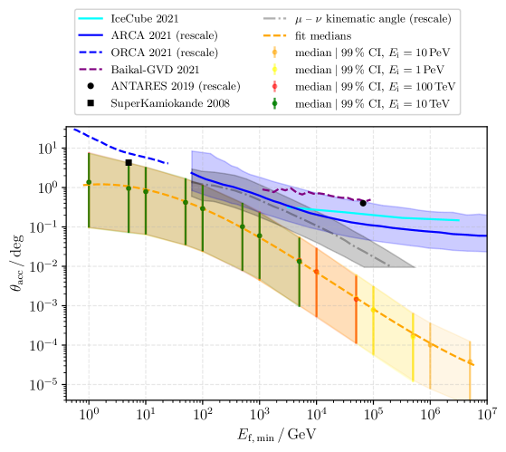
Figure 5: The median of the accumulated deflection $\theta_{\text{acc}}$ in degree with a $99\text{\,}\frac{\mathrm{\char 37\relax}}{}$ central interval is shown for four different initial energies $E_{\text{i}}$. Each data set includes more than $50\,000$ events with the requirement that the true final muon energy $E_{\text{f}}$ is at most $10\text{\,}\frac{\mathrm{\char 37\relax}}{}$ below the set final energy $E_{\text{f,\,min}}$, $E_{\text{f}}>E_{\text{f,\,min}}\cdot 0.9$. The energy cuts are $e_{\mathrm{cut}}=$500\text{\,}\frac{\mathrm{MeV}}{}$$ and $v_{\mathrm{cut}}=0.05$, and Molière scattering is chosen. Simulations are performed in ice, the deviations of the medians in a water-based simulation are smaller than $1\text{\,}\frac{\mathrm{\char 37\relax}}{}$. Since the medians overlap for different initial energies, there is no strong impact of the initial energy on the median deflection. These medians can be fit by a third degree polynomial in the log-space as shown in Eq. (2). The kinematic angle between the muon and neutrino is taken from Ref. KM3NeT_Resolution2021 (4). Since the kinematic angle and the angular resolution of ARCA taken from Ref. KM3NeT_Resolution2021 (4) are presented in dependence of the neutrino energy as well as the resolutions of ORCA ORCA_Resolution2021 (32) and ANTARES ANTARES_Resolution2019 (33), a rescaling to the muon energy is performed using the average energy transfer to the nucleus GANDHI199681 (34). For energies $E_{\text{f}}\leq$1\text{\,}\frac{\mathrm{TeV}}{}$$, there is a minimal influence of the deflection on the angular resolution of ARCA and at $E_{\mathrm{f}}=$5\text{\,}\frac{\mathrm{GeV}}{}$$ the upper limit of the deflections affects the resolution of SuperKamiokande SuperKamiokande_Resolution2008 (31). The resolutions shown by IceCube IceCube_Resolution2021 (3), ORCA, Baikal Baikal_Resolution2021 (35) and ANTARES are not impacted, but no uncertainty bands are given for these either. The exact values and the propagated distances are presented in Table 3.

To analyze the impact of the propagation distance on the muon deflection, another simulation is done. This time, the initial energies are not fixed and sampled from an atmospheric muon flux at sea level by gaisser1990 (36) with a weighting of $E^{3.7}$ for energies from $10\text{\,}\frac{\mathrm{GeV}}{}$ to $1\text{\times}{10}^{10}\text{\,}\frac{\mathrm{GeV}}{}$. The final energies are sampled similar. The resulting deflections are presented in Figure 6. From this follows, that the median deflection is not impacted by the propagation distance, if the initial muon energy is unknown. This is a realistic scenario for example for a neutrino telescope, since the only known value is the reconstructed muon energy at the detector entry. There are no information about the initial energy and the propagation distance. Finally, the muon deflection can be estimated only by the reconstructed muon energy.

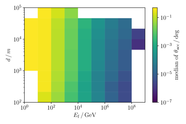
Figure 6: The median of the accumulated deflection $\theta_{\mathrm{acc}}$ is presented in degree as a function of the final muon energy $E_{\mathrm{f}}$ and the propagation distance $d$. The result is presented for $50\,370$ muons for a propagation through ice. An energy cut of $v_{\mathrm{cut}}=$1\text{\times}{10}^{-3}$$, MSM and the deflection parametrizations of vG are used. The initial energies are not fixed. The muon deflection depends primarily only on the final muon energy. Even the propagation distance is negligible if the initial muon energy is unknown.

4.4 Relevance for Muography

Muography is a technique to study the inside of structures with a wide field of applications such as the monitoring of volcanic activity and many more. For this, the atmospheric muon flux is measured with a detector located below or even behind the object, which is visualized. The muon flux count rates then depend on the densities of the materials, the higher the density, the stronger the attenuation. Based on this, conclusions can be drawn about materials and cavities in the respective object. Sufficient statistics in reasonable time are obtained for muons in the $\frac{\mathrm{GeV}}{}$ energy range muography_2019 (37).

Angular resolutions of these detectors are below $0.6\text{\,}\frac{\mathrm{\SIUnitSymbolDegree}}{}$, which is on the order of magnitude of the muon deflection at $\frac{\mathrm{GeV}}{}$ muon energies. Multiple scattering of muon deflection in several media is also studied in muography_2019 (37, 38). The resulting deflections are about $1\text{\,}\frac{\mathrm{\SIUnitSymbolDegree}}{}$, similar to the deflections expected with PROPOSAL in water and ice. Hence, the scattering of muons can be a limiting factor for the angular resolution in muography at energies of a few $\frac{\mathrm{GeV}}{}$.

5 Conclusion

Stochastic deflection, recently implemented in PROPOSAL 7.3.0, is used to study the muon deflection per interaction. The deflection is dominated by multiple scattering except for a few stochastic outliers by bremsstrahlung. These angles are lower than $\sim$1\text{\,}\frac{\mathrm{\SIUnitSymbolDegree}}{}$$.

The results of PROPOSAL are compared with the common tools MUSIC and Geant4 and they are in good agreement. In low-$Z$ materials, the region of outlier deflections fits the measured data better with PROPOSAL, than Geant4. A second data comparison points out that PROPOSAL simulates more large deflections at higher muon energies and less at lower energies. In the data–MC ratio deviations up to a factor of $3$ are observed. This points out that still improvements are required in the deflection parameterizations and in the multiple scattering, respectively. Since the presented measurements of the muon deflection are based on muon energies lower $10\text{\,}\frac{\mathrm{GeV}}{}$, deflection measurements of muons with energies up to $\frac{\mathrm{TeV}}{}$ or even higher are required to validate the results at higher energies.

The median accumulated deflection depends primarily on the final muon energy, which can be interpreted as the muon energy at detector entry in neutrino telescopes or other muon detectors. The outcome is fit by a polynomial and can be used for a theoretical estimation of the muon deflection in water and ice. Since the result can be interpreted as the deflection before the detector entry, it defines a lower limit on the directional resolution. At energies lower $1\text{\,}\frac{\mathrm{TeV}}{}$, there is potentially a small impact of the muon deflection on the angular resolution of KM3NeT.

Table 3: The median values for the accumulated deflection $\theta_{\mathrm{acc}}$ in degree and the propagated distances $d$ in meter are presented for Figure 5. The upper and lower values indicate the upper und lower $99\text{\,}\frac{\mathrm{\char 37\relax}}{}$ intervals around the median. It turns out that the median deflection depends primarily only on the final muon energy $E_{\mathrm{f,\,min}}$.

	$E_{\mathrm{i}}=$10\text{\,}\frac{\mathrm{PeV}}{}$$		$E_{\mathrm{i}}=$1\text{\,}\frac{\mathrm{PeV}}{}$$		$E_{\mathrm{i}}=$100\text{\,}\frac{\mathrm{TeV}}{}$$		$E_{\mathrm{i}}=$10\text{\,}\frac{\mathrm{TeV}}{}$$
$E_{\mathrm{f,\,min}}\,/\,$\frac{\mathrm{GeV}}{}$$	$\theta_{\text{acc}}\,/\,$\frac{\mathrm{\SIUnitSymbolDegree}}{}$$	$d\,/\,$\frac{\mathrm{km}}{}$$	$\theta_{\text{acc}}\,/\,$\frac{\mathrm{\SIUnitSymbolDegree}}{}$$	$d\,/\,$\frac{\mathrm{km}}{}$$	$\theta_{\text{acc}}\,/\,$\frac{\mathrm{\SIUnitSymbolDegree}}{}$$	$d\,/\,$\frac{\mathrm{km}}{}$$	$\theta_{\text{acc}}\,/\,$\frac{\mathrm{\SIUnitSymbolDegree}}{}$$	$d\,/\,$\frac{\mathrm{km}}{}$$
$1$	$1.36_{0.10}^{7.33}$	$23.7_{9.10}^{37.8}$	$1.36_{0.09}^{7.38}$	$18.7_{6.05}^{30.4}$	$1.37_{0.10}^{7.75}$	$13.5_{3.60}^{21.9}$	$1.37_{0.10}^{7.47}$	$7.91_{1.65}^{12.2}$
$5$	$9.48_{0.74}^{41.9}\times 10^{-1}$	$23.8_{8.99}^{37.6}$	$9.53_{0.74}^{42.3}\times 10^{-1}$	$18.7_{5.97}^{30.3}$	$9.52_{0.74}^{42.7}\times 10^{-1}$	$13.4_{3.48}^{21.9}$	$9.50_{0.71}^{42.3}\times 10^{-1}$	$7.89_{1.63}^{12.2}$
$10$	$7.88_{0.64}^{33.1}\times 10^{-1}$	$23.8_{9.15}^{37.8}$	$7.93_{0.63}^{32.0}\times 10^{-1}$	$18.7_{6.19}^{30.1}$	$7.89_{0.65}^{33.0}\times 10^{-1}$	$13.4_{3.62}^{21.9}$	$7.85_{0.65}^{33.0}\times 10^{-1}$	$7.84_{1.58}^{12.1}$
$50$	$4.19_{0.34}^{16.5}\times 10^{-1}$	$23.7_{9.10}^{37.6}$	$4.21_{0.34}^{16.8}\times 10^{-1}$	$18.5_{6.08}^{30.0}$	$4.18_{0.35}^{16.5}\times 10^{-1}$	$13.2_{3.58}^{21.7}$	$4.20_{0.35}^{17.2}\times 10^{-1}$	$7.72_{1.48}^{12.0}$
$100$	$2.95_{0.24}^{11.7}\times 10^{-1}$	$23.5_{9.00}^{37.2}$	$2.92_{0.23}^{11.0}\times 10^{-1}$	$18.4_{6.02}^{29.9}$	$2.91_{0.24}^{11.8}\times 10^{-1}$	$13.1_{3.54}^{21.6}$	$2.92_{2.44}^{11.5}\times 10^{-1}$	$7.55_{1.46}^{11.8}$
$500$	$1.01_{0.08}^{3.92}\times 10^{-1}$	$22.6_{8.33}^{36.3}$	$1.02_{0.08}^{3.86}\times 10^{-1}$	$17.5_{5.44}^{28.9}$	$1.02_{0.07}^{4.06}\times 10^{-1}$	$12.2_{2.87}^{20.5}$	$1.02_{0.08}^{4.09}\times 10^{-1}$	$6.68_{1.01}^{10.7}$
$1000$	$5.90_{0.44}^{22.7}\times 10^{-2}$	$21.8_{7.65}^{35.4}$	$5.92_{0.44}^{2.29}\times 10^{-2}$	$16.8_{4.85}^{27.9}$	$5.92_{0.44}^{24.7}\times 10^{-2}$	$11.5_{2.38}^{19.4}$	$6.00_{0.48}^{23.1}\times 10^{-2}$	$5.86_{0.78}^{9.54}$
$5000$	$1.41_{0.10}^{5.42}\times 10^{-2}$	$19.0_{6.16}^{31.6}$	$1.42_{0.10}^{5.78}\times 10^{-2}$	$13.9_{3.38}^{24.0}$	$1.42_{0.10}^{5.54}\times 10^{-2}$	$8.58_{1.20}^{15.2}$	$1.33_{0.09}^{5.30}\times 10^{-2}$	$2.54_{0.17}^{4.28}$
$10\,000$	$7.33_{0.55}^{28.3}\times 10^{-3}$	$17.4_{5.11}^{29.4}$	$7.36_{0.52}^{28.8}\times 10^{-3}$	$12.4_{2.60}^{21.8}$	$7.37_{0.51}^{29.5}\times 10^{-3}$	$7.03_{0.76}^{12.7}$	—	—
$50\,000$	$1.53_{0.11}^{6.23}\times 10^{-3}$	$13.6_{3.25}^{24.0}$	$1.53_{0.11}^{6.01}\times 10^{-3}$	$8.56_{1.16}^{15.7}$	$1.46_{0.11}^{5.70}\times 10^{-3}$	$2.75_{0.17}^{5.02}$	—	—
$100\,000$	$7.80_{0.58}^{31.4}\times 10^{-4}$	$11.9_{2.49}^{21.4}$	$7.90_{0.55}^{31.0}\times 10^{-4}$	$6.89_{0.73}^{12.8}$	—	—	—	—
$500\,000$	$1.75_{0.13}^{6.53}\times 10^{-4}$	$8.16_{1.11}^{15.3}$	$1.58_{0.12}^{6.14}\times 10^{-4}$	$2.67_{0.16}^{5.04}$	—	—	—	—
$1\,000\,000$	$1.01_{0.08}^{3.65}\times 10^{-4}$	$6.54_{0.64}^{12.4}$	—	—	—	—	—	—
$50\,000\,000$	$3.81_{0.30}^{12.5}\times 10^{-5}$	$2.55_{0.13}^{4.96}$	—	—	—	—	—	—

References

- (1) M.. Aartsen “The IceCube Neutrino Observatory: Instrumentation and Online Systems” In JINST 12, 2017, pp. P03012 DOI: 10.1088/1748-0221/12/03/P03012
- (2) P. Bagley “KM3NeT: Technical Design Report for a Deep-Sea Research Infrastructure in the Mediterranean Sea Incorporating a Very Large Volume Neutrino Telescope”, 2010
- (3) R. Abbasi “A muon-track reconstruction exploiting stochastic losses for large-scale Cherenkov detectors” In JINST 16.08, 2021, pp. P08034 DOI: 10.1088/1748-0221/16/08/P08034
- (4) B. Caiffi et al. “Sensitivity estimates for diffuse, point-like, and extended neutrino sources with KM3NeT/ ARCA” In JINST 16.09, 2021, pp. C09030 DOI: 10.1088/1748-0221/16/09/c09030
- (5) J.-H. Koehne et al. “PROPOSAL: A tool for propagation of charged leptons” In Comput. Phys. Commun. 184.9, 2013, pp. 2070–2090 DOI: 10.1016/j.cpc.2013.04.001
- (6) M. Dunsch et al. “Recent Improvements for the Lepton Propagator PROPOSAL” In Comput. Phys. Commun. 242, 2019, pp. 132–144 DOI: 10.1016/j.cpc.2019.03.021
- (7) P. Antonioli et al. “A three-dimensional code for muon propagation through the rock: MUSIC” In Astropart. Phys. 7, 1997, pp. 357–368 DOI: 10.1016/S0927-6505(97)00035-2
- (8) V.. Kudryavtsev “Muon simulation codes MUSIC and MUSUN for underground physics” In Comput. Phys Commun. 180.3, 2009, pp. 339–346 DOI: 10.1016/j.cpc.2008.10.013
- (9) S. al “GEANT4 – a simulation toolkit” In Nucl. Instrum. Meth. A 506.3, 2003, pp. 250–303 DOI: 10.1016/S0168-9002(03)01368-8
- (10) Geant4 Collaboration “Geant4 Physics Reference Manual”, 2021 URL: geant4.web.cern.ch
- (11) S.. Kelner, R.. Kokoulin and A.. Petrukhin “About Cross Section for High-Energy Muon Bremsstrahlung”, Preprint MEPhI 024-95, 1995 URL: https://cds.cern.ch/record/288828
- (12) S.. Kelner, R.. Kokoulin and A.. Petrukhin “Bremsstrahlung from muons scattered by atomic electrons” In Phys. At. Nucl. 60.4, 1997, pp. 576–583
- (13) H. Abramowicz and A. Levy “The ALLM Parametrization of - An Update”, 1997 arXiv:hep-ph/9712415
- (14) V. Butkevich and S.. Mikheyev “Cross section of the muon-nuclear inelastic interaction” In J. Exp. Theor. Phys. 95, 2002, pp. 11–25 DOI: 10.1134/1.1499897
- (15) R.. Kokoulin and A.. Petrukhin “Influence of the nuclear formfactor on the cross section of electron pair production by high-energy muons” In Proc. 12th Int. Conf. on Cosmic Rays, Hobart 1971 6, 1971, pp. 2436–2444
- (16) S.. Kelner “Pair production in collisions between muons and atomic electrons” In Phys. At. Nucl. 61.3, 1998, pp. 448–456
- (17) B.. Rossi “High-energy particles” Englewood Cliffs, N.J.: Prentice-Hall, 1952
- (18) A. Van Ginneken “Energy Loss and Angular Characteristics of High-Energy Electromagnetic Processes” In Nucl. Instrum. Meth. A 251, 1986, pp. 21 DOI: 10.1016/0168-9002(86)91146-0
- (19) G. Moliere “Theorie der Streuung schneller geladener Teilchen II Mehrfach-und Vielfachstreuung” In Z. Naturforsch. A 3.2, 1948, pp. 78–97 DOI: 10.1515/zna-1948-0203
- (20) V.. Highland “Some practical remarks on multiple scattering” In Nucl. Instrum. Methods 129.2, 1975, pp. 497–499 DOI: 10.1016/0029-554X(75)90743-0
- (21) J.. Soedingrekso “Systematic Uncertainties of High Energy Muon Propagation using the Leptonpropagator PROPOSAL”, 2021 DOI: 10.17877/DE290R-22388
- (22) P. Gutjahr “Study of muon deflection angles in the TeV energy range with IceCube”, 2021
- (23) J.-M. al A paper describing the latest updates in PROPOSAL is in preparation
- (24) E.. Bugaev and Yu.. Shlepin “Photonuclear interaction of high energy muons and tau leptons” In Phys. Rev. D 67 American Physical Society, 2003, pp. 034027 DOI: 10.1103/PhysRevD.67.034027
- (25) L.. Bezrukov and E.. Bugaev “Inelastic muon-nucleon scattering in the diffraction region” In Sov. J. Nucl. Phys. 32.6, 1980, pp. 847–852
- (26) L.. Bezrukov and E.. Bugaev “Nucleon shadowing effects in photonuclear interactions” In Sov. J. Nucl. Phys. 33.5, 1981, pp. 635–641 URL: https://www.osti.gov/biblio/5909968
- (27) Borog V.V. and A.A Petrukhin “The cross-section of the nuclear interaction of high energy muons” In Proc. 14th ICRC, München 1975 6, 1975, pp. 1949–1954
- (28) D. Attwood et al. “The scattering of muons in low-Z materials” In Nucl. Instrum. Meth. in Phys. Res. B: Beam Interactions with Materials and Atoms 251.1, 2006, pp. 41–55 DOI: 10.1016/j.nimb.2006.05.006
- (29) S.. Akimenko et al. “Multiple Coulomb Scattering of 7.3 and 11.7 GeV/c Muons on a Cu Target” In Nucl. Instrum. Meth. in Phys. Res. A 243, 1986, pp. 518–522 DOI: 10.1016/0168-9002(86)90990-3
- (30) S. Adrián-Martínez “KM3NeT 2.0 Letter of intent for ARCA and ORCA” In J. Phys. G 43, 2016, pp. 084001 DOI: 10.1088/0954-3899/43/8/084001
- (31) V.. Galkin, A.. Anokhina, E. Konishi and A. Misaki “On the Capability Of Super-Kamiokande Detector To Define the Primary Parameters Of Muon And Electron Events”, 2008 arXiv:0808.0824
- (32) S. Aiello, A. Albert, S. Alves Garre and al. “Determining the Neutrino Mass Ordering and Oscillation Parameters with KM3NeT/ ORCA” In Eur. Phys. J. C 82.26, 2022 DOI: 10.1140/epjc/s10052-021-09893-0
- (33) G. Illuminati, J. Aublin and S. Navas “Searches for point-like sources of cosmic neutrinos with 11 years of ANTARES data” In PoS ICRC2019, 2019, pp. 920 DOI: 10.22323/1.358.0920
- (34) R. Gandhi, Chris Quigg, Mary Hall Reno and Ina Sarcevic “Ultrahigh-energy neutrino interactions” In Astropart. Phys. 5.2, 1996, pp. 81–110 DOI: 10.1016/0927-6505(96)00008-4
- (35) V. Aynutdinov et al. “Time synchronization of Baikal-GVD clusters” In PoS ICRC2021, 2021, pp. 1067 DOI: 10.22323/1.395.1067
- (36) T.. Gaisser “Cosmic rays and particle physics.”, 1990
- (37) L. Oláh, H… Tanaka, G. Hamar and D. Varga “Investigation of the limits of high-definition muography for observation of Mt Sakurajima” In Phil. Trans. R. Soc. A, 2019, pp. 20180135 DOI: 10.1098/rsta.2018.0135
- (38) A.. Topuz, M. Kiisk, A. Giammanco and M. Magi “Investigation of deflection angle for muon energy classification in muon scattering tomography via GEANT4 simulations” arXiv, 2022 DOI: 10.48550/ARXIV.2204.09124