Abstract

Semi-supervised learning (SSL) promises improved accuracy compared to training classifiers on small labeled datasets by also training on many unlabeled images. In real applications like medical imaging, unlabeled data will be collected for expediency and thus uncurated: possibly different from the labeled set in classes or features. Unfortunately, modern deep SSL often makes accuracy worse when given uncurated unlabeled data. Recent complex remedies try to detect out-of-distribution unlabeled images and then discard or downweight them. Instead, we introduce Fix-A-Step, a simpler procedure that views all uncurated unlabeled images as potentially helpful. Our first insight is that even uncurated images can yield useful augmentations of labeled data. Second, we modify gradient descent updates to prevent optimizing a multi-task SSL loss from hurting labeled-set accuracy. Fix-A-Step can “repair” many common deep SSL methods, improving accuracy on CIFAR benchmarks across all tested methods and levels of artificial class mismatch. On a new medical SSL benchmark called Heart2Heart, Fix-A-Step can learn from 353,500 truly uncurated ultrasound images to deliver gains that generalize across hospitals.

1 INTRODUCTION

A key roadblock to applying supervised learning to real applications is the need to assemble a large-enough labeled dataset for the intended task. Modern deep learning pipelines are especially data-hungry. In many cases, the acquisition of a large dataset of unlabeled features is rather affordable. However, providing reliable labels for each example is cost-prohibitive, often requiring expensive, time-consuming work from human experts. This tradeoff is especially apt in our motivating application: classifying medical images where images are collected in the course of routine care and easily available by querying a hospital’s electronic records. However, labeling images often requires clinical staff with years of training to spend minutes per image.

If only a tiny labeled set is available but we can access a big unlabeled set of images, one promising approach is semi-supervised learning (SSL) (Zhu, 2005; van Engelen and Hoos, 2020). Recent years have seen amazing progress on standard benchmarks such as recognizing address digits from photos of houses (SVHN; Netzer et al. (2011)). With only 100 labeled examples per digit class, a supervised neural net’s error rate is roughly 12%. Using a large unlabeled set, the FixMatch SSL method (Sohn et al., 2020) delivers error below 2.5%, while even more recent work has pushed below 2% (Xu et al., 2021; Han et al., 2020).

Unfortunately, common benchmarks like SVHN may be too optimistic. In real tasks, unlabeled sets will be collected automatically at scale for convenience, and thus uncurated: they may differ from the labeled set in terms of represented classes, class frequencies, or even features. Effective SSL must improve accuracy despite such uncurated data.

Off-the-shelf SSL using mismatched unlabeled sets often predicts worse than just ignoring unlabeled data (Oliver et al., 2018; Calderon-Ramirez et al., 2021). Recent methods try to be robust to unlabeled sets that differ from the labeled set (see Tab. 1). The dominant paradigm is intuitive: identify examples in the unlabeled set that are out-of-distribution (OOD), then remove or downweight them (Calderon-Ramirez et al., 2022; Chen et al., 2022; He et al., 2022b). We find this line of work delivers insufficient gains in accuracy, while adding complexity due to OOD detection and discarding a substantial amount of unlabeled data.

This study makes 3 contributions toward robust SSL backed by reproducible experiments. First, we challenge the dominant paradigm of filtering out or downweighting OOD examples in the unlabeled set. Our experiments suggest that even perfect OOD filtering, which is unrealistic in practice, does not perform well (see Fig. 3). Instead of viewing OOD images as probably harmful, we argue for a new paradigm: OOD images from uncurated unlabeled sets are possibly helpful.

Second, following this paradigm we introduce a new training procedure called Fix-A-Step that delivers accuracy gains from uncurated unlabeled sets. When applied to repair several deep SSL methods across a range of labeled-unlabeled class mismatch levels, our Fix-A-Step improves predictions better than alternative methods while being substantially simpler and faster too.

Finally, we offer a new SSL benchmark called Heart2Heart that uses truly uncurated unlabeled medical images and assesses cross-hospital generalization. Using three inter-operable open-access datasets – TMED (Huang et al., 2021b), CAMUS (Leclerc et al., 2019), and Unity (Howard et al., 2021) – we pursue a clinically-relevant problem: recognizing the view type of an echocardiogram image of the heart. Future methods that learn from limited data can follow our reproducible protocol. We hope this new Heart2Heart benchmark enables authentic SSL applications in medicine and ultimately improves care for patients with heart disease.

Figure 1: Diagram of our Fix-A-Step approach, which can be used to improve accuracy despite uncurated data for any SSL method (e.g. VAT or FixMatch) that trains via a loss like Eq. (1).

2 BACKGROUND & RELATED WORK

We pursue semi-supervised learning (SSL) (Zhu, 2005; van Engelen and Hoos, 2020) for the specific problem of image classification with deep neural networks (Oliver et al., 2018). We can observe images $x$ (represented as $D$-dimensional vectors) as well as corresponding labels $y\in\{1,2,\ldots C\}$ for $C$ classes of interest. The goal is to train predictors from both a labeled dataset $\mathcal{D}^{L}$ of feature-labeled pairs $x,y$ and an unlabeled dataset $\mathcal{D}^{U}$ containing feature vectors $x$ only.

Method	Acc.	Paradigm	Extra Complexity	Realistic Eval.
Fix-A-Step (ours)	85.4	OOD helpful	none	Heart2Heart
TOOR (Huang et al., 2022b)	$*$78.5	OOD helpful	Separate NN for OOD discrimination	none
CL (Cascante-Bonilla et al., 2021)	$*$83.0	OOD harmful	Multiple rounds of training, each from scratch	none
OpenMatch (Saito et al., 2021)	82.3	OOD harmful	Extra one-vs-all OOD detector / class	none
DS3L (Guo et al., 2020)	74.7	OOD harmful	3x train time due to bilevel optimization	none
MTCF (Yu et al., 2020a)	77.0	OOD harmful	Extra OOD head, curriculum learning	none
UASD (Chen et al., 2020d)	$*$78.2	OOD harmful	none	none
Safe-Student (He et al., 2022a)	†n/a	OOD harmful	2 NNs (teacher & student), extra KL loss	none

Table 1: Comparison of related work on open-set/safe SSL. Acc means accuracy on the CIFAR-10 6-animal task (defined in Sec. 4) with 400 labeled examples/class and an open-set unlabeled set (50% mismatch). Fix-A-Step uses a FixMatch base model, as does OpenMatch. Numbers come from our implementation except if marked * (copied from cited paper) or ^† (not assessed in cited paper). Paradigm: how each method treats out-of-distribution (OOD) images in the unlabeled set, broadly either possibly helpful or likely harmful (and thus in need of filtering). Extra Complexity: additional neural networks, layers, or runtime concerns that exceed a standard SSL deep classifier like MixMatch. Realistic Eval.: evaluation beyond “artificial” unlabeled sets from common datasets like CIFAR, ImageNet, etc.

Training for Deep SSL.

While many SSL paradigms have been tried (Kingma et al., 2014; Kumar et al., 2017; Nalisnick et al., 2019), the dominant approaches for semi-supervised training of deep image classifiers today continue to modify standard objectives for discriminative neural nets by adding a regularization term using unlabeled data (Miyato et al., 2019; Sohn et al., 2020). This approach trains a neural net probabilistic classifier $f$ with weights $w$ by solving the optimization problem:

$$\min_{w}~{}\!\textstyle\sum_{x,y\in\mathcal{D}^{L}}\!\ell^{L}(y,f_{w}(x))+\lambda\!\sum_{x\in\mathcal{D}^{U}}\!\ell^{U}(x;w)$$ (1)

Here, the first term $\ell^{L}$ is a labeled-set-only cross entropy loss and the second term $\ell^{U}$ is a method-specific unlabeled-set loss. A key hyperparameter is the unlabeled-loss-weight $\lambda>0$, which balances the two terms. Approaches such as the Pi-model (Laine and Aila, 2017), Pseudo-Label (Lee, 2013), Mean-Teacher (Tarvainen and Valpola, 2017), Virtual Adversarial training (VAT) (Miyato et al., 2019), and FixMatch (Sohn et al., 2020) all fit this objective, with variations in (1) the choice of function for $\ell^{U}$; (2) how data augmentation may alter images $x$; (3) procedures within $\ell^{U}$ that produce a perturbed image $x^{\prime}$ that should be consistent with $x$; and (4) optimization routines to solve for $w$.

Uncurated SSL. Unlabeled sets collected automatically at scale are by construction uncurated, meaning their contents (features and true labels) are intended to be similar to the target labeled set but not carefully validated. When the unlabeled set contains images from classes other than the $C$ classes represented in the labeled set, others call this “open-set” SSL (Yu et al., 2020a). More formally, if we were to apply labels to the unlabeled set $\mathcal{D}^{U}$, the set of such labels may include an unknown number of classes beyond the $C$ known classes in the labeled set, and in the worst case may not even include any examples from some (or all) known classes. Open-set SSL is a special case of uncurated SSL, because a truly uncurated dataset may also differ (usually slightly) in feature distributions from the labeled set. Our CIFAR evaluation focuses on open-set SSL, our Heart2Heart unlabeled set (Sec. 5) is truly uncurated.

Oliver et al. (2018) designed seminal experiments using CIFAR-10 images that purposefully build an unlabeled set (some animals, some not) that is mismatched in class composition from the labeled set (all animals). As mismatch increases, many SSL methods (e.g. VAT or Pi-Model) score worse than a labeled-only baseline that ignores the unlabeled set. Our later experiments confirm this (Fig. 3 left).

Several approaches have tried to remedy this deterioration, striving to be robust to open-set unlabeled data. Such methods are also called safe SSL (Guo et al., 2020), because their goal is to perform no worse than labeled-set-only methods. Tab. 1 summarizes previous works, with further discussion below. These methods have been evaluated primarily on artificially mismatched remixes of datasets like CIFAR, and not yet on uncurated medical data.

Related work: Open-set SSL that filters out OOD. Most previous work on open-set SSL focuses on detecting then removing or downweighting OOD samples, assuming these harm the ultimate accuracy of an SSL classifier (Calderon-Ramirez et al., 2022; Chen et al., 2022; He et al., 2022b). Chen et al. (2020d)’s UASD ensembles model predictions temporally to produce probability predictions for unlabeled samples, with confidence-based thresholding to filter out OOD samples. Yu et al. (2020a) propose a multi-task curriculum learning framework (MTCF) that alternates between updates to NN weights and updates to anomaly scores used to detect OOD images. Guo et al. (2020)’s Deep Safe Semi-supervised Learning (DS3L) employs meta-learning ideas to downweight OOD samples. Saito et al. (2021)’s OpenMatch unifies FixMatch with novelty detection to learn representations of inliers while rejecting outliers. He et al. (2022a)’s Safe-Student use a teacher-student network that identifies OOD via an energy discrepancy score, while Bae et al. (2022) filter OOD images via Bayesian neural networks. These methods have made notable strides on the class mismatch problem. However, they focus on reducing possible harm by filtering OOD images but neglect the potential benefits.

Related work: Open-set SSL beyond filtering. Some recent work tries to detect OOD images but still learn something useful from them. For example, recent parallel work by Huang et al. (2022b) suggests OOD images may not be “completely useless.” Their TOOR method trains a model to classify in-distribution (ID) versus OOD images, and then, viewing OOD samples as from a related domain, pursue adversarial domain adaptation to “recycle” OOD samples. Luo et al. (2021) try to reduce the distribution gap between ID and OOD samples via style transfer: transformed OOD samples are used as if they were ID samples in a consistency regularizer. Banitalebi-Dehkordi et al. (2022) detect ID and OOD samples, then use consistency regularization on ID samples and entropy maximization on OOD samples. Huang et al. (2021a)’s pretraining stage uses all unlabeled samples, yet still filters out OOD samples later, assuming they would harm classifier accuracy. Cascante-Bonilla et al. (2021) propose a curriculum labeling (CL) approach to SSL. Over several training rounds, they increase the number of unlabeled images contributing pseudo-labels, eventually using all images. Yet they conjecture their success is due to an adaptive thresholding scheme that can “filter the out-of-distribution unlabeled samples”. In contrast, our work does not need any OOD detector or filter at all; we treat all unlabeled images equally.

Other distantly related work. Ren et al. (2020) learn a unique weight for each unlabeled sample for closed-set SSL. Huang et al. (2021c) focus on cases where both class and feature distributions are mismatched. Cao et al. (2022) study transductive learning for SSL in “open worlds” where novel classes appear in the unlabeled test set.

SSL benchmarks. SSL evaluations continue to focus on repurposed datasets such as CIFAR-10/100 (Krizhevsky, 2009), or ImageNet (Deng et al., 2009) (Tab. 1). In App. D, we argue this exclusive focus is insufficient because (1) the SSL application is artificial, dropping known labels to create unlabeled sets and (2) CIFAR specifically suffers from both label leakage due to perceptual duplicates (Barz and Denzler, 2020) and incorrect labels (Northcutt et al., 2021). Some recent efforts strive to more realistically benchmark SSL algorithms (Su et al., 2021; Wang et al., 2022), but do not have a medical focus. We hope our Heart2Heart benchmark and its truly uncurated unlabeled set helps lead to impactful SSL for medical applications with plentiful images but hard-to-acquire labels.

Self-supervised learning. Another major way to learn from unlabeled data is self-supervised learning (Qi and Luo, 2020). Self-supervised learning aims at obtaining good feature representations or good network initialization without using manual annotations. Recent advance in self-supervised learning have achieved impressive results in closing the performance gap with supervised pre-training. (Chen et al., 2020a; He et al., 2020; Chen et al., 2020c). While the goal is different, self-supervised learning could be adapted to semi-supervised learning setting, for example pre-training on all available data (labeled and unlabeled), and then fine-tuning on the labeled data (Caron et al., 2020; Chen et al., 2020b). However, Saito et al. (2021) reported that self-supervised learning does not help open-set SSL. We thus focus our experimental comparisons on semi-supervised methods here, and leave a more comprehensive investigation of self-supervision for future study.

3 METHODS

We have designed a training procedure for deep SSL classifiers that we call Fix-A-Step, short for Fix via Augmentation and Step direction modification. Fix-A-Step can be applied to any SSL method that minimizes an SSL objective matching Eq. (1) via gradient descent. Its goal is to make SSL classifiers robust to uncurated unlabeled data.

Fig. 1 illustrates the two key concepts of our approach. First, unlabeled images, even when uncurated, can be helpful in creating useful augmentations of the labeled set by injecting diversity. Second, we protect against accuracy deterioration due to the unlabeled set by modifying the gradient update of neural net weights. We do this not by filtering examples permanently, but by omitting the contribution of a batch’s unlabeled loss gradient if its direction differs substantially from the labeled loss gradient. These two ideas are implemented in consecutive phases that occur when visiting each minibatch during gradient descent training. Alg. 1 provides pseudocode for Fix-A-Step, with further details below.

Phase 1: Augmentation. In the Augmentation phase (lines 3-4), our insight is to use all unlabeled images in MixMatch-style augmentation (Berthelot et al., 2019) of the labeled set. We transform each labeled pair $(x,y)$ using another pair $(x^{\prime},y^{\prime})$ drawn either from the labeled set or the unlabeled set. If only $x^{\prime}$ is known, we use soft pseudo-label predictions for $y^{\prime}$, see Alg. C.1. Given $x,y$ and $x^{\prime},y^{\prime}$, we build a new labeled pair $\tilde{x},\tilde{y}$ via MixUp (Zhang et al., 2017) (see Alg. C.2). This new pair is used to compute the labeled loss. We readily acknowledge that the success of MixMatch for standard closed-set SSL is widely known. However, for uncurated or open-set SSL, we believe MixMatch-style augmentation has been underexplored.

Fig 2 shows the performance of standard MixMatch on the CIFAR-10 6-animal open-set task (Sec 4). The first takeaway is that at each level of class mismatch, MixMatch works better with OOD samples in the unlabeled set than without. We call the latter “perfect OOD filtering”. This suggests the value of augmenting with all unlabeled images. The second takeaway is that MixMatch-style augmentation alone is not enough: beyond 25% mismatch, the labeled-set only baseline matches or beats MixMatch. Augmentation does not guard against the possible harm caused the unlabeled loss term, especially with OOD examples (Saito et al., 2021).

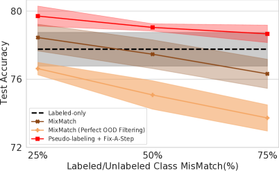
Figure 2: Demo of benefits of Phase 1 (MixMatch using all unlabeled images, even OOD) and Phase 2 (step direction), on CIFAR-10 6-animal task (400 examples/class). Results average across 5 train/test splits (shaded area shows standard deviation).

Fix-A-Step combines augmentation (phase 1) with protection against accuracy deterioration from the unlabeled loss (phase 2, described below) to “repair” SSL base models. A final takeaway from Fig. 2 is that Fix-A-Step can repair a nine-year-old method, Lee (2013)’s Pseudo-label, to beat MixMatch across all mismatch levels. While we tune hyperparameters for MixMatch here (see App. E), to compare fairly we do not tune hyperparameters for Fix-A-Step.

Algorithm 1 Fix-A-Step Training

Input: Labeled set $\mathcal{D}^{L}$, Unlabeled set $\mathcal{D}^{U}$ (uncurated)
Output: Trained weights $w$
Procedure

1:  for iter $i\in 1,2,\ldots I$ until converged do

2:     $\mathbf{x}^{L},\mathbf{y}^{L},\mathbf{x}^{U}\leftarrow{\textsc{GetNextMinibatch}}(\mathcal{D}^{L},\mathcal{D}^{U})$

3:     $\tilde{\mathbf{x}}_{1}^{U},\tilde{\mathbf{x}}_{2}^{U},\tilde{\mathbf{y}}^{U}\leftarrow{\textsc{Aug+PseudoLabel}}(\mathbf{x}^{U};w,\tau)$

4:     $\tilde{\mathbf{x}}^{L},\tilde{\mathbf{y}}^{L}\leftarrow{\textsc{MixMatchAug}}(\mathbf{x}^{L},\mathbf{y}^{L},\tilde{\mathbf{x}}_{1}^{U},\tilde{\mathbf{x}}_{2}^{U},\tilde{\mathbf{y}}^{U};\alpha)$

5:     $g^{L}\leftarrow\nabla_{w}\ell^{L}(\tilde{\mathbf{x}}^{L},\tilde{\mathbf{y}}^{L};w)$

6:     $g^{U}\leftarrow\nabla_{w}\ell^{U}(\tilde{\mathbf{x}}_{1}^{U},\tilde{\mathbf{y}}^{U};w)$

7:     $w\leftarrow\begin{cases}w-\epsilon(g^{L}+\lambda_{i}g^{U})~{}~{}&\text{if~{}}\sum_{d}g^{L}_{d}g^{U}_{d}>0\\ w-\epsilon g^{L}~{}&\text{o.w.}\end{cases}$

8:  end for

9:  return w

Hyperparameters (Values marked $\dagger$ tuned for all baselines as in App. E. No tuning for Fix-A-Step in any experiment.)

• Temperature $\tau{=}0.5$ for Aug+PseudoLabel (Alg. C.1)

• Beta dist. shape $\alpha{=}0.5$ for MixMatchAug (Alg. C.2)

• Step size $\epsilon$^†, Initial weights $w$, Max iterations $I$

• Unlabeled-loss weight per iter $\lambda_{1},\ldots\lambda_{I}$^†

Phase 2: Step direction modification. We address the possible harm from the unlabeled loss in phase 2 (lines 5-7 of Alg. 1), by modifying how neural net weights are updated. The idea is to only use gradient information from the unlabeled loss if it improves labeled-set performance.

At each batch, we compute two gradient vectors, one for each term in the loss: Let $g^{L}=\nabla_{w}\ell^{L}$ and let $g^{U}=\nabla_{w}\ell^{U}$. Our Fix-A-Step update for weights $w$ using step size $\epsilon$ is

$$w\leftarrow\begin{cases}w-\epsilon(g^{L}+\lambda g^{U})\!\!\!&\text{if~{}}\sum_{d}g^{L}_{d}g^{U}_{d}>0\\ w-\epsilon g^{L}&\text{otherwise}.\end{cases}$$ (2)

In the top case, we do the standard steepest descent update that minimizes the two-term SSL objective in Eq. (1). In the bottom case, we perform an alternative update, using only the labeled-term gradient. This two-case construction tries to ensure that SSL learning does not harm labeled set performance by “turning off” the gradient from an unlabeled batch when it interferes with the labeled loss. We give geometric intuition below, then formally show that the gradient update in Eq. (2) always move weights $w$ in a descent direction for the labeled set loss at the current minibatch.

Geometric intuition for Phase 2. Recall that two vectors $g^{L}$ and $g^{U}$ have positive inner product (top case update) only if the angle between the vectors is below 90 degrees, meaning their directions are similar. At angles larger than 90 (bottom case), $g^{L}$ and $g^{U}$ are pointing in different directions, and minimizing the unlabeled loss would hinder the labeled loss. In SSL, we care most about (heldout) classifier accuracy. Any improvement on the unlabeled loss is useful only if it helps improve accuracy. When $g^{U}$ points in a different direction than $g^{L}$, our update ignores the unlabeled gradient and updates weights $w$ using only $g^{L}$.

Definition 1: Descent direction of loss $\ell$. For any loss function $\ell$ for weight parameter vector $w\in\mathbb{R}^{D}$, a vector $v\in\mathbb{R}^{D}$ is a descent direction of $\ell$ at $w$ if the inner product satisfies $v^{T}\nabla_{w}\ell<0$ (Boyd and Vandenberghe, 2004).

Lemma 1: The update in Eq. (2) steps in a descent direction of the labeled loss $\ell^{L}$ at the current minibatch. We prove for each case in Eq. (2). Top case: By assumption, $\lambda>0$ and the inner product $\sum_{d}g^{L}_{d}g^{U}_{d}$ is positive. This implies that $v{=}-(g^{L}+\lambda g^{U})$ is a descent direction:

$$v^{T}g^{L}=\underbrace{-\textstyle\sum_{d}(g^{L}_{d})^{2}}_{\text{always negative}}\quad-\lambda\underbrace{\textstyle\sum_{d}g^{L}_{d}g^{U}_{d}}_{\text{pos. by assumption}}<0.$$ (3)

Bottom: $-g^{L}$ is a descent direction for $\ell^{L}$ by definition.

While Lemma 1 provides a justification for our approach, we cannot guarantee the labeled loss will decrease after each step, for the same reasons that stochastic gradient descent (SGD) does not always decrease the loss after each update: First, a descent direction of a minibatch may not be a descent direction of the entire dataset. Second, step size matters; if $\epsilon>0$ is too large, the loss may increase. Nevertheless, with proper step size tuning, SGD has been wildly successful by following minibatch-specific descent directions. Thus far, we find Fix-A-Step also successful.

Inspiration from multi-task learning. Our step direction modification in Eq. (2) was developed independently but is similar to previous algorithms for multi-task learning with a “main” task and an “auxiliary” task (Du et al., 2020). Others have explored variations of this “gradient surgery” (Yu et al., 2020b). To our knowledge, such ideas have not yet been suggested or validated for closed-set or open-set SSL.

Inspiration from continual learning. Our step modification phase is also inspired by the Transfer-Interference trade-off (Riemer et al., 2018; Lopez-Paz and Ranzato, 2017). This trade-off measures whether learning from one example will improve or impair learning on another example. These works formally define transfer as the case where the inner product of each example’s loss gradient with respect to weights is positive, and interference as the case where the inner product is negative. Other continual learning work also pursues this direction (Chaudhry et al., 2018; He and Jaeger, 2018; Zeng et al., 2019; Farajtabar et al., 2020). We extend this transfer-interference idea to SSL.

Simplicity compared to related work. We emphasize a key advantage of Fix-A-Step is extreme simplicity. Beyond the modest cost of MixMatch-like augmentation, we compute exactly the same losses and gradients as any standard deep SSL solving Eq. (1). Each possible weight update is straightforward. Determining which update to use depends only on an inner product, adding negligible runtime cost. Table 1 suggests Fix-A-Step is favorable to other open-set SSL approaches in its simplicity. There is no added complexity from extra backward passes, no extra neural networks that must be trained for OOD discrimination, no need for curriculum learning, and no expensive bi-level optimization problem to solve. Simplicity leads to faster training (App. A.5,  B.1) and (hopefully) easier adoption.

Synergy between Phase 1 and 2. One might wonder if our step direction modification in Phase 2 leads to overfitting the labeled loss. We argue that Phase 1’s augmentation should protect against overfitting, and our experiments thus far suggest overfitting is not a major concern.

4 EXPERIMENTS ON CIFAR

400 examples/class
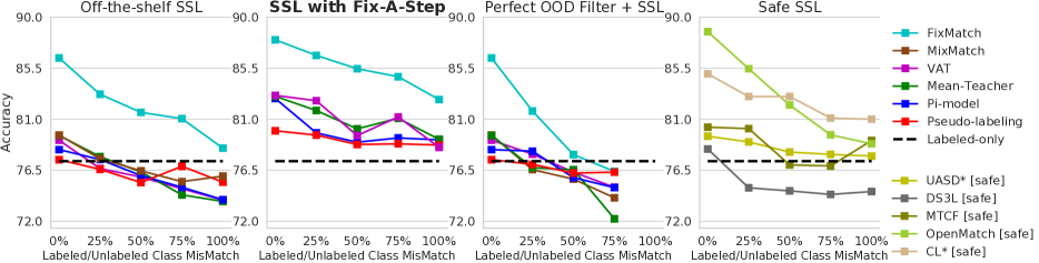
50 examples/class

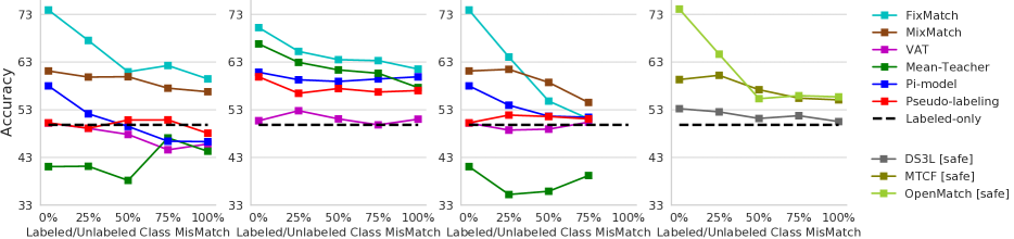
Figure 3: Accuracy on CIFAR-10 6 animal task. Accuracy on test images of animals (y-axis) as unlabeled set mismatch (percentage of non-animal classes represented, x-axis) increases. Column 1 (from left): Previous SSL methods trained in standard fashion. Col. 2: SSL methods trained with our Fix-A-Step. Col. 3: SSL methods with perfect OOD filtering of the unlabeled set (removing all non-animal images before training). Col. 4: Previous methods designed for open-set or safe SSL. UASD and CL (marked $*$) taken from its publication, others from our experiments. Top row: 400 examples/class; Bottom: 50 examples/class.

Our open source code uses PyTorch (Paszke et al., 2019) and allows reproducing each experiment (see App. E). Following Oliver et al. (2018), for all methods we use the same Wide ResNet-28-2 (Zagoruyko and Komodakis, 2016), apply standard augmentation (random crops, flips) on the labeled set, and regularize via weight decay.

Hyperparameters. All baselines use well-tuned hyperparameters for CIFAR-10 suggested by previous work  (see App. E). If a baseline underperformed, we retuned to maximize validation set accuracy. To be sure our reported gains are meaningful, we did no hyperparameter tuning at all for Fix-A-Step, fixing $\alpha=0.5,\tau=0.5$ throughout and inheriting other hyperparameters from the base SSL method.

SSL baselines. We compared to 6 closed-set SSL methods (Pi-Model, Mean-Teacher, Pseudo-label, VAT, MixMatch, and FixMatch) as well as the baseline that minimizes labeled loss $\ell^{L}$ on the labeled set (“labeled-only”). We also compare to 5 state-of-the-art methods intended for open-set/safe SSL: UASD (Chen et al., 2020d), DS3L (Guo et al., 2020), MTCF (Yu et al., 2020a), OpenMatch (Saito et al., 2021) and Curriculum-labeling (Cascante-Bonilla et al., 2021). If possible, we use our own implementations of baselines, ensuring architectures, training, and hyperparameters are comparable and reproducible. If a result is copied from another paper, we mark with an asterisk ($*$).

Training. Following choices in original implementations, each method is trained using either Adam with fixed learning rate or SGD with a cosine-annealing schedule for learning rate (Sohn et al., 2020). We found cosine-annealing and a slow linear ramp-up schedule for the unlabeled-loss-weight $\lambda$ particularly helpful for several baselines (see App. E). Each training run used one NVIDIA A100 GPU.

4.1 CIFAR-10 Protocol and Results

6-animal task for CIFAR-10. We pursue the “6-animal” task designed by Oliver et al. (2018) to artificially create unlabeled sets at different levels of mismatch with the labeled set. We build a labeled set of the 6 animal classes (dog, cat, horse, frog, deer, bird) in CIFAR-10, across two training set sizes: 50 labeled images per class and 400 per class. We form an unlabeled set of ${\sim}4100$ images/class from 4 selected classes, some animal and some non-animal (car, truck, ship, airplane). The percentage of non-animal classes is denoted by $\zeta$. If $\zeta=0\%$, we recover the standard “closed-set” SSL setting. At $\zeta=100\%$, the unlabeled set has no classes in common, and the OOD-filtering paradigm suggests that we should ignore the unlabeled set entirely. For details on the unlabeled set construction, see App. A.1.

Results on 6-animal. In Fig. 3, we compare the accuracy of different methods at recognizing the 6 animal classes in the test set, as the mismatch percentage $\zeta$ increases. Across two different training set sizes (rows), we compare 4 different training scenarios (columns, best read left to right): methods trained in the standard way (“off-the-shelf”), methods trained using Fix-A-Step, methods trained in the standard fashion but with perfect OOD filtering applied to the unlabeled set before training so that only known-class samples remain, and methods intended for safe SSL. The perfect OOD filtering column essentially shows the best-possible case for methods under the OOD-is-harmful paradigm.

We highlight several findings from Fig. 3:

1. Fix-A-Step improves all SSL methods in almost all settings. Despite its relative simplicity, Fix-A-Step is quite effective, as seen in the raised accuracies from the first to the second column across almost all methods and $\zeta$ values. Fix-A-Step with FixMatch base outperforms all other safe SSL methods (4th col.) for all mismatch levels $\zeta>0\%$. In Fig. A.3, we further demonstrate that Fix-A-Step’s gains are robust across multiple random train/test splits.

2. Perfect OOD filtering is not enough. The third column shows that perfect OOD filtering delivers underwhelming accuracy compared to Fix-A-Step for all $\zeta>0$. Our method’s gains over perfect filtering suggest that trying to benefit from OOD samples is more useful than filtering them. We suggest several explanations for the poor performance of perfect filtering, such as class imbalance even among known classes in the unlabeled set (Kim et al., 2020; Lai et al., 2022), sensitivity to hyperparameters (Su et al., 2021; Sohn et al., 2020), or perhaps how unlabeled data may affect the training via batchnorm  (Zhao et al., 2020). More work is needed to understand this phenomenon.

3. Fix-A-Step is faster than alternatives. For example, in the 400 examples/class $\zeta=50\%$ setting, using Fix-A-Step with a Mean-Teacher base delivers similar accuracy to OpenMatch (81.08 vs 79.62) while requiring less than half the training time (22 vs. 47 hr., App  A.5).

4.2 CIFAR-100 Protocol and Results

50-class task for CIFAR-100. Using the larger CIFAR-100 dataset, we follow the open-set SSL experimental design of Chen et al. (2020d) to create a $\zeta=50\%$ class distribution mismatch scenario by using classes 1-50 as labeled classes, and classes 25-75 as unlabeled classes. To assess a more extreme level of unlabeled set “contamination”, we further create a 100% class distribution mismatch scenario: classes 1-50 are labeled classes; classes 51-100 unlabeled.

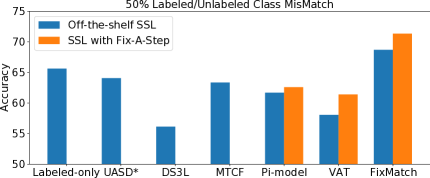
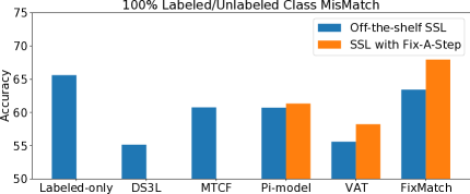
Figure 4: Accuracy on CIFAR-100 50-class task. Each bar represents the accuracy of a method with either off-the-shelf training (blue) or Fix-A-Step (orange). We try 2 scenarios: 50% labeled/unlabeled class mismatch (left panel) and 100% class mismatch (right). All numbers were produced by our implementation except those marked $*$ (UASD).

Results on CIFAR-100 50-class. Fig. 4 compares “off-the-shelf” SSL methods using standard training (blue bars) and Fix-A-Step (orange). We see consistent gains at both 50% and 100% mismatch, even without tuning hyperparameters.

4.3 Ablations and Sensitivity Analysis

Ablations. We quantify how each of Fix-A-Step’s two key components (Augmentation and Gradient step modification) perform in isolation. Tab. 2 compares accuracy on the 6 animal task at 400 examples/class and $\zeta=100\%$. Gradient step modification alone increases accuracy around 0.5 to 1.5% across five base SSL methods. Augmentation alone increases accuracy around 2.5 to 4.5%. When combined, we consistently see the largest gains. Although we didn’t tune hyperparameters, we expect enlarging batch size may lead to more gain from gradient step modification, since it gives less noisy estimates of the gradient alignment. For further results at other mismatch levels, see App. A.

Sensitivity analysis. There are two hyperparameters unique to Fix-A-Step: sharpening temperature $\tau{>}0$ and the Beta shape $\alpha{>}0$. For simplicity, we set $\alpha{=}0.5$ and $\tau{=}0.5$ throughout. Since deep SSL is often sensitive to hyperparameters, we further analyse other possible choices: $\alpha{\in}\{0.5,0.75\}$ and $\tau{\in}\{0.5,0.95\}$. Fig. A.4 shows that Fix-A-Step delivers consistent and similar accuracy gains across all tested $\alpha,\tau$ settings, and thus does not appear overly sensitive.

	Pi-Model	MT	VAT	Pseudo	FixMatch
off-the-shelf	73.90	73.75	73.87	75.45	78.45
+G only	74.50	74.33	75.35	75.92	79.73
+A only	77.25	78.38	77.87	77.88	81.53
+A&G (ours)	79.18	79.23	78.52	78.72	82.73

Table 2: Ablations for CIFAR-10 6 animal task, reporting accuracy for each SSL method (columns) if we only use our augmentation (+A), only use our gradient step modification (+G), or use the combination (+A&G) that defines Fix-A-Step. We bold the best result and all others within 1 percentage point. Setting: 400 examples/class, $\zeta=100\%$.

5 EXPERIMENTS ON HEART2HEART

TMED2 (Boston, USA; 4 views)	Transfer to Unity (UK; 3 views)	Transfer to CAMUS (France, 2 views)

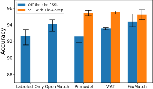
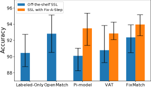
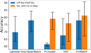
Figure 5: Balanced accuracy for echocardiogram view classification (Heart2Heart benchmark). Methods are trained on TMED-2 images to distinguish 4 view types: PLAX, PSAX, A2C, and A4C. TMED2’s 353,500 image unlabeled set is uncurated, representing a superset of possible view types including the 4 known classes. Bar height gives mean balanced accuracy across 3 models trained on different splits of TMED-2 (error bars indicate min/max). Left: Evaluation on heldout TMED-2 images. Center: Evaluation of TMED-2-trained classifiers on PLAX, A2C, and A4C images from Unity dataset (17 sites in the UK). Right: Evaluation of TMED-2-trained classifiers on A2C and A4C views from CAMUS dataset (1 site in France).

In pursuit of realistic evaluation, we consider a reproducible, clinically-relevant SSL task that we call Heart2Heart. The key question is this: can we transfer classifiers trained on ultrasound images of the heart from one hospital system to new heart images from unrelated hospitals in other countries. For training, we use the Tufts Medical Echocardiogram Dataset 2 (TMED-2) (Huang et al., 2022a, 2021b), collected in Boston, USA. TMED-2 has a small labeled set of echocardiogram studies and a larger uncurated unlabeled set. Thanks to common device standards, these images are interoperable with two other datasets of “echo” images: Unity from 17 hospitals in the UK (Howard et al., 2021) and CAMUS from a hospital in France (Leclerc et al., 2019). We emphasize that all datasets are deidentified and accessible to any academic researcher.

Classification task: View type of 2D TTE image. Trans-thoracic echocardiography (TTE) is a gold-standard way to non-invasively capture the heart’s 3-dimensional anatomy for measurement and diagnosis. A human sonographer wields a handheld transducer over the patient’s chest at different angles in order to provide clear views of each facet of the heart. A routine TTE scan of a patient, called a study, produces many images (median=68, 10-90th percentile range=27-97 in TMED-2), each showing a canonical 2D view of the heart. No view type annotation is recorded with any image. In later analysis, clinicians manually search over all images to find a desired view type. Automated interpretation of echocardiograms must also be able to pick out specific view types before any useful measurements or diagnosis can be made, making view classification a prediction task with potential clinical impact (Madani et al., 2018a; Huang et al., 2021b).

TMED-2 provides set of labeled images of four specific view types, known as PLAX, PSAX, A2C, and A4C, gathered from certified annotators. Reliably identifying these views would be particularly useful for key valve disease diagnostic tasks (Huang et al., 2021b; Wessler et al., 2023). TMED-2 also contains a truly uncurated unlabeled set of 353,500 images from routine TTEs from 5486 patient-studies. At least 9 canonical view types frequently appear in routine TTEs (Mitchell et al., 2019), so this unlabeled set should contain extra classes not in the labeled set. However, this view classification problem on TMED-2 is more than just “open-set” SSL, because TMED-2 labeled and unlabeled sets were not identically sampled from the same patient population, which leads to some modest feature differences. Unlabeled echos come from all available files for convenience, while the the labeled set deliberately oversamples patients with a valve disease called aortic stenosis (AS). About 50% of all patients in the labeled set have severe AS, compared to less than 10% in the general population. For severe AS patients, PLAX and PSAX images will show heavier calcification (thickening) of the aortic valve.

Protocol. Averaging over TMED-2’s recommended 3 splits, we train each SSL method on images from 56 labeled studies as well as all unlabeled studies (353,500 images). We report balanced accuracy on each split’s test set of 120 studies ($\sim$2104 images). We then assess generalization of these Boston-based classifiers to images from European hospitals. We report balanced accuracy on 7231 available PLAX, A2C, and A4C images from Unity, as well as all 2000 images (A2C and A4C views) in CAMUS.

Results on Heart2Heart. Fig. 5 shows classifier performance on held-out data from all 3 datasets. TMED-2 evaluations (first panel) show that our Fix-A-Step procedure yields gains across all tested SSL methods (Pi-Model, VAT, FixMatch). Fix-A-Step helps all three methods convincingly outperform the labeled-only baseline. Compared to OpenMatch, a state-of-the-art safe SSL method, Fix-A-Step yields better accuracy while being much simpler. We also find that Fix-A-Step delivers competitive accuracy considerably faster ($\sim$2-3x speedup, See App.  B.1).

External evaluation on Unity and CAMUS (Fig. 5 panels 2-3) show that these gains transfer to new hospitals. Each tested SSL method performs better with Fix-A-Step than standard training. Across splits we see larger performance variation on Unity and CAMUS than on TMED-2, which highlights the difficulty of generalizing across hospitals as well as importance of external validation. All methods perform worse on CAMUS than other datasets; see App. B for further investigations. Overall, this Heart2Heart benchmark task shows the promise of Fix-A-Step to deliver gains from unlabeled data that generalize better than alternatives.

6 DISCUSSION

In summary, this paper makes three contributions to deep SSL image classification. First, we argue that uncurated or OOD data in the unlabeled set can be helpful, and should not merely be filtered out. Experiments in Fig. 3 show that even with perfect OOD filtering most SSL methods deliver underwhelming accuracy gains. Second, we introduce a new training procedure called Fix-A-Step that achieves state-of-the-art SSL performance on uncurated unlabeled sets while being faster and simpler (no new loss terms or extra neural nets). Finally, we hope our new Heart2Heart benchmark for SSL evaluation inspires robust studies of clinical model transportability across global populations.

Limitations. Our work’s exclusive focus is image classification. More work is needed to try Fix-A-Step on other data types like time series. Our experiments on artificial unlabeled sets in Sec. 4 focused exclusively on mismatch in the labels. We did not systematically explore how shifts in the features $x$ between the labeled and unlabeled set impact performance, though we do emphasize that TMED-2’s uncurated unlabeled set likely has such shifts due different acquisition criteria (see Sec. 5). Fix-A-Step’s phase 2 step modification does not guarantee accuracy gains, only protects against possible deterioration. Omitting unlabeled loss gradients because of harm to a minibatch labeled loss may miss a chance to improve accuracy globally. Recently, Schmutz et al. (2022) found that the optimal choice of the unlabeled loss coefficient $\lambda$ depends on the covariance matrix between $g^{L}$ and $g^{U}$, which might provide another way to consider the step modification phase.

Impact statement. Work on SSL is often motivated by its promise in medical imaging (Huang et al., 2021b; Madani et al., 2018b). Our Heart2Heart evaluation shows a proof-of-concept for generalization of ultrasound view classifiers across hospitals. More work is needed to rigorously assess generalizability and translate to improved patient care. Extra effort is needed to avoid widening current disparities (Celi et al., 2022), as the data sources in our Heart2Heart benchmark do not reflect the geographic and racial diversity of many patient populations.

Outlook. Fix-A-Step is a promising new first-line approach to SSL that can unlock the promise of uncurated unlabeled sets. We hope future work explores augmentation and step direction further, while extending our focus on simplicity, reproducibility, and possible benefits of OOD images.

Acknowledgements

We acknowledge financial support from the Pilot Studies Program at the Tufts Clinical and Translational Science Institute (Tufts CTSI NIH CTSA UL1TR002544) and computing infrastructure support from NSF OAC CC* 2018149. Author B. W. was supported in part by K23AG055667 (NIH-NIA). Author M.-J. S. was supported by the Tufts Summer Scholars Program.

Supplementary Material

In this supplement, we provide:

• Sec. A: CIFAR Experiments: Further Details, Results, and Analysis

• Sec. B: Heart2Heart Experiments: Further Details, Results, and Analysis

• Sec. C: Methods Supplement: Algorithms for Aug+SoftLabel and MixMatchAug

• Sec. D: Related Work Supplement: Further Discussion and Analysis

• Sec. E: Reproducibility Supplement: Hyperparameters, Settings, etc.

Appendix A CIFAR EXPERIMENTS: Details, Results, and Analysis

A.1 CIFAR-10 6-animal task mismatch description

In Table A.1 we define which classes form the labeled and unlabeled set at each level of mismatch for the CIFAR-10 6 animal task. This exactly follows  Oliver et al. [2018] and creates more challenging scenarios than other “mismatch” tasks on CIFAR-10 tried previously (for example,  [Saito et al., 2021] examine a case with all 10 classes in the unlabeled set).

	Labeled set	Unlabeled set
$\zeta=0\%$	Bird, Cat, Deer, Dog, Frog, Horse	Deer, Dog, Frog, Horse
$\zeta=25\%$	Bird, Cat, Deer, Dog, Frog, Horse	Airplane, Dog, Frog, Horse
$\zeta=50\%$	Bird, Cat, Deer, Dog, Frog, Horse	Airplane, Car, Frog, Horse
$\zeta=75\%$	Bird, Cat, Deer, Dog, Frog, Horse	Airplane, Car, Ship, Horse
$\zeta=100\%$	Bird, Cat, Deer, Dog, Frog, Horse	Airplane, Car, Ship, Truck

Table A.1: Definition of labeled/unlabeled class mismatch scenario in CIFAR-10 6 animal task. We bolded the non-animal classes in unlabeled set that are not in the labeled set. All included classes are represented with equal frequency.

A.2 Ablation Study across different level of contamination

Expanding on the ablation table in the main paper, in Tab. A.2 we show ablation comparisons (augmentation only, gradient step modification only, or both) across all tested values of the mismatch in labeled-vs-unlabeled class content $\zeta$.

Mismatch $\zeta=0\%$	Mismatch $\zeta=25\%$
+A only +G only +A&G (Fix-A-Step) Pi-Model 78.32 81.90 78.48 82.83 Mean-Teacher 79.57 84.18 80.60 83.02 VAT 79.15 83.88 79.47 83.10 Pseudo-label 77.43 79.03 78.30 79.98 FixMatch 86.40 86.35 86.17 88.00	+A only +G only +A&G (Fix-A-Step) Pi-Model 77.45 79.12 78.00 79.80 Mean-Teacher 77.70 81.35 78.28 87.77 VAT 76.65 82.27 78.35 82.63 Pseudo-label 76.58 79.28 77.25 79.60 FixMatch 83.20 84.44 83.85 86.63
Mismatch $\zeta=50\%$	Mismatch $\zeta=75\%$
+A only +G only +A&G (Fix-A-Step) Pi-Model 76.03 78.70 76.57 78.97 Mean-Teacher 76.35 82.22 78.18 80.15 VAT 75.90 79.43 77.37 79.56 Pseudo-label 75.42 78.33 75.65 78.77 FixMatch 81.60 83.28 81.80 85.45	+A only +G only +A&G (Fix-A-Step) Pi-Model 75.00 77.82 74.77 79.35 Mean-Teacher 74.33 79.63 74.52 81.08 VAT 74.87 80.82 75.20 81.20 Pseudo-label 76.85 78.38 77.15 78.83 FixMatch 81.05 83.03 81.33 84.75

Table A.2: Ablation analysis on CIFAR-10 6 animal task, examining how accuracy changes for each SSL method if we only use our augmentation (+A), only use our gradient step modification (+G), and use the combination (+A&G) which constitutes our Fix-A-Step. Each panel shows results for a fixed value of the mismatch percentage $\zeta$ describing the overlap in classes between labeled and unlabeled set. For each method, we bold the best result. Setting: 400 examples/class.

A.3 Robustness of results across multiple train/test splits

In the main paper, we report results on CIFAR-10 6 animal task across many baselines methods. For each baseline, we use only one train/test split due to the huge computation required to compare all baselines. In Fig. A.3, for a subset of methods we assess the robustness of the conclusions of that experiment across multiple separate training/test splits.

We train the labeled-set-only baseline, FixMatch with and without Fix-A-Step, and Mean-Teacher with and without Fix-A-Step for 5 random splits of the data, across two levels of mismatch ($\zeta=50\%$ and $\zeta=100\%$). Results are in Fig. A.3. Broadly, we suggest that our conclusion that Fix-A-Step delivers successful accuracy gains holds even across 5 splits: both FixMatch and MeanTeacher show notable gains across both levels of mismatch $\zeta$. Notably, MeanTeacher plus Fix-A-Step appears quite competitive with off-the-shelf FixMatch, and FixMatch plus Fix-A-Step is the best of all.

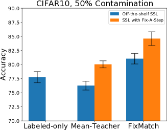
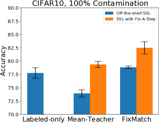
Figure A.3: CIFAR10, 400 examples/class. Bar height indicates the average across 5 random splits of the data. Error bars show the standard deviation across 5 splits.

A.4 Sensitivity to hyperparameters

Since Deep SSL methods could be sensitive to hyper-parameters, we conduct sensitivity analysis to see how Fix-A-Step behave under different choice of sharpening temperature $\tau$ and Beta distribution shape $\alpha$. We analyzed the performance of Fix-A-Step using a Mean-Teacher base model across several reasonable choices of MixUp parameter $\alpha{\in}\{0.5,0.75\}$ and sharpening temperature $\tau{\in}\{0.5,0.95\}$ (totally 4 combinations). (See. Alg. 1 for hyperparameter definitions). Results in Fig. A.4 shows that Fix-A-Step’s performance gains over the off-the-shelf (or “vanilla”) Mean Teacher base do not appear overly sensitive to these hyperparameters.

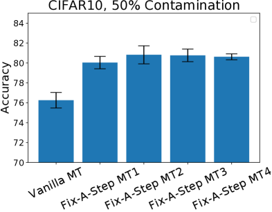
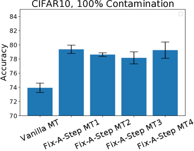
Figure A.4: CIFAR10, 400 examples/class. Vanilla MT: Mean teacher SSL base model. Fix-A-Step MT1: MT base Fix-A-Step with $\tau=0.5$ , $\alpha=0.5$, . Fix-A-Step MT2: MT base Fix-A-Step with $\tau=0.95$, $\alpha=0.75$. Fix-A-Step MT3: MT base Fix-A-Step with $\tau=0.5$, $\alpha=0.75$. Fix-A-Step MT4: MT base Fix-A-Step with $\tau=0.95$, $\alpha=0.5$. Results average across 5 random split of the data. Error bar showing standard deviation across the 5 split.

A.5 Comparison of computation cost and performance

Methods	$\zeta=25\%$		$\zeta=50\%$		$\zeta=75\%$
	Acc	Runtime	Acc	Runtime	Acc	Runtime
MT+Fix-A-Step	81.77	1476	80.15	1331	81.08	1333
VAT+Fix-A-Step	82.63	1662	79.56	1691	81.20	1681
OpenMatch	85.45	2728	79.56	2803	79.62	3270

Table A.5: Comparison of runtime and test accuracy on CIFAR-10 6 animal task. Setting: 400 example/class. Mismatch percentage $\zeta$ describes the overlap in classes between labeled and unlabeled set. Runtime (in minutes) is based on training same number of steps on a Nvidia A100 GPU.

Appendix B HEART2HEART EXPERIMENTS: Details, Results, and Analysis

B.1 Comparison of computation cost and performance

Methods	split0		split1		split2
	Acc	Runtime	Acc	Runtime	Acc	Runtime
Pi-model+Fix-A-Step	95.33	233	95.08	240	95.73	218
VAT+Fix-A-Step	95.58	392	95.30	343	95.66	356
OpenMatch	94.54	1244	94.59	1282	93.22	879

Table B.1: Comparison of runtime and test balanced accuracy on TMED-2 view classification task. Runtime in minutes. Each model is trained on a Nvidia A100. In practice, we found OpenMatch converges slower than alternatives compared, we thus train about 2x more iterations for OpenMatch (otherwise its accuracy performance would be worse).

B.2 Preprocessing TMED-2 data

We applied for access to the TMED-2 data via the form on the website (https://TMED.cs.tufts.edu), and downloaded the shared folder of data from the provided cloud-based link after approval. Images (as 112x112 PNG images) and associated view labels (in CSV files) are readily available in the provided shared folder for download.

Train/validation/test splits. To form our labeled sets for training, we used the provided train/test splits of the fully-labeled set with the smallest training set size (56 studies available for both training and validation). While larger labeled training sets are possible, we selected this smaller size as the most compelling use case for SSL. We wanted to answer the question: how well can we do with very little labeled data but a large pile of unlabeled data.

View label selection. Among available view labels, we chose PLAX, PSAX, A4C, and A2C as the 4 classes to focus on for our Heart2Heart view type classifier. The original TMED-2 labeled set, as described in Huang et al. [2022a], contains an additional view type label that they called A2CorA4CorOther, which is a super-category that contains possible view types distinct from PLAX and PSAX (including A2C, A4C, and other possible classes like A5C). For simplicity, we excluded that class in our Heart2Heart experiments.

B.3 Preprocessing Unity data

We downloaded the Unity data by going to their website (https://data.unityimaging.net). Once at their website, go to the ’Latest Data Release’ section and download the images. For the view labels, go to https://data.unityimaging.net/additional.html and download the csv file under the ’View’ section.

In the Unity dataset, along with PLAX, A2C, and A4C views, there are also A3C and A5C. For the purposes of these experiments, we filtered out all A3C and A5C images.

Disclaimer: These view labels were done by one human so there may be some errors in the labeling.

The raw Unity data came in .png format, so first we converted all the pngs to a tiff format. Then we converted them to gray-scale, padded the shorter axis to achieve a square aspect ratio, and resized it to 112 x 112 pixels.

B.4 Preprocessing CAMUS data

We acquired the CAMUS data by going to their website (http://camus.creatis.insa-lyon.fr/challenge/#challenges). Once you get to their website, link on the first link, register on that website, and then you’ll be free to download the dataset.

In the CAMUS dataset, in addition to having view labels (’2CH’ in their dataset is ’A2C’ and likewise ’4CH’ is ’A4C’), they also label whether the view was taken in the end diastolic (ED) or end systolic (ES) portion of the cardiac cycle. We separated and took note of these labels, but we found no significant differences in the results.

The raw CAMUS data came in .mhd format, a special file types used specifically for medical imaging. Through conversations with data creators, we discovered that the resolution for these images was lower in the x direction than the y direction and the way .mhd files compensate for a lower resolution is by adjusting the space between the pixels in that direction (indicated by the ’Element Spacing’ field). In order to convert to a standardized tiff file representation (where the spacing between pixels is uniform across width and height) we shrank the image in the y direction as:

$$y^{*}=\frac{y\cdot s_{y}}{s_{x}}$$ (4)

where y is the original location (number of pixels) in the y direction, $s_{y}$ and $s_{x}$ are the spacing of pixels in the y and x directions (as given in the Element Spacing metadata), and $y^{*}$ is the new location the y direction.

After this transformaion, the images were converted them to gray-scale, padded the shorter axis to achieve a square aspect ratio, and resized to 112 x 112 pixels.

B.5 Further investigation of CAMUS performance

In our main paper’s Fig. 5, we assess how well our TMED-2-trained models, which get balanced accuracy in the range $92-96\%$ on TMED-2 test set, generalize to other external datasets. The models did reasonably generalize to the Unity dataset (balanced accuracy ranges from $90-94\%$), however on the CAMUS dataset we saw all methods reach somewhat surprisingly lower overall performance (balanced accuracy $60-85\%$), though the relative ranking of different methods was similar.

Visualizing differences. To investigate, we visually compared images from TMED-2, Unity, and CAMUS. While Unity and TMED-2 looked similar, when comparing TMED-2 and CAMUS there are clear discrepancies in pixel intensity, likely from the use of a different ultrasound machine and different conventions standard intensity values and normalization. Fig.  B.2 below provides sample images of the two datasets and a summary histogram of pixel intensity (aggregated across all images).

Idea: Simple quantile transformation. To quickly try to remedy this discrepancy, we tried to transform the CAMUS images such that the pixel intensity distribution more closely resembles that of TMED-2. In this transformation, we first mapped all the target pixels to its empirical quantile (value between 0-1) and then we mapped that value to a pixel intensity in the source (TMED-2) images via the empirical inverse CDF. To see the effects of this transformation on the CAMUS images and on the pixel intensity histogram, look at the right-most panel of Fig. B.2

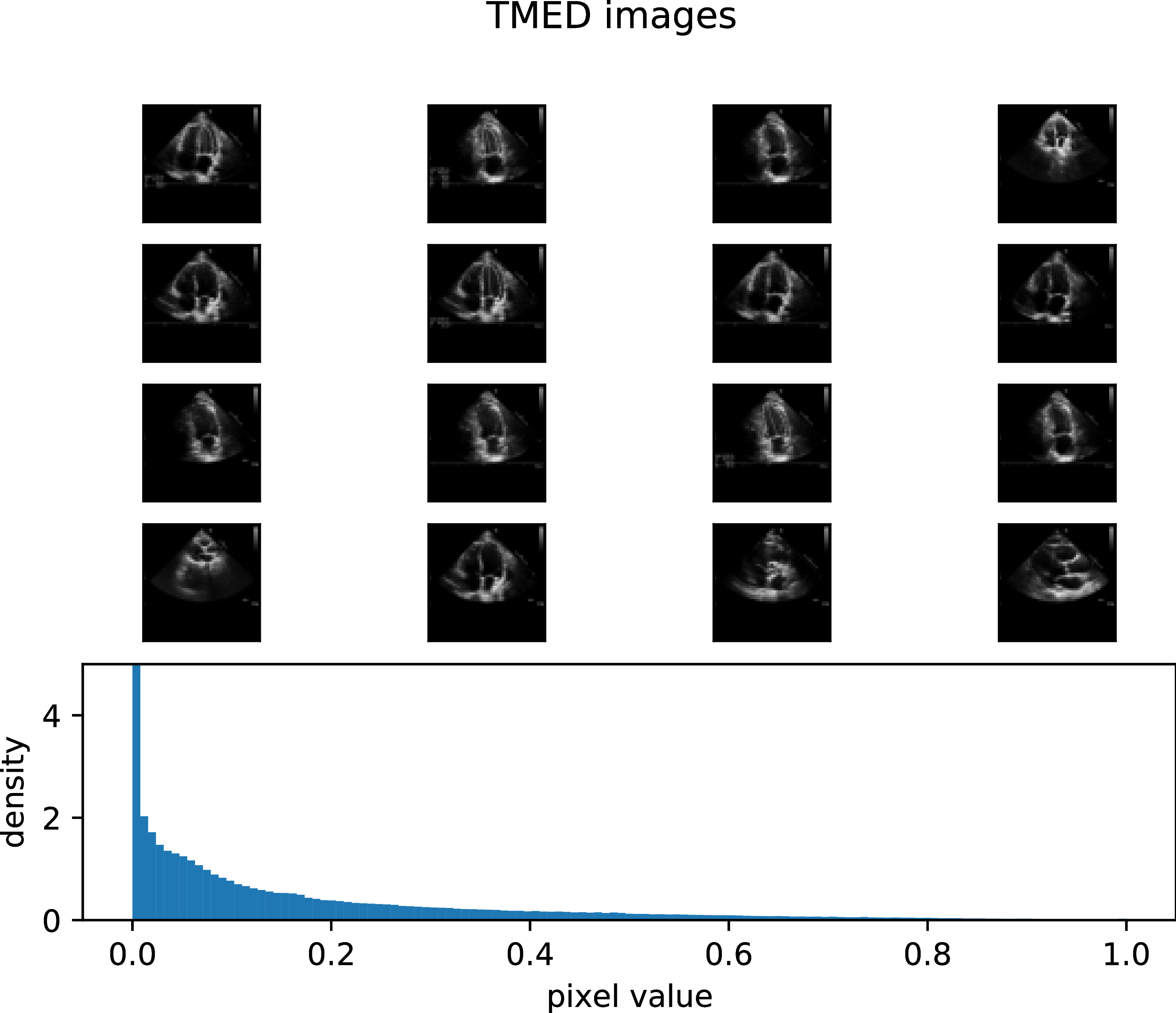
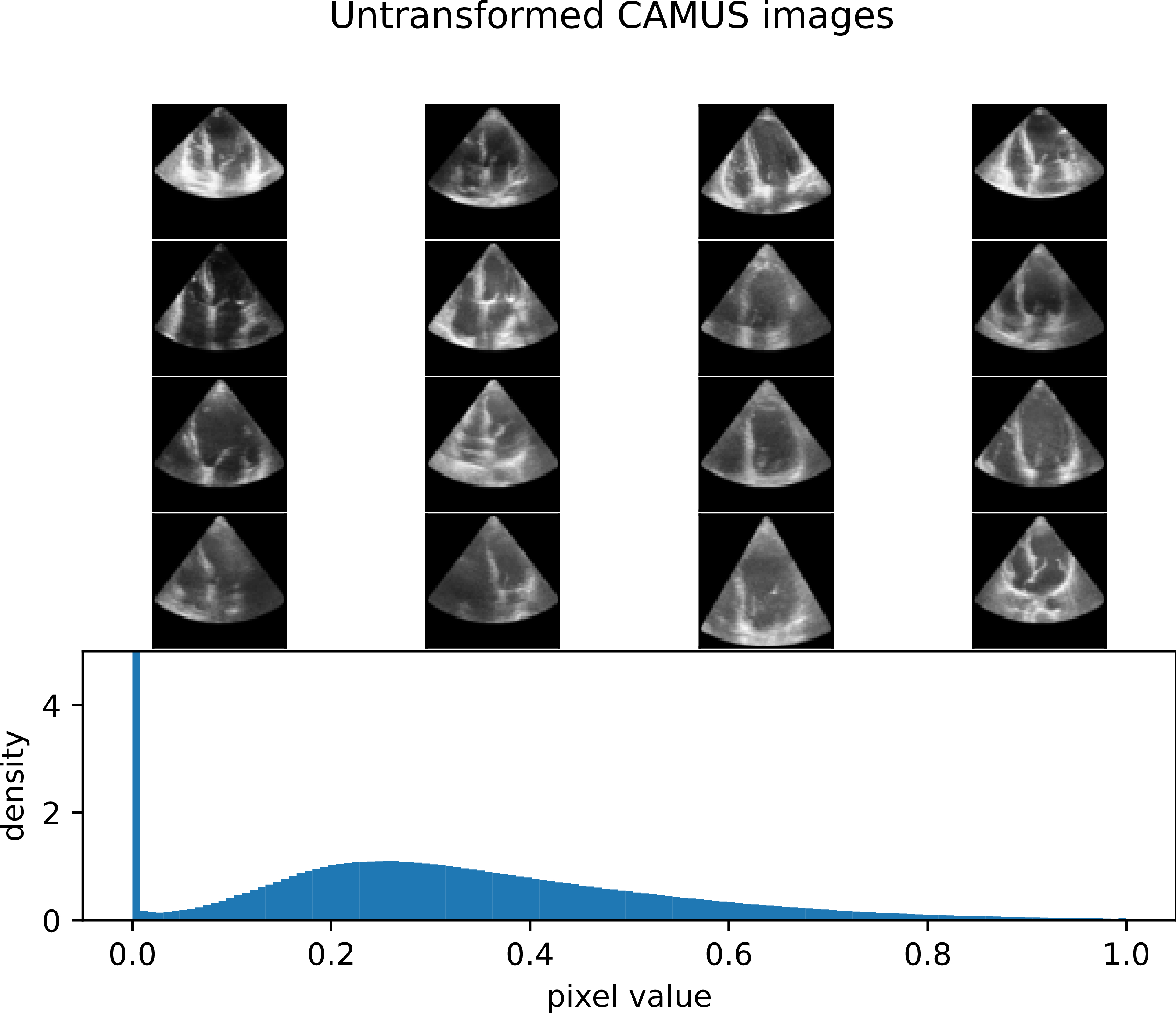
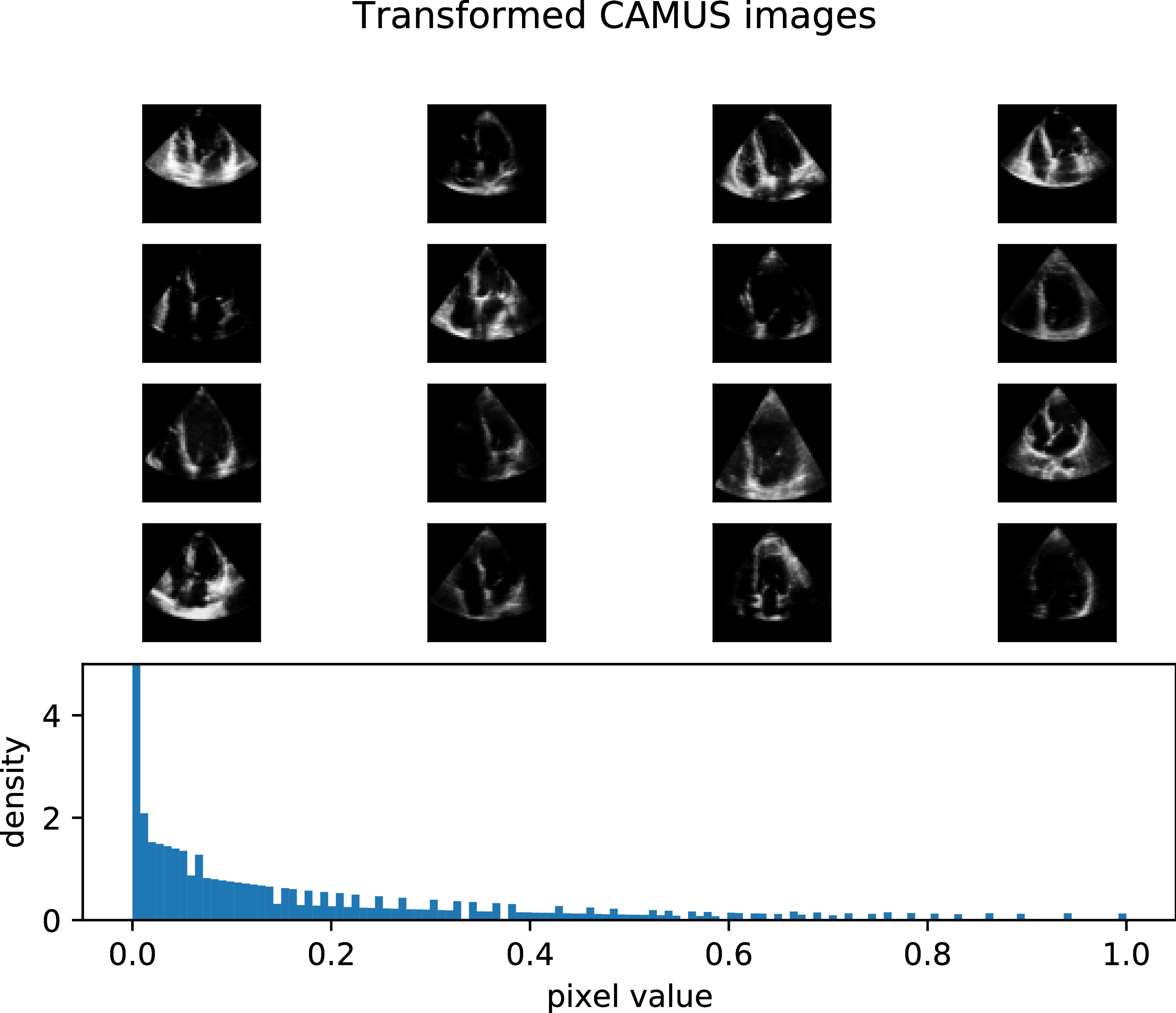
Figure B.2: A sample of images from the TMED-2 dataset, CAMUS dataset, and the same CAMUS pictures except under a pixel transformation to match the pixel intensity of TMED-2

Results after transform. The accuracy of the TMED-2-trained classifiers on both untransformed and transformed CAMUS data can be viewed in Fig. B.3. Like we said in the main paper, Fix-a-Step clearly improves SSL models in classifying CAMUS view types for the untransformed data. However, while the transformation itself seems to help model performance overall, Fix-a-Step doesn’t seem to help as much in the transformed dataset (some gains for VAT, but both FixMatch and Pi-model the before-after difference seems negigible). Importantly, Fix-A-Step is still competitive with its base method, just not notably superior to it. Much more work is needed here. In the future, we hope to explore other ways to improve performance on the CAMUS dataset so it reaches accuracy levels seen in the Unity dataset.

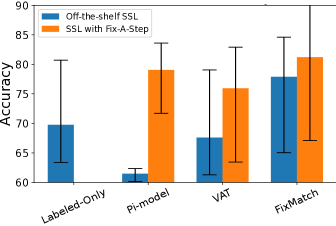
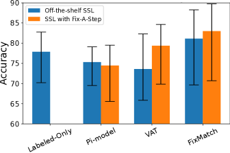
Figure B.3: Evaluation of the SSL methods from the paper on untransformed and transformed CAMUS images

Further investigation: Differences across splits. After investigating the results of the three data splits, we noticed that the first split seemed to significantly under perform on the CAMUS dataset, specifically with the A4C class. When we took a look at the Unity data for this split, we also noticed that, while the discrepancy wasn’t as drastic, the A4C class did under perform when compared to the other classes. These results can be clearly seen in Tab.  B.4. In all method-dataset pairs, A4C performs significantly worse than other classes.

A hypothesis we have is that this data split significantly under represents A4C and thus is not able to predict it as well. The reason why we don’t see TMED-2 and Unity significantly under perform in this split in terms of total balance accuracy is because the other classes are a significant portion of their test sets so they’re not as affected by A4C under performing; however, 50% of CAMUS is A4C, so that dataset is affected to a higher degree. However, we are unsure as to why the A4C class accuracy in CAMUS does significantly worse than the A4C class accuracy in Unity. We will investigate this discrepancy further in the future. We think this open problem makes our Heart2Heart benchmark especially interesting.

Methods	CAMUS		Unity
	A4C	A2C	A4C	A2C	PLAX
Labeled-Only	28.8	98.0	76.9	93.3	96.1
Pi-model	27.1	96.8	81.9	93.1	98.2
Pi-model w/ FAS	45.4	98.0	87.5	94.1	99.6
VAT	26.6	98.3	77.0	93.1	97.7
VAT w/ FAS	27.5	99.4	84.6	96.2	95.5
Fix-Match	34.1	96.0	79.8	94.8	96.9
Fix-Match w/FAS	36.3	97.9	83.5	95.2	99.0

Table B.4: Class accuracies for data split 1 across methods for the Unity dataset and untransformed CAMUS dataset. Bolded are the lowest class accuracies for each dataset-method pair.

Appendix C METHODS SUPPLEMENT

Here, we provide implementation details of the two subprocedures in our Fix-A-Step training (Alg. 1). Both procedures were originally proposed by MixMatch [Berthelot et al., 2019], we provide them here in common notation as the rest of our paper for clarity.

First, the algorithm Aug+SoftLabel is in Alg. C.1. This procedure consumes a batch of raw images from the unlabeled set and returns two transformed batches, with a common set of “sharpened” soft (probabilistic) labels.

Second, the algorithm MixMatchAug is in Alg. C.2. This procedure consumes a batch of raw labeled data, and produces a transformed batch of the same size.

Algorithm C.1 Augment and Soft-Pseudo-Label

Input: Unlabeled batch features $\mathbf{x}^{U}$
Output: Augmented features $\mathbf{x}^{U}_{1},\mathbf{x}^{U}_{2}$, Soft pseudo labels $\tilde{\mathbf{y}}^{U}$
Hyperparameters

• Sharpening temperature $\tau{>}0$

Procedure

1:  for each image $x$ in $\mathbf{x}^{U}$ do

2:     $x^{(1)}\leftarrow\text{BasicImageAugment}(x_{n})$

3:     $x^{(2)}\leftarrow\text{BasicImageAugment}(x_{n})$

4:     $\rho^{(1)}\leftarrow f_{w}(x^{(1)})$         // Probability vector predicted by neural net

5:     $\rho^{(2)}\leftarrow f_{w}(x^{(2)})$

6:     $\tilde{r}\leftarrow\left(\frac{1}{2}\rho^{(1)}+\frac{1}{2}\rho^{(2)}\right)^{1/\tau}$   // Non-negative vector, sharpened by element-wise power

7:     $S\leftarrow\sum_{c}\tilde{r}_{c}$

8:     $\tilde{y}\leftarrow[\frac{\tilde{r}_{1}}{S},\frac{\tilde{r}_{2}}{S},\ldots\frac{\tilde{r}_{C}}{S}]$       // Normalize to ‘‘soft’’ label (proba. vector)

9:     Add $x^{(1)}$ to $\tilde{\mathbf{x}}^{U}_{1}$

10:     Add $x^{(2)}$ to $\tilde{\mathbf{x}}^{U}_{2}$

11:     Add $\tilde{y}$ to $\tilde{\mathbf{y}}^{U}$

12:  end for

13:  return $\tilde{\mathbf{x}}^{U}_{1}$, $\tilde{\mathbf{x}}^{U}_{2}$, $\tilde{\mathbf{y}}^{U}$

Algorithm C.2 MixMatchAug : Transformation of Labeled Set

Input: Labeled batch $\mathbf{x}^{L},\mathbf{y}^{L}$, Unlabeled batch $\mathbf{x}^{U},\tilde{\mathbf{y}}$,
Output: Transformed labeled batch $\mathbf{\tilde{x}}^{L},\mathbf{\tilde{y}}^{L}$
Hyperparameters

• Shape $\alpha{>}0$ of $\text{Beta}(\alpha,\alpha)$ dist.

1:  for image-label pair $x,y$ in labeled batch ${\mathbf{x}^{L},\mathbf{y}^{L}}$ do

2:     $x^{\prime},y^{\prime}\leftarrow\textsc{SampleOnePair}([\mathbf{x}^{L},\tilde{\mathbf{x}}^{U}_{1},\tilde{\mathbf{x}}^{U}_{2}],[\mathbf{y}^{L},\tilde{\mathbf{y}}^{U},\tilde{\mathbf{y}}^{U}])$

3:     $\beta^{\prime}\sim\textsc{SampleFromBeta}(\alpha,\alpha)$

4:     $\beta\leftarrow\textsc{Max}(\beta^{\prime},1-\beta^{\prime})$

5:     $\tilde{x}\leftarrow\beta x+(1-\beta)x^{\prime}$

6:     $\tilde{y}\leftarrow\beta y+(1-\beta)y^{\prime}$

7:     Add $\tilde{x}$ to $\tilde{\mathbf{x}}^{L}$

8:     Add $\tilde{y}$ to $\tilde{\mathbf{y}}^{L}$

9:  end for

10:  return $\tilde{\mathbf{x}}^{L},\tilde{\mathbf{y}}^{L}$

Fix-A-Step with FixMatch. Here, we further clarify how Fix-A-Step works with FixMatch-base. In the original FixMatch, each unlabeled image generates one weakly augmented version and one strongly-augmented. With Fix-A-Step, an additional weakly augmented version is generated. The two weak images are used in the Fix-A-Step augmentation phase to transform the labeled set. The unlabeled loss is calculated using one weak and one strong image as in FixMatch. In this work, we used the original images for unlabeled loss calculation (not the transformed images from FixAStep augmentation phase) so that only the unlabeled set affect the labeled set but not vise versa, since we focus on analyzing the value of the unlabeled set to the labeled set. Network parameters are updated via Algorithm 1 line 5-7.

Appendix D RELATED WORK SUPPLEMENT

SSL benchmarks.

SSL methods continue to focus a few datasets intended for fully-supervised image classification, such as SVHN, CIFAR-10, CIFAR-100, and ImageNet. This is a problem because these data are post-hoc repurposed for SSL, dropping known labels to create unlabeled sets in artificial fashion. The resulting unlabeled sets are too curated: images usually come from the same classes as the labeled set with similar frequencies. However, real applications that motivate SSL require an easy-to-acquire unlabeled set that is uncurated.

Recent research has further identified problems with CIFAR and ImageNet. First, 3% of CIFAR-10 and 10% of CIFAR-100 test images have perceptually-indistinguishable duplicates in the train set [Barz and Denzler, 2020]. This questions whether high-scoring methods are memorizing rather than truly generalizing. Second, a notable fraction ($\sim$5%) of the labels in the test sets of CIFAR-100 and ImageNet data are incorrect [Northcutt et al., 2021]. More generally, overuse of the same benchmarks over decades may lead to over-optimistic assessments of heldout error rates [Yadav and Bottou, 2019] and may privilege methods that exploit shortcuts or biases in the available data that hurt true generalization [Tsipras et al., 2020, Geirhos et al., 2020]. Given this background, we argue that new SSL benchmarks motivated by intended applications are sorely needed to help ensure the next-generation of SSL methods delivers on its promise of generalization.

Gradient step modifications.

Recently, across many sub-areas of ML that optimize of a multi-task loss, modifying the direction of gradient descent updates during training has born fruit.

The idea of gradient matching has been proposed to solve catastrophic forgetting problems in continual learning [Lopez-Paz and Ranzato, 2017, Chaudhry et al., 2018, Riemer et al., 2018, Zeng et al., 2019, Farajtabar et al., 2020]. In Lopez-Paz and Ranzato [2017], the author proposed a method called Gradient Episodic Memory (GEM), where they used a memory bank to store representative samples of previous tasks. While minimizing the loss on current task, they use the inner product of the gradient between current and previous tasks as an inequality constraint. In Chaudhry et al. [2018], Averaged GEM (A-GEM) is proposed as an improved version of GEM. A-GEM ensures that at every training step the average episodic memory loss over the previous tasks does not increase. Riemer et al. [2018] formally proposed the transfer-interference trade-off perspective for looking at the application of gradient matching in continual learning, which defines whether helpful transfer or interference occurs between two labeled examples in terms of the inner product of gradients with respect to parameters evaluated at those examples. Zeng et al. [2019] developed Orthogonal Weights Modification (OWM) method to project the weight updates to the orthogonal direction to the subspace spanned by previously learned task inputs while Farajtabar et al. [2020] projects the new task’s gradient to the direction that is perpendicular to the gradient space of previous tasks.

Similar ideas were later used in multi-task learning [Du et al., 2020, Yu et al., 2020b], domain generalization Shi et al. [2021] and neural architecture search [Gong et al., 2021].

Appendix E REPRODUCIBILITY SUPPLEMENT

E.1 Codebase

Our work builds upon several public repositories that represent either official or well-designed third-party implementations of popular SSL methods.

Method	Code URL	notes
FixMatch	github.com/google-research/fixmatch	original
	github.com/kekmodel/FixMatch-pytorch	PyTorch version
MixMatch	github.com/google-research/mixmatch	original
	github.com/YU1ut/MixMatch-pytorch	PyTorch version
Realistic SSL Eval.	github.com/perrying/realistic-ssl-evaluation-pytorch

Table E.1: Code repositories that we built upon to perform our experiments and verify the quality of results.

E.2 Hyperparameters for CIFAR-10/ CIFAR-100

Table E.2 lists the experimental settings (dataset sizes, etc.) and hyperparameters used for all CIFAR-10/CIFAR-100 baselines. We emphasize that we not tune any hyperparameters specifically for Fix-A-Step: whenever we combined a base model with Fix-A-Step (e.g. Mean Teacher + Fix-A-Step), we simply copied the relevant hyperparameters for the base model from Table E.2, and set Fix-A-Step’s unique hyperparameters to defaults $\alpha=0.5,\tau=0.5$.

BASIC SETTINGS CIFAR-10	BASIC SETTINGS CIFAR-100
Train labeled set size 2400/300 Train unlabeled set size 16400/17800 Validation set size 3000 Test set size 6000	Train labeled set size 5000 Train unlabeled set size 17500 Validation set size 2500 Test set size 5000
Labeled only	VAT
Labeled batch size 64 Learning rate 3e-3 Weight decay 2e-3	Labeled batch size 64 Unlabeled batch size 64 Learning rate 3e-2 Weight decay 4e-5 Max consistency coefficient 0.3 Unlabeled loss warmup iterations 419430 Unlabeled loss warmup schedule linear VAT $\xi$ 1e-6 VAT $\epsilon$ 6
Pseudo-label	Mean Teacher
Labeled batch size 64 Unlabeled batch size 64 Learning rate 3e-2 Weight decay 5e-4 Max consistency coefficient 1.0 Unlabeled loss warmup iterations 419430 Unlabeled loss warmup ischedule linear Pseudo-label threshold 0.95	Labeled batch size 64 Unlabeled batch size 64 Learning rate 3e-2 Weight decay 5e-4 Max consistency coefficient 50.0 Unlabeled loss warmup iterations 419430 Unlabeled loss warmup schedule linear
Pi-Model	MixMatch
Labeled batch size 64 Unlabeled batch size 64 Learning rate 3e-2 Weight decay 5e-4 Max consistency coefficient 10.0 Unlabeled loss warmup iterations 419430 Unlabeled loss warmup schedule linear	Labeled batch size 64 Unlabeled batch size 64 Learning rate 3e-2 Weight decay 4e-5 Max consistency coefficient 75.0 Unlabeled loss warmup iterations 1048576 Unlabeled loss warmup schedule linear Sharpening temperature 0.5 Beta shape $\alpha$ 0.75
FixMatch	OpenMatch
Labeled batch size 64 Unlabeled batch size 448 Learning rate 3e-2 Weight decay 5e-4 Max consistency coefficient 1.0 Unlabeled loss warmup iterations No warmup Unlabeled loss warmup schedule No warmup Sharpening temperature 1.0 Pseudo-label threshold 0.95	Labeled batch size 64 Unlabeled batch size 128 Learning rate 0.03 Weight decay 5e-4 Lambda socr 0.5 Lambda oem 0.1 Warmup epoch before FixMatch 10 Unlabeled loss warmup iterations No warmup Unlabeled loss warmup schedule No warmup Sharpening temperature 1.0 Pseudo-label threshold 0.0
MTCF	DS3L
Domain batch size 64 Labeled batch size 64 Unlabeled batch size 64 Learning rate 3e-4 Weight decay 6e-6 Max consistency coefficient 75 Warmup epochs 100 Sharpening temperature 0.5 Beta shape $\alpha$ 0.75	Labeled batch size 64 Unlabeled batch size 64 Learning rate 3e-4 learning rate meta 0.001 learning rate wnet 6e-5 Max consistency coefficient 10.0 Unlabeled loss warmup iterations 200000 Unlabeled loss warmup schedule sigmoid

Table E.2: Hyperparameters used for CIFAR experiments. All settings represent the recommended defaults suggested in implementations by original authors for the 400 examples/class setting. We did not tune any hyperparameters specifically for Fix-A-Step.

E.3 Hyperparameters for Heart2Heart

As in all other experiments, hyper-parameters were not tuned at all for Fix-A-Step in our Heart2Heart evaluations. Instead, to ensure fair comparisons (and in fact to make Fix-A-Step prove that its worth comes from something other than hyperparameter tuning), we did allow tuning hyperparameters for all other methods except Fix-A-Step: the labeled-set-only baseline, the Open-Match baseline, and the basic off-the-shelf SSL methods Pi-model, VAT and FixMatch.

For those methods that were allowed tuning, we ran 100 trials of Tree-structured Parzen Estimator (TPE) based black box optimization using an open source AutoML toolkit for each algorithm and each data split. The chosen hyper-parameters are then directly applied to Fix-A-Step without retuning. After hyper-parameter selection, each algorithm is then trained for 1000 epochs, the balanced test accuracy at maximum validation balanced accuracy is then reported.

Labeled-only:

we search learning rate in $\{0.001,0.003,0.01,0.03,0.1,0.3\}$, weight decay in $\{0.0,0.00005,0.0005,0.005,0.05\}$, optimizer in $\{\text{Adam},\text{SGD}\}$, learning rate schedule in $\{\text{Fixed},\text{Cosine}\}$. Batch size is set to 64.

Pi-model:

We search learning rate in $\{0.003,0.01,0.03,0.1\}$, weight decay in $\{0.0,0.0005,0.005,0.05\}$, optimizer in $\{\text{Adam},\text{SGD}\}$, learning rate schedule in $\{\text{Fixed},\text{Cosine}\}$, Max consistency coefficient in $\{1.0,5.0,10.0,20.0,100.0\}$, unlabeled loss warmup iterations in $\{0,17000,34000\}$. Labeled batch size is set to 64 and unlabeled batch size is set to 64.

VAT:

We search learning rate in $\{0.0002,0.0006,0.002,0.006\}$, weight decay in $\{0.000004,0.00004,0.0004\}$, optimizer in $\{\text{Adam},\text{SGD}\}$, learning rate schedule in $\{\text{Fixed},\text{Cosine}\}$, Max consistency coefficient in $\{0.3,0.1,0.9,0.03,3\}$, unlabeled loss warmup iterations in $\{0,17000,34000\}$. Labeled batch size is set to 64, unlabeled batch size is set to 64. $\xi$ is set to 0.000001 and $\epsilon$ is set to 6.

FixMatch:

We search learning rate in $\{0.003,0.01,0.03,0.1\}$, weight decay in $\{0.0005,0.005,0.05\}$, optimizer in $\{\text{Adam},\text{SGD}\}$, learning rate schedule in $\{\text{Fixed},\text{Cosine}\}$, Max consistency coefficient in $\{0.5,1.0,5.0,10.0\}$, Labeled batch size is set to 64, unlabeled batch size is set to 320. We set sharpening temperature to 1.0 and pseudo-label threshold is set to 0.95 (as in CIFAR experiments).

Open-Match:

We search learning rate in $\{0.003,0.01,0.03,0.1,0.3\}$, weight decay in $\{0.0000005,0.000005,0.00005,0.0005,0.005,0.05\}$, lambda oem in $\{0.03,0.1,0.3,1.0\}$, lambda socr in $\{0.25,0.5,1.0,2.0\}$ (see OpenMatch paper for hyperparameter definitions). Labeled batch size is set to 64, unlabeled batch size is set to 128, and all other hyperparameters following the author’s released code.

E.4 Labeled loss implementation: Weighted cross entropy

On many realistic SSL classification tasks, even the labeled set will have noticeably imbalanced class frequencies. For example, in the TMED-2 view labels, the four view types (PLAX, PSAX, A4C, A2C) differ in the number of available examples, with the rarest class (A2C) roughly 3x less common than the most common class (PLAX). To counteract the effect of class imbalance, we use weighted cross-entropy for labeled loss, following prior works [Huang et al., 2021b, Wu et al., 2021]. Let integer $c\in\{1,2,\ldots C\}$ index the classes in the labeled set, and let $N_{c}$ denote the number of images for class $c$. Then when we compute the labeled loss $\ell^{L}$, we assign a weight $\omega_{c}>0$ to the true class $c$ that is inversely proportional to the number of images $N_{c}$ of the class in the training set:

$$\ell^{L}(x,c;w)=-\omega_{c}\log f_{w}(x)[c],\qquad\omega_{c}=\frac{\prod_{k\neq c}{N_{k}}}{\sum_{j=1}^{C}\prod_{k\neq j}{N_{k}}}\impliedby\omega_{c}\propto\frac{1}{N_{c}}$$ (5)

Here $c$ denotes the integer index of the true class corresponding to image $x$, $w$ denotes the neural network weight parameters, and $f_{w}(x)[c]$ denotes the $c$-th entry of the softmax output vector produced by the neural network classifier.

E.5 Cosine-annealing of learning rate.

We found that several baselines were notably improved using the cosine-annealing schedule of learning rate suggested by [Sohn et al., 2020]. Cosine-annealing sets the learning rate at iteration $i$ to $\eta cos(\frac{7\pi i}{16I})$, where $\eta$ is the initial learning rate, and $I$ is the total iterations.

To be extra careful, we tried to allow all open-set/safe SSL baselines to also benefit from cosine annealing.

• MTCF is trained using Adam following the author’s implementation [Yu et al., 2020a]. Although the author did not originally use cosine learning rate schedule, we found that adding cosine learning rate schedule substantially improve MTCF’s performance. We thus report the performance for MTCF with cosine annealing.

• DS3L is trained using Adam following the author’s implementation [Guo et al., 2020]. We tried to add Cosine learning rate to DS3L, but this results in worse performance. We thus report the performance for DS3L without cosine learning rate.

References

- Bae et al. [2022] J. Bae, M. Lee, and S. B. Kim. Safe semi-supervised learning using a bayesian neural network. Information Sciences, 612:453–464, 2022.
- Banitalebi-Dehkordi et al. [2022] A. Banitalebi-Dehkordi, P. Gujjar, and Y. Zhang. Auxmix: Semi-supervised learning with unconstrained unlabeled data. In Proceedings of the IEEE/CVF Conference on Computer Vision and Pattern Recognition, 2022.
- Barz and Denzler [2020] B. Barz and J. Denzler. Do We Train on Test Data? Purging CIFAR of Near-Duplicates. Journal of Imaging, 6(6):41, 2020.
- Berthelot et al. [2019] D. Berthelot, N. Carlini, I. Goodfellow, N. Papernot, A. Oliver, and C. Raffel. MixMatch: A Holistic Approach to Semi-Supervised Learning. In Advances in Neural Information Processing Systems, 2019. URL http://arxiv.org/abs/1905.02249.
- Boyd and Vandenberghe [2004] S. P. Boyd and L. Vandenberghe. Sec. 9.2: Descent methods. In Convex Optimization. Cambridge University Press, Cambridge, UK ; New York, 2004.
- Calderon-Ramirez et al. [2021] S. Calderon-Ramirez, R. Giri, S. Yang, A. Moemeni, M. Umana, D. Elizondo, J. Torrents-Barrena, and M. A. Molina-Cabello. Dealing with scarce labelled data: Semi-supervised deep learning with mix match for covid-19 detection using chest x-ray images. In International Conference on Pattern Recognition (ICPR), 2021.
- Calderon-Ramirez et al. [2022] S. Calderon-Ramirez, S. Yang, and D. Elizondo. Semi-supervised deep learning for image classification with distribution mismatch: A survey. arXiv preprint arXiv:2203.00190, 2022.
- Cao et al. [2022] K. Cao, M. Brbic, and J. Leskovec. Open-World Semi-Supervised Learning. In International Conference on Learning Representations (ICLR), 2022. URL http://arxiv.org/abs/2102.03526.
- Caron et al. [2020] M. Caron, I. Misra, J. Mairal, P. Goyal, P. Bojanowski, and A. Joulin. Unsupervised learning of visual features by contrasting cluster assignments. Advances in Neural Information Processing Systems, 2020.
- Cascante-Bonilla et al. [2021] P. Cascante-Bonilla, F. Tan, Y. Qi, and V. Ordonez. Curriculum Labeling: Revisiting Pseudo-Labeling for Semi-Supervised Learning. In Proceedings of the AAAI Conference on Artificial Intelligence, 2021. URL http://arxiv.org/abs/2001.06001.
- Celi et al. [2022] L. A. Celi, J. Cellini, M.-L. Charpignon, E. C. Dee, F. Dernoncourt, R. Eber, W. G. Mitchell, L. Moukheiber, J. Schirmer, et al. Sources of bias in artificial intelligence that perpetuate healthcare disparities—A global review. PLOS Digital Health, 1(3):e0000022, 2022.
- Chaudhry et al. [2018] A. Chaudhry, M. Ranzato, M. Rohrbach, and M. Elhoseiny. Efficient lifelong learning with a-gem. arXiv preprint arXiv:1812.00420, 2018.
- Chen et al. [2020a] T. Chen, S. Kornblith, M. Norouzi, and G. Hinton. A simple framework for contrastive learning of visual representations. In International conference on machine learning, pages 1597–1607. PMLR, 2020a.
- Chen et al. [2020b] T. Chen, S. Kornblith, K. Swersky, M. Norouzi, and G. Hinton. Big Self-Supervised Models are Strong Semi-Supervised Learners. In Advances in Neural Information Processing Systems, 2020b. URL http://arxiv.org/abs/2006.10029.
- Chen et al. [2020c] X. Chen, H. Fan, R. Girshick, and K. He. Improved baselines with momentum contrastive learning. arXiv preprint arXiv:2003.04297, 2020c.
- Chen et al. [2020d] Y. Chen, X. Zhu, W. Li, and S. Gong. Semi-Supervised Learning under Class Distribution Mismatch. Proceedings of the AAAI Conference on Artificial Intelligence, 34(04):3569–3576, 2020d.
- Chen et al. [2022] Y. Chen, M. Mancini, X. Zhu, and Z. Akata. Semi-supervised and unsupervised deep visual learning: A survey. IEEE Transactions on Pattern Analysis and Machine Intelligence, 2022.
- Deng et al. [2009] J. Deng, W. Dong, R. Socher, L.-J. Li, K. Li, and L. Fei-Fei. Imagenet: A large-scale hierarchical image database. In IEEE Conference on Computer Vision and Pattern Recognition, 2009.
- Du et al. [2020] Y. Du, W. M. Czarnecki, S. M. Jayakumar, M. Farajtabar, R. Pascanu, and B. Lakshminarayanan. Adapting Auxiliary Losses Using Gradient Similarity. arXiv preprint arXiv:1812.02224, 2020.
- Farajtabar et al. [2020] M. Farajtabar, N. Azizan, A. Mott, and A. Li. Orthogonal gradient descent for continual learning. In International Conference on Artificial Intelligence and Statistics. PMLR, 2020.
- Geirhos et al. [2020] R. Geirhos, J.-H. Jacobsen, C. Michaelis, R. Zemel, W. Brendel, M. Bethge, and F. A. Wichmann. Shortcut learning in deep neural networks. Nature Machine Intelligence, 2(11):665–673, 2020.
- Gong et al. [2021] C. Gong, D. Wang, M. Li, X. Chen, Z. Yan, Y. Tian, V. Chandra, et al. Nasvit: Neural architecture search for efficient vision transformers with gradient conflict aware supernet training. In International Conference on Learning Representations, 2021.
- Guo et al. [2020] L.-Z. Guo, Z.-Y. Zhang, Y. Jiang, Y.-F. Li, and Z.-H. Zhou. Safe Deep Semi-Supervised Learning for Unseen-Class Unlabeled Data. In International Conference on Machine Learning, page 10, 2020. URL http://proceedings.mlr.press/v119/guo20i/guo20i.pdf.
- Han et al. [2020] T. Han, J. Gao, Y. Yuan, and Q. Wang. Unsupervised Semantic Aggregation and Deformable Template Matching for Semi-Supervised Learning. In Advances in Neural Information Processing Systems (NeurIPS), page 11, 2020.
- He et al. [2020] K. He, H. Fan, Y. Wu, S. Xie, and R. Girshick. Momentum contrast for unsupervised visual representation learning. In Proceedings of the IEEE/CVF Conference on Computer Vision and Pattern Recognition, 2020.
- He et al. [2022a] R. He, Z. Han, X. Lu, and Y. Yin. Safe-Student for Safe Deep Semi-Supervised Learning with Unseen-Class Unlabeled Data. In 2022 IEEE/CVF Conference on Computer Vision and Pattern Recognition (CVPR), 2022a.
- He et al. [2022b] R. He, Z. Han, Y. Yang, and Y. Yin. Not all parameters should be treated equally: Deep safe semi-supervised learning under class distribution mismatch. In Proceedings of the AAAI Conference on Artificial Intelligence, 2022b.
- He and Jaeger [2018] X. He and H. Jaeger. Overcoming catastrophic interference using conceptor-aided backpropagation. In International Conference on Learning Representations, 2018.
- Howard et al. [2021] J. P. Howard, C. C. Stowell, G. D. Cole, K. Ananthan, C. D. Demetrescu, K. Pearce, R. Rajani, J. Sehmi, K. Vimalesvaran, et al. Automated Left Ventricular Dimension Assessment Using Artificial Intelligence Developed and Validated by a UK-Wide Collaborative. Circulation: Cardiovascular Imaging, 14(5):e011951, 2021.
- Huang et al. [2021a] J. Huang, C. Fang, W. Chen, Z. Chai, X. Wei, P. Wei, L. Lin, and G. Li. Trash to Treasure: Harvesting OOD Data with Cross-Modal Matching for Open-Set Semi-Supervised Learning. In 2021 IEEE/CVF International Conference on Computer Vision (ICCV), 2021a.
- Huang et al. [2021b] Z. Huang, G. Long, B. Wessler, and M. C. Hughes. A New Semi-supervised Learning Benchmark for Classifying View and Diagnosing Aortic Stenosis from Echocardiograms. In Proceedings of the 6th Machine Learning for Healthcare Conference. PMLR, 2021b. URL https://proceedings.mlr.press/v149/huang21a.html.
- Huang et al. [2021c] Z. Huang, C. Xue, B. Han, J. Yang, and C. Gong. Universal Semi-Supervised Learning. In Advances in Neural Information Processing Systems, 2021c. URL https://openreview.net/forum?id=zmVumB1Flg.
- Huang et al. [2022a] Z. Huang, G. Long, B. S. Wessler, and M. C. Hughes. TMED 2: A Dataset for Semi-Supervised Classification of Echocardiograms. In DataPerf: Benchmarking Data for Data-Centric AI Workshop, 2022a. URL https://tmed.cs.tufts.edu/papers/HuangEtAl_TMED2_DataPerf_2022.pdf.
- Huang et al. [2022b] Z. Huang, J. Yang, and C. Gong. They are Not Completely Useless: Towards Recycling Transferable Unlabeled Data for Class-Mismatched Semi-Supervised Learning. IEEE Transactions on Multimedia, 2022b.
- Kim et al. [2020] J. Kim, Y. Hur, S. Park, E. Yang, S. J. Hwang, and J. Shin. Distribution aligning refinery of pseudo-label for imbalanced semi-supervised learning. Advances in neural information processing systems, 33:14567–14579, 2020.
- Kingma et al. [2014] D. P. Kingma, S. Mohamed, D. J. Rezende, and M. Welling. Semi-supervised learning with deep generative models. In Advances in Neural Information Processing Systems, 2014. URL https://papers.nips.cc/paper/5352-semi-supervised-learning-with-deep-generative-models.pdf.
- Krizhevsky [2009] A. Krizhevsky. Learning Multiple Layers of Features from Tiny Images. Technical report, University of Toronto, 2009. URL https://www.cs.toronto.edu/~kriz/learning-features-2009-TR.pdf.
- Kumar et al. [2017] A. Kumar, P. Sattigeri, and T. Fletcher. Semi-supervised Learning with GANs: Manifold Invariance with Improved Inference. In Advances in Neural Information Processing Systems, 2017.
- Lai et al. [2022] Z. Lai, C. Wang, H. Gunawan, S.-C. S. Cheung, and C.-N. Chuah. Smoothed adaptive weighting for imbalanced semi-supervised learning: Improve reliability against unknown distribution data. In International Conference on Machine Learning, pages 11828–11843. PMLR, 2022.
- Laine and Aila [2017] S. Laine and T. Aila. Temporal Ensembling for Semi-Supervised Learning. In International Conference on Learning Representations, 2017. URL https://openreview.net/pdf?id=BJ6oOfqge.
- Leclerc et al. [2019] S. Leclerc, E. Smistad, J. Pedrosa, A. Østvik, F. Cervenansky, F. Espinosa, T. Espeland, E. A. R. Berg, P.-M. Jodoin, et al. Deep Learning for Segmentation Using an Open Large-Scale Dataset in 2D Echocardiography. IEEE Transactions on Medical Imaging, 38(9), 2019.
- Lee [2013] D.-H. Lee. Pseudo-Label : The Simple and Efficient Semi-Supervised Learning Method for Deep Neural Networks. In Workshop on Challenges in Representation Learning at ICML, 2013. URL http://deeplearning.net/wp-content/uploads/2013/03/pseudo_label_final.pdf.
- Lopez-Paz and Ranzato [2017] D. Lopez-Paz and M. Ranzato. Gradient Episodic Memory for Continual Learning. In Advances in Neural Information Processing Systems, 2017. URL https://proceedings.neurips.cc/paper/2017/file/f87522788a2be2d171666752f97ddebb-Paper.pdf.
- Luo et al. [2021] H. Luo, H. Cheng, F. Meng, Y. Gao, K. Li, M. Zhang, and X. Sun. An Empirical Study and Analysis on Open-Set Semi-Supervised Learning, 2021. URL http://arxiv.org/abs/2101.08237.
- Madani et al. [2018a] A. Madani, R. Arnaout, M. Mofrad, and R. Arnaout. Fast and accurate view classification of echocardiograms using deep learning. npj Digital Medicine, 1(1):1–8, 2018a.
- Madani et al. [2018b] A. Madani, J. R. Ong, A. Tibrewal, and M. R. Mofrad. Deep echocardiography: Data-efficient supervised and semi-supervised deep learning towards automated diagnosis of cardiac disease. NPJ digital medicine, 1(1):1–11, 2018b.
- Mitchell et al. [2019] C. Mitchell, P. S. Rahko, L. A. Blauwet, B. Canaday, J. A. Finstuen, M. C. Foster, K. Horton, K. O. Ogunyankin, R. A. Palma, et al. Guidelines for Performing a Comprehensive Transthoracic Echocardiographic Examination in Adults: Recommendations from the American Society of Echocardiography. Journal of the American Society of Echocardiography, 32(1):1–64, 2019.
- Miyato et al. [2019] T. Miyato, S.-I. Maeda, M. Koyama, and S. Ishii. Virtual Adversarial Training: A Regularization Method for Supervised and Semi-Supervised Learning. IEEE Transactions on Pattern Analysis and Machine Intelligence, 41(8):1979–1993, 2019. URL https://ieeexplore.ieee.org/document/8417973/.
- Nalisnick et al. [2019] E. Nalisnick, A. Matsukawa, Y. W. Teh, D. Gorur, and B. Lakshminarayanan. Hybrid Models with Deep and Invertible Features. In International Conference on Machine Learning, pages 4723–4732. PMLR, 2019. URL http://proceedings.mlr.press/v97/nalisnick19b.html.
- Netzer et al. [2011] Y. Netzer, T. Wang, A. Coates, A. Bissacco, B. Wu, and A. Y. Ng. Reading Digits in Natural Images with Unsupervised Feature Learning. In NeurIPS Workshop on Deep Learning and Unsupervised Feature Learning, 2011. URL http://ufldl.stanford.edu/housenumbers.
- Northcutt et al. [2021] C. G. Northcutt, A. Athalye, and J. Mueller. Pervasive Label Errors in Test Sets Destabilize Machine Learning Benchmarks. In Advances in Neural Information Processing Systems Datasets and Benchmarks Track, 2021. URL https://openreview.net/forum?id=XccDXrDNLek.
- Oliver et al. [2018] A. Oliver, A. Odena, C. A. Raffel, E. D. Cubuk, and I. Goodfellow. Realistic evaluation of deep semi-supervised learning algorithms. In Advances in Neural Information Processing Systems, 2018. URL https://papers.nips.cc/paper/2018/file/c1fea270c48e8079d8ddf7d06d26ab52-Paper.pdf.
- Paszke et al. [2019] A. Paszke, S. Gross, F. Massa, A. Lerer, J. Bradbury, G. Chanan, T. Killeen, Z. Lin, N. Gimelshein, L. Antiga, et al. Pytorch: An imperative style, high-performance deep learning library. Advances in neural information processing systems, 32, 2019.
- Qi and Luo [2020] G.-J. Qi and J. Luo. Small data challenges in big data era: A survey of recent progress on unsupervised and semi-supervised methods. IEEE Transactions on Pattern Analysis and Machine Intelligence, 2020.
- Ren et al. [2020] Z. Ren, R. Yeh, and A. Schwing. Not all unlabeled data are equal: Learning to weight data in semi-supervised learning. In Advances in Neural Information Processing Systems, 2020.
- Riemer et al. [2018] M. Riemer, I. Cases, R. Ajemian, M. Liu, I. Rish, Y. Tu, and G. Tesauro. Learning to learn without forgetting by maximizing transfer and minimizing interference. arXiv preprint arXiv:1810.11910, 2018.
- Saito et al. [2021] K. Saito, D. Kim, and K. Saenko. OpenMatch: Open-set Consistency Regularization for Semi-supervised Learning with Outliers. In Advances in Neural Information Processing Systems, page 12, 2021. URL https://proceedings.neurips.cc/paper/2021/file/da11e8cd1811acb79ccf0fd62cd58f86-Paper.pdf.
- Schmutz et al. [2022] H. Schmutz, O. Humbert, and P.-A. Mattei. Don’t fear the unlabelled: safe deep semi-supervised learning via simple debiaising. arXiv preprint arXiv:2203.07512, 2022.
- Shi et al. [2021] Y. Shi, J. Seely, P. H. Torr, N. Siddharth, A. Hannun, N. Usunier, and G. Synnaeve. Gradient matching for domain generalization. arXiv preprint arXiv:2104.09937, 2021.
- Sohn et al. [2020] K. Sohn, D. Berthelot, N. Carlini, Z. Zhang, H. Zhang, C. A. Raffel, E. D. Cubuk, A. Kurakin, C.-L. Li, et al. FixMatch: Simplifying semi-supervised learning with consistency and confidence. In Advances in Neural Information Processing Systems, 2020. URL https://proceedings.neurips.cc/paper/2020/file/06964dce9addb1c5cb5d6e3d9838f733-Paper.pdf.
- Su et al. [2021] J.-C. Su, Z. Cheng, and S. Maji. A realistic evaluation of semi-supervised learning for fine-grained classification. In Proceedings of the IEEE/CVF Conference on Computer Vision and Pattern Recognition, 2021.
- Tarvainen and Valpola [2017] A. Tarvainen and H. Valpola. Mean teachers are better role models: Weight-averaged consistency targets improve semi-supervised deep learning results. Advances in neural information processing systems, 30:1195–1204, 2017.
- Tsipras et al. [2020] D. Tsipras, S. Santurkar, L. Engstrom, A. Ilyas, and A. Madry. From ImageNet to Image Classification: Contextualizing Progress on Benchmarks. In Proceedings of the 37 th International Conference on Machine Learning (ICML), 2020.
- van Engelen and Hoos [2020] J. E. van Engelen and H. H. Hoos. A survey on semi-supervised learning. Machine Learning, 109(2):373–440, 2020.
- Wang et al. [2022] Y. Wang, H. Chen, Y. Fan, S. Wang, R. Tao, W. Hou, R. Wang, L. Yang, Z. Zhou, L.-Z. Guo, et al. USB: A unified semi-supervised learning benchmark for classification. In Thirty-sixth Conference on Neural Information Processing Systems Datasets and Benchmarks Track, 2022.
- Wessler et al. [2023] B. S. Wessler, Z. Huang, G. Long, S. Pacifici, N. Prashar, S. Karmiy, R. A. Sandler, J. Sokol, D. B. Sokol, M. M. Dehn, et al. Automated detection of aortic stenosis using machine learning. Journal of the American Society of Echocardiography, 2023.
- Wu et al. [2021] N. Wu, Z. Huang, Y. Shen, J. Park, J. Phang, T. Makino, S. Gene Kim, K. Cho, L. Heacock, L. Moy, et al. Reducing false-positive biopsies using deep neural networks that utilize both local and global image context of screening mammograms. Journal of Digital Imaging, 34(6):1414–1423, 2021.
- Xu et al. [2021] Y. Xu, J. Ding, L. Zhang, and S. Zhou. DP-SSL: Towards Robust Semi-supervised Learning with A Few Labeled Samples. In Advances in Neural Information Processing Systems (NeurIPS), page 13, 2021. URL https://openreview.net/pdf?id=NlLynLBBi01.
- Yadav and Bottou [2019] C. Yadav and L. Bottou. Cold Case: The Lost MNIST Digits. In Advances in Neural Information Processing Systems, 2019.
- Yu et al. [2020a] Q. Yu, D. Ikami, G. Irie, and K. Aizawa. Multi-Task Curriculum Framework for Open-Set Semi-Supervised Learning. In European Conference on Computer Vision (ECCV), 2020a.
- Yu et al. [2020b] T. Yu, S. Kumar, A. Gupta, S. Levine, K. Hausman, and C. Finn. Gradient Surgery for Multi-Task Learning. In Advances in Neural Information Processing Systems, 2020b. URL https://proceedings.neurips.cc/paper/2020/file/3fe78a8acf5fda99de95303940a2420c-Paper.pdf.
- Zagoruyko and Komodakis [2016] S. Zagoruyko and N. Komodakis. Wide residual networks. arXiv preprint arXiv:1605.07146, 2016.
- Zeng et al. [2019] G. Zeng, Y. Chen, B. Cui, and S. Yu. Continual learning of context-dependent processing in neural networks. Nature Machine Intelligence, 1(8):364–372, 2019.
- Zhang et al. [2017] H. Zhang, M. Cisse, Y. N. Dauphin, and D. Lopez-Paz. Mixup: Beyond empirical risk minimization. arXiv preprint arXiv:1710.09412, 2017.
- Zhao et al. [2020] X. Zhao, K. Krishnateja, R. Iyer, and F. Chen. Robust semi-supervised learning with out of distribution data. arXiv preprint arXiv:2010.03658, 2020.
- Zhu [2005] X. Zhu. Semi-Supervised Learning Literature Survey. Technical Report Technical Report 1530, Department of Computer Science, University of Wisconsin Madison., 2005.