Lidar SLAM for Autonomous Driving Vehicles

Abstract

This paper presents Lidar-based Simultaneous Localization and Mapping (SLAM) for autonomous driving vehicles. Fusing data from landmark sensors and a strap-down Inertial Measurement Unit (IMU) in an adaptive Kalman filter (KF) plus the observability of the system are investigated. In addition to the vehicle’s states and landmark positions, a self-tuning filter estimates the IMU calibration parameters as well as the covariance of the measurement noise. The discrete-time covariance matrix of the process noise, the state transition matrix, and the observation sensitivity matrix are derived in closed-form making them suitable for real-time implementation. Examining the observability of the 3D SLAM system leads to the conclusion that the system remains observable upon a geometrical condition on the alignment of the landmarks.

1 Introduction

To measure the pose of a vehicle with high bandwidth and long-term accuracy and stability usually involves data fusion of different sensors because there is no single sensor to satisfy both requirements [1]. Inertial navigation systems where rate gyros and accelerations are integrated provide a high bandwidth pose measurement. However, long-term stability cannot be maintained because the integration inevitably results in quick accumulation of the position and attitude errors. Therefore, inertial systems require additional information about absolute position and orientation to overcome long-term drift [2, 3].

Using IMU and wheel encoders to obtain close estimate of robot position has been proposed [4, 5, 6, 7]. The application of these techniques for localization of outdoor robots is limited, particularly when the robot has to traverse an uneven terrain or loose soils. Integrating data from a differential Global Positioning System (GPS) and IMU in an elaborate Kalman filter can bound the error build-up at low frequency and prevent drift [8, 9]. This method, however, is not applicable for localization of a rover in a GPS-denied environment or for the planetary exploration. Other research focuses on using vision system as the absolute sensing mechanism required to update the prediction position obtained by inertial measurements [10, 11, 12, 13, 14, 15, 16, 17]. Vision system and IMU are considered complementary positioning systems. Although vision systems provide low update rate, they are with the advantage of long-term position accuracy [18, 19, 20, 21]. Hence, fusion of vision and inertial navigation data, which are, respectively, accurate at low and high frequencies makes sense. Additionally, integration of the inertial data continuously provides pose estimation even when no landmark is observable or the vision system is temporally obscured. Most vision-based navigation systems work based on detecting several landmarks along which the vehicle pose is estimated. The challenge for localization of a vehicle traversing an unstructured environment is that the map of landmarks is not a priori known.

The SLAM is referred to the capability to construct a map progressively in unknown environment being traversed by a vehicle and, at the same time, to estimate the vehicle pose using the map. In the past two decades, there have been great advancements in solving the SLAM problem together with compelling implementation of SLAM methods for field robotics [22, 23, 24, 25, 26]. Among other methods, the extended KF based SLAM has gained widespread acceptance in the robotic community [25, 27]. Nevertheless, nonlinear observers for position and attitude estimation are also proposed [28, 29, 30], and observability conditions based on the original nonlinear system are studied [28, 31, 32]. In particular, it was shown in [30] that based on the landmark measurements and velocity readings, the convergence of the nonlinear observer is guaranteed for any initial condition outside a set of zero measurement. These nonlinear observers, however, assume a deterministic system, whereas the actual system is stochastic. Although the effects of bounded disturbances and noises on the observers for nonlinear systems have been investigated [33, 34], only Kalman filters are able to optimally reduce the noise in the estimation process.

Despite SLAM methods have reached a level of significant maturity, their mathematical frameworks are predominantly developed for two-dimensional planar environments. Observability analysis of the for 2-dimensional SLAM problem has been studied in the literature [35, 36, 31, 37, 38, 32]. 3D SLAM and its implementation for mobile robots and airborne applications have been been proposed [39, 40, 41, 42, 43, 44, 45, 46, 47, 48]. The observability of 3D SLAM has been also investigated in [46, 48]. However, 3D SLAM by integrating landmark sensors and IMU and the observability analysis of such a system is not addressed in these references.

This work is aimed at investigating at 3D Simultaneous Localization and Mapping and its corresponding observability analysis by fusing data from a 3D Camera and strap-down IMU for autonomous driving vehicles [1]. Since no wheel odometry is used in this methodology, it is applicable to terrestrial and aerial vehicles alike. The IMU calibration parameters in addition to the covariance matrix of the noise associated with the measurement landmarks’ relative positions are estimated so that the KF filter is continually “tuned” as well as possible. The observability of such a technique for 3D SLAM is investigated and the observability condition base on the number of fixed landmarks is derived.

2 Mathematical Model

2.1 Observation

Fig.1 illustrates the coordinate frames which are used to express the locations of a vehicle and landmarks. Coordinate frame $\{{\cal B}\}$ is attached to the vehicle, while $\{{\cal A}\}$ is the inertial frame. We assume that coordinate frames $\{{\cal B}\}$ and $\{{\cal A}\}$ are coincident at $t=0$. Moreover, without loss of generality, we assume that $\{{\cal B}\}$ represents the frame of resolution of a 3-D camera system as well as the IMU coordinate frame. The attitude of a rigid body relative to the specified inertial frame can be represented by the unit quaternion $\bm{q}^{T}=[\bm{q}_{v}^{T}\;q_{o}]$, where subscripts _v and _o denote the vector and scalar parts of the quaternion.

By definition, $\bm{q}_{v}=\bm{e}\sin\frac{\vartheta}{2}$ and $q_{o}=\cos\frac{\vartheta}{2}$, where $\bm{e}$ is a unit vector, known as the Euler axis, and $\vartheta$ is a rotation angle about this axis. Below, we review some basic definitions and properties of quaternions used in the rest of the paper. Consider quaternions $\bm{q}_{1}$, $\bm{q}_{2}$, and $\bm{q}_{3}$ and their corresponding rotation matrices $\bm{A}_{1}$, $\bm{A}_{2}$, and $\bm{A}_{3}$. Then,

$$\bm{A}_{3}=\bm{A}_{1}\bm{A}_{2}\quad\Longleftrightarrow\quad\bm{q}_{3}=\bm{q}_{2}\otimes\bm{q}_{1}$$

where $\bm{q}_{3}$ is obtained from the quaternion product. The quaternion product $[\bm{q}\otimes]$ is defined, analogous to the cross-product matrix, as

$$[\bm{q}\otimes]=\begin{bmatrix}q_{o}\bm{1}_{3}-[\bm{q}_{v}\times]&\bm{q}_{v}\\ -\bm{q}_{v}^{T}&q_{o}\end{bmatrix}.$$

Also, the conjugate $\bm{q}^{*}$ of a quaternion is defined such that $\bm{q}^{*}\otimes\bm{q}=\bm{q}\otimes\bm{q}^{*}=[0\;0\;0\;1]^{T}$. Let us assume that there exists a set of $m>2$ landmarks which have a fixed position in the inertial frame, i.e.,

$$\dot{\bm{\rho}}_{i}=\bm{0}_{3\times 1}\qquad\forall i=1,\cdots,m$$ (1)

The position of the landmarks in the vehicle frames, $\{{\cal B}\}$, are denoted by vectors $\bm{p}_{1},\cdots\bm{p}_{m}$. The position and orientation of the vehicle with respect to the inertial frame are represented by vector $\bm{r}$ and unit quaternion $\bm{q}$, respectively. Apparently, from Fig. 1, we have

$$\bm{p}_{i}=\bm{A}^{T}(\bm{q})\big{(}\bm{\rho}_{i}-\bm{r}\big{)},\qquad\forall i=1,\cdots,m.$$ (2)

where $\bm{A}(\bm{q})$ is the rotation matrix of frame $\{{\cal B}\}$ with respect to frame $\{{\cal A}\}$ that is related to the corresponding quaternion by

$$\bm{A}(\bm{q})=(2q_{o}^{2}-1)\bm{1}_{3}+2q_{o}[\bm{q}_{v}\times]+2\bm{q}_{v}\bm{q}_{v}^{T}.$$ (3)

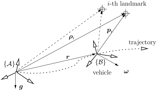
Figure 1: Coordinate frames for 3D localization of a vehicle.

As suggested in [36], we assume that the map is anchored to a set of $r$ landmarks observed at time $t=0$. Without loss of generality, we can say that the initial pose is given by $\bm{r}(0)=\bm{0}_{3\times 1}$ and $\bm{A}(0)=\bm{1}_{3}$. Thus

$$\bm{\rho}_{j}=\bm{p}_{j}(0)\qquad\forall j=1,\cdots,r.$$

The measurement vector includes the outputs of the landmark sensor, i.e.,

$$\bm{z}=\begin{bmatrix}\bm{p}_{1}\\ \vdots\\ \bm{p}_{m}\end{bmatrix}+\bm{v},$$ (4)

where vector $\bm{v}$ is landmark sensor noise which is assumed to be with covariance matrix

$$\bm{R}=E[\bm{v}\bm{v}^{T}].$$ (5)

As will be later discussed in Section 4.4, the Kalman filter tries to estimate the covariance matrix.

Since out of the set of $m$ landmarks there are $r$ known landmarks, there are $n=m-r$ landmarks with unknown position. Therefore, the entire state vector to be estimated is:

$$\bm{x}=[\bm{q}_{v}^{T}\;\bm{r}^{T}\;\dot{\bm{r}}^{T}\;\bm{b}_{g}^{T}\;\bm{b}_{a}^{T}\;\bm{\rho}_{r+1}^{T}\;\cdots\;\bm{\rho}_{m}^{T}]^{T}\in\mathbb{R}^{15+3n},$$ (6)

where $\bm{b}_{g}$ and $\bm{b}_{a}$ are the gyro and accelerometer biases as will be later discussed in the next section. In view of kinematic relations (2), we can rewrite (4) as a function of the states by

$$\bm{z}=\bm{h}(\bm{x})+\bm{v},$$ (7a)

where

$$\bm{h}(\bm{x})=\begin{bmatrix}{\bm{A}}^{T}(\bm{q})\big{(}\bm{\rho}_{1}-\bm{r}\big{)}\\ \vdots\\ {\bm{A}}^{T}(\bm{q})\big{(}\bm{\rho}_{n}-\bm{r}\big{)}\end{bmatrix}.$$ (7b)

constitutes the nonlinear observation model. To linearize the observation vector, we need to derive the sensitivity of the nonlinear observation vector with respect to the system variables. Consider small orientation perturbations

$$\delta\bm{q}=\bm{q}\otimes\bar{\bm{q}}^{*}.$$ (8)

around a nominal quaternion $\bar{\bm{q}}$—in the following, the bar sign stands for nominal value. Now, by virtue of $\bm{A}(\bm{q})=\bm{A}(\delta\bm{q}\otimes\bar{\bm{q}})$, one can compute the observation vector (7b) in terms of the perturbation $\delta\bm{q}$. Using the first order approximation of nonlinear matrix function $\bm{A}^{T}(\delta\bm{q})$ from expression (3) by assuming a small rotation $\delta\bm{q}$, i.e., $\|\delta\bm{q}_{v}\|\ll 1$ and $\delta q_{0}\approx 1$, we have

$$\bm{A}(\delta\bm{q})\approx\bm{1}_{3}+2[\delta\bm{q}_{v}\times].$$ (9)

Therefore, by the first-order approximation, the observation vector can be written as as the following bilinear function

$$\bm{h}=\begin{bmatrix}\big{(}\bm{1}_{3}-2[\delta\bm{q}_{v}\times]\big{)}\bar{\bm{A}}^{T}\big{(}\bm{\rho}_{1}-\bm{r}\big{)}\\ \vdots\\ \big{(}\bm{1}_{3}-2[\delta\bm{q}_{v}\times]\big{)}\bar{\bm{A}}^{T}\big{(}\bm{\rho}_{n}-\bm{r}\big{)}\end{bmatrix}+\text{HOT}.$$

Thus, the observation sensitivity matrix $\bm{H}=\left.\frac{\partial\bm{h}}{\partial\bm{x}}\right|_{\bm{A}=\bar{\bm{A}}}\in\mathbb{R}^{3m\times(15+3n)}$ can be written as

$$\bm{H}=\begin{bmatrix}2[\hat{\bm{p}}_{1}\times]&-\bar{\bm{A}}^{T}&\bm{0}_{3}&\bm{0}_{3}&\bm{0}_{3}&\bm{0}_{3}&\cdots&\bm{0}_{3}\\ \vdots&\vdots&\vdots&\vdots&\vdots&\vdots&\vdots&\vdots\\ 2[\hat{\bm{p}}_{r}\times]&-\bar{\bm{A}}^{T}&\bm{0}_{3}&\bm{0}_{3}&\bm{0}_{3}&\bm{0}_{3}&\cdots&\bm{0}_{3}\\ 2[\hat{\bm{p}}_{r+1}\times]&-\bar{\bm{A}}^{T}&\bm{0}_{3}&\bm{0}_{3}&\bm{0}_{3}&\bar{\bm{A}}^{T}&\cdots&\bm{0}_{3}\\ \vdots&\vdots&\vdots&\vdots&\vdots&\vdots&\ddots&\vdots\\ 2[\hat{\bm{p}}_{m}\times]&-\bar{\bm{A}}^{T}&\bm{0}_{3}&\bm{0}_{3}&\bm{0}_{3}&\bm{0}_{3}&\cdots&\bar{\bm{A}}^{T}\end{bmatrix}$$ (10)

where

$$\hat{\bm{p}}_{i}=\bar{\bm{A}}(\hat{\bm{\rho}}_{i}-\hat{\bm{r}})\qquad\forall i=1,\cdots m$$ (11)

are the estimation of the landmark positions calculated from the state estimation.

2.2 Motion Dynamics

Denoting the angular velocity of the vehicle by $\bm{\omega}$, the relation between the time derivative of the quaternion and the angular velocity can be readily expressed by

$$\dot{\bm{q}}=\frac{1}{2}\underline{\bm{\omega}}\otimes\bm{q}\quad\mbox{where}\quad\underline{\bm{\omega}}=\begin{bmatrix}\bm{\omega}\\ 0\end{bmatrix}$$ (12)

The angular rate is obtained from the rate gyro measurement

$$\bm{\omega}=\bm{\omega}_{g}+\bm{b}_{g}+\bm{\epsilon}_{g}$$ (13)

where $\bm{b}_{g}$ is the corresponding bias vector and $\bm{\epsilon}_{g}$ is the angular random walk noises with covariances $E[\bm{\epsilon}_{g}\bm{\epsilon}_{g}^{T}]=\sigma_{g}^{2}\bm{1}_{3}$. The gyro bias is modeled as

$$\dot{\bm{b}}_{g}=\bm{\epsilon}_{b_{g}},$$ (14)

where $\bm{\epsilon}_{b_{g}}$ is the random walk with covariances $E[\bm{\epsilon}_{b_{g}}\bm{\epsilon}_{b_{g}}^{T}]=\sigma_{b_{g}}^{2}\bm{1}_{3}$.

A measurement of the linear acceleration of the vehicle can be provided by an accelerometer. However, accelerometers cannot distinguish between the acceleration of gravity and inertial acceleration. Therefore, we must compensate the accelerometer output for the effects of gravity. Moreover, the accelerometer output $\bm{a}\in\mathbb{R}^{3}$ is accompanied by its own bias $\bm{b}_{a}$, which is modeled as $\dot{\bm{b}}_{a}=\bm{\epsilon}_{b_{a}}$ and $E[\bm{\epsilon}_{b_{a}}\bm{\epsilon}_{b_{a}}^{T}]=\sigma_{b_{a}}\bm{1}_{3}$. Thus, in the presence of a gravity field, the accelerometer output equation is represented by

$$\ddot{\bm{r}}=\bm{A}(\bm{q})\big{(}\bm{a}+\bm{b}_{a}+\bm{\epsilon}_{a}\big{)}-\bm{g},$$ (15)

where $\bm{a}$ is acceleration output, accelerometer noise $\bm{\epsilon}_{a}$ is the assumed to be random walk noise $\bm{\epsilon}_{a}$ with covariance $E[\bm{\epsilon}_{a}\bm{\epsilon}_{a}^{T}]=\sigma_{a}^{2}\bm{1}_{3}$, and $\bm{g}$ is the consrtant gravity vector expressed in the inertial frame $\{{\cal A}\}$.

Although the states can be propagated by solving the nonlinear dynamics equations (1), (12), (14) and (15), the state transition matrix of the linearized dynamics equations will be also needed to be used for covariance propagation of the KF. In order to linearize the equations, consider small position and orientation perturbations

$$\delta\bm{r} =\bm{r}-\bar{\bm{r}}$$ (16a)

$$\delta\bm{q} =\bm{q}\otimes\bar{\bm{q}}^{*}.$$ (16b)

Then, adopting a linearization technique similar to [49, 50] one can linearize (12) about the nominal quaternion $\bar{\bm{q}}$ and nominal velocity

$$\bar{\bm{\omega}}=\bm{\omega}_{g}+\bar{\bm{b}}_{g},$$

to obtain

$$\frac{\rm d}{{\rm d}t}\delta\bm{q}_{v}=-\bar{\bm{\omega}}\times\delta\bm{q}_{v}+\frac{1}{2}\delta\bm{b}_{g}+\frac{1}{2}\bm{\epsilon}_{g}.$$ (17)

Note that, since $\delta q_{o}$ is not an independent variable and it has variations of only the second order, its time derivative can be ignored, as suggested in [49].

Similarly, the equation of translational motion (15) can be linearized about the nominal trajectory obtained from

$$\ddot{\bar{\bm{r}}}=\bm{A}(\bar{\bm{q}})\bar{\bm{a}}-\bm{g},$$ (18)

where $\bar{\bm{a}}=\bm{a}+\bar{\bm{b}}_{a}$. Finally, using (9) in differentiation (16a) with respect to time yields

$$\frac{\rm d}{{\rm d}t}\delta\dot{\bm{r}} =\bm{A}(\delta\bm{q}\otimes\bar{\bm{q}})\big{(}\bar{\bm{a}}+\delta\bm{b}_{a}+\bm{\epsilon}_{a}\big{)}-\bm{A}(\bar{\bm{q}})\bar{\bm{a}}$$

$$\approx-2\bar{\bm{A}}[\bar{\bm{a}}\times]\delta\bm{q}_{v}+\bar{\bm{A}}\delta\bm{b}_{a}+\bar{\bm{A}}\bm{\epsilon}_{a},$$ (19)

where $\bar{\bm{A}}\triangleq\bm{A}(\bar{\bm{q}})$. Note that in derivation of (19), the second- and higher-order terms of $\delta\bm{q}_{v}$ are ignored. Then, assuming time-invariant parameters, one can assemble equations (1), (14), (17), and (19) in the standard state space form as

$$\delta\dot{\bm{x}}=\bm{F}\delta\bm{x}+\bm{G}\bm{\epsilon},$$ (20)

where vector $\bm{\epsilon}^{T}=[\bm{\epsilon}_{g}^{T}\;\bm{\epsilon}_{b_{g}}^{T}\;\bm{\epsilon}_{a}^{T}\;\bm{\epsilon}_{b_{a}}^{T}]\in\mathbb{R}^{12}$ contains the entire process noise; and

$$\bm{F}=\begin{bmatrix}-[\bar{\bm{\omega}}\times]&\bm{0}_{3}&\bm{0}_{3}&\frac{1}{2}\bm{1}_{3}&\bm{0}_{3}&\bm{0}_{3\times 3n}\\ \bm{0}_{3}&\bm{0}_{3}&\bm{1}_{3}&\bm{0}_{3}&\bm{0}_{3}&\bm{0}_{3\times 3n}\\ \bm{-}2\bar{\bm{A}}[\bar{\bm{a}}\times]&\bm{0}_{3}&\bm{0}_{3\times 3}&\bm{0}_{3}&\bar{\bm{A}}&\bm{0}_{3\times 3n}\\ &&&\bm{0}_{(6+3n)\times(15+3n)}&&\\ \end{bmatrix}$$ (21a)

$$\bm{G}=\begin{bmatrix}\frac{1}{2}\bm{1}_{3}&\bm{0}_{3}&\bm{0}_{3}&\bm{0}_{3}\\ \bm{0}_{3}&\bm{0}_{3}&\bm{0}_{3}&\bm{0}_{3}\\ \bm{0}_{3}&\bm{0}_{3}&\bar{\bm{A}}&\bm{0}_{3}\\ \bm{0}_{3}&\bm{1}_{3}&\bm{0}_{3}&\bm{0}_{3}\\ \bm{0}_{3}&\bm{0}_{3}&\bm{1}_{3}&\bm{0}_{3}\\ &\bm{0}_{3n\times 12}&\end{bmatrix}$$ (21b)

3 Observability

A successful use of Kalman filtering requires that the system be observable[51]. A linear time-invariant (LTI) systems is said to be globally observable if and only if its observability matrix is full rank. If a system is observable, the estimation error becomes only a function of the system noise, while the effect of the initial values of the states on the error will asymptotically vanish. The original observation model, (7), and a part of the process model, (12), are nonlinear systems. For nonlinear system, Hermann et al. proposed a rank condition test for “local weak observability” of nonlinear system that involves Lie derivative algebra [52]. Although this technique has been applied for observability of 2D SLAM [31], the analysis is too complex to be useful for the 3D case. The observability analysis can be simplified if the state-space is composed of the errors in terms of $\delta\bm{x}$. In that case, the time-varying system (10) and (20) can be replaced by a piecewise constant system for observability analysis [53, 46]. The intuitive motion is that such a time-varying system can be effectively approximated by a pieces-wise contact system without loosing the characteristic behavior of the original system [53, 54].

Now assume that $\bm{F}_{j}$ be $\bm{H}_{j}$ are the $j$th time segment of the system’s state transition matrix and observation model, respectively. Then, the observability matrix associated with linearized system (20) together with the observation model (10) is

$$\bm{{\cal O}}_{j}=\begin{bmatrix}\bm{H}_{j}^{T}&(\bm{H}_{j}\bm{F}_{j})^{T}&\cdots&(\bm{H}_{j}\bm{F}_{j}^{3n+14})^{T}\end{bmatrix}^{T}.$$

The states of the system is instantaneously observable if and only if

$$\mbox{rank}~{}\bm{{\cal O}}_{j}=3n+15$$ (22)

which is equivalent to $\bm{{\cal O}}_{j}$ having $3n+15$ independent rows. In the following analysis, we remove the index _j from the corresponding variables for the sake of simplicity of the notation. Now, we can construct the submatrices of the observability matrix as

$$\bm{H}\bm{F} =\begin{bmatrix}-2[\hat{\bm{p}}_{1}\times][\bar{\bm{\omega}}\times]&\bm{0}_{3}&-\bar{\bm{A}}^{T}&[\hat{\bm{p}}_{1}\times]&\bm{0}_{3}&\bm{0}_{3\times 3n}\\ \vdots&\vdots&\vdots&\vdots&\vdots&\vdots\\ -2[\hat{\bm{p}}_{m}\times][\bar{\bm{\omega}}\times]&\bm{0}_{3}&-\bar{\bm{A}}^{T}&[\hat{\bm{p}}_{m}\times]&\bm{0}_{3}&\bm{0}_{3\times 3n}\end{bmatrix}$$ (23a)

$$\bm{H}\bm{F}^{2} =\begin{bmatrix}2[\hat{\bm{p}}_{1}\times][\bar{\bm{\omega}}\times]^{2}+2[\bar{\bm{a}}\times]&\bm{0}_{3}&\bm{0}_{3}&-[\hat{\bm{p}}_{1}\times][\bar{\bm{\omega}}\times]&\bm{1}_{3}&\bm{0}_{3\times 3n}\\ \vdots&\vdots&\vdots&\vdots&\vdots&\vdots\\ 2[\hat{\bm{p}}_{m}\times][\bar{\bm{\omega}}\times]^{2}+2[\bar{\bm{a}}\times]&\bm{0}&\bm{0}&-[\hat{\bm{p}}_{m}\times][\bar{\bm{\omega}}\times]&\bm{1}_{3}&\bm{0}_{3\times 3n}\end{bmatrix}$$ (23b)

We consider the observability of the SLAM when there are three fixed landmarks, i.e., $r=3$. Then, as shown in the Appendix A, the following block-triangular matrix can be constructed from the observability matrix by few elementary Matrix Row Operations (MRO)

$$\small\bm{{\cal O}}\stackrel{{\scriptstyle\text{MRO}}}{{\longrightarrow}}\bm{{\cal O}}_{\Delta}\!\!=\!\!\begin{bmatrix}2\bm{\Pi}&\bm{0}_{3}&\bm{0}_{3}&\bm{0}_{3}&\bm{0}_{3}&\bm{0}_{3}&\cdots&\bm{0}_{3}\\ \times&-\bar{\bm{A}}^{T}&\bm{0}_{3}&\bm{0}_{3}&\bm{0}_{3}&\bm{0}_{3}&\cdots&\bm{0}_{3}\\ \times&\times&-\bar{\bm{A}}^{T}&\bm{0}_{3}&\bm{0}_{3}&\bm{0}_{3}&\cdots&\bm{0}_{3}\\ \times&\times&\times&\bm{\Pi}&\bm{0}_{3}&\bm{0}_{3}&\cdots&\bm{0}_{3}\\ \times&\times&\times&\times&\bm{1}_{3}&\bm{0}_{3}&\cdots&\bm{0}_{3}\\ \times&\times&\times&\times&\times&\bar{\bm{A}}^{T}&\cdots&\bm{0}_{3}\\ \times&\times&\times&\times&\times&\times&\ddots&\bm{0}_{3}\\ \times&\times&\times&\times&\times&\times&\times&\bar{\bm{A}}^{T}\end{bmatrix}.$$ (24)

where

$$\bm{\Pi}=[\bm{e}_{1}\times]^{2}+[\bm{e}_{2}\times]^{2},$$ (25)

is constructed from the landmark baseline vectors expressed in the vehicle frame as

$$\bm{e}_{i}=\frac{\hat{\bm{p}}_{i}-\hat{\bm{p}}_{3}}{\|\hat{\bm{p}}_{i}-\hat{\bm{p}}_{3}\|}\qquad i=1,2.$$ (26)

The block triangular matrix (24) is full rank if all of the block diagonal matrices are full rank. Therefore, the observability condition rests on showing that matrix $\bm{\Pi}$ is full-rank.

Proposition 1

If the three fixed landmarks are not place on a straight line, i.e.,

$$\bm{e}_{1}\times\bm{e}_{2}\neq\bm{0}$$ (27)

then matrix $\bm{\Pi}$ is full-rank and so is the observation matrix $\bm{{\cal O}}$.

Proof: In a proof by contradiction, we show that $\bm{\Pi}\in\mathbb{R}^{3\times 3}$ must be a full-rank matrix. If $\bm{\Pi}$ is not full-rank, then there must exist a non-zero vector $\bm{\lambda}\neq\bm{0}$ such that

$$\bm{\Pi}\bm{\lambda}=\bm{0}$$ (28)

In view of definition (25) and the following identity,

$$[\bm{e}_{i}\times]^{2}=\bm{e}_{i}\bm{e}_{i}^{T}-\|\bm{e}_{i}\|^{2}\bm{1}_{3},$$

one can easily show that (28) is equivalent to

$$\big{(}\bm{e}_{1}\bm{e}_{1}^{T}+\bm{e}_{2}\bm{e}_{2}^{T}\big{)}\bm{\lambda}=2\bm{\lambda}.$$ (29)

Since $\bm{e}_{1}\bm{e}_{1}^{T}$ and $\bm{e}_{2}\bm{e}_{2}^{T}$ are projection matrices to the subspace $\bm{e}_{1}$ and $\bm{e}_{2}$, respectively, the only possibility for the identity (29) to happen is that $\bm{e}_{1}\parallel\bm{e}_{2}\parallel\bm{\lambda}$. However, this is a contradiction because $\bm{e}_{1}$ and $\bm{e}_{2}$ are not parallel and therefore matrix $\bm{\Pi}$ must be full rank.

3.1 Observability of Piecewise Constant Equivalent

Now assume that $\bm{H}_{j}$ and $\bm{F}_{j}$ vary from segment $j=1$ to $j=r$. Then, the system (10)-(20) is to be completely observable if the total observability matrix

$$\tilde{\bm{{\cal O}}}=\begin{bmatrix}\bm{{\cal O}}_{1}\\ \bm{{\cal O}}_{1}e^{\bm{F}_{1}t_{\Delta_{1}}}\\ \vdots\\ \bm{{\cal O}}_{r}e^{\bm{F}_{r-1}t_{\Delta_{r-1}}}\cdots e^{\bm{F}_{1}t_{\Delta_{1}}}\end{bmatrix}$$ (30)

is full rank [53]. Moreover, if

$$\text{null}(\bm{{\cal O}}_{j})\subset\text{null}(\bm{F}_{j})\qquad\forall j=1,\cdots,r$$ (31)

then it has been shown that $\text{null}(\tilde{\bm{{\cal O}}})=\text{null}(\tilde{\bm{{\cal O}}}_{s})$, where

$$\tilde{\bm{{\cal O}}}_{s}\triangleq[\bm{{\cal O}}_{1}^{T}\;\cdots\;\bm{{\cal O}}_{r}^{T}]^{T}$$ (32)

is the stripped observability matrix [53]. If the condition (27) is satisfied, then the corresponding observability matrices are full rank, i.e., $\text{null}(\bm{{\cal O}}_{j})=\emptyset$. Consequently, condition (31) in trivially satisfied and the stripped observability matrix (32) is full rank. The above development can be summarized in the following Remark:

Remark 1

Assume that linearized system (10)-(20) is piecewise constant for every single segment $j=1,\cdots,r$. Then, the system during the time interval $t_{1}\leq t\leq t_{r}$ is completely observable if at least three known landmarks which are not placed in a straight line are observed

4 Adaptive SLAM

4.1 Discrete-Time Model

The equivalent discrete-time model of (20) is

$$\delta\bm{x}_{k+1}=\bm{\Phi}_{k}\delta\bm{x}_{k}+\bm{w}_{k}$$ (33)

where $\bm{\Phi}_{k}=\bm{\Phi}(t_{k},t_{\Delta})$ is the state transition matrix over time interval $t_{\Delta}=t_{k+1}-t_{k}$. In order to find a closed form solution for the state transition matrix, we need to have the nominal values of some of the states. Assuming that the nominal values of the bias parameters are obtained from the latest estimate update, i.e., $\bar{\bm{b}}_{g_{k}}=\hat{\bm{b}}_{g_{k}}$ and $\bar{\bm{b}}_{a_{k}}=\hat{\bm{b}}_{a_{k}}$, the nominal angular velocity and linear acceleration can be obtained by averaging the IMU signals at interval $t_{k}<t\leq t_{k}+t_{\Delta}$, i.e.,

$$\bar{\bm{\omega}}_{k} =\hat{\bm{b}}_{g_{k}}+\frac{1}{t_{\Delta}}\int_{t_{k}}^{t_{k}+t_{\Delta}}\bm{\omega}_{g}(\xi)d\xi$$ (34a)

$$\bar{\bm{a}}_{k} =\hat{\bm{b}}_{a_{k}}+\frac{1}{t_{\Delta}}\int_{t_{k}}^{t_{k}+t_{\Delta}}\bm{a}(\xi)d\xi\qquad 0<\tau\leq t_{\Delta}$$ (34b)

Then, the state transition matrix takes on the form:

$$\bm{\Phi}(t_{k},\tau)=\mbox{diag}\big{(}\bm{\Phi}^{\prime}(t_{k};\tau),\bm{1}_{3+3n}\big{)}$$

where

$$\bm{\Phi}^{\prime}(t_{k},\tau)=\begin{bmatrix}\bm{\Lambda}_{1_{k}}(\tau)&\bm{0}_{3}&\bm{0}_{3}&\frac{1}{2}\bm{\Lambda}_{2_{k}}(\tau)\\ \bm{0}_{3}&\bm{0}_{3}&\bm{1}_{3}\tau&\bm{0}_{3}\\ -\bar{\bm{A}}_{k}[\bar{\bm{a}}_{k}\times]\bm{\Lambda}_{2_{k}}(\tau)&\bm{0}_{3}&\bm{0}_{3}&\frac{1}{2}\bm{\Lambda}_{3_{k}}(\tau)\\ \bm{0}_{3}&\bm{0}_{3}&\bm{0}_{3}&\bm{1}_{3}\end{bmatrix}.$$

Here, $\bar{\bm{A}}_{k}\triangleq\bm{A}(\bar{\bm{q}}_{k})$ and the submatrices of the above matrix are given as

$$\bm{\Lambda}_{1_{k}}(\tau)= \bm{1}_{3}-\frac{\sin\varpi_{k}\tau}{\varpi_{k}}[\bar{\bm{\omega}}_{k}\times]+\frac{1-\cos\varpi_{k}\tau}{\varpi_{k}^{2}}[\bar{\bm{\omega}}_{k}\times]^{2}$$

$$\bm{\Lambda}_{2_{k}}(\tau)= \bm{1}_{3}\tau+\frac{\cos\varpi_{k}\tau-1}{\varpi_{k}^{2}}[\bar{\bm{\omega}}_{k}\times]+\frac{\varpi_{k}\tau-\sin\varpi_{k}\tau}{\varpi_{k}^{3}}[\bar{\bm{\omega}}_{k}\times]^{2}$$

$$\bm{\Lambda}_{3_{k}}(\tau)= \frac{1}{2}\bm{1}_{3}\tau^{2}+\frac{\sin\varpi_{k}\tau-\varpi_{k}\tau}{\varpi_{k}^{3}}[\bar{\bm{\omega}}_{k}\times]+\frac{\cos\varpi_{k}\tau+\frac{1}{2}\varpi_{k}^{2}\tau^{2}-1}{\varpi_{k}^{4}}[\bar{\bm{\omega}}_{k}\times]^{2},$$ (35)

where

$$\varpi_{k}\triangleq\|\bar{\bm{\omega}}_{k}\|.$$

Presumably, the continuous process noise of the entire system is with covariance

$$E[\bm{\epsilon}\;\bm{\epsilon}^{T}]=\bm{\Sigma}_{\epsilon}=\mbox{diag}(\sigma_{g}^{2}\bm{1}_{3},\sigma_{b_{g}}^{2}\bm{1}_{3},\sigma_{a}^{2}\bm{1}_{3},\sigma_{b_{a}}^{2}\bm{1}_{3}).$$

Then, the covariance matrix of the discrete-time process noise, which will be used by the KF, can be calculated from

$$\bm{Q}_{k} =E[\bm{w}_{k}\bm{w}_{k}^{T}]=\int_{t_{k}}^{t_{k}+t_{\Delta_{k}}}\bm{\Phi}(t)\bm{G}\bm{\Sigma}_{\epsilon}\bm{G}^{T}\bm{\Phi}^{T}(t){\rm d}t,$$ (36)

$$=\mbox{diag}\big{(}\bm{Q}^{\prime}_{k},\bm{0}_{(6+3n)\times(6+3n)}\big{)}$$

where $\bm{Q}^{\prime}_{k}$ is the nonzero sub-matrix of covariance matrix, which has the following structure

$$\bm{Q}^{\prime}_{k}=\begin{bmatrix}\bm{Q}^{\prime}_{k_{11}}&\times&\times&\times&\times\\ \bm{0}_{3}&\frac{1}{3}\sigma_{a}^{2}t_{\Delta}^{3}\bm{1}_{3}&\times&\times&\times\\ \bm{Q}^{\prime}_{k_{31}}&\bm{0}_{3}&\bm{Q}^{\prime}_{k_{33}}&\times&\times\\ \bm{Q}^{\prime}_{k_{41}}&\bm{0}_{3}&\bm{Q}^{\prime}_{k_{43}}&\sigma_{b_{g}}^{2}t_{\Delta}\bm{1}_{3}&\times\\ \bm{0}_{3}&\bm{0}_{3}&\bm{0}_{3}&\bm{0}_{3}&\sigma_{b_{a}}^{2}t_{\Delta}\bm{1}_{3}&\end{bmatrix}$$ (37)

Here the symmetric entries of the covariance matrix $\bm{Q}^{\prime}_{k}$ are not written for the sake of notation simplicity. For small angle

$$\theta_{k}=\varpi_{k}\tau\ll 1,\qquad 0\leq\tau\leq t_{\Delta}$$

we can say $\sin\theta_{k}\approx\theta_{k}-\frac{1}{6}\theta_{k}^{3}$ and $\cos\theta_{k}\approx 1-\frac{1}{2}\theta_{k}^{2}$. Consequently, using the Taylor expansion of the sinusoidal functions in the state transition matrix (35) and then substituting the reduced order matrix (given in Appendix B) into (36) and ignoring the third and higher-order terms of $\theta_{k}$ after integration will result in

$$\bm{Q}^{\prime}_{k_{11}} =\Big{(}\frac{\sigma_{g}^{2}}{4}t_{\Delta}+\frac{\sigma_{bg}^{2}}{12}t_{\Delta}^{3}\Big{)}\bm{1}_{3}+\frac{\sigma_{bg}^{2}}{240}t_{\Delta}^{5}[\bar{\bm{\omega}}_{k}\times]^{2}$$

$$\bm{Q}^{\prime}_{k_{31}} =\frac{\sigma_{b_{g}}^{2}}{32}t_{\Delta}^{4}\bm{1}_{3}-\frac{\sigma_{g}^{2}}{8}t_{\Delta}^{2}\bar{\bm{A}}_{k}[\bar{\bm{a}}_{k}\times]+\Big{(}\frac{\sigma_{b_{g}}^{2}}{240}t_{\Delta}^{5}\bm{1}_{3}-\frac{\sigma_{g}^{2}}{24}t_{\Delta}^{3}\bar{\bm{A}}_{k}[\bar{\bm{a}}_{k}\times]\Big{)}[\bar{\bm{\omega}}_{k}\times]$$

$$+\Big{(}\frac{\sigma_{b_{g}}^{2}}{576}t_{\Delta}^{6}\bm{1}_{3}-\frac{\sigma_{g}^{2}}{96}t_{\Delta}^{4}\bar{\bm{A}}_{k}[\bar{\bm{a}}_{k}\times]\Big{)}[\bar{\bm{\omega}}_{k}\times]^{2}$$

$$\bm{Q}^{\prime}_{k_{33}} =\frac{\sigma_{b_{g}}^{2}}{80}t_{\Delta}^{5}\bm{1}_{3}-\frac{\sigma_{b_{g}}^{2}}{12}t_{\Delta}^{3}[\bar{\bm{A}}_{k}\bar{\bm{a}}_{k}\times]+\frac{\sigma_{b_{g}}^{2}}{2016}t_{\Delta}^{7}[\bar{\bm{\omega}}_{k}\times]^{2}-\frac{\sigma_{g}^{2}}{240}t_{\Delta}^{5}\big{(}[\bar{\bm{A}}_{k}\bar{\bm{a}}_{k}\times][\bar{\bm{A}}_{k}\bar{\bm{\omega}}_{k}\times]\big{)}^{2}$$

$$\bm{Q}^{\prime}_{k_{41}} =\frac{\sigma_{b_{g}}^{2}}{4}t_{\Delta}^{2}\bm{1}_{3}+\frac{\sigma_{b_{g}}^{2}}{48}t_{\Delta}^{4}[\bar{\bm{\omega}}_{k}\times]^{2}$$

$$\bm{Q}^{\prime}_{k_{43}} =\frac{\sigma_{b_{g}}^{2}}{240}t_{\Delta}^{3}\Big{(}20\bm{1}_{3}+5t_{\Delta}[\bar{\bm{\omega}}_{k}\times]+t_{\Delta}^{2}[\bar{\bm{\omega}}_{k}\times]^{2}\Big{)}.$$

In the derivation of the above equations we use the following identities $\bar{\bm{A}}\bar{\bm{A}}^{T}=\bm{1}_{3}$ and $\bar{\bm{A}}[\bar{\bm{a}}\times]\bar{\bm{A}}^{T}=[(\bar{\bm{A}}\bar{\bm{a}})\times]$.

4.2 Estimator Design

Before we pay attention to the KF estimator design, it is important to point out that only the variation of the quaternion, $\delta\bm{q}_{v_{k}}$, and not the quaternion itself, $\bm{q}_{k}$, is estimated by the KF. Nevertheless, the full quaternion can be obtained from the former variables if the value of the nominal quaternion $\bar{\bm{q}}(t_{k})$ is given, i.e.,

$$\delta\hat{\bm{q}}_{k}^{-}=\hat{\bm{q}}_{k}^{-}\otimes\bar{\bm{q}}^{*}(t_{k})$$ (38)

For the linearization of the quaternion to make sense, the nominal quaternion trajectory, $\bar{\bm{q}}(t)$, should be close to actual one as much as possible. A natural choice for a posteriori nominal value of quaternion at $t_{k-1}$ is its update estimate, i.e., $\bar{\bm{q}}(t_{k-1})=\hat{\bm{q}}_{k-1}$. Since the nominal angular velocity $\bar{\bm{\omega}}_{k}$ is assumed constant at interval $t_{k-1}\leq t\leq t_{k}$, then according to (12) the nominal quaternion evolves from its initial value $\bar{\bm{q}}(t_{k-1})$ to its a priori value $\bar{\bm{q}}(t_{k})$ by

$$\bar{\bm{q}}_{k}\triangleq\bar{\bm{q}}(t_{k})=e^{\frac{t_{\Delta}}{2}[\underline{\bar{\bm{\omega}}}_{k}\otimes]}\hat{\bm{q}}_{k-1},$$ (39)

which will be used at the innovation step of KF. It can be shown that the above exponential matrix function has the following closed-form expression

$$e^{\frac{t_{\Delta}}{2}[\underline{\bar{\bm{\omega}}}_{k}\otimes]}=\big{(}\cos\frac{\varpi_{k}t_{\Delta}}{2}+\sin\frac{\varpi_{k}t_{\Delta}}{2}\big{)}\bm{1}_{4}+\Big{(}\frac{2}{\varpi_{k}t_{\Delta}}\sin\frac{\varpi_{k}t_{\Delta}}{2}-\frac{1}{2}\cos\frac{\varpi_{k}t_{\Delta}}{2}\Big{)}[\underline{\bar{\bm{\omega}}}_{k}\otimes]$$

The EKF-based observer for the associated noisy discrete system (33) is given in two steps: ($i$) estimate correction and ($ii$) estimation propagation. The estimate correction process begins by calculating the filter gain matrix as

$$\bm{K}_{k}=\bm{P}_{k}^{-}\bm{H}_{k}^{T}\big{(}\bm{H}_{k}\bm{P}_{k}^{-}\bm{H}_{k}^{T}+\bm{R}\big{)}^{-1}$$ (40a)

Next, the states of KF and the covariance matrix are updated in the innovation step. Recall that only the vector part of the quaternion variation, not the full quaternion, is included in the KF state vector. Therefore, we use a priori value of the nominal quaternion $$\bar{\bm{q}}_{k}\triangleq\bar{\bm{q}}(t_{k})$$ from expression (39) first to calculate the a priori quaternion deviation and then, after the state update in the innovation step, a posteriori quaternion deviation is recombined with the nominal quaternion to obtain the quaternion update. That is

$$\begin{bmatrix}\delta\hat{\bm{q}}_{v_{k}}\\ \hat{\bm{y}}_{k}\end{bmatrix}=\begin{bmatrix}\mbox{vec}(\hat{\bm{q}}_{k}^{-}\otimes\bar{\bm{q}}^{*}_{k})\\ \hat{\bm{y}}_{k}^{-}\end{bmatrix}+\bm{K}_{k}\big{(}\bm{z}_{k}-\bm{h}_{k}(\hat{\bm{x}}_{k}^{-})\big{)}$$ (40b)

$$\hat{\bm{q}}_{k}=\delta\hat{\bm{q}}_{k}\otimes\bar{\bm{q}}_{k}=\begin{bmatrix}\delta\hat{\bm{q}}_{v_{k}}\\ {\sqrt{1-\left\|\delta\hat{\bm{q}}_{v_{k}}\right\|^{2}}}\end{bmatrix}e^{\frac{t_{\Delta}}{2}[\underline{\bar{\bm{\omega}}}_{k}\otimes]}\hat{\bm{q}}_{k-1}$$ (40c)

Note that $\delta\hat{\bm{q}}_{v_{k}}^{-}=\mbox{vec}(\hat{\bm{q}}_{k}^{-}\otimes\bar{\bm{q}}^{*}_{k})$ in (40b) is a priori estimation of the quaternion deviation, where $\mbox{vec}(\cdot)$ returns the vector part of a quaternion. The process of quaternion update can be summarized as

$$\hat{\bm{q}}_{k}^{-}\stackrel{{\scriptstyle\eqref{eq:qbar_exp}}}{{\longrightarrow}}\delta\hat{\bm{q}}_{k}^{-}\stackrel{{\scriptstyle\eqref{eq:Innovation}}}{{\longrightarrow}}\delta\hat{\bm{q}}_{k}\stackrel{{\scriptstyle\eqref{eq:q_hat}}}{{\longrightarrow}}\hat{\bm{q}}_{k}$$

The covariance matrix is updated according to

$$\bm{P}_{k}=\big{(}\bm{1}_{15+3n}-\bm{K}_{k}\bm{H}_{k}\big{)}\bm{P}_{k}^{-},$$ (40d)

In the second step, the states and the covariance matrix are propagated into the next time step. Combining (12) and (15), we then describe the state-space model of the system as

$$\dot{\bm{x}}=\bm{f}(\bm{x},\bm{\epsilon}),$$

which can be used for estimating propagation of the states. Thus

$$\hat{\bm{x}}_{k+1}^{-} ={\hat{\bm{x}}_{k}}+\int_{t_{k}}^{t_{k}+t_{\Delta}}\bm{f}(\bm{x}(t),\bm{0})\,{\rm d}t$$ (41a)

$$\bm{P}_{k+1}^{-} =\bm{\Phi}_{k}\bm{P}_{k}\bm{\Phi}_{k}^{T}+\bm{Q}_{k}$$ (41b)

$$=\begin{bmatrix}\bm{\Phi}_{k}^{\prime}\begin{bmatrix}\bm{P}_{11}&\bm{P}_{12}^{T}\end{bmatrix}\bm{\Phi}_{k}^{\prime T}+\bm{Q}^{\prime}_{k}&\times\\ \begin{bmatrix}\bm{P}_{12}&\bm{P}_{22}\end{bmatrix}\bm{\Phi}_{k}^{\prime T}&\bm{P}_{22},\end{bmatrix},$$

where $\bm{P}_{11}\in\mathbb{R}^{12\times 12}$ and the other submatrices are obtained from adequate partitioning of the covariance matrix, i.e.,

$$\bm{P}=\begin{bmatrix}\bm{P}_{11}&\bm{P}_{12}^{T}\\ \bm{P}_{12}&\bm{P}_{22}\end{bmatrix}.$$

4.3 Initialization and Landmark Augmentation

Since the vehicle frame $\{{\cal B}\}$ coincides with inertial frames $\{{\cal A}\}$ at $t=0$, we can say $\bm{r}(0)=\bm{0}_{3\times 1}$ and $\bm{A}(0)=\bm{1}_{3}$. Moreover, since $\bm{z}(0)=\bm{\rho}(0)+\bm{v}$, the initial value of the states can be adequately chosen as

$$\bm{x}(0)=\begin{bmatrix}\bm{0}_{15\times 1}\\ \bm{z}(0)\end{bmatrix},\qquad\bar{\bm{A}}(0)=\bm{1}_{3},$$

while the initial value of the filter covariance matrix can be specified as

$$\bm{P}^{-}(0)=\begin{bmatrix}\bm{0}&\bm{0}\\ \bm{0}&\bm{R}(0)\end{bmatrix}$$

The KF estimation proceeds according to (40)-(41) cycle as long as the landmarks are reobserved. However, if a new landmark is observed then the KF states and its covariance matrix have to be augmented. Let us assume $\bm{z}_{\rm new}$ represent the observation associated with a new landmark at location $\bm{\rho}_{\rm new}$. Then, the explicit expression of the new landmark position can be obtained from the inverse kinematics of the observation as

$$\bm{\rho}_{\rm new} =\bm{A}(\delta\bm{q}\otimes\bar{\bm{q}})(\bm{z}_{\rm new}-\bm{v}_{\rm new})+\bm{r}$$

$$\approx\bar{\bm{A}}(\bm{1}_{3}+2[\delta{\bm{q}}_{v}\times])(\bm{z}_{\rm new}-\bm{v}_{\rm new})+\bm{r}$$

$$\approx\bar{\bm{A}}\bm{z}_{\rm new}+\hat{\bm{r}}\underbrace{-\bar{\bm{A}}\bm{v}_{\rm new}-2\bar{\bm{A}}[\bm{z}_{\rm new}\times]\delta\tilde{\bm{q}}_{v}+\tilde{\bm{r}}}_{\rm noise}$$

where $\tilde{\bm{q}}_{v}$ and $\tilde{\bm{r}}$ are the corresponding estimation errors and $\bm{R}_{\rm new}=E[\bm{v}_{\rm new}\bm{v}_{\rm new}^{T}]$. Consequently, the states and covariance matrix are augmented as

$$\hat{\bm{x}}_{\rm new}=\begin{bmatrix}\hat{\bm{x}}\\ \bar{\bm{A}}\bm{z}_{\rm new}+\hat{\bm{r}}\end{bmatrix}\quad\mbox{and}\quad\bm{P}_{\rm new}=\begin{bmatrix}\bm{P}&\bm{\Upsilon}^{T}\\ \bm{\Upsilon}&\bar{\bm{A}}\bm{R}_{\rm new}\bar{\bm{A}}^{T}\end{bmatrix}$$

where

$$\bm{\Upsilon}=\begin{bmatrix}-2\bar{\bm{A}}[\bm{z}_{\rm new}\times]&\bm{1}_{3}&\bm{0}_{3\times(9+3n)}\end{bmatrix}\bm{P}.$$

4.4 Noise-Adaptive Filter

Efficient implementation of the KF requires the statistical characteristics of the measurement noise [55, 56]. The IMU noises can be either derived from the sensor specification or empirically tuned. However, the landmark sensor noise is uncertain as they may vary from one point to the next. Therefore, it is desirable to weight camera measurement data in the fusion process heavily only when a “good” observation data is available. This requires readjusting the covariance matrix associated with $\bm{v}$ in the filter’s internal model based upon information obtained in real time from the measurements.

In a noise-adaptive Kalman filter, the issue is that, in addition to the states, the covariance matrix of the measurement noise has to be estimated [57, 58]. Let us define the residual error

$$\bm{\varrho}_{k}\triangleq\bm{z}_{k}-\bm{H}_{k}\hat{\bm{x}}_{k}^{-}.$$

Then the following identity holds

$$\bm{\varrho}_{k}=\bm{H}_{k}(\hat{\bm{x}}_{k}-\hat{\bm{x}}_{k}^{-})+\bm{v}_{k}.$$

Taking variance of on both sides of the above equation gives

$$\bm{R}_{k}=\bm{W}_{k}-\bm{H}_{k}\bm{P}_{k}^{-}\bm{H}_{k}^{T}\quad\mbox{with}\quad\bm{W}_{k}=E[\bm{\varrho}_{k}\bm{\varrho}_{k}^{T}]$$

The above equation can be used to estimate the measurement covariance matrix $\hat{\bm{R}}_{k}$ from an ergodic approximation of the covariance of the zero-mean residual $\bm{\varrho}$ in the sliding sampling window with length $w$. That is

$$\hat{\bm{W}}_{k} \approx\frac{1}{w}\sum_{i=k-w}^{k}\bm{\varrho}_{i}\bm{\varrho}_{i}^{T}$$ (42a)

$$=\hat{\bm{W}}_{k-1}+\frac{1}{w}\Big{(}\bm{\varrho}_{k}\bm{\varrho}_{k}^{T}-\bm{\varrho}_{k-w}\bm{\varrho}_{k-w}^{T}\Big{)}.$$ (42b)

where $w$ is chosen empirically to give some statistical smoothing.

5 A Case Study

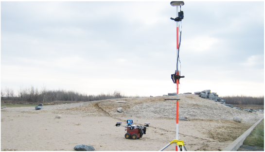
Figure 2: CSA Mars emulation terrain.

A series of case studies were conducted on the CSA’s red-rover traversing the $30~{}\times~{}60$ m Mars Emulation Terrain (MET), as shown in Fig. 2, in order to demonstrate the convergence property of the 3D SLAM with respect to different numbers of fixed landmarks. The rover is equipped with IMU plus three RTK GPS antennas, which allows to measure not only the vehicle position but also its attitude using the method described in [9]. Consequently, the vehicle pose trajectories obtained from the GPS system are considered as the “ground-truth” path.

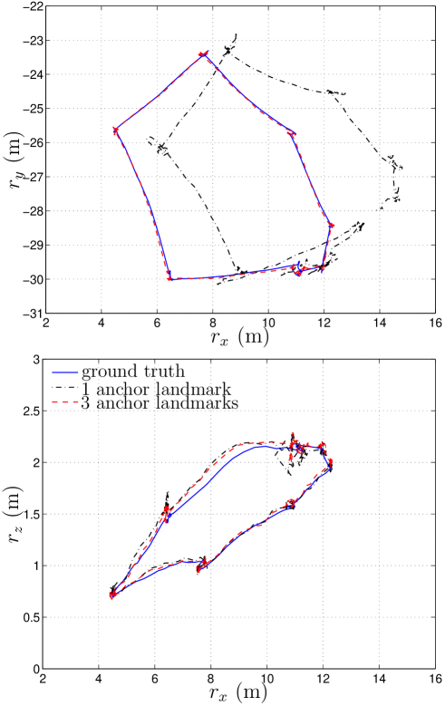
Figure 3: 3D path taken by the vehicle.

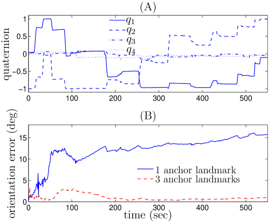
Figure 4: Estimation of vehicle attitude.

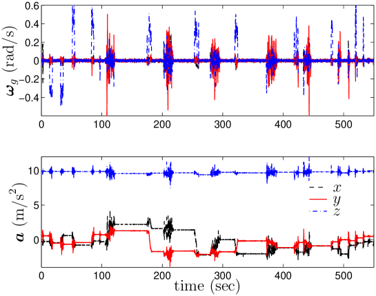
Figure 5: IMU outputs.

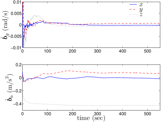
Figure 6: Estimation of the IMU calibration parameters.

Figs. 3 and 4A show the 3D path taken by the mobile robot and its attitude, respectively, while the vehicle passing through seven via points. The IMU measurements are received at the rate of 20 Hz, and the corresponding trajectories are depicted in Figs. 5. In this case study, the relative positions of the landmarks are simulated by using the ground truth trajectories and a set of random noise sequences with difference standard deviations bounded by $0.1<\sigma_{p_{i}}<0.25$ (m). The filter processed the data from three scenarios as: (i) one of the observed landmarks used as a global reference, (ii) three of the observed landmarks used as a global reference. Figs. 3 shows trajectories of the position estimates for the two cases, while the corresponding orientation estimate errors are shown in 4B. Here, the orientation errors is calculated by

$$\text{Orientation Error}=2\sin^{-1}\|\text{vec}(\hat{\bm{q}}^{*}\otimes\bm{q}_{\rm ref})\|.$$ (43)

It is evident from the graphs that the filter did not converge if only one of the first observed landmark is used as the global reference. However, the results clearly show that the pose estimates very well converges to the actual values if three of the observed landmarks are used as the global references. Fig. 6 illustrates the time history of the estimates of the gyroscope bias and the accelerometer bias.

6 Conclusions

Development and the corresponding observability analysis of an adaptive SLAM by fusing IMU and landmark sensors for autonomous driving vehicles have been presented. Examining the observability of such SLAM technique in 3-dimensional environment led to the conclusion that the system is observable if at least three known landmarks which are not placed in a straight line are observed. The IMU calibration parameters and the covariance matrix of measurement noise associated with landmark sensors were estimated upon the sensor information obtained in real time so that the adaptive estimator is continuously “tuned” as well as possible.

Appendix A Reducing $\bm{{\cal O}}$ Through Matrix Row Operations

The following matrix

$$\small\bm{{\cal O}}\stackrel{{\scriptstyle\text{MRO}}}{{\longrightarrow}}\begin{bmatrix}2[(\hat{\bm{p}}_{1}-\hat{\bm{p}}_{3})\times]&\bm{0}_{3}&\bm{0}_{3}&\bm{0}_{3}&\bm{0}_{3}&\bm{0}_{3}&\cdots&\bm{0}_{3}\\ 2[(\hat{\bm{p}}_{2}-\hat{\bm{p}}_{3})\times]&\bm{0}_{3}&\bm{0}_{3}&\bm{0}_{3}&\bm{0}_{3}&\bm{0}_{3}&\cdots&\bm{0}_{3}\\ \times&-\bar{\bm{A}}^{T}&\bm{0}_{3}&\bm{0}_{3}&\bm{0}_{3}&\bm{0}_{3}&\cdots&\bm{0}_{3}\\ \times&\times&-\bar{\bm{A}}^{T}&[\hat{\bm{p}}_{1}\times]&\bm{0}_{3}&\bm{0}_{3}&\cdots&\bm{0}_{3}\\ \times&\times&\bm{0}_{3}&[(\hat{\bm{p}}_{1}-\hat{\bm{p}}_{3})\times]&\bm{0}_{3}&\bm{0}_{3}&\cdots&\bm{0}_{3}\\ \times&\times&\bm{0}_{3}&[(\hat{\bm{p}}_{2}-\hat{\bm{p}}_{3})\times]&\bm{0}_{3}&\bm{0}_{3}&\cdots&\bm{0}_{3}\\ \times&\times&\times&\times&\bm{1}_{3}&\bm{0}_{3}&\cdots&\bm{0}_{3}\\ \times&\times&\times&\times&\times&\bar{\bm{A}}^{T}&\cdots&\bm{0}_{3}\\ \times&\times&\times&\times&\times&\times&\ddots&\bm{0}_{3}\\ \times&\times&\times&\times&\times&\times&\times&\bar{\bm{A}}^{T}\end{bmatrix}$$ (44)

can be constructed via the following elementary operations: The first and second rows of the above matrix are obtained by subtracting the third row from the first and second rows of matrix $\bm{H}$, (10). Performing the same operation in matrix $\bm{H}\bm{F}$, in (23a), produces the fifth and sixth rows of the above matrix. The third, forth, seventh rows are picked from first rows of matrices $\bm{H}$, $\bm{H}\bm{F}$, and $\bm{H}\bm{F}^{2}$, respectively. The last rows of the above matrix are picked from the $r+1$th to the $m$th rows of matrix $\bm{H}$. Now, pre-multiplying the first and second rows of (44) by $[\bm{e}_{1}\times]/\|\hat{\bm{p}}_{1}-\hat{\bm{p}}_{3}\|$ and $[\bm{e}_{2}\times]/\|\hat{\bm{p}}_{2}-\hat{\bm{p}}_{3}\|$, respectively, and the adding the resultant rows and performing similar operations on the fifth and sixth rows of (44) yields

$$\small\begin{bmatrix}2\bm{\Pi}&\bm{0}_{3}&\bm{0}_{3}&\bm{0}_{3}&\bm{0}_{3}&\bm{0}_{3}&\cdots&\bm{0}_{3}\\ \times&-\bar{\bm{A}}^{T}&\bm{0}_{3}&\bm{0}_{3}&\bm{0}_{3}&\bm{0}_{3}&\cdots&\bm{0}_{3}\\ \times&\times&-\bar{\bm{A}}^{T}&[\hat{\bm{p}}_{1}\times]&\bm{0}_{3}&\bm{0}_{3}&\cdots&\bm{0}_{3}\\ \times&\times&\bm{0}_{3}&\bm{\Pi}&\bm{0}_{3}&\bm{0}_{3}&\cdots&\bm{0}_{3}\\ \times&\times&\times&\times&\bm{1}_{3}&\bm{0}_{3}&\cdots&\bm{0}_{3}\\ \times&\times&\times&\times&\times&\bar{\bm{A}}^{T}&\cdots&\bm{0}_{3}\\ \times&\times&\times&\times&\times&\times&\ddots&\bm{0}_{3}\\ \times&\times&\times&\times&\times&\times&\times&\bar{\bm{A}}^{T}\end{bmatrix}.$$ (45)

Finally, pre-multiplying the forth row of (45) by $-[\hat{\bm{p}}_{1}\times]\bm{\Pi}^{-1}$ and then add the resultant row to the third row of (45) yields (24).

Appendix B Simplified $\bm{\Lambda}_{i}$s’

$$\bm{\Lambda}_{1_{k}}(\tau)\approx \bm{1}_{3}-\tau[\bar{\bm{\omega}}_{k}\times]+\frac{\tau^{2}}{2}[\bar{\bm{\omega}}_{k}\times]^{2}$$ (46)

$$\bm{\Lambda}_{2_{k}}(\tau)\approx \bm{1}_{3}\tau-\frac{\tau^{2}}{2}[\bar{\bm{\omega}}_{k}\times]+\frac{\tau^{3}}{6}[\bar{\bm{\omega}}_{k}\times]^{2}$$

$$\bm{\Lambda}_{3_{k}}(\tau)\approx \bm{1}_{3}\frac{\tau^{2}}{2}-\frac{\tau^{3}}{6}[\bar{\bm{\omega}}_{k}\times]+\frac{\tau^{4}}{24}[\bar{\bm{\omega}}_{k}\times]^{2}$$

References

- [1] F. Aghili, “3d simultaneous localization and mapping using IMU and its observability analysis,” Journal of Robotica, December 2010.
- [2] B. Barshan and H. F. Durrant-Whyte, “Inertial navigation systems for mobile robots,” IEEE Trans. on Robotics & Automation, vol. 11, no. 3, pp. 328–342, June 1995.
- [3] F. Aghili and A. Salerno, Multisensor Attitude Estimation and Applications, 1st ed. CRC Press, 2016, ch. Adaptive Data Fusion of Multiple Sensors for Vehicle Pose Estimation.
- [4] J. Vaganay, M. J. Aldon, and A. Fournier, “Mobile robot attitude estimation by fusion of inertial data,” in IEEE Int. Conference on Robotics & Automation, Atlanta, GA, May 1993, pp. 277–282.
- [5] F. Aghili and A. Salerno, “Driftless 3D attitude determination and positioning of mobile robots by integration of IMU with two RTK GPSs,” IEEE/ASME Trans. on Mechatronics, vol. 18, no. 1, pp. 21–31, Feb. 2013.
- [6] G. Dissanayake, S. Sukkarieh, E. Nebot, and H. Durrant-Whyte, “The aiding of a low-cost strapdown inertial measurement unit using vehicle model constraints for land vehicle applications,” IEEE Trans. on Robotics & Automation, vol. 17, no. 5, pp. 731–747, 2001.
- [7] F. Aghili and A. Salerno, “3-D localization of mobile robots and its observability analysis using a pair of RTK GPSs and an IMU,” in IEEE/ASME Int. Conf. on Advanced Intelligent Mechatronics (AIM), Montreal, Canada, July 2010, pp. 303–310.
- [8] H.-S. Choi, O.-D. Park, and H.-S. Kim, “Autonomous mobile robot using GPS,” in Int. Conference on Control & Automation, Budapest, Hungary, June 2005, pp. 858–862.
- [9] F. Aghili and A. Salerno, “Attitude determination and localization of mobile robots using two RTK GPSs and IMU,” in IEEE/RSJ International Conference on Intelligent Robots & Systems, St. Louis, USA, October 2009, pp. 2045–2052.
- [10] D. Strelow and S. Singh, “Online motion estimation from image and inertial measurements,” in Int. Conference on Advanced Robotics, Portugal, June 30–July 3 2003.
- [11] F. Aghili and K. Parsa, “Motion and parameter estimation of space objects using laser-vision data,” AIAA Journal of Guidance, Control, and Dynamics, vol. 32, no. 2, pp. 538–550, March 2009.
- [12] A. Mallet, S. Lacroix, and L. Gallo, “Position estimation in outdoor environments using pixel tracking and stereovision,” in IEEE Int. Conference on Robotics & Automation, San Francisco, CA, April 2000, pp. 3519–3524.
- [13] F. Aghili, M. Kuryllo, G. Okouneva, and C. English, “Fault-tolerant position/attitude estimation of free-floating space objects using a laser range sensor,” IEEE Sensors Journal, vol. 11, no. 1, pp. 176–185, Jan. 2011.
- [14] P. Lamon and R. Siegwart, “3d position tracking in challenging terrain,” The Int. Journal of Robotics Research, vol. 26, no. 2, pp. 167–186, February 2007.
- [15] F. Aghili and C. Y. Su, “Robust relative navigation by integration of icp and adaptive kalman filter using laser scanner and imu,” IEEE/ASME Transactions on Mechatronics, vol. 21, no. 4, pp. 2015–2026, Aug 2016.
- [16] A. I. Mourikis, N. Trawny, S. I. Roumeliotis, D. M. Helmick, and L. Matthies, “Autonomous stair climbing for tracked vehicles,” The Int. Journal of Robotics Research, vol. 26, no. 7, pp. 737–758, July 2007.
- [17] F. Aghili, “Automated rendezvous & docking (AR&D) without impact using a reliable 3d vision system,” in AIAA Guidance, Navigation and Control Conference, Toronto, Canada, August 2010.
- [18] F. Aghili, M. Kuryllo, G. Okouneva, and C. English, “Fault-tolerant pose estimation of space objects,” in IEEE/ASME Int. Conf. on Advanced Intelligent Mechatronics (AIM), Montreal, Canada, July 2010, pp. 947–954.
- [19] F. Aghili, K. Parsa, and E. Martin, “Robotic docking of a free-falling space object with occluded visual condition,” in 9th Int. Symp. on Artificial Intelligence, Robotics & Automation in Space, Los Angeles, CA, Feb. 26 – 29 2008.
- [20] F. Aghili, M. Kuryllo, G. Okuneva, and D. McTavish, “Robust pose estimation of moving objects using laser camera data for autonomous rendezvous & docking,” in ISPRS Worksshop Laserscanning, Paris, France, September 2009, pp. 253–258.
- [21] F. Aghili and K. Parsa, “Adaptive motion estimation of a tumbling satellite using laser-vision data with unknown noise characteristics,” in 2007 IEEE/RSJ International Conference on Intelligent Robots and Systems, Oct 2007, pp. 839–846.
- [22] R. Smith, M. Self, and P. Cheesman, Estimating Uncertain Spatial Relationship in Robotics, Autonomous Robot Vehicle, I. Cox and G. Wilfong, Eds. New York: Springer-Verlag, 1987.
- [23] H. F. Durant-Whyte, “Uncertain geometry in robotics,” IEEE Trans. on Robotics & Autimation, vol. 4, no. 1, pp. 23–31, 1988.
- [24] N. Ayache and O. Faugeras, “Maintaining a representation of the environment of a mobile robot,” IEEE Trans. on Robotics & Automation, vol. 5, no. 6, pp. 804–819, 1998.
- [25] J. J. Leonard and H. F. Durrant-Whyte, “Simultaneous map building and localization for an autonomous mobile robot,” in IEEE/RSJ Int. Workshop on Intelligent Robots and Systems, Osaka, Japan, November 1991, pp. 1442–1447.
- [26] T. Bailey and H. Durrant-Whyte, “Simultaneous localization and mapping (SLAM): Part II,” IEEE Robotics & Automation Magazine, vol. 13, no. 3, pp. 108–117, September 2006.
- [27] B. Xi, R. Guo, F. Sun, and Y. Huang, “Simulation research for active simultaneous localization and mapping based on extended kalman filter,” in IEEE/RSJ Int. Conference on Intelligent Robots and Systems, Qingdao, China, September 2008, pp. 2443–2448.
- [28] H. Rehbinder and B. K. Ghosh, “Pose estimation using line-based dynamic vision and inertial sensors,” IEEE Transactions on Automatic Control, vol. 48, no. 2, pp. 186–199, Feb. 2003.
- [29] J. Thienel and R. M. Sanner, “A coupled nonlinear spacecraft attitude controller and observer with an unknown constant gyro bias and gyro noise,” IEEE Transactions on Automatic Control, vol. 48, no. 11, pp. 2011–2015, November 2003.
- [30] J. Vasconcelos, R. Cunha, C. Silvestre, and P. Oliveira, “Landmark based nonlinear observer for rigid body attitude and position estimation,” in Decision and Control, 2007 46th IEEE Conference on, 12-14 2007, pp. 1033 –1038.
- [31] K. W. L. amd W. S. Wijesoma and J. I. Guzman, “On the observability and observability analysis of SLAM,” in IEEE/RSJ Int. Conference on Intelligent Robots and Systems, Beijing, China, October 2006, pp. 3569–3574.
- [32] L. Perera, A. Melkumyan, and E. Nettleton, “On the linear and nonlinear observability analysis of the slam problem,” in Mechatronics, 2009. ICM 2009. IEEE International Conference on, 14-17 2009, pp. 1 –6.
- [33] “Robust adaptive observers for nonlinear systems with bounded disturbances,” in R. Marino and G. L. Santosuesso and P. Tomei, vol. 5, 1999, pp. 5200–5205.
- [34] Q. Zhang, “Adaptive observer for multiple-input-multiple-output (mimo) linear time-varying systems,” Automatic Control, IEEE Transactions on, vol. 47, no. 3, pp. 525–529, mar. 2002.
- [35] Z. Chen, K. Jiang, and J. C. Hung, “Local observability matrix and its application to observability analysis,” in 16th Annual Conference of IEEE (IECON’90), Pacific Grove, CA, USA, November 1990, pp. 100–103.
- [36] J. Andrade-Cetto and A. Sanfeliu, “The effects of partial observability when building fully correlated maps,” IEEE Trans. on Robotics & Autimation, vol. 21, no. 4, pp. 771–777, 2005.
- [37] S. Huang and G. Dissanayake, “Convergence analysis for extended kalman filter based SLAM,” in IEEE Int. Conf. on Robotics & Automation, Orlando, Florida, May 2006, pp. 1556–1563.
- [38] G. P. Huang, A. I. Mourikis, and S. I. Roumeliotis, “Analysis and improvement of consistency of extended kalman filter based SLAM,” in IEEE Int. Conf. on Robotics & Automation, Pasadena, CA, May 2008, pp. 473–479.
- [39] H. Surmann, A. Nuchter, K. Lingemann, and J. Hetzberg, “6D SLAM - preliminary report on closing the loop in six dimension,” in Proceedings of the 5th IFAC/EURON Symposium on Intelligent Autonomous Vehicles (IVA), Lisbon, Portugal, July 2004.
- [40] J. Kim and A. Sukkarieh, “Autonomous airborne navigation in unknown terrain environment,” IEEE Trans. on Aerospace & Electronic Systems, vol. 40, no. 3, pp. 1031–1045, July 2004.
- [41] J. Weingarten and R. Siegwart, “EKF-based 3D SLAM for structured environment reconstruction,” in IEEE/RSJ Int. Conference on Intelligent Robots and Systems, Edmonton, Canada, 2005, pp. 2089–2094.
- [42] D. M. Cole and P. Newman, “Using laser range data for 3D SLAM in outdoor environment,” in IEEE Int. Conf. on Robotics & Automation, Orlando, Florida, May 2006, pp. 1556–1563.
- [43] A. Nuechter, K. Lingemann, J. Hertzberg, and H. Surmann, “6D SLAM-?mapping outdoor environment,” in IEEE Int. Workshop of Safety, Security and Rescue Robotics, Gaithersburg, Maryland USA, August 2006.
- [44] J. Kim and S. Sukkarieh, “Real-time implementation of airborne inertial-SLAM,” Robotics and Autonomous Systems, vol. 55, no. 1, pp. 519–535, 2007.
- [45] S. Abdallah, D. Asmar, and J. Zelek, “A benchmark for outdoor SLAM systems,” Journal of Field Robotics, vol. 24, no. 1-2, pp. 145–165, 2007.
- [46] M. Bryson and S. Sukkarieh, “Observability analysis and active control for airborne slam,” Aerospace and Electronic Systems, IEEE Transactions on, vol. 44, no. 1, pp. 261–280, january 2008.
- [47] Z. Liu, Z. Hu, and K. Uchimura, “SLAM estimation in dynamic outdoor environment: A review,” Lecture Notes in Computer Science, vol. 5928, 2009.
- [48] A. Nemra and N. Aouf, “Robust airborne 3D visual simultaneous localization and mapping with observability and consistency analysis,” Journal of Intelligent and Robotic Systems, vol. 55, no. 4–5, pp. 345–376, 2009.
- [49] E. J. Lefferts, F. L. Markley, and M. D. Shuster, “Kalman filtering for spacecraft attitude estimation,” vol. 5, no. 5, pp. 417–429, Sep.–Oct. 1982.
- [50] M. E. Pittelkau, “Kalman filtering for spacecraft system alignment calibration,” vol. 24, no. 6, pp. 1187–1195, Nov. 2001.
- [51] F. Aghili, “Integrating IMU and landmark sensors for 3D SLAM and the observability analysis,” in Proc. of IEEE/RSJ International Conference on Intelligent Robots and Systems (IROS), Taipei, Taiwan, Oct. 2010, pp. 2025–2032.
- [52] R. Hermann and A. Krener, “Nonlinear controllability and observability,” Automatic Control, IEEE Transactions on, vol. 22, no. 5, pp. 728 – 740, oct 1977.
- [53] D. Goshen-Meskin and I. Y. Bar-Itzhack, “Observability analysis of piece-wise constant systems. i. theory,” Aerospace and Electronic Systems, IEEE Transactions on, vol. 28, no. 4, pp. 1056 –1067, oct 1992.
- [54] F. Aghili, “3D SLAM using IMU and its observability analysis,” in IEEE Int. Conf. on Mechatronics and Automation (ICMA), Xian, China, August 2010, pp. 377–383.
- [55] F. Aghili, M. Kuryllo, G. Okouneva, and C. English, “Robust vision-based pose estimation of moving objects for automated rendezvous & docking,” in IEEE Int. Conf. on Mechatronics and Automation (ICMA), Xian, China, August 2010, pp. 305–311.
- [56] F. Aghili and K. Parsa, “An adaptive vision system for guidance of a robotic manipulator to capture a tumbling satellite with unknown dynamics,” in IEEE/RSJ Int. Conf. on Intelligent Robots and Systems, Nice, France, September 2008, pp. 3064–3071.
- [57] P. S. Maybeck, Stochastic Models, Estimation, and Control (Volume 2). New York: Academic Press, 1982.
- [58] C. K. Chui and G. Chen, Kalman Filtering with Real-Time Applications. Berlin: Springer, 1998, pp. 113–115.