Abstract

We investigate the tachyonic instability of Kerr-Newman (KN) black holes in the Einstein-Maxwell-scalar (EMS) theory with a positive coupling parameter $\alpha$. This corresponds to exploring the onset of spontaneous scalarization for KN black holes. For this purpose, we use the hyperboloidal foliation method (HFM) to solve the linearized scalar equation numerically. We obtain a 3D graph [$\log_{10}\alpha(a,Q)$] which indicates the onset surface for spontaneous scalarization of KN black holes in the EMS theory. We find that there is no lower bound on the rotational parameter $a$, but its upper bound is given by $M^{2}-Q^{2}\geq a^{2}$. Also, we confirm that the high rotation enhances spontaneous scalarization of KN black holes in the EMS theory.

1 Introduction

In general relativity (GR), the “no-hair theorem” has been always a hot topic. This theorem allows that a GR black hole can be described by three observables of mass $M$, electric charge $Q$, and rotation parameter $a=J/M$ [1, 2]. The no-hair theorem rules out black holes coupled to a scalar field in asymptotically flat spacetimes due to the divergent scalar on the horizon and instability of the scalar [3, 4, 5]. However, one may circumvent no-hair theorems by violating some of their assumptions. We remind the reader that Damour and Esposito-Farese [6] has first found a new mechanism of spontaneous scalarization to obtain a scalarized black hole in the scalar-tensor theory with nonminimal scalar coupling. Recently, in two scalar-tensor theories which include the nonminimal coupling of a scalar to either the Gauss-Bonnet (GB) term [7, 8, 9] or Maxwell term [10], the scalar field has triggered destabilization of static (scalar-free) black holes and induced scalarized (charged) black holes. In those cases, the tachyonic instability leads to occurrence of spontaneous scalarization phenomenon for the black holes in GR.

More recently, the phenomenon of spontaneous scalarization of spinning black holes has been attracted to the readers in two scalar-tensor theories. First, Dima et al. [11] have found that the high rotation can induce tachyonic instability of Kerr black hole by evaluating the $(1+1)$ scalar evolution equation in the Einstein-scalar-Gauss-Bonnet (ESGB) theory with a positive coupling. When choosing a negative coupling parameter, it is known that an upper $a$-bound [$a/M\geq 0.5$] comes out as the onset of scalarization for Kerr black holes, but the low rotation ($a/M<0.5$) is supposed to suppress spontaneous scalarization. Shortly afterward, the critical rotation parameter $(a/M)_{c}=0.5$ for Kerr black holes was computed analytically [12] and numerically [13, 14, 15] in the ESGB theory with negative coupling parameters. In this direction, spin induced scalarized black holes have been also constructed numerically in the ESGB theory with positive coupling parameter [16, 17, 18]. Zou and Myung et al. [19] and Doneva et al. [20] have discussed spontaneous scalarization of Kerr black holes by including two different coupling functions. This means that the rotation parameter $a$ and the coupling parameter $\alpha$ play an important role in achieving spontaneous scalarization of spinning black holes.

Very recently, we have investigated the spontaneous scalarization for Kerr-Newman (KN) black holes in the Einstein-Maxwell-scalar (EMS) theory with a negative coupling parameter $\alpha$  [21]. We prefer the Maxwell coupling to scalar than the GB coupling in the KN black holes background because the former gives a simpler potential term than the latter. We have obtained an $a$-bound $(a/r_{+}\geq\hat{a}=0.4142)$ in the limit of $\alpha\rightarrow-\infty$ by using an analytical method [22]. The threshold curves [$\alpha(a)$] were found with different charge $Q$, describing the boundary between bald KN and scalarized KN black holes in the EMS theory. These curves indicated the critical rotation parameter $\hat{a}=0.4142$ clearly. This explains how spin-charge induced scalarization arises from the EMS theory with the negative coupling parameter.

In the present work, we wish to complete the analysis of the phenomenon for spontaneous scalarization of KN black holes by considering a positive coupling parameter in the EMS theory. We use the hyperboloidal foliation method (HFM) to solve the linearized scalar equation numerically. It is found that there is no lower bound on $a$, compared to the case of a negative coupling parameter. Instead, we find the upper bound on $a$ ($M^{2}-Q^{2}\geq a^{2}$) as the existence condition for the outer horizon. Importantly, we obtain a 3D graph [$\log_{10}\alpha(a,Q)$] which indicates the onset surface for spontaneous scalarization of KN black holes clearly in the EMS theory. In addition, we confirm that the high rotation enhances spontaneous scalarization of KN black holes in the EMS theory. Our action of the EMS theory takes the form  [10]

$$S_{\rm EMS}=\frac{1}{16\pi}\int d^{4}x{\sqrt{-g}\Big{[}R-2\partial_{\mu}\phi\partial^{\mu}\phi-f(\phi)F_{\mu\nu}F^{\mu\nu}\Big{]}}.$$ (1)

Here, the coupling function $f(\phi)$ is important to control a nonminimal coupling of scalar $\phi$ to Maxwell term $F_{\mu\nu}F^{\mu\nu}\equiv F^{2}$ with $F_{\mu\nu}=\partial_{\mu}A_{\nu}-\partial_{\nu}A_{\mu}$. We will probe the tachyonic instability of KN black holes by adopting hyperboloidal foliation method. In this case, we do not need to worry about the sophisticated outer boundary problem [23, 24], since the ingoing (outgoing) boundary condition at the horizon (infinity) to solve the linearized scalar equation will be satisfied automatically.

We organize the present work as follows. In Sec. 2, we revisit briefly the linearized scalar equation in the EMS theory. Then, we study the spin-charge induced scalarization of KN black holes in Sec. 3. The Sec. 4 is devoted to contributing to conclusions and discussions.

2 Linearized scalar equation

The variation of action (1) with respect to the metric $g_{\mu\nu}$, scalar field $\phi$, and vector potential $A_{\mu}$ gives the following equations:

$$R_{\mu\nu}-\frac{1}{2}Rg_{\mu\nu}=2\partial_{\mu}\phi\partial_{\nu}\phi-(\partial\phi)^{2}g_{\mu\nu}+2f(\phi)\Big{(}F_{\mu\rho}F_{\nu}~{}^{\rho}-\frac{F^{2}}{4}g_{\mu\nu}\Big{)},$$ (2)

$$\nabla_{\mu}\nabla^{\mu}\phi-\frac{1}{4}\frac{df(\phi)}{d\phi}F^{2}=0,$$ (3)

$$\partial_{\mu}\left(\sqrt{-g}f(\phi)F^{\mu\nu}\right)=0.$$ (4)

For a coupling function $f(\phi)$, its form has to accommodate a GR black hole in the limit of $\phi\rightarrow 0$ (namely, KN black holes in the Einstein-Maxwell gravity).

To discuss the tachyonic instability of black holes in EMS theory, we consider the linearized perturbation equation

$$\left(\bar{\square}-\mu_{\rm eff}^{2}\right)\delta\phi=0,\quad\mu_{\rm eff}^{2}=\frac{F^{2}}{4}\frac{d^{2}f}{d\phi^{2}}(0).$$ (5)

This instability is characterized by the presence of a negative mass term ($\mu^{2}_{\rm eff}<0)$ in the linearized scalar equation. Until now, many authors adopted different forms of coupling function $f(\phi)$, such as exponential coupling form $e^{\alpha\phi^{2}}$ [10], quadratic coupling form $1+\alpha\phi^{2}$ [25], hyperbolic cosine coupling form $\cosh\sqrt{2\alpha}\phi$ [26], and so on. Without loss of generality, we do not choose any precise form of coupling function $f(\phi)$ and only require that $f(\phi)$ satisfy [26, 27]

$$f(0)=1,\quad\frac{df}{d\phi}(0)=0,\quad\frac{d^{2}f}{d\phi^{2}}(0)=2\alpha.$$ (6)

Therefore, it will make our model more general in the investigation for spontaneous scalarization of KN black holes in EMS theory.

Without scalar hair, the axisymmetric KN black hole is expressed in terms of the Boyer-Lindquist coordinates as

$$ds^{2}_{\rm KN} \equiv \bar{g}_{\mu\nu}dx^{\mu}dx^{\nu}=-\frac{\Delta-a^{2}\sin^{2}\theta}{\rho^{2}}dt^{2}-\frac{2a\sin^{2}\theta(r^{2}+a^{2}-\Delta)}{\rho^{2}}dtd\varphi$$ (7)

$$+\frac{[(r^{2}+a^{2})^{2}-\Delta a^{2}\sin^{2}\theta]\sin^{2}\theta}{\rho^{2}}d\varphi^{2}+\frac{\rho^{2}}{\Delta}dr^{2}+\rho^{2}d\theta^{2},$$

where

$$\Delta=r^{2}-2Mr+a^{2}+Q^{2},\quad\rho^{2}=r^{2}+a^{2}\cos^{2}\theta.$$

The corresponding vector potential is

$$A=-\frac{Qr}{\rho^{2}}\left(dt-a\sin^{2}\theta d\varphi\right).$$ (8)

Then, the outer and inner horizons are obtained by imposing $\Delta=(r-r_{+})(r-r_{-})=0$ as

$$r_{\pm}=M\pm\sqrt{M^{2}-a^{2}-Q^{2}},$$ (9)

where one requires the existence condition for the outer horizon ($M^{2}-Q^{2}\geq a^{2}$). For simplicity, we set the mass of KN black hole to be $M=1$ in the whole article.

We shall compute the tachyonic instability of KN black holes in the EMS theory. Considering Eqs.(5),(6), and (8), the effective mass squared is obtained as

$$\mu_{\rm eff}^{2}=-\frac{\alpha Q^{2}(r^{4}-6a^{2}r^{2}\cos^{2}\theta+a^{4}\cos^{4}\theta)}{\left(r^{2}+a^{2}\cos^{2}\theta\right)^{4}}.$$ (10)

Under the scalar perturbation with $\alpha>0$, the KN black holes may become unstable in the presence of $\mu^{2}_{\rm eff}<0$.

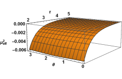
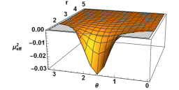
Figure 1: Two 3D graphs for the effective mass term ($\mu^{2}_{\rm eff}$) with $\alpha=1$, $M=1$, and $Q=0.3$. These include $r\in[r_{+},5]$ and $\theta\in[0,\pi]$. Left: a graph for $a=0.1$ and $r_{+}=1.95$ shows whole negative region. Right: a graph for $a=0.9$ and $r_{+}=1.32$ represents negative region around $\theta=\pi/2$ with small positive regions at $\theta=0$ and $\pi$.

Intuitively, the influence of an effective mass term $\mu^{2}_{\rm eff}$ on the tachyonic instability of KN black holes could be understood from its profiles. From Fig. 1, one observes that a graph of $\mu^{2}_{\rm eff}$ with $a=0.1$ shows a whole negative region, while a graph for $a=0.9$ represents a negative region around $\theta=\pi/2$ [$\mu^{2}_{\rm eff}=-Q^{2}/r^{4}$ for the Reissner-Nordström (RN) case] and maintains positive near $\theta=0,\pi$. It appears that the negative region in the $\theta$ direction decreases as $a$ increases. One observes from Fig. 1 that for $\alpha=1$, $\mu_{\rm eff}^{2}(r=r_{+},Q=0.3,a=0.9,\theta=\pi/2)=-0.03$ is $20\times\mu_{\rm eff}^{2}(r=r_{+},Q=0.3,a=0.1,\theta=\pi/2)=-0.006$. Therefore, one conjectures that the high rotation enhances spontaneous scalarization. In the chargeless limit of $Q\to 0$, one finds $\mu^{2}_{\rm eff}\to 0$ (a massless scalar propagation). However, its specific form of threshold curve [$\log_{10}\alpha(a,Q)$] will be determined only after performing numerical computations for a very long time.

3 Spin-charge induced scalarization

Before proceeding, we mention that it is not easy to solve the partial differential equation (5) directly. In our previous work [21], we adopted the $(2+1)$-dimensional hyperboloidal foliation method to solve the linearized scalar equation numerically with negative coupling parameter. It is worth noting that the time evolution of a linearized scalar is independent of the sign of coupling parameter $\alpha$. Hence, we adopt this method to explore the evolution of the linearized scalar with positive coupling parameter. Using two coordinate transformations and introducing the auxiliary fields

$$\Psi_{m}=\partial_{R}u_{m},\quad\Pi_{m}=\partial_{T}u_{m},$$ (11)

three coupled first-order differential equations are given by [21]

$$\partial_{T}u_{m}=\Pi_{m},$$ (12)

$$\partial_{T}\Psi_{m}=\partial_{T}\partial_{R}u_{m}=\partial_{R}\Pi_{m},$$ (13)

$$\partial_{T}\Pi_{m}=-(\tilde{B}^{T}\Pi_{m}+\tilde{A}^{TR}\partial_{R}\Pi_{m}+\tilde{A}^{RR}\partial_{R}\Psi_{m}+\tilde{A}^{\theta\theta}\partial_{\theta}^{2}u_{m}$$

$$\qquad\qquad+\tilde{B}^{R}\Psi_{m}+\tilde{B}^{\theta}\partial_{\theta}u_{m}+\tilde{C}u_{m}).$$ (14)

Here $R$ and $T$ are the compactified radial and suitable time coordinates in the hyperboloidal foliation method, respectively. More details of the derivation and the coefficients of the above equations can be found in Appendix A.

Now the spatial part of differential equations will be solved by making use of the finite difference method and the time evolution can be explored by using the fourth-order Runge-Kutta integrator. In particular, the ingoing (outgoing) boundary conditions at the outer horizon (infinity) are satisfied automatically in $R$ direction on account of the Racz and Toth coordinates. So we do not need to set the ingoing (outgoing) boundary conditions. For boundary conditions in the $\theta$ direction, the coefficients of Eq. (14) become singular at $\theta=0$ and $\theta=\pi$. Therefore, to implement these conditions  [21, 28, 29], we adopt a staggered grid and add ghost points as

$$u_{m}(T,R,\theta)=u_{m}(T,R,-\theta),$$

$$u_{m}(T,R,\pi+\theta)=u_{m}(T,R,\pi-\theta),\quad{\rm for}\quad m=0,\pm 2,\cdots$$ (15)

and

$$u_{m}(T,R,\theta)=-u_{m}(T,R,-\theta),$$

$$u_{m}(T,R,\pi+\theta)=-u_{m}(T,R,\pi-\theta),\quad{\rm for}\quad m=\boldsymbol{1},\pm 3,\cdots.$$ (16)

During numerical computation, we compute the equation in a domain $(R_{+},1)\times(0,\pi)$ with grids of $201\times 68$ in the $R$ and $\theta$ directions.

As the initial perturbation, we choose a spherically harmonic Gaussian distribution centered at $R_{c}$ outside the outer horizon

$$u_{lm}(T=0,R,\theta)\sim Y_{lm}(\theta,0)e^{-\frac{(R-R_{c})^{2}}{2\sigma^{2}}},$$ (17)

where $Y_{lm}(\theta,\phi)$ represent the spherical harmonic functions and $\sigma$ is the width of Gaussian distribution. In the following, we take $R_{c}=\frac{R_{+}+1}{2}$ with $R_{+}=\frac{\sqrt{r_{+}^{2}+1}-1}{r_{+}}$ and $\sigma=\frac{1}{\sqrt{200}}$. Also, we set $M=1$ so that all quantities are measured in units of $M$. It points out that although there is one initial mode with a specified $l$ only, other $l$ modes with the same index $m$ will be activated during evolving processes. The $l=m$ mode will have a dominant contribution at late times. For example, we can evaluate the processes of time evolution for several modes with $m=0$ and different $l$ numbers, and found that the late-time dominant mode is always the mode with $l=m=0$, see Fig. 2. Actually, a similar phenomenon has also occurred for Kerr black holes [14, 28] and KN black holes [21]. Hereafter, we consider axisymmetric perturbations with $l=m=0$ only for simplicity.

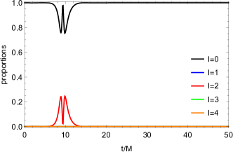
(a) $m=0$, initial mode $l=0$

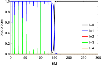
(b) $m=0$, initial mode $l=1$

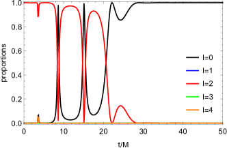
(c) $m=0$, initial mode $l=2$

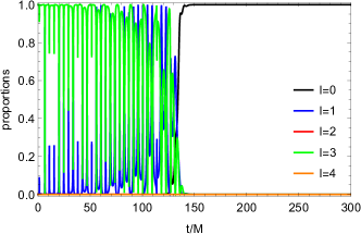
(d) $m=0$, initial mode $l=3$

Figure 2: Several modes with $m=0$ and different $l$ numbers are activated by the initial $l$ mode during the process of time evolution. Here the initial mode is specified to be the one with (a)$l=0$, (b) 1, (c) 2 and (d) 3, respectively. It is found that the dominant mode is always the $l=m=0$ mode at late enough time, whatever initial mode is chosen.

Considering different coupling parameter $\alpha$, the time-domain profiles of the $l=m=0$ mode for a linearized scalar are plotted in Fig. 3. The $\alpha=21$ case represents the threshold (marginal) evolution of instability.

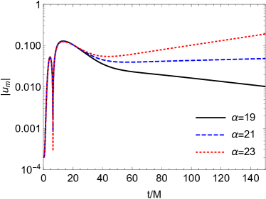
Figure 3: Time-domain profiles of a linearized scalar $|u_{m}|$ for $Q=0.4$ and $a=0.9$ with $M=1$ and different coupling constants $\alpha$.

Furthermore, we make the marginal curves with different charge $Q$, rotation parameter $a$, and coupling parameter $\alpha$ for a fixed mode $m=0$. We find that the tachyonic instability of KN black holes happens only in a certain region of the parameter space (see Fig. 4). Choosing $Q=0.2$, for example, the threshold curve [$\log_{10}\alpha(a)$] starts at $\log_{10}\alpha=\log_{10}141.041(=2.149)$ on the $\alpha$ axis, corresponding to the threshold of unstable RN black holes [25]. It determines the right boundary in the $\log_{10}\alpha(a)$ graph [Fig. 4].

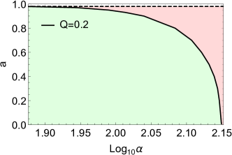
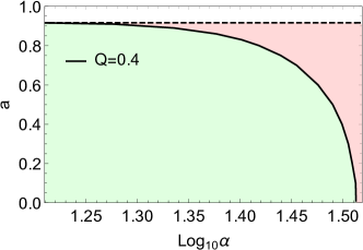
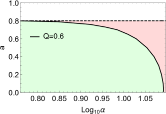
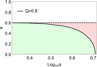
Figure 4: Four threshold curves [$\log_{10}\alpha(a)$] for the dominant $m=0$ mode with (a)$Q=0.2$ ,(b)0.4, (c)0.6 and (d)0.8, and $M=1$. The solid lines denote the boundaries between stable (green) and unstable (red) region. The dashed lines represent the existence condition ($M^{2}-Q^{2}\geq a^{2}$) of the outer horizon.

In this case, the instability can be only achieved in the region ($\log_{10}\alpha\geq 2.149$), and this threshold curve decreases from 2.149 to a smaller value as $a$ increases from 0 to 0.980 (upper bound) with $Q=0.2$. Here, the upper bound (denoted by dashed line) is determined by the existence condition of the outer horizon ($M^{2}-Q^{2}\geq a^{2}$). For $Q=0.2$, 0.4, 0.6 and 0.8, the maximum values (upper bound) of $a$ are given by 0.980, 0.917, 0.8 and 0.6, respectively. We note that the upper bound on $a$ also decreases as charge $Q$ increases. Importantly, we find from Fig. 4 that for all fixed $Q$ and $\alpha$, there exist unstable scalar modes for the points in the region (red) above the threshold curve and the KN black holes become unstable in this region. On the other hand, for points in the region (green) below the threshold curve, there are no growing modes and the KN black holes are stable.

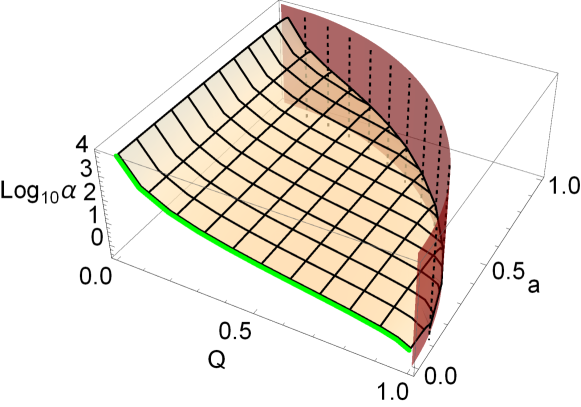
Figure 5: The 3D threshold graph [$\log_{10}\alpha(a,Q)$] as function of rotation parameter $a$ and charge $Q$. The orange surface denotes the onset surface of spin-charge induced scalarization for KN black holes in the EMS theory. The brown boundary represents the existence condition of outer horizon ($M^{2}-Q^{2}\geq a^{2}$) and the green curve indicates the threshold curve for the unstable RN black holes.

In Fig. 5, we obtain a 3D graph [$\log_{10}\alpha(a,Q)$] which indicates the onset surface of spin-charge induced scalarization for KN black holes in the EMS theory. The brown boundary is constructed by combining all dashed lines shown in Fig. 4, which represents the existence condition for the outer horizon ($M^{2}-Q^{2}\geq a^{2})$. The orange surface depicts the boundary between the stable (lower) region and unstable (upper) regions. In the nonrotating limit of $a\rightarrow 0$, this surface reduces to the green curve, which represents the threshold curve of tachyonic instability for RN black holes [25]. In the chargeless limit of $Q\to 0(\mu^{2}_{\rm eff}\to 0)$, one recovers a massless scalar propagation around the Kerr black holes, which turns out to be stable because there is no room for the unstable region. This picture indicates the onset of spontaneous scalarization for the KN black holes in the EMS theory clearly.

On the other hand, we also try to adopt the $(2+1)$ time evolution method to recalculate the late-time tails of the perturbed scalar field to perform the tachyonic instability of the KN black holes numerically in the time domain, as shown in Appendix B. The late-time tails in Fig. 6 demonstrate that it serves as an independent check of the previous results.

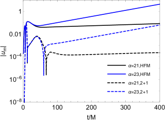
Figure 6: The time-domain profiles $(m=0)$ of scalar perturbation with $Q=0.4$, $M=1$, $a=0.9$, and different values of $\alpha$ by using two different numerical methods. This figure implies that the late-time tails of perturbed scalar fields share the same behaviors.

4 Conclusions and discussions

In this work, we have carried out the tachyonic instability of KN black holes in the EMS theory with a positive scalar coupling to Maxwell term. We adopted the hyperboloidal compactification technique to calculate the $(2+1)$-dimensional evolution of an initial linearized scalar located outside the outer horizon numerically. Consequently, we have obtained the 3D threshold curve [$\log_{10}\alpha(a,Q)$] which describes a boundary surface between stable (lower region) and unstable (upper region) KN black holes. Moreover, the high rotation enhances spontaneous scalarization. Also, the threshold curve decreases rapidly as $a$ increases and hits the $\alpha$ axis in the nonrotating limit of $a\rightarrow 0$. The computation including nonlinear effects are expected to quench the tachyonic instability and lead to constructing scalarized KN black holes.

Before finishing, we wish to mention some prospects of this work. Recently, Doneva et al. [30] investigated the spin induced scalarization of Kerr black hole in the ESGB theory with a massive scalar, and then Zhang [31] has discussed the Kerr black hole in the dynamical Chern-Simons gravity with a massive scalar. It is interesting to generalize our work by introducing a massive scalar. There may be richer physics involved in studying of the dynamics and the fate of the KN black holes. In addition, another promising direction is to construct the scalarized KN black holes in the EMS theory explicitly.

Acknowledgments

This work is supported by National Key R$\&$D Program of China (Grant No. 2020YFC2201400). D. C. Z acknowledges financial support from Outstanding Young Teacher Programme from Yangzhou University, No. 137050368. M. Y. L acknowledges financial support from the Initial Research Foundation of Jiangxi Normal University.

Appendix A

In this appendix, we will show how to transform the scalar field perturbation equation (5) into a form suitable for numerical calculations. This mainly contains two coordinate transformations, which have the advantages that the time slices are horizon penetrating and connect to future null infinity such that no boundary conditions are needed.

First, we rewrite the KN metric (7) in the ingoing Kerr-Schild coordinates $\{\tilde{t},r,\theta,\tilde{\varphi}\}$ by applying the coordinate transformations

$$d\tilde{t}=dt+\frac{2Mr-Q^{2}}{\Delta}dr,\quad d\tilde{\varphi}=d\varphi+\frac{a}{\Delta}dr.$$ (18)

and it becomes

$$ds^{2} = -\left(1-\frac{2Mr-Q^{2}}{\rho^{2}}\right)d\tilde{t}^{2}-\frac{2a\left(2Mr-Q^{2}\right)\sin^{2}\theta}{\rho^{2}}d\tilde{t}d\tilde{\varphi}+\frac{4Mr-2Q^{2}}{\rho^{2}}d\tilde{t}dr$$ (19)

$$+\left(1+\frac{2Mr-Q^{2}}{\rho^{2}}\right)dr^{2}-2a\sin^{2}\theta\left(1+\frac{2Mr-Q^{2}}{\rho^{2}}\right)drd\tilde{\varphi}+\rho^{2}d\theta^{2}$$

$$+\left(r^{2}+a^{2}+\frac{(2Mr-Q^{2})a^{2}\sin^{2}\theta}{\rho^{2}}\right)\sin^{2}\theta d\tilde{\varphi}^{2}.$$

Given the axial symmetry of the KN geometry, the perturbative variable $\delta\phi$ can be decomposed as

$$\delta\phi(\tilde{t},r,\theta,\tilde{\varphi})=\frac{1}{r}\sum_{m}u_{m}(\tilde{t},r,\theta)e^{im\tilde{\varphi}}.$$ (20)

Substituting the above ansatz into Eq. (5), the scalar perturbation equation in the ingoing Kerr-Schild coordinates takes the following form

$$A^{\tilde{t}\tilde{t}}\partial_{\tilde{t}}^{2}u_{m}+A^{\tilde{t}r}\partial_{\tilde{t}}\partial_{r}u_{m}+A^{rr}\partial^{2}_{r}u_{m}$$

$$+A^{\theta\theta}\partial_{\theta}^{2}u_{m}+B^{\tilde{t}}\partial_{\tilde{t}}u_{m}+B^{r}\partial_{r}u_{m}+B^{\theta}\partial_{\theta}u_{m}+Cu_{m}=0$$ (21)

with coefficients

$$A^{\tilde{t}\tilde{t}}=\rho^{2}+2Mr-Q^{2},~{}~{}A^{\tilde{t}r}=2Q^{2}-4Mr,~{}~{}A^{rr}=-\Delta,~{}~{}A^{\theta\theta}=-1,$$

$$B^{\tilde{t}}=2M-\frac{2Q^{2}}{r},~{}~{}B^{r}=\frac{2}{r}(a^{2}+Q^{2}-Mr)-2ima,~{}~{}B^{\theta}=-\cot\theta,$$

$$C=\frac{m^{2}}{\sin^{2}\theta}-\frac{2(a^{2}+Q^{2}-Mr)}{r^{2}}+\frac{2ima}{r}+\mu^{2}_{\rm eff}\rho^{2}.$$ (22)

As the second step, it is helpful to introduce the compactified radial coordinate $R$ and the suitable time coordinate $T$ following Racz and Toth [32] with

$$\tilde{t}=T+h(R),\quad r=R/\Omega(R),$$ (23)

where the height function $h(R)$ and conformal factor $\Omega(R)$ are given by

$$h(R)=\frac{1+R^{2}}{1-R^{2}}-4M\ln(1-R^{2}),\quad\Omega(R)=\frac{1-R^{2}}{2}.$$ (24)

As the result of the conformal transformation (23), Eq. (21) becomes

$$\partial^{2}_{T}u_{m}+\tilde{A}^{TR}\partial_{T}\partial_{R}u_{m}+\tilde{A}^{RR}\partial^{2}_{R}u_{m}$$

$$+\tilde{A}^{\theta\theta}\partial_{\theta}^{2}u_{m}+\tilde{B}^{T}\partial_{T}u_{m}+\tilde{B}^{R}\partial_{R}u_{m}+\tilde{B}^{\theta}\partial_{\theta}u_{m}+\tilde{C}u_{m}=0,$$ (25)

where coefficients can be expressed with

$$\{\tilde{A}^{TR},\tilde{A}^{RR},\tilde{A}^{\theta\theta},\tilde{B}^{T},\tilde{B}^{R},\tilde{B}^{\theta},\tilde{C}\}=\frac{1}{A^{TT}}\{A^{TR},A^{RR},A^{\theta\theta},B^{T},B^{R},B^{\theta},C\}$$ (26)

and

$$A^{TT}=A^{\tilde{t}\tilde{t}}-HA^{\tilde{t}r}+H^{2}A^{rr},$$

$$B^{T}=B^{\tilde{t}}-HB^{r}-\frac{(1-R^{2})^{2}}{2(1+R^{2})}H^{\prime}A^{rr},$$

$$A^{RR}=\left(\frac{(1-R^{2})^{2}}{2(1+R^{2})}\right)^{2}A^{rr},$$

$$A^{TR}=\frac{(1-R^{2})^{2}}{2(1+R^{2})}A^{\tilde{t}r}-\frac{(1-R^{2})^{2}}{1+R^{2}}HA^{rr},$$

$$B^{R}=\frac{(1-R^{2})^{2}}{2(1+R^{2})}\left[B^{r}+\left(\frac{(1-R^{2})^{2}}{2(1+R^{2})}\right)^{\prime}A^{rr}\right],$$ (27)

where the prime denotes the derivative $\frac{d}{dR}$ and $H(R)=\frac{dh}{dr}(R)$.

Finally, by introducing the following auxiliary fields

$$\Psi_{m}=\partial_{R}u_{m},$$ (28)

$$\Pi_{m}=\partial_{T}u_{m},$$ (29)

one finds the following coupled equations:

$$\partial_{T}u_{m}=\Pi_{m},$$ (30)

$$\partial_{T}\Psi_{m}=\partial_{T}\partial_{R}u_{m}=\partial_{R}\Pi_{m},$$ (31)

$$\partial_{T}\Pi_{m}=-(\tilde{B}^{T}\Pi_{m}+\tilde{A}^{TR}\partial_{R}\Pi_{m}+\tilde{A}^{RR}\partial_{R}\Psi_{m}+\tilde{A}^{\theta\theta}\partial_{\theta}^{2}u_{m}$$

$$\qquad\qquad+\tilde{B}^{R}\Psi_{m}+\tilde{B}^{\theta}\partial_{\theta}u_{m}+\tilde{C}u_{m}),$$ (32)

which are first order in space and time.

Appendix B

We will calculate the late-time tails of a perturbed scalar field to perform the tachyonic instability of the KN black holes numerically in the time domain. For the linearized scalar equation (5), we introduce a new coordinate $\varphi^{*}$ and tortoise coordinate $x$ through the transformations [31]

$$d\varphi^{*} = d\varphi+\frac{a}{\Delta}dr,$$

$$dx = \frac{r^{2}+a^{2}}{\Delta}dr.$$ (33)

Then we have a scalar field perturbed equation

$$\left[(r^{2}+a^{2})^{2}-\Delta a^{2}\sin^{2}\theta\right]\partial^{2}_{t}\delta\phi-(r^{2}+a^{2})^{2}\partial_{x}^{2}\delta\phi-2r\Delta\partial_{x}\delta\phi$$

$$+2a\left(2Mr-Q^{2}\right)\partial_{t}\partial_{\varphi^{*}}\delta\phi-2a(r^{2}+a^{2})\partial_{x}\partial_{\varphi^{*}}\delta\phi-\frac{\Delta}{\sin\theta}\partial_{\theta}(\sin\theta\partial_{\theta}\delta\phi)$$

$$-\frac{\Delta}{\sin^{2}\theta}\partial^{2}_{\varphi^{*}}\delta\phi+\Delta\left(r^{2}+a^{2}\cos^{2}\theta\right)\mu_{\rm eff}^{2}\delta\phi=0,$$ (34)

where the coordinate $x\in(-\infty,\infty)$ covers the infinite range which is accessible to an observer located outside the outer horizon, while one notes the semi-infinite region $r\in[r_{+},\infty)$ when using the radial coordinate $r$.

Taking into account the axial symmetry of (7), the scalar perturbation could be decomposed as

$$\delta\phi(t,x,\theta,\varphi^{*})=\sum_{m}\delta\phi(t,x,\theta)e^{im\varphi^{*}}$$ (35)

with $m$ as an azimuthal number. Substituting (35) into (34), we have a (2+1)-dimensional equation

$$\left[(r^{2}+a^{2})^{2}-\Delta a^{2}\sin^{2}\theta\right]\partial^{2}_{t}\delta\phi-(r^{2}+a^{2})^{2}\partial^{2}_{x}\delta\phi-\Delta\partial^{2}_{\theta}\delta\phi$$

$$+2ima{(2Mr-Q^{2})}\partial_{t}\delta\phi-2\left[r\Delta+ima(r^{2}+a^{2})\right]\partial_{x}\delta\phi-\Delta\cot{\theta}\partial_{\theta}\delta\phi$$

$$+\Delta\Big{[}(r^{2}+a^{2}\cos^{2}\theta)\mu_{\rm eff}^{2}+\frac{m^{2}}{\sin^{2}\theta}\Big{]}\delta\phi=0.$$ (36)

We may rewrite (36) as the (2+1)-dimensional Teukolsky equation

$$\partial^{2}_{t}\delta\phi+A^{xx}\partial^{2}_{x}\delta\phi+A^{\theta\theta}\partial^{2}_{\theta}\delta\phi+B^{t}\partial_{t}\delta\phi+B^{x}\partial_{x}\delta\phi+B^{\theta}\partial_{\theta}\delta\phi+C\delta\phi=0$$ (37)

whose coefficients take the forms

$$A^{tt} = \left[(r^{2}+a^{2})^{2}-\Delta a^{2}\sin^{2}\theta\right],$$

$$A^{xx} = -\frac{(r^{2}+a^{2})^{2}}{A^{tt}},$$

$$A^{\theta\theta} = -\frac{\Delta}{A^{tt}},$$

$$B^{t} = \frac{2ima{(2Mr-Q^{2})}}{A^{tt}},$$

$$B^{x} = -\frac{2r\Delta+2ima(r^{2}+a^{2})}{A^{tt}},$$

$$B^{\theta} = -\frac{\Delta\cot{\theta}}{A^{tt}},$$

$$C = \frac{\Delta}{A^{tt}}\left[(r^{2}+a^{2}\cos^{2}\theta)\mu_{eff}^{2}+\frac{m^{2}}{\sin^{2}\theta}\right].$$ (38)

We note that for $Q=0$, Eq. (37) reduces exactly to Eq. (12) in Ref. [31]. At this stage, we introduce the three auxiliary fields defined by

$$\Phi \equiv \delta\phi,$$

$$\Psi \equiv \partial_{x}\Phi,$$

$$\Pi \equiv \partial_{t}\Phi.$$ (39)

Then, Eq. (37) can be rewritten as

$$\partial_{t}\Pi=-\left(A^{xx}\partial_{x}\Psi+A^{\theta\theta}\partial^{2}_{\theta}\Phi+B^{t}\Pi+B^{x}\Psi+B^{\theta}\partial_{\theta}\Phi+C\Phi\right).$$ (40)

Dividing the fields into real and imaginary parts

$$\Phi=\Phi_{R}+i\Phi_{I},\quad\Psi=\Psi_{R}+i\Psi_{I},\quad\Pi=\Pi_{R}+i\Pi_{I},$$ (41)

Eq. (40) is separated into two equations

$$\partial_{t}\Pi_{R}= - \Big{(}A^{xx}\partial_{x}\Psi_{R}+A^{\theta\theta}\partial^{2}_{\theta}\Phi_{R}$$ (42)

$$- B^{t}_{I}\Pi_{I}+B^{x}_{R}\Psi_{R}-B^{x}_{I}\Psi_{I}+B^{\theta}\partial_{\theta}\Phi_{R}+C\Phi_{R}\Big{)},$$

$$\partial_{t}\Pi_{I}= - \Big{(}A^{xx}\partial_{x}\Psi_{I}+A^{\theta\theta}\partial^{2}_{\theta}\Phi_{I}$$ (43)

$$+ B^{t}_{I}\Pi_{R}+B^{x}_{I}\Psi_{R}+B^{x}_{R}\Psi_{I}+B^{\theta}\partial_{\theta}\Phi_{I}+C\Phi_{I}\Big{)}.$$

Introducing $u=(\Phi_{R},\Phi_{I},\Psi_{R},\Psi_{I},\Pi_{R},\Pi_{I})^{T}$, these equations can be rewritten compactly as

$$\partial_{t}u = (G\partial_{x}+Y)u,$$ (44)

where

$$G = \left(\begin{array}[]{cccccc}0&0&0&0&0&0\\ 0&0&0&0&0&0\\ 0&0&0&0&1&0\\ 0&0&0&0&0&1\\ 0&0&G_{53}&0&0&0\\ 0&0&0&G_{64}&0&0\\ \end{array}\right),$$ (51)

$$Y = \left(\begin{array}[]{cccccc}0&0&0&0&1&0\\ 0&0&0&0&0&1\\ 0&0&0&0&0&0\\ 0&0&0&0&0&0\\ Y_{51}&0&Y_{53}&Y_{54}&0&Y_{56}\\ 0&Y_{62}&Y_{63}&Y_{64}&Y_{56}&0\\ \end{array}\right)$$ (58)

with matrix elements

$$G_{53} = G_{64}=-A^{xx},$$

$$Y_{51} = Y_{62}=-(A^{\theta\theta}\partial_{\theta}^{2}+B^{\theta}\partial_{\theta}+C),$$

$$Y_{53} = Y_{64}=B^{x}_{R},$$

$$Y_{54} = -Y_{63}=-B^{x}_{I},$$

$$Y_{56} = Y_{65}=B^{t}_{I}.$$ (59)

The derivatives in $x$ and $\theta$ directions are approximated by making use of a finite difference method, while the time evolution is carried out by adopting the fourth-order Runge-Kutta integrator. We introduce the boundary conditions: ingoing waves at the outer horizon ($x=-\infty$) and outgoing waves at infinity ($x=\infty$). At the poles of $\theta=0,\pi$, one imposes the boundary condition of $\Phi|_{\theta=0,\pi}=0$ for $m\not=0$, whereas $\partial\Phi|_{\theta=0,\pi}=0$ for $m=0$.

References

- [1] B. Carter, “Axisymmetric Black Hole Has Only Two Degrees of Freedom,” Phys. Rev. Lett. 26 (1971), 331-333
- [2] R. Ruffini and J. A. Wheeler, “Introducing the black hole,” Phys. Today 24 (1971) no.1, 30
- [3] J. D. Bekenstein, “Exact solutions of Einstein conformal scalar equations,” Annals Phys. 82, 535 (1974).
- [4] J. D. Bekenstein, “Black Holes with Scalar Charge,” Annals Phys. 91, 75 (1975).
- [5] K. A. Bronnikov and Y. .N. Kireev, “Instability of Black Holes with Scalar Charge,” Phys. Lett. A 67, 95 (1978).
- [6] T. Damour and G. Esposito-Farese, “Nonperturbative strong field effects in tensor - scalar theories of gravitation,” Phys. Rev. Lett. 70 (1993), 2220-2223
- [7] D. D. Doneva and S. S. Yazadjiev, “New Gauss-Bonnet Black Holes with Curvature-Induced Scalarization in Extended Scalar-Tensor Theories,” Phys. Rev. Lett. 120, no.13, 131103 (2018) [arXiv:1711.01187 [gr-qc]].
- [8] H. O. Silva, J. Sakstein, L. Gualtieri, T. P. Sotiriou and E. Berti, “Spontaneous scalarization of black holes and compact stars from a Gauss-Bonnet coupling,” Phys. Rev. Lett. 120, no.13, 131104 (2018) [arXiv:1711.02080 [gr-qc]].
- [9] G. Antoniou, A. Bakopoulos and P. Kanti, “Evasion of No-Hair Theorems and Novel Black-Hole Solutions in Gauss-Bonnet Theories,” Phys. Rev. Lett. 120, no.13, 131102 (2018) [arXiv:1711.03390 [hep-th]].
- [10] C. A. R. Herdeiro, E. Radu, N. Sanchis-Gual and J. A. Font, “Spontaneous Scalarization of Charged Black Holes,” Phys. Rev. Lett. 121, no.10, 101102 (2018) [arXiv:1806.05190 [gr-qc]].
- [11] A. Dima, E. Barausse, N. Franchini and T. P. Sotiriou, “Spin-induced black hole spontaneous scalarization,” Phys. Rev. Lett. 125, no.23, 231101 (2020) [arXiv:2006.03095 [gr-qc]].
- [12] S. Hod, “Onset of spontaneous scalarization in spinning Gauss-Bonnet black holes,” Phys. Rev. D 102, no.8, 084060 (2020) [arXiv:2006.09399 [gr-qc]].
- [13] S. J. Zhang, B. Wang, A. Wang and J. F. Saavedra, “Object picture of scalar field perturbation on Kerr black hole in scalar-Einstein-Gauss-Bonnet theory,” Phys. Rev. D 102 (2020) no.12, 124056 [arXiv:2010.05092 [gr-qc]].
- [14] D. D. Doneva, L. G. Collodel, C. J. Krüger and S. S. Yazadjiev, “Black hole scalarization induced by the spin: 2+1 time evolution,” Phys. Rev. D 102, no.10, 104027 (2020) [arXiv:2008.07391 [gr-qc]].
- [15] E. Berti, L. G. Collodel, B. Kleihaus and J. Kunz, “Spin-induced black-hole scalarization in Einstein-scalar-Gauss-Bonnet theory,” Phys. Rev. Lett. 126, no.1, 011104 (2021) [arXiv:2009.03905 [gr-qc]].
- [16] P. V. P. Cunha, C. A. R. Herdeiro and E. Radu, “Spontaneously Scalarized Kerr Black Holes in Extended Scalar-Tensor–Gauss-Bonnet Gravity,” Phys. Rev. Lett. 123, no.1, 011101 (2019) [arXiv:1904.09997 [gr-qc]].
- [17] L. G. Collodel, B. Kleihaus, J. Kunz and E. Berti, “Spinning and excited black holes in Einstein-scalar-Gauss–Bonnet theory,” Class. Quant. Grav. 37, no.7, 075018 (2020) [arXiv:1912.05382 [gr-qc]].
- [18] C. A. R. Herdeiro, E. Radu, H. O. Silva, T. P. Sotiriou and N. Yunes, “Spin-induced scalarized black holes,” Phys. Rev. Lett. 126, no.1, 011103 (2021) [arXiv:2009.03904 [gr-qc]].
- [19] D. C. Zou and Y. S. Myung, “Rotating scalarized black holes in scalar couplings to two topological terms,” Phys. Lett. B 820 (2021), 136545 [arXiv:2104.06583 [gr-qc]].
- [20] D. D. Doneva, L. G. Collodel and S. S. Yazadjiev, “Spontaneous nonlinear scalarization of Kerr black holes,” [arXiv:2208.02077 [gr-qc]].
- [21] M. Y. Lai, Y. S. Myung, R. H. Yue and D. C. Zou, “Spin-induced scalarization of Kerr-Newman black holes in Einstein-Maxwell-scalar theory,” Phys. Rev. D 106 (2022) no.4, 044045 [arXiv:2206.11587 [gr-qc]].
- [22] S. Hod, “Spin-charge induced scalarization of Kerr-Newman black-hole spacetimes,” [arXiv:2206.12074 [gr-qc]].
- [23] A. Zenginoglu and G. Khanna, “Null infinity waveforms from extreme-mass-ratio inspirals in Kerr spacetime,” Phys. Rev. X 1 (2011), 021017 [arXiv:1108.1816 [gr-qc]].
- [24] I. Thuestad, G. Khanna and R. H. Price, “Scalar Fields in Black Hole Spacetimes,” Phys. Rev. D 96 (2017) no.2, 024020 [arXiv:1705.04949 [gr-qc]].
- [25] Y. S. Myung and D. C. Zou, “Instability of Reissner–Nordström black hole in Einstein-Maxwell-scalar theory,” Eur. Phys. J. C 79, no.3, 273 (2019) [arXiv:1808.02609 [gr-qc]].
- [26] P. G. S. Fernandes, C. A. R. Herdeiro, A. M. Pombo, E. Radu and N. Sanchis-Gual, “Spontaneous Scalarisation of Charged Black Holes: Coupling Dependence and Dynamical Features,” Class. Quant. Grav. 36 (2019) no.13, 134002 [erratum: Class. Quant. Grav. 37 (2020) no.4, 049501] [arXiv:1902.05079 [gr-qc]].
- [27] C. A. R. Herdeiro and E. Radu, “Black hole scalarization from the breakdown of scale invariance,” Phys. Rev. D 99 (2019) no.8, 084039 [arXiv:1901.02953 [gr-qc]].
- [28] Y. X. Gao, Y. Huang and D. J. Liu, “Scalar perturbations on the background of Kerr black holes in the quadratic dynamical Chern-Simons gravity,” Phys. Rev. D 99 (2019) no.4, 044020 [arXiv:1808.01433 [gr-qc]].
- [29] E. Pazos-Avalos and C. O. Lousto, “Numerical integration of the Teukolsky equation in the time domain,” Phys. Rev. D 72 (2005), 084022 [arXiv:gr-qc/0409065 [gr-qc]].
- [30] D. D. Doneva, L. G. Collodel, C. J. Krüger and S. S. Yazadjiev, “Spin-induced scalarization of Kerr black holes with a massive scalar field,” Eur. Phys. J. C 80 (2020) no.12, 1205 [arXiv:2009.03774 [gr-qc]].
- [31] S. J. Zhang, “Massive scalar field perturbation on Kerr black holes in dynamical Chern–Simons gravity,” Eur. Phys. J. C 81 (2021) no.5, 441 [arXiv:2102.10479 [gr-qc]].
- [32] I. Racz and G. Z. Toth, “Numerical investigation of the late-time Kerr tails,” Class. Quant. Grav. 28 (2011), 195003 [arXiv:1104.4199 [gr-qc]].