Learning Task-Oriented Flows to Mutually Guide Feature Alignment in Synthesized and Real Video Denoising

Abstract

Video denoising aims at removing noise from videos to recover clean ones. Some existing works show that optical flow can help the denoising by exploiting the additional spatial-temporal clues from nearby frames. However, the flow estimation itself is also sensitive to noise, and can be unusable under large noise levels. To this end, we propose a new multi-scale refined optical flow-guided video denoising method, which is more robust to different noise levels. Our method mainly consists of a denoising-oriented flow refinement (DFR) module and a flow-guided mutual denoising propagation (FMDP) module. Unlike previous works that directly use off-the-shelf flow solutions, DFR first learns robust multi-scale optical flows, and FMDP makes use of the flow guidance by progressively introducing and refining more flow information from low resolution to high resolution. Together with real noise degradation synthesis, the proposed multi-scale flow guided denoising network achieves state-of-the-art performance on both synthetic Gaussian denoising and real video denoising. The codes will be made publicly available.

1 Introduction

Video denoising, with the aim of reducing the noise from a video to recover a clean video, has drawn increasing attention in the low-level computer vision community [56, 57, 58, 17, 8, 34, 43, 23]. Compared with image denoising, video denoising remains a large underexplored domain. With the advance of deep learning [52, 81, 75], deep neural networks (DNNs) [58, 57, 55] have become the dominant approach for video denoising. Recently, the importance of optical flow has been exploited in some video restoration methods [63, 36, 35, 6] as it captures temporal motion information across frames in feature alignment and propagation.

However, the quality of the optical flow is highly influenced by noise [67], especially for high level of noise, as shown in Figure 1. Many existing flow-based video denoising methods [8, 36, 35] neglect to explicitly optimize the flow estimation networks, and directly use off-the-shelf flows in the feature alignment and propagation. As a result, the inaccurate flow guidance may lead to misleading feature alignment and feature warping error, and thus leads to poor denoising performance. Such inaccuracy and influence can propagate across different layers. Furthermore, the second-order propagation used in the popular BasicVSR++ [8] may lead to further error accumulation because of multi-step propagation. Therefore, how to learn robust flow estimation in the presence of noise is an unanswered key question, especially when the noise type is unknown.

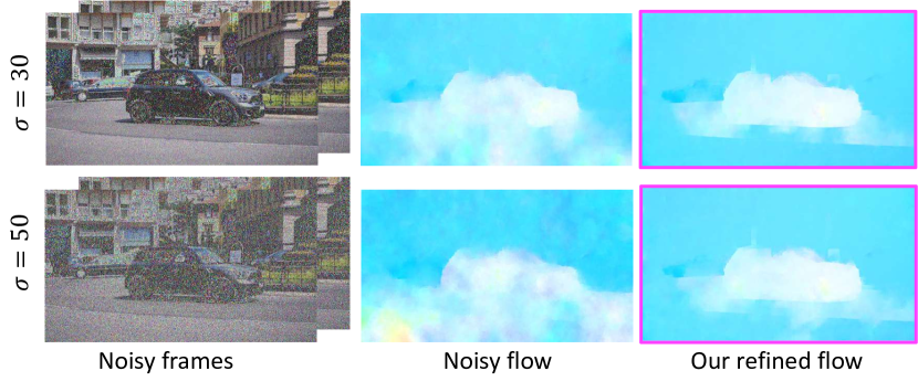
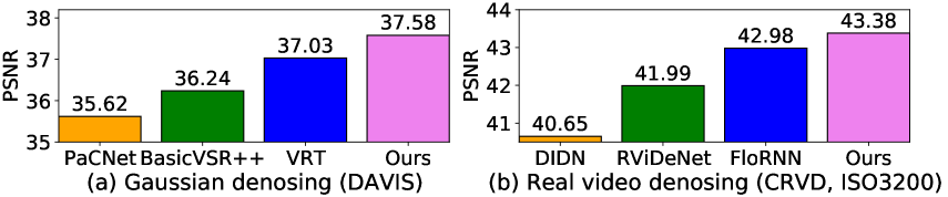
Figure 1: Effect of Noise on flow (above) and comparisons with previous SOTA on both synthesized and real denoising (blow). Our method outperforms all methods with a large margin.

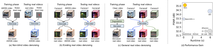
Figure 2: Discussion on the difference of existing video denoising setups. (a) Non-blind denoising methods take an AWGN video and its noise as input to synthesize a clean video. (b) Existing real denoising methods aim to map a noisy video to a clean video without inputting the noise level. When training a model with noisy videos from a specific camera, it has poor performance (marked by the dotted line) on another camera. (c) We first synthesizes different kinds of noisy videos with the degradation models, and then generalize well on different real-world videos. (d) Our method outperforms existing state-of-the-art video denoising methods and maintains good efficiency.

To address these, we design a new architecture to better exploit the flow guidance for video denoising. The new architecture progressively introduces and refines more flow information from low resolution to high resolution. Our network consists of multiple scales, each of which has a denoising-oriented flow refinement (DFR) module and a flow-guided mutual denoising propagation (FMDP) module. Without directly using off-the-shelf flows, DFR optimizes the flow estimation networks by minimizing the loss between the noisy flows and clean flows. In this way, DFR is able to reduce the sensitivity of the flow estimation networks to different levels of noise. The FMDP module uses the refined flows to mutually guide the forward and backward propagation in each scale. Based on the refined flows, this module learn diverse offsets to discover more meaningful and relevant features.

The contributions can be summarized as follows:

• We design a simple-but-effective video denoising architecture. Our proposed method achieves the state-of-the-art performance on both additive white Gaussian denoising tasks and real-world video denoising tasks. Moreover, our model achieves faster runtime than Transformer-based methods.

• We propose a denoising-oriented flow refinement (DFR) module and enables the flow estimation networks to be robust to different noise levels. Based on the refined flows, we also propose a flow-guided mutual denoising propagation (FMDP) module in which more meaningful and relevant texture can be exploited and they can be mutually propagated and aligned in different scales.

• We propose a new real video degradation model by simulating the real-world noise. The synthesized noisy videos can cover well a large range of real-world distribution. In addition, we collect a new real-world noisy videos dataset comprising diverse real-world noises. Our dataset can be utilized as a benchmark for evaluating the performance of real video denoising methods.

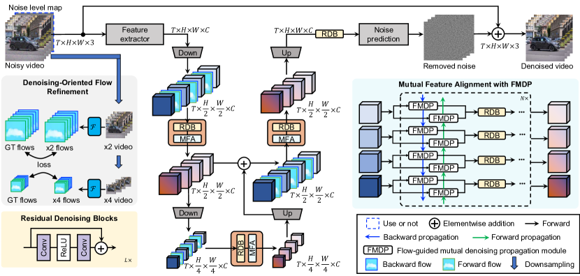
Figure 3: The architecture of the proposed multi-scale recurrent network. Our network is motivated by video noise properties. For non-blind video denoising, we take the noisy video and noise level map as an input. For real video denoising, we feed the noisy video augmented by our degradation models to train the network. At each scale, we use the denoising-oriented flow refinement (DFR) module to optimize flows and then use the flow-guided mutual denoising propagation (FMDP) to mutually guide the forward and backward propagation.

2 Related Work

Image denoising aims to reduce noise from a noisy image [30, 21, 41, 3]. Early methods [16, 33] depend on specific priors and hand-tuned parameters in the optimization. To address this, recent methods exploit the benefits of DNNs [78, 54, 79] and Transformer [38, 37, 76]. In addition, many image denoising models [49, 4] train on real image pairs captured by one camera. However, these methods often have poor performance on other cameras. More recently, denoising methods aim to approach the real-world denoising problem by using more realistic noisy images in training. This is achieved by making use of datasets with real-noisy (or approximately real noisy) images [1, 31], by using camera pipelines to synthesize real noisy images [26, 5, 74, 15], or using generative methods to model the real noises [12, 29, 72, 9, 61, 25, 44]. Some methods use self-supervised training on clean real images without explicitly modeling real noises [65, 80, 30, 66, 24, 50]. While image based denoising methods can in theory be used for videos by treating each frame as a separate image, directly doing so ignores the fruitful temporal connections between different frames in a video.

Video denoising aims at removing noise to synthesize clean videos. Based on BM3D [16], VBM4D [42] presents a video filtering algorithm to exploit temporal and spatial redundancy of a video. Early works [13] use recurrent networks to capture sequential information. Recently, BasicVSR++ [6] improves the second-order grid propagation and flow-guided deformable alignment in RNN and extends video super-resolution to the video denoising [8]. In addition, some denoising methods adopt an asymmetric loss function [62] to optimize the networks, or propose patch-based video denoising algorithm [2, 17] to exploit the correlations among patches. PaCNet [59] combines a patch-based framework with CNN by augmenting video sequences with patch-craft frames. To further improve over patch-based methods, DVDnet [56] proposes spatial and temporal denoising blocks and trains them separately. To boost the efficiency, FastDVDnet [57] extends DVDnet [56] by using two denoising steps which composed of a modified multi-scale U-Net [53]. A few works also propose to improve performance with unknown noises by using self-supervised learning [55, 18, 19]. Recently, ViDeNN [14] proposes a blind denoising method trained either on AWGN noise or on collected real-world videos. VRT [36] proposes a video restoration transformer with parallel frame prediction, and achieves the state-of-the-art performance in video denoising. Existing optical-flow-based methods [63, 36, 35, 6, 69] mostly did not consider the impact of noises on the flow estimation. However, it is known that most flow estimation networks tend to deteriorate under noise [67]. This can lead to wrong feature alignment. Although TOFlow [67] learns the task-oriented flow, it neglects to further refine and exploit more compensation information when the flow is still not precise. To complete the discussion on existing video denoising works, we summarize the different setups in Figure 2.

3 Proposed Method

In this paper, we aim to design a new architecture for synthesized Gaussian denoising and real video denoising to synthesize a clean video from a noisy video sequence $\{{\bm{I}}_{1},\ldots,{\bm{I}}_{T}\}$. The proposed architecture is provided in Figure 3. Our proposed architecture is multi-scale and it contains a down-scaling and a up-scaling processing. At each scale, the model has a denoising-oriented flow refinement and mutual feature alignment (MFA) with the flow-guided denoising propagation. First, we use an encoder to extract low-level features of a given noisy video sequence. On the other hand, we propose to refine the optical flows between local noisy neighbors at each scale. Second, we use the refined optical flows guilds the module for better feature alignment and propagation. Last, we further remove the spatial noise in the up-scaling. Note that all modules are differentiable and can be train in an end-to-end manner.

3.1 Denoising-Oriented Flow Refinement

The noise in each frame can be regarded as pixel occlusion. Different levels of noise produce different occlusions which thus affect the quality of the estimated optical flow, especially for strong noise as shown in Figure 1. Under the high level of noise, using an inaccurate optical flow may lead to misleading feature alignment and propagation. To address this, we propose a denoising-oriented flow refinement.

Without using the optical flow of the original size, we calculate the optical flows of the down-scaling frames. Specifically, we first downscale the noisy frames as ${\bm{I}}^{\downarrow s}$ using a bicubic operation at $\frac{1}{s}$ resolution. Then, the optical flow between adjacent downsampled frames ${\bm{I}}^{\downarrow s}_{i}$ and ${\bm{I}}^{\downarrow s}_{j}$ can be computed by a flow estimation network $F$, i.e.

$$\hat{{\bm{o}}}_{i{\to}j}^{s}={\mathcal{F}}\left({\bm{I}}^{\downarrow s}_{i},{\bm{I}}^{\downarrow s}_{j}\right),$$ (1)

where $\downarrow_{s}$ is downsampling with the scale $s$, and ${\mathcal{F}}$ is a flow estimation network.

A video contains a long-range of temporal information. To exploit such information, the forward and backward optical flows are important for feature propagation [6]. To this end, we propose to minimize the following $\ell_{1}$ loss to refine the optical flows, i.e.

$${\mathcal{L}}_{\text{flow}}=\sum\nolimits_{s,t}\left\|\hat{{\bm{o}}}_{t{\to}t+\Delta t}^{s}-{{\bm{o}}}_{t{\to}t+\Delta t}^{s}\right\|_{1},$$ (2)

where the scale $s{\in}\{2,4\}$, the neighbor $\Delta t{\in}\{{\pm}1\}$, and ${{\bm{o}}}_{t{\to}t+\Delta t}^{s}$ are the pseudo ground-truth forward or backward flows of noise-free clean videos. Specifically, the flow network ${\mathcal{F}}_{fixed}$ used to calculate ${{\bm{o}}}_{t{\to}t+\Delta t}^{s}$ is fixed. The flow network ${\mathcal{F}}$ used to calculate $\hat{{\bm{o}}}_{t{\to}t+\Delta t}^{s}$ is learnable. In our experiment, both networks use the same architecture and are initialized by the pre-trained weights of SpyNet [51]. In the experiment, we train the flow estimation network in an end-to-end manner. In this way, the optical flows are denoising-oriented and robust to different levels of noise.

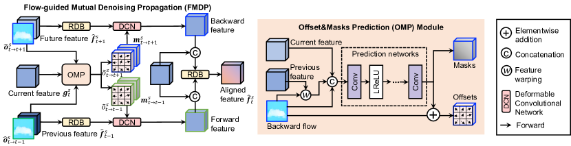
Figure 4: The architecture of the flow-guided denoising mutual-propagation. Given previous and future features, refined optical flows, and current features, we first estimate the offsets and masks in DCN, and then we obtain the backward and forward features. Last, we fuse these features with a convolution to obtain the final aligned features.

3.2 Flow-guided Mutual Denoising Propagation

With the help of our denoising-oriented flow refinement, optical flows contain temporal information which is important for feature alignment and propagation. Therefore, we propose a flow-guided denoising propagation module. Specifically, given an $T$-frame noisy video $\{{\bm{I}}_{1},\ldots,{\bm{I}}_{T}\}$, we first deploy a convolutional layer as the feature extractor to learn low-level features $\{\widehat{{\bm{g}}}_{1},\ldots,\widehat{{\bm{g}}}_{n}\}$. Then we use the residual block to extract deep features ${\bm{g}}_{t}^{s}$ and reduce the noise at the $i$-th time step of the $s$-scale. On the other hand, we use our denoising-oriented flow network to estimate the forward flows $\hat{{\bm{o}}}_{t{\to}t{-}1}$ and backward flows $\hat{{\bm{o}}}_{t{\to}t{+}1}$. Last, based on the denoising features ${\bm{g}}_{i}^{s}$, neighboring features ${\bm{f}}_{t{-}1}^{s}$ and ${\bm{f}}_{t{+}1}^{s}$ and the refined flows, we are able to mutually guide the denoising propagation to learn the denoising features $\hat{{\bm{f}}}_{t}^{s}$ at the current time step of the $s$-scale. Formally, we define a flow-guided denoising propagation as:

$$\!\!\!\hat{{\bm{f}}}_{t}^{s}{=}{\mathcal{A}}\left({\mathcal{P}}_{f}({\bm{g}}_{t}^{s},{\bm{f}}_{t{-}1}^{s},\hat{{\bm{o}}}_{t{\to}t{-}1}),{\mathcal{P}}_{b}({\bm{g}}_{t}^{s},{\bm{f}}_{t{+}1}^{s},\hat{{\bm{o}}}_{t{\to}t{+}1})\right)\!\!,\!\!\!\!$$ (3)

where ${\mathcal{A}}$ is an aggregation function which is implemented as a $1{\times}1$ convolutional layer in the expriment, ${\mathcal{P}}_{f}$ is the forward propagation function and ${\mathcal{P}}_{b}$ is the backward propagation function. Our mutual propagation module is able to jointly propagate forward and backward features in the next propagation, which is different from BasicVSR++ [6] which use backward and forward propagation in order in one scale. In contrast, our forward and backward propagation are processed in multiple scales which can aggregate more information for denoising.

Next, we will model the procedure of the forward propagation, and the procedure of the backward propagation can be formulated similarly but in the opposite direction. Given the denoising features ${\bm{g}}_{i}^{s}$, neighboring features ${\bm{f}}_{t{-}1}^{s}$ and the refined flows $\hat{{\bm{o}}}_{t{\to}t{-}1}$, we define the forward propagation as:

$${\mathcal{P}}_{f}({\bm{g}}_{t}^{s},{\bm{f}}_{t{-}1}^{s},\hat{{\bm{o}}}_{t{\to}t{-}1})={\mathcal{R}}\left({\bm{g}}_{t}^{s},{\mathcal{T}}({\bm{f}}_{t{-}1}^{s},\hat{{\bm{o}}}_{t{\to}t{-}1})\right),$$ (4)

where ${\mathcal{R}}$ consists of multiple residual layers, i.e. RDB, and ${\mathcal{T}}$ is the spatial texture transfer function according to the optical flows, which can be defined as:

$${\mathcal{T}}({\bm{f}}_{t{-}1}^{s},\hat{{\bm{o}}}_{t{\to}t{-}1})={\mathcal{D}}({\bm{f}}_{t{-}1}^{s},\widetilde{{\bm{o}}}^{s}_{t\rightarrow t{-}1},{\bm{m}}^{s}_{t\rightarrow t{-}1}),$$ (5)

where ${\mathcal{D}}$ is a deformable convolutional network (DCN) [82], $\widetilde{{\bm{o}}}^{s}_{t\rightarrow t{-}1}$ and ${\bm{m}}^{s}_{i\rightarrow i-p}$ are the offsets and masks. The relationship between our refined optical flows and the learned offsets can promote each other. The refined optical flows initialize the meaningful sampling locations and use the these flows to learn a set of offsets. These offsets have large diversity and provide more flexible locations for sampling in DCN. These sampling locations allow the model to discover more meaningful relevant texture in a local region and reduce warping error. As a result, these diverse offsets relieve the effects of the noise occlusion. On the other hand, these learned offsets provide positive feedback to further update the optical flows. The offsets and masks are formulated as

$$\widetilde{{\bm{o}}}^{s}_{t\rightarrow t-1} =\hat{{\bm{o}}}^{s}_{t\rightarrow t-1}+c_{1}\left(\left[{\bm{g}}_{t}^{s};\bar{{\bm{f}}}_{t-1}^{s};\hat{{\bm{o}}}^{s}_{t\rightarrow t-1}\right]\right),$$ (6)

$${\bm{m}}^{s}_{i\rightarrow t-1} =\tau(c_{2}\left(\left[{\bm{g}}_{t}^{s};\bar{{\bm{f}}}_{t-1}^{s};\hat{{\bm{o}}}^{s}_{t\rightarrow t-1}\right]\right)),$$ (7)

where $\tau$ is a Sigmoid function, $[\cdot;\cdot]$ is a concatenation operation, $c_{1}$ and $c_{2}$ are convolutional layers, and ${\bm{f}}_{t-1}^{s}$ is a warped feature using the optical flow $\hat{{\bm{o}}}^{s}_{t\rightarrow t-1}$, i.e.

$$\bar{{\bm{f}}}_{t-1}^{s}=\omega({\bm{f}}_{t-1}^{s},\hat{{\bm{o}}}^{s}_{t\rightarrow t-1}),$$ (8)

where $\omega(\cdot)$ is a warp function according to the optical flow. Based on the above formulations, we obtain the propagation features in each scale. At the last scale, we apply RDB blocks and a convolution layer as the noise prediction to learn the final residual and use the skip connection to obtain the denoised videos.

In this prorogation module, we do not directly use the second-order flows since the noise affects the accuracy of computation of flows and such error will be accumulated in the next propagation when the first-order optical flow is inaccurate, as shown in the supplementary. Our method can be extended to use second-order flows which can be our flow refinement module to reduce the propagation error.

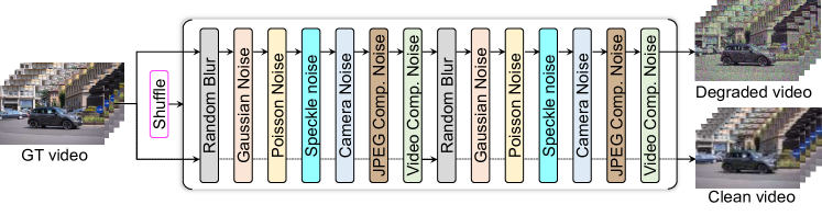
Figure 5: An illustration of the proposed noise degradation pipeline. For a high-quality video, a randomly shuffled degradation sequence is performed to produce a noisy video. The dash line means that we do not pass a certain degradation.

3.3 Real Noise Degradations

Real noise distribution is different from Gaussian noise, which is purely additive and signal-dependent. Training on Gaussian noise may have poor performance on real noise distribution. Real-world videos often contain unknown noises and blur, and they differ from video to video. To cover the real noise distribution, we propose to a large range of noise, including signal dependent and independent noise. Formally, given a GT video ${\bm{I}}_{{HR}}$, we use the following shuffled degradation process to synthesize a noisy and a clean video:

$$({\bm{I}},{\bm{I}}_{{clean}})=\left(g_{i_{1}}\circ g_{i_{2}}\circ\cdots\circ g_{i_{N}}\right)({\bm{I}}_{{HR}}),$$ (9)

where $\{i_{1},\ldots,i_{N}\}=\phi(\{1,\ldots,N\})$, $N$ is the number of degradations, $\phi$ is a shuffle function, $\circ$ is a function composition, and $g_{i_{n}}$ is a degradation model of the $i_{n}$-th type.

In practice, we propose use the following noise degradations, including Gaussian noise, Poisson noise, Speckle noise, Processed camera sensor noise, JPEG compression noise and video compression noise. We use Gaussian and Poisson noise because the noise in raw domain contains the read noise and shot noise which can be modeled by Gaussian and Poisson noise [20, 45]. Speckle noise exists in the synthetic aperture radar (SAR), medical ultrasound and optical coherence tomography images. Besides, we also consider processed camera sensor noise which originates from the image signal processing (ISP). Inspired by [76], the reverse ISP pipeline first get the raw image from an RGB image, then the forward pipeline constructs noisy raw image by adding noise to the raw image. For the digital images storage problem, JPEG compression noise and video compression noise are very important. Existing noise degradation models ignore the video compression noise, which are different from our model. More details of above degradations are put in the supplementary materials.

Apart from noise, most real videos inherently suffer from blurriness. Thus, we additionally consider two common blur degradations, i.e. Gaussian blur and resizing blur. As suggested in [76], we apply the same blur degradations on both noisy video and its clean counterpart, which is very different from existing super-resolution degradation models [77, 64]. The reason is that blur degradations will change the resolution of latent clean videos of the noisy videos.

Table 1: Quantitative comparison (average RGB channel PSNR/SSIM) with state-of-the-art methods for video denoising on the DAVIS and Set8 datasets. The best results are in bold.

Datasets	$\sigma$	VBM4D [42]	VNLB [2]	DVDnet [56]	FastDVDnet [57]	VNLNet [17]	PaCNet [58]	BasicVSR++ [8]	VRT [36]	Ours
DAVIS [28]	10	37.58/-	38.85/-	38.13/.9657	38.71/.9672	39.56/.9707	39.97/.9713	40.13/.9754	40.82/.9776	41.11/.9797
	20	33.88/-	35.68/-	35.70/.9422	35.77/.9405	36.53/.9464	37.10/.9470	37.41/.9598	38.15/.9625	38.61/.9677
	30	31.65/-	33.73/-	34.08/.9188	34.04/.9167	-/-	35.07/.9211	35.74/.9456	36.52/.9483	37.10/.9569
	40	30.05/-	32.32/-	32.86/.8962	32.82/.8949	33.32/.8996	33.57/.8969	34.49/.9319	35.32/.9345	35.98/.9465
	50	28.80/-	31.13/-	31.85/.8745	31.86/.8747	-/-	32.39/.8743	33.45/.9179	34.36/.9211	35.08/.9363
	​​Avg.​​	32.39/-	34.34/-	34.52/.9195	34.64/.9188	-/-	35.62/.9221	36.24/.9461	37.03/.9488	37.58/.9574
Set8 [56]	10	36.05/-	37.26/-	36.08/.9510	36.44/.9540	37.28/.9606	37.06/.9590	36.83/.9574	37.88/.9630	38.07/.9661
	20	32.18/-	33.72/-	33.49/.9182	33.43/.9196	34.02/.9273	33.94/.9247	34.15/.9319	35.02/.9373	35.41/.9456
	30	30.00/-	31.74/-	31.68/.8862	31.68/.8889	-/-	32.05/.8921	32.57/.9095	33.35/.9141	33.87/.9272
	40	28.48/-	30.39/-	30.46/.8564	30.46/.8608	30.72/.8622	30.70/.8623	31.42/.8889	32.15/.8928	32.76/.9101
	50	27.33/-	29.24/-	29.53/.8289	29.53/.8351	-/-	29.66/.8349	30.49/.8690	31.22/.8733	31.88/.8942
	​​Avg.​​	30.81/-	32.47/-	32.29/.8881	32.31/.8917	-/-	32.68/.8946	33.09/.9113	33.92/.9160	34.40/.9286

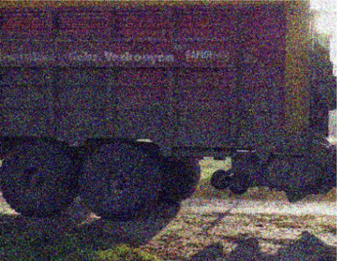
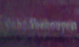
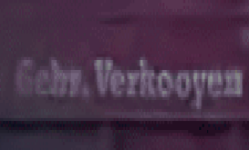
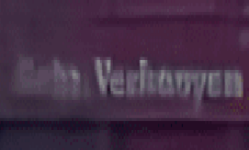
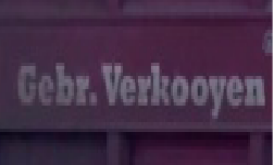
00000019, tractor, DAVIS [28] Noisy frame ($\sigma{=}50$) VBM4D [42] DVDnet [56] FastDVDnet [57] BasicVSR++ [6] VRT [36] Ours GT

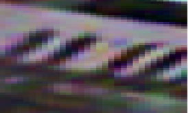
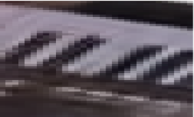
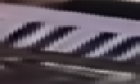
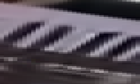
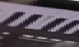
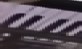
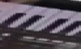
00000042, cats-car, DAVIS [28] Noisy frame ($\sigma{=}50$) VBM4D [42] DVDnet [56] FastDVDnet [57] BasicVSR++ [6] VRT [36] Ours GT

Figure 6: Visual comparison of different methods on DAVIS under the noise level of 50. More results are in Supplementary.

4 Experiments

4.1 Synthetic Gaussian Denoising

Datasets. We use DAVIS [28] and Set8 [56] in our synthetic Gaussian denoising experiments. We train all models on DAVIS training set [28], and test them on DAVIS testing set and Set8 [56]. Specifically, DAVIS [28] contains 90 training sequences (6208 frames) at 480p resolution, and 30 testing sequences (2086 frames) of resolution 854${\times}$480. Set8 [56] has 8 testing video sequences with a resolution of 960${\times}$540. Following the setting of [36], we synthesize the noisy video sequences by adding AWGN with noise level $\sigma{\in}[0,50]$ on the DAVIS [28] training set. We then train the model by using the synthesized data and test it on the DAVIS testing set and Set8 [56] with different Gaussian noise levels $\{10,20,30,40,50\}$. We compare our model with the following state-of-the-art video denoising methods, including VBM4D [42], VNLB [2], DVDnet [56], FastDVDnet [57], VNLNet [17], PaCNet [58], BasicVSR++ [8], and VRT [36].

Quantitative comparison. In Table 1, we show PSNR and SSIM of different methods on the DAVIS testing set [28] and Set8 [56] under different noise levels. Compared with other methods, our method has the best performance on both DAVIS and Set8 with a large margin. Specifically, our model outperforms BasicVSR++ [8] and previous SOTA VRT [36] by an average PSNR of 1.34dB and 0.55dB, respectively. These methods are influenced by noise since they neglect to learn robust flow networks. Moreover, the improvement of our method increases as the noise levels increase with the help of denoising-oriented pyramid flows. These results demonstrate the superiority of our proposed architecture.

Qualitative comparison. In Figure 6, we compare different methods under the high noise level of 50. Our proposed denoiser restores better structures and preserves clean edge than previous state-of-the-art video denoising methods, even though the noise level is high. In particular, our model is able to restore the letters ‘Gebr’ in the first example and piano texture in the second example of Figure 6. In contrast, VBM4D [42], DVDnet [56] and FastDVDnet [57] fail to remove severe noise from a video frame. BasicVSR++ [6] and VRT [36] only restore part of the textures.

Table 2: Quantitative comparison (average RGB channel PSNR) with state-of-the-art methods for video denoising on the CRVD (indoor) datasets [70]. The best results are in bold. The superscript ^∗ indicates the results are from the paper of RViDeNet [71].

ISO	ViDeNN∗ [14]	VBM4D∗ [42]	TOFlow∗ [67]	SMD∗ [11]	EDVR∗ [63]	DIDN∗ [68]	RViDeNet∗ [71]	FloRNN [35]	Ours
1600	35.44/0.966	39.34/0.967	37.61/0.964	37.81/0.969	42.10/0.984	41.85/0.985	43.13/0.988	44.07/0.991	44.10/0.992
3200	34.37/0.946	36.62/0.951	36.97/0.958	37.07/0.964	41.03/0.980	40.65/0.980	41.99/0.985	42.98/0.988	43.38/0.990
6400	31.87/0.880	33.75/0.925	35.42/0.940	35.93/0.958	38.98/0.974	38.82/0.975	39.99/0.980	41.04/0.985	41.15/0.986
12800	29.79/0.778	31.59/0.902	33.54/0.910	34.91/0.952	37.47/0.967	37.54/0.970	38.44/0.975	39.64/0.981	39.89/0.982
25600	25.95/0.559	29.48/0.868	30.52/0.835	33.64/0.942	35.26/0.957	35.28/0.960	36.21/0.968	37.34/0.976	37.56/0.979
Avg.	34.16/0.922	34.81/0.921	34.81/0.921	35.87/0.957	38.97/0.972	38.83/0.974	39.95/0.979	41.01/0.984	41.22/0.986

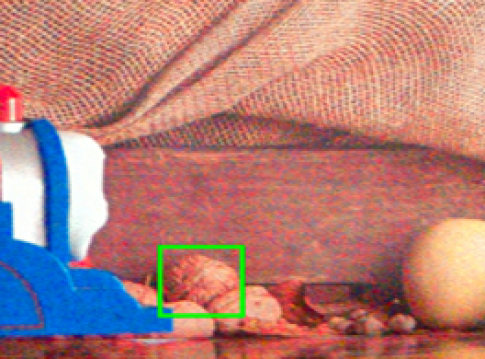
scene10, ISO25600, frame4 Noisy frame (26.83dB) ViDeNN [14] (28.25dB) TOFlow [67] (31.76dB) SMD [11] (31.31dB) DIDN [68] (33.82dB) RViDeNet [71] (35.88dB) Ours (36.90dB) GT (PSNR)

Figure 7: Visual comparison and PSNR (dB) of different methods on CRVD indoor dataset [70].

4.2 Real-world Video Denoising

4.2.1 Results on the CRVD Dataset

The CRVD dataset [70] is captured in the raw domain and it contains 6 indoor scenes for training and 5 indoor scenes for testing. Besides, it has 10 dynamic outdoor scenes without ground-truth clean videos. For each scene, the dataset has 5 different ISO settings. To evaluate our model on this dataset, we first apply a trained ISP model to raw data to generate sRGB videos, then we train our model on 6 indoor scenes.

In Table 2, we mainly compare raw video denoising methods in the sRGB domain under different ISO settings. Our method has the highest PSNR and SSIM across all ISO settings and thus achieves the best performance. In Figure 7, our method has higher PSRN with more high-frequency details and less noise. In contrast, ViDeNN [14] and TOFlow [67] still retain most of the noise in the video frames. Other methods remove the high-frequency texture when denoising. In addition, because the CRVD outdoor videos do not have ground-truth clean videos, we compare the visual results of different methods in the supplementary materials.

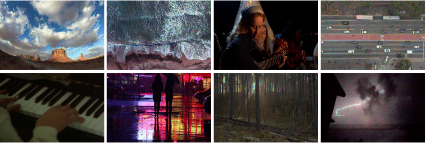
Figure 8: Our NoisyVideo consists of videos with a wide range of content and different types of unknown noise. It can be served as a common ground for future comparison of real video denoising.

Table 3: Quantitative Comparison of different methods on our RealNoise dataset for the real video denoising task.

Methods	NIQE$\downarrow$	BRISQUE$\downarrow$	PIQE$\downarrow$
VBM4D [42]	4.2692	43.4138	56.7153
Restormer [73]	3.7348	34.2775	47.8616
SCUNet [76]	3.3543	31.1964	42.3837
ViDeNN [14]	4.2911	21.9146	30.5148
FloRNN [35]	4.2568	33.4969	55.9694
BasicVSR++ [6]	3.7767	24.7670	29.3206
Ours-real	3.2818	21.7689	30.2147

4.2.2 Results on the Proposed RealNoise Video Dataset

To evaluate performance on more realistic videos, we additionally propose a new benchmark test dataset for real-world video denoising, called RealNoise. This dataset is collected from Pexels, with videos under the Creative Common license. It contains of 10 diverse scene types with different unknown noises, and each video contains at least 100 frames with no scene change. Examples of the dataset are shown in Figure 8 and further details are provided in the supplementary.

For training of the real video denoising model, we use REDS [48] as the training set. To have a fair comparison with other methods, we follow the setting of [63], and use 266 regrouped training clips and 4 testing clips (denoted as REDS4), where each with 100 consecutive frames. During training, we synthesize noisy videos on the REDS training set by using our proposed noise degradation model.

As shown in Figure 9, the proposed method achchives better visual quality than other image restoration methods and camera-based denoising methods. Our method is able to synthesize sharper texture. In contrast, traditional method VBM4D [42] only remove the part of noise. Restormer [73] and SCUNet [76] are image denoising methods and have limited performance when the real noise is complex because they do not exploit the temporal information. ViDeNN [14] and FloRNN [35] introduce artifacts in the video since they are trained on a specific camera. In Table 3, we compare different methods on our dataset. Here, we use three non-reference metrics NIQE [47], BRISQUE [46] and PIQE [60] as evaluation metrics because they are commonly used to measure the quality of images and ground-truth videos are not available. Our method shows very competitive results in all three scores as well. Note that these metrics do not always match perceptual visual quality [40]. From the visual example, with the help of our noise degradation model, our denoiser is able to reduce real-world noise.

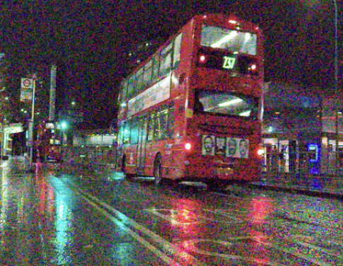
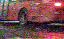
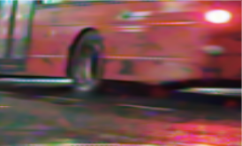
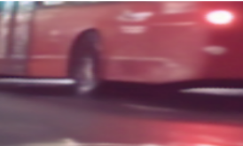
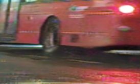
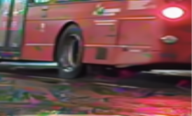
RealNoise, street, frame3 Noisy frame VBM4D [42] Restormer [73] SCUNet [76] ViDeNN [14] FloRNN [35] BasicVSR++ [8] Ours

Figure 9: Visual comparison of different methods on our proposed RealNoise dataset.

Table 4: Abaltion study on DAVIS [28] ($\sigma{=}50$).

Multiscale		✓	✓	✓	✓
FGDP			✓	✓	✓
MFA				✓	✓
Refine flow					✓
PSNR	33.46	34.40	34.67	34.90	35.08
SSIM	0.9179	0.9220	0.9233	0.9278	0.9363

Table 5: PSNR for Clipped Gaussian noise.

	Noise levels (DAVIS)
Methods	10	30	50
ViDeNN [14]	37.13	32.24	29.77
FastDVDnet [57] ​​	38.65	33.59	31.28
PaCNet [58]	39.96	34.66	32.00
Ours-blind	40.94	36.79	34.65
Ours	41.00	36.91	34.83

Table 6: PSNR for image denoising.

	Noise levels (Set8)
Methods	15	25	50
BM3D [16]	29.00	28.64	26.50
Restormer [73]	34.36	31.40	28.57
SwinIR [37]	34.87	32.37	29.19
SCUNet [76]	34.82	32.34	29.14
Ours	36.47	34.49	31.77

Table 7: Ablation study on noise types on synthesized REDS4.

Degradation types	PSNR	SSIM
w/o blur degradation	26.94	0.7783
w/o processed camera sensor noise	27.10	0.7799
w/o video compression noise	27.02	0.7791
w/ all degradations	27.46	0.7912

Table 8: Comparisons of PSNR with different learning paradigms.

Types	Methods	DAVIS ($\sigma{=}30$)	Set8 ($\sigma{=}30$)
Traditional	VBM4D [42]	31.65	30.00
Unsupervised learning	UDVD [55]	33.78	32.90
Self-supervised learning	MF2F [18]	33.91	31.84
Supervised learning	Ours	37.10	33.87

4.3 Ablation Studies

Effectiveness of each module. We investigate the effectiveness of each module in Table 6. Specifically, we conduct experiments by removing these modules. The model without these modules has a performance drop, which demonstrates the importance of each module. These results demonstrate the importance of our proposed flow refinement, multiscale architecture, mutual alignment and FGDP.

Ablation study on noise types. To investigate the effectiveness of the noise types, we remove one noise degradation and compare the performance on our synthesized REDS4 with fixed blur and noise degradations. Here, we mainly consider blur degradations, camera noises, and video compression noises which usually require temporal information for better denoising. From Table 8, training without any kind of noise leads to inferior performance, which demonstrates the dominant role.

Efficiency. In Figure 2 (d), we also compare the model size and runtime across different methods to evaluate the efficiency of networks. Our model achieves the best performance gains with a similar model size and runtime. In particular, for the largest noise level of 50, our model outperforms VRT [36] with smaller model size and faster inference time. Our model yields a PSNR improvement of 0.72dB.

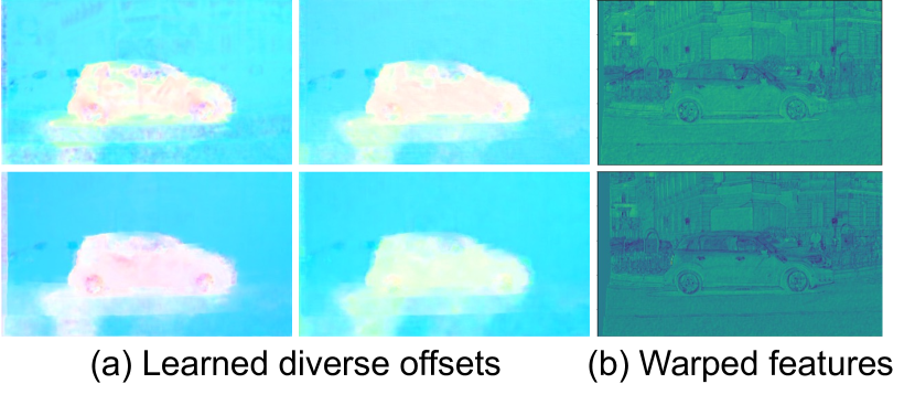
Figure 10: Results of flows, learned offsets and warped features.

Results of clipped noise image denoising. We also train non-blind and blind models on clipped AWGN of DAVIS. In Table 6, our model obtains the best performance under different noise levels. In addition, Table 6 shows that our method has better performance than image restoration methods since our model exploits the temporal information.

Diversity of learned offsets. We further visualize the diversity of the offsets and aligned features in Figure 10. With the refined flow and our proposed architecture, the diversity and quality of the offsets in the feature alignment can be increased. It means that the offset diversity helps the feature alignment to learn complementary offsets. In this way, it can alleviate the noise-occlusion issue and reduce warping errors. As a result, these offsets help yield better-warped features with more details during the feature propagation.

Different learning paradigms. We also compare our method with unsupervised learning and self-supervised learning paradigms (i.e. UDVD [55] and MF2F [18]) on DAVIS and Set8 datasets, as shown in Table 8. With the help of the ground-truth videos in the training, we are able to train a better model to map a noisy video to clean one.

Comparisons of flows. The optical flows between the frames ${\bm{I}}_{t}$ and ${\bm{I}}_{t+2}$ can be calculated directly or in a second-order way ( the same as [6]). We compare these two ways and show the visual quality of flows in the supplementary. The latter way causes the error will be accumulated in the propagation. In contrast, directly calculating the flow with our flow refinement has better performance.

Flow estimation robustness against noise. The proposed method leads to more robust flow estimation in the presence of different noise levels. More analysis is in the supplementary.

Video visual quality comparison. Quality of video denoising results can be better evaluated in the form of videos instead of images. In the supplementary, we provide more videos for comparison.

5 Conclusion

In this paper, we propose a simple-but-effective video denoising method which achieves state-of-the-art performance on both synthetic Gaussian denoising and real video denoising. Our proposed method mainly contains a denoising-oriented flow refinement (DFR) module and a flow-guided mutual denoising propagation (FMDP) module. The DFR module improves the robustness of the optical flow under different noise levels. The FMDP module makes use of the improved optical flow to mutually guide the feature propagation and alignment in multiple scales. Moreover, we design a new noise degradation model for the real-world video denoising task which considers different kinds of noise with a random shuffle. In addition, we propose a new real video denoising dataset with a large range of scenes and different noises. Our model has shown good generalization performance on unseen real videos. Extensive experiments demonstrate the effectiveness and superiority of our denoising method.

Organization.

In Section A, we provide detailed settings of our video noise degradations. In Section B, we provide more experimental details and additional results. It also includes the qualitative evaluation of the flow robustness against different noise levels (B.8). In Section B.9, we provide the flow comparison when trained in the first- or second-order fashion. In Section C, we discuss the limitations and societal impacts of our proposed method.

Appendix A Experiment Details of Noise Degradation

Noise. In the experiment, we consider 6 kinds of noises in the degradations, including Gaussian noise, Poisson noise, Speckle noise, Processed camera sensor noise, JPEG compression noise and video compression noise.

• Gaussian noise. When there is no prior information on noise, one can add Gaussian noise into a video sequence. Given a clean video ${\bm{I}}$, we synthesize a noisy video by

  $$g_{1}({\bm{I}})={\bm{I}}+{\bm{Z}},$$ (S1)

  where we sample the noise levels $\sigma$ in ${\bm{Z}}$ from $[2,50]$.

• Poisson noise. In electronics, Poisson noise is a type of shot noise that occurs in photon counting in optical devices. Such noise arises from the discrete nature of the electric charge, and it can be modeled by a Poisson process. Given a clean video ${\bm{I}}$, we synthesize a noisy video by

  $$g_{2}({\bm{I}})={\bm{I}}+{\bm{Z}},$$ (S2)

  where ${\bm{Z}}={\bm{Z}}^{\prime}-{\bm{I}}$ and ${\bm{Z}}^{\prime}\sim{\mathcal{P}}(10^{\alpha}\cdot{\bm{I}})/10^{\alpha}$. We add Poisson noise in color images by sampling different noise levels. We first multiply the clean video by $10^{\alpha}$ in the function of Poisson distribution, where ${\alpha}$ is uniformly chosen from $[2,4]$ and divide by $10^{\alpha}$.

• Speckle noise. Speckle noise exists in synthetic aperture radar (SAR), medical ultrasound and optical coherence tomography images. We simulate such noise by multiplying the clean image ${\bm{x}}$ and Gaussian noise ${\bm{Z}}$, i.e. ${\bm{I}}*{\bm{Z}}$. Then, we synthesize noisy video by

  $$g_{3}({\bm{I}})={\bm{I}}+{\bm{I}}*{\bm{Z}},$$ (S3)

  We sample the level of this noise from $[0,50]$.

• Processed camera sensor noise. In modern digital cameras, the processed camera sensor noise originates from image signal processing (ISP). Inspired by [76], the reverse ISP pipeline first gets the raw image from an RGB image, then the forward pipeline constructs a noisy raw image by adding noise to the raw image, which is denoted by

  $$g_{4}({\bm{I}})=\text{forward}(\text{reverse}({\bm{I}})).\vspace{-0.5cm}$$ (S4)

• JPEG compression noise. It is widely used to reduce the storage for digital images with fast encoding and decoding [77]. Such JPEG compression often causes $8\times 8$ blocking artifacts. The degree of blocking artifacts depends on the quality of compression. We synthesize frames by

  $$g_{5}({\bm{I}})=\text{Dec}(\text{Enc}({\bm{I}})).$$ (S5)

  The JPEG quality factor is uniformly chosen from $[30,95]$.

• Video compression noise. Videos sometimes have compression artifacts and are present on videos encoded in different formats. We use Pythonic av in FFmpeg, i.e.

  $$g_{6}({\bm{I}}){=}\text{av}({\bm{I}}).$$ (S6)

  We randomly selected codecs from [‘libx264’, ‘h264’, ‘mpeg4’] and bitrate from [1e4, 1e5] during training.

Blur. In addition to noise, most real-world videos inherently suffer from blurriness. Thus, we consider two blur degradations, including Gaussian blur and resizing blur.

• Gaussian blur. We synthesize Gaussian blur with different kernels, including [‘iso’, ‘aniso’, ‘generalized_iso’, ‘generalized_aniso’, ‘plateau_iso’, ‘plateau_aniso’, ‘sinc’]. We randomly choose these kernels with the probabilities of [0.405, 0.225, 0.108, 0.027, 0.108, 0.027, 0.1]. The settings of this blur are the same as [7].

• Resizing blur. We randomly draw the resize scales from [0.5, 2], and choose the interpolation mode from [‘bilinear’, ‘area’, ‘bicubic’] with the same probability of $1/3$.

Appendix B More Experiments

B.1 More Details of Experiment Setting

We adopt the Adam optimizer [32] and Cosine Annealing scheme [39] to decay the learning rate from $1{\times}10^{-4}$ to $10^{-7}$. The patch size is $256{\times}256$, and the batch size is 8. The number of input frames is 15. All experiments are implemented in PyTorch 1.9.1. We train the denoising model on 8 A100 GPUs. We use the pre-trained SPyNet [51] to estimate the flow and the SPyNet is further finetuned during training. We train our video denoiser with 150K iterations. For the synthetic Gaussian denoising experiments, the learning rate of the generator is $1{\times}10^{-4}$. For real-world video denoising, the learning rates of the generator and discriminator are set to $5{\times}10^{-5}$ and $1{\times}10^{-4}$. For the architecture of the generator, we use 5 residual blocks in the RDB block, use 7 residual blocks in the FMDP block, and set the feature channel as 64. The architectures of the offset estimation module and mask estimation module are the same as [6]. The architecture of the discriminator is the same as Real-ESRGAN [64]. When training classic video denoising, we use Charbonnier loss [10] because of its stability and good performance. For video denoising on AWGN noise and the CRVD indoor dataset, we use the loss ${\mathcal{L}}={\mathcal{L}}_{\text{pix}}+\lambda_{\text{flow}}{\mathcal{L}}_{\text{flow}}$. In the experiment, we set $\lambda_{\text{flow}}=0.1$. For real video denoising experiments, we first use Charbonnier loss to train a model, then we finetune the network by using the perceptual loss ${\mathcal{L}}_{\text{pix}}$ [27] and adversarial loss ${\mathcal{L}}_{\text{adv}}$ [22], i.e. ${\mathcal{L}}={\mathcal{L}}_{\text{pix}}+\lambda_{1}{\mathcal{L}}_{\text{per}}+\lambda_{2}{\mathcal{L}}_{\text{adv}}$, where $\lambda_{1}=1$ and $\lambda_{2}=5\times 10^{-1}$. Code will be made publicly available.

B.2 Training Loss and PSNR

To demonstrate the efficiency of our model, we show the training loss and PSNR validation, as shown in Figure S1. At every 10K iterations, the PSNR value is calculated on Set8 with the noise level of 10. The total training iterations is 150k and takes 3 days. The training loss decreases rapidly at early iterations and stays steady in the later iterations. The PSNR values on Set8 increase during the training. These results demonstrate that our model is easy to train to have good performance.

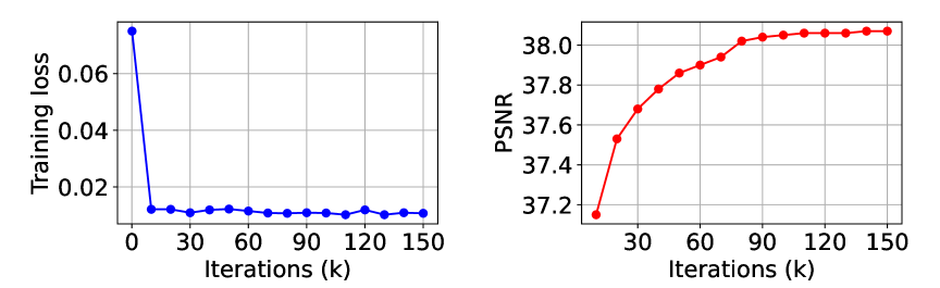
Figure S1: An illustration of training loss and PSNR.

B.3 Results on CRVD Outdoor Dataset

In Figure S2, we compare different methods under ISO25600. Our method has better visual quality than these methods. Specifically, our method synthesizes a sharper grid than other methods. Please zoom in for a better observation of the figure. In contrast, SMD [11], DIDN [68] and EDVR [63] have smooth textures and lose high-frequency details.

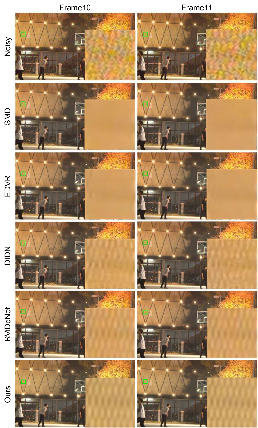
Figure S2: Visual comparisons of different methods for two consecutive frames from the outdoor scene4 under ISO25600. These visual results come from [71].

B.4 Comparison on FLOPs

Model inference time was provided in Figure 2 (d) in the paper, which can reflect the efficiency of the models. We compared the FLOPs and PSNR performance of different video denoising methods in Table S1. Here, the FLOPs is measured in TITAN RTX GPU with the spatial resolutions of $256{\times}256$. Our model achieves the best PSNR performance, although it has more FLOPs than BasicVSR++ [6] due to the multi-scales. Besides, our model outperforms VRT [36] with much fewer FLOPs.

Table S1: Comparison with different methods on FLOPs.

Methods	BasicVSR++ [6]	VRT [36]	Ours
FLOPs (G)	42.8	721.9	182.8
PSNR (dB)	36.24	37.03	37.58

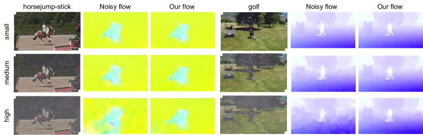
Figure S3: Visualization of flows for different levels of noise on DAVIS.

B.5 Generalization of Real Video Denoising Model

To investigate the generalization performance, we test our method on REDS4 testing set with different noise types. Specifically, we use REDS4 as a base and synthesize an additional noise type into the videos for each column in Table S2. The trained model is then tested on the synthesized video with new noise. The different noise types are Gaussian noise, Poisson noise, Speckle noise, Camera noise, JPEG compression noise and Video compression noise. The levels of Gaussian and Speckle noise are 10, the scale of Poisson is 0.05, the quality scale of JPEG compression noise is 80, and the codec and bitrate of Video compression noise are ‘mpeg4’ and $1e5$. Our video denoiser has good generalization performance on other noise.

Table S2: Generalization to different kinds of noise on REDS4.

Types	​​ Gaussian noise ​​	​​ Poisson noise ​​	​​ Speckle noise ​​	​​ Camera noise ​​	​​ JPEG comp. ​​	​​ Video comp. ​​
​​Ours-real​​	28.03	28.17	28.14	28.63	28.18	26.82

B.6 More Details of Our RealNoise Videos

To evaluate the generalization of real-world video denoising methods, it is important to collect a benchmark that covers a wide range of scenes and noises. Most existing datasets (e.g. [70]) are captured by one camera with different ISO settings. However, such a dataset has a distribution mismatching gap compared with real-world noisy videos. As a result, performing well in this kind of dataset may have poor generalization on videos in the wild. To address this, we propose to capture the RealNoise dataset and select as many scenes and noises as possible. For example, the collected noisy videos include low-light, underwater, aerial videos, old films, weather, people, street, forest and natural scenery etc. Due to the file size limits, we only provide small video examples with the denoising results in the supplementary. The full dataset will be released.

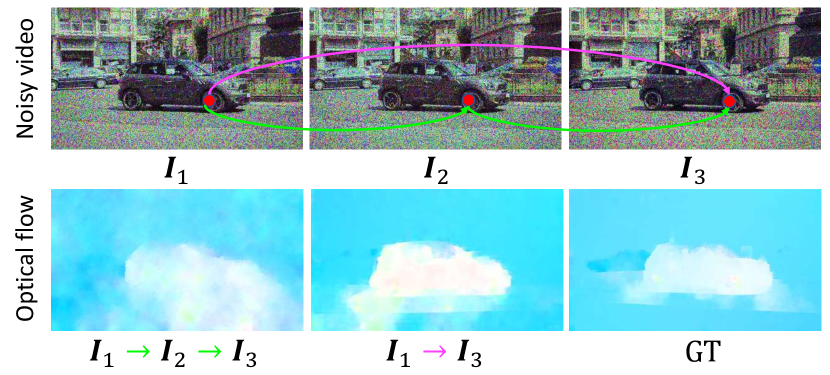
Figure S4: Cumulative effect of the error of second-order flows.

Table S3: Comparison with different types of flows.

Types	First-order	Second-order	Second-order with flow loss
PSNR	34.45	34.90	35.08

00000000, hypersmooth, Set8 Noisy frame ($\sigma{=}50$) VBM4D [42] DVDnet [56] FastDVDnet [57] BasicVSR++ [6] VRT [36] Ours GT

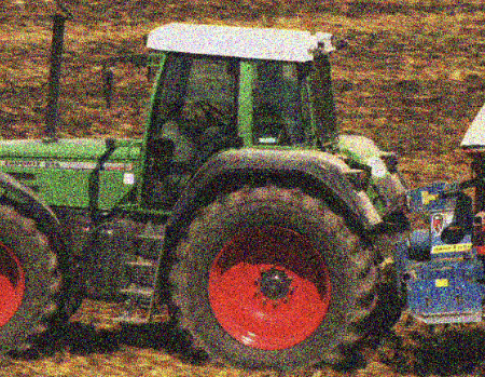
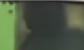
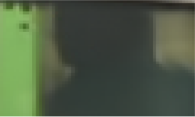
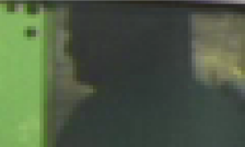
00000060, tractor, Set8 Noisy frame ($\sigma{=}50$) VBM4D [42] DVDnet [56] FastDVDnet [57] BasicVSR++ [6] VRT [36] Ours GT

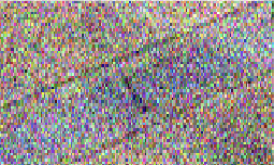
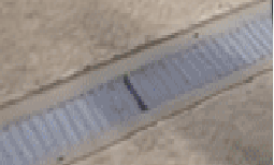
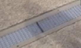
00000011, helicopter, DAVIS Noisy frame ($\sigma{=}50$) VBM4D [42] DVDnet [56] FastDVDnet [57] BasicVSR++ [6] VRT [36] Ours GT

00000073, golf, DAVIS Noisy frame ($\sigma{=}50$) VBM4D [42] DVDnet [56] FastDVDnet [57] BasicVSR++ [6] VRT [36] Ours GT

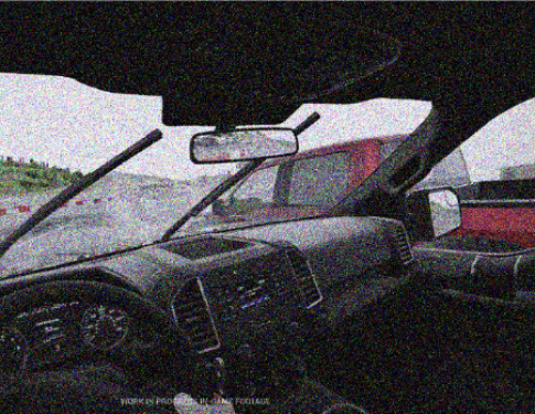
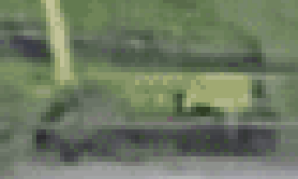
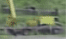
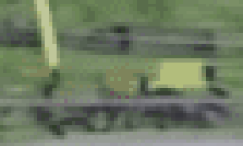
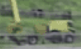
00000000, car-race, DAVIS Noisy frame ($\sigma{=}50$) VBM4D [42] DVDnet [56] FastDVDnet [57] BasicVSR++ [6] VRT [36] Ours GT

Figure S5: Visual comparison of different methods on DAVIS under the noise level of 50.

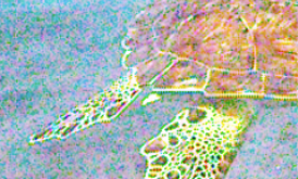
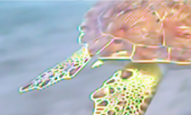
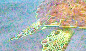
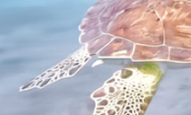
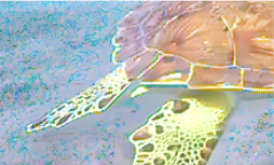
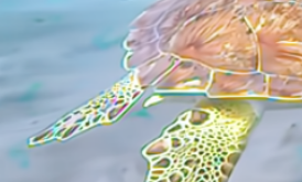
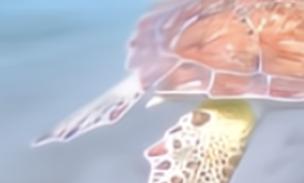
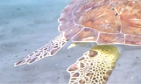
RealNoise, underwater, frame6 Noisy frame VBM4D [42] Restormer [73] SCUNet [76] ViDeNN [14] FloRNN [35] BasicVSR++ [8] Ours

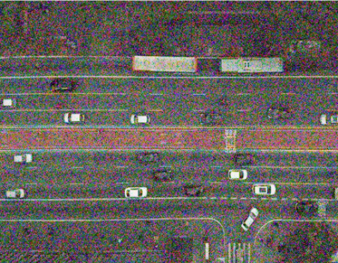
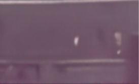
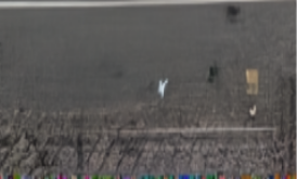
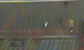
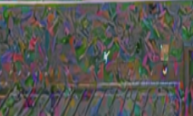
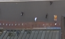
RealNoise, car, frame50 Noisy frame VBM4D [42] Restormer [73] SCUNet [76] ViDeNN [14] FloRNN [35] BasicVSR++ [8] Ours

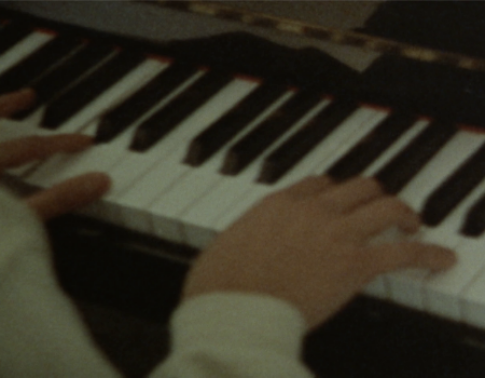
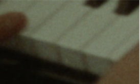
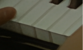
RealNoise, old_video, frame1 Noisy frame VBM4D [42] Restormer [73] SCUNet [76] ViDeNN [14] FloRNN [35] BasicVSR++ [8] Ours

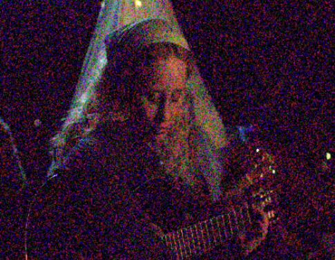
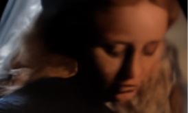
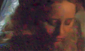
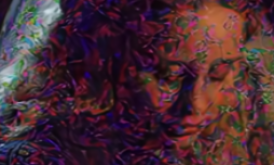
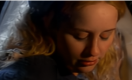
RealNoise, people, frame5 Noisy frame VBM4D [42] Restormer [73] SCUNet [76] ViDeNN [14] FloRNN [35] BasicVSR++ [8] Ours

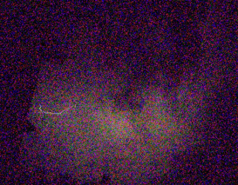
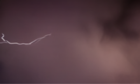
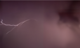
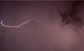
RealNoise, thunder, frame9 Noisy frame VBM4D [42] Restormer [73] SCUNet [76] ViDeNN [14] FloRNN [35] BasicVSR++ [8] Ours

Figure S6: Visual comparison of different methods on our proposed RealNoise dataset.

B.7 More Qualitative Comparison

In Figures S5 and S6, we provide more visual comparisons for synthetic Gaussian denoising and real video denoising on our NoisyVideo dataset. Our model restores better structures and preserves a cleaner edge than previous state-of-the-art video denoising methods, even though the noise level is high. In particular, our model is able to synthesize the side profile in the second line of Figure S5. For real video denoising, our model achieves the best visual quality among different methods. Specifically, our model can generate the stripe texture in the second example of Figure S6.

B.8 Flow Estimation Robustness Against Noise

To investigate the robustness of our model to different kinds and levels of noise, we visualize the estimated flows in Figure S3. We group the noise levels into small, medium and large by setting $\sigma{=}10,\sigma{=}30$ and $\sigma{=}50$, respectively. For the small and medium noise levels, the noisy flow and our flow have similar results. For the high noise level, our flow estimation model has a more robust performance. The proposed method leads to more robust flow estimation in the presence of different noise levels.

B.9 Comparisons with Flows

The optical flows between the frames ${\bm{I}}_{t}$ and ${\bm{I}}_{t+2}$ can be calculated directly or in a second-order way ( the same as [6]). We compare these two ways and show the visual quality of flows in Figure S4. The latter way causes the error will be accumulated in the propagation. In contrast, directly calculating the flow with our flow refinement has better performance.

In addition, we compare three settings as follows. (1) First-order flows mean that we estimate the optical flow of two adjacent frames, i.e. ${\bm{I}}_{t}{\to}{\bm{I}}_{t+1}$ and ${\bm{I}}_{t}{\to}{\bm{I}}_{t-1}$. (2) Second-order flows mean that we estimate the optical flow of two adjacent frames and two frames apart, i.e. ${\bm{I}}_{t}{\to}{\bm{I}}_{t+1},{\bm{I}}_{t}{\to}{\bm{I}}_{t-1},{\bm{I}}_{t}{\to}{\bm{I}}_{t+2}$ and ${\bm{I}}_{t}{\to}{\bm{I}}_{t-2}$. (3) We also compare the second-order flows optimized with our proposed flow loss. In Table S3, we compare these types of flows on DAVIS under $\sigma=50$. With the help of our flow refinement, using the second-order flows achieves the best performance.

Appendix C Limitations and Social Impacts

Our method achieves state-of-the-art performance in synthetic Gaussian denoising and real video denoising. This paper makes the first attempt to propose video noise degradations for real video denoising. Our method can be used in some applications with positive social impacts. For example, it can be used to restore old videos and remove compression noise from videos on the web. However, there are some limitations in practice. First, it is hard for our model to remove blur artifacts which often occur in videos due to exposure time in different cameras. However, our degradation pipeline mainly considers different kinds of noise. Second, it is challenging to remove big spot noise. Third, our denoiser is trained with the GAN loss and it may change the identity of details (e.g. human face) especially when the input is severely degraded.

References

- [1] Saeed Anwar and Nick Barnes. Real image denoising with feature attention. In IEEE International Conference on Computer Vision, pages 3155–3164, 2019.
- [2] Pablo Arias and Jean-Michel Morel. Video denoising via empirical bayesian estimation of space-time patches. Journal of Mathematical Imaging and Vision, 60(1), 2018.
- [3] Théo Bodrito, Alexandre Zouaoui, Jocelyn Chanussot, and Julien Mairal. A trainable spectral-spatial sparse coding model for hyperspectral image restoration. Advances in Neural Information Processing Systems, 2021.
- [4] Tim Brooks, Ben Mildenhall, Tianfan Xue, Jiawen Chen, Dillon Sharlet, and Jonathan T Barron. Unprocessing images for learned raw denoising. In IEEE Conference on Computer Vision and Pattern Recognition, 2019.
- [5] Yue Cao, Xiaohe Wu, Shuran Qi, Xiao Liu, Zhongqin Wu, and Wangmeng Zuo. Pseudo-isp: learning pseudo in-camera signal processing pipeline from a color image denoiser. arXiv preprint arXiv:2103.10234, 2021.
- [6] Kelvin CK Chan, Shangchen Zhou, Xiangyu Xu, and Chen Change Loy. Basicvsr++: Improving video super-resolution with enhanced propagation and alignment. In IEEE Conference on Computer Vision and Pattern Recognition, 2022.
- [7] Kelvin CK Chan, Shangchen Zhou, Xiangyu Xu, and Chen Change Loy. Investigating tradeoffs in real-world video super-resolution. In IEEE Conference on Computer Vision and Pattern Recognition, 2022.
- [8] Kelvin CK Chan, Shangchen Zhou, Xiangyu Xu, and Chen Change Loy. On the generalization of basicvsr++ to video deblurring and denoising. arXiv preprint arXiv:2204.05308, 2022.
- [9] Ke-Chi Chang, Ren Wang, Hung-Jin Lin, Yu-Lun Liu, Chia-Ping Chen, Yu-Lin Chang, and Hwann-Tzong Chen. Learning camera-aware noise models. In European Conference on Computer Vision, pages 343–358, 2020.
- [10] Pierre Charbonnier, Laure Blanc-Feraud, Gilles Aubert, and Michel Barlaud. Two deterministic half-quadratic regularization algorithms for computed imaging. In International Conference on Image Processing, 1994.
- [11] Chen Chen, Qifeng Chen, Minh N Do, and Vladlen Koltun. Seeing motion in the dark. In IEEE International Conference on Computer Vision, pages 3185–3194, 2019.
- [12] Jingwen Chen, Jiawei Chen, Hongyang Chao, and Ming Yang. Image blind denoising with generative adversarial network based noise modeling. In IEEE Conference on Computer Vision and Pattern Recognition, pages 3155–3164, 2018.
- [13] Xinyuan Chen, Li Song, and Xiaokang Yang. Deep rnns for video denoising. In Applications of Digital Image Processing XXXIX, 2016.
- [14] Michele Claus and Jan van Gemert. Videnn: Deep blind video denoising. In IEEE Conference on Computer Vision and Pattern Recognition Workshops, 2019.
- [15] Marcos V Conde, Steven McDonagh, Matteo Maggioni, Ales Leonardis, and Eduardo Pérez-Pellitero. Model-based image signal processors via learnable dictionaries. In Proceedings of the AAAI Conference on Artificial Intelligence, volume 36, pages 481–489, 2022.
- [16] Kostadin Dabov, Alessandro Foi, Vladimir Katkovnik, and Karen Egiazarian. Image denoising by sparse 3-d transform-domain collaborative filtering. IEEE Transactions on Image Processing, 2007.
- [17] Axel Davy, Thibaud Ehret, Jean-Michel Morel, Pablo Arias, and Gabriele Facciolo. Non-local video denoising by cnn. arXiv preprint arXiv:1811.12758, 2018.
- [18] Valéry Dewil, Jérémy Anger, Axel Davy, Thibaud Ehret, Gabriele Facciolo, and Pablo Arias. Self-supervised training for blind multi-frame video denoising. In IEEE Winter Conference on Applications of Computer Vision, pages 2724–2734, 2021.
- [19] Valéry Dewil, Arnaud Barral, Gabriele Facciolo, and Pablo Arias. Self-supervision versus synthetic datasets: which is the lesser evil in the context of video denoising? In IEEE Conference on Computer Vision and Pattern Recognition, pages 4900–4910, 2022.
- [20] Alessandro Foi, Mejdi Trimeche, Vladimir Katkovnik, and Karen Egiazarian. Practical poissonian-gaussian noise modeling and fitting for single-image raw-data. IEEE Transactions on Image Processing, 17(10):1737–1754, 2008.
- [21] Xueyang Fu, Zeyu Xiao, Gang Yang, Aiping Liu, Zhiwei Xiong, et al. Unfolding taylor’s approximations for image restoration. Advances in Neural Information Processing Systems, 2021.
- [22] Ian Goodfellow, Jean Pouget-Abadie, Mehdi Mirza, Bing Xu, David Warde-Farley, Sherjil Ozair, Aaron Courville, and Yoshua Bengio. Generative adversarial nets. Advances in neural information processing systems, 2014.
- [23] Cong Huang, Jiahao Li, Bin Li, Dong Liu, and Yan Lu. Neural compression-based feature learning for video restoration. In IEEE Conference on Computer Vision and Pattern Recognition, 2022.
- [24] Tao Huang, Songjiang Li, Xu Jia, Huchuan Lu, and Jianzhuang Liu. Neighbor2neighbor: Self-supervised denoising from single noisy images. In IEEE Conference on Computer Vision and Pattern Recognition, pages 14781–14790, 2021.
- [25] Geonwoon Jang, Wooseok Lee, Sanghyun Son, and Kyoung Mu Lee. C2n: Practical generative noise modeling for real-world denoising. In IEEE International Conference on Computer Vision, pages 2350–2359, 2021.
- [26] Ronnachai Jaroensri, Camille Biscarrat, Miika Aittala, and Frédo Durand. Generating training data for denoising real rgb images via camera pipeline simulation. arXiv preprint arXiv:1904.08825, 2019.
- [27] Justin Johnson, Alexandre Alahi, and Li Fei-Fei. Perceptual losses for real-time style transfer and super-resolution. In European conference on computer vision, 2016.
- [28] Anna Khoreva, Anna Rohrbach, and Bernt Schiele. Video object segmentation with language referring expressions. In Asian Conference on Computer Vision, 2018.
- [29] Dong-Wook Kim, Jae Ryun Chung, and Seung-Won Jung. Grdn: Grouped residual dense network for real image denoising and gan-based real-world noise modeling. In IEEE Conference on Computer Vision and Pattern Recognition Workshops, pages 0–0, 2019.
- [30] Kwanyoung Kim and Jong Chul Ye. Noise2score: tweedie’s approach to self-supervised image denoising without clean images. Advances in Neural Information Processing Systems, 34:864–874, 2021.
- [31] Yoonsik Kim, Jae Woong Soh, Gu Yong Park, and Nam Ik Cho. Transfer learning from synthetic to real-noise denoising with adaptive instance normalization. In IEEE Conference on Computer Vision and Pattern Recognition, pages 3482–3492, 2020.
- [32] Diederik P Kingma and Jimmy Ba. Adam: A method for stochastic optimization. In International Conference on Learning Representations, 2015.
- [33] Marc Lebrun, Antoni Buades, and Jean-Michel Morel. A nonlocal bayesian image denoising algorithm. SIAM Journal on Imaging Sciences, 2013.
- [34] Seunghwan Lee, Donghyeon Cho, Jiwon Kim, and Tae Hyun Kim. Restore from restored: Video restoration with pseudo clean video. In IEEE Conference on Computer Vision and Pattern Recognition, 2021.
- [35] Junyi Li, Xiaohe Wu, Zhenxing Niu, and Wangmeng Zuo. Unidirectional video denoising by mimicking backward recurrent modules with look-ahead forward ones. In European Conference on Computer Vision, pages 592–609, 2022.
- [36] Jingyun Liang, Jiezhang Cao, Yuchen Fan, Kai Zhang, Rakesh Ranjan, Yawei Li, Radu Timofte, and Luc Van Gool. Vrt: A video restoration transformer. arXiv preprint arXiv:2201.12288, 2022.
- [37] Jingyun Liang, Jiezhang Cao, Guolei Sun, Kai Zhang, Luc Van Gool, and Radu Timofte. Swinir: Image restoration using swin transformer. In IEEE International Conference on Computer Vision Workshops, 2021.
- [38] Ze Liu, Yutong Lin, Yue Cao, Han Hu, Yixuan Wei, Zheng Zhang, Stephen Lin, and Baining Guo. Swin transformer: Hierarchical vision transformer using shifted windows. In IEEE International Conference on Computer Vision, 2021.
- [39] Ilya Loshchilov and Frank Hutter. Sgdr: Stochastic gradient descent with warm restarts. arXiv preprint arXiv:1608.03983, 2016.
- [40] Andreas Lugmayr, Martin Danelljan, and Radu Timofte. Ntire 2020 challenge on real-world image super-resolution: Methods and results. In IEEE Conference on Computer Vision and Pattern Recognition Workshops, pages 494–495, 2020.
- [41] Fangzhou Luo, Xiaolin Wu, and Yanhui Guo. Functional neural networks for parametric image restoration problems. Advances in Neural Information Processing Systems, 2021.
- [42] Matteo Maggioni, Giacomo Boracchi, Alessandro Foi, and Karen Egiazarian. Video denoising, deblocking, and enhancement through separable 4-d nonlocal spatiotemporal transforms. IEEE Transactions on Image Processing, 2012.
- [43] Matteo Maggioni, Yibin Huang, Cheng Li, Shuai Xiao, Zhongqian Fu, and Fenglong Song. Efficient multi-stage video denoising with recurrent spatio-temporal fusion. In IEEE Conference on Computer Vision and Pattern Recognition, 2021.
- [44] Ali Maleky, Shayan Kousha, Michael S Brown, and Marcus A Brubaker. Noise2noiseflow: Realistic camera noise modeling without clean images. In IEEE Conference on Computer Vision and Pattern Recognition, pages 17632–17641, 2022.
- [45] Ben Mildenhall, Jonathan T Barron, Jiawen Chen, Dillon Sharlet, Ren Ng, and Robert Carroll. Burst denoising with kernel prediction networks. In IEEE Conference on Computer Vision and Pattern Recognition, pages 2502–2510, 2018.
- [46] Anish Mittal, Anush K Moorthy, and Alan C Bovik. Blind/referenceless image spatial quality evaluator. In Asilomar Conference on Signals, Systems and Computers, 2011.
- [47] Anish Mittal, Rajiv Soundararajan, and Alan C Bovik. Making a “completely blind” image quality analyzer. IEEE Signal Processing Letters, 2012.
- [48] Seungjun Nah, Sungyong Baik, Seokil Hong, Gyeongsik Moon, Sanghyun Son, Radu Timofte, and Kyoung Mu Lee. Ntire 2019 challenge on video deblurring and super-resolution: Dataset and study. In IEEE Conference on Computer Vision and Pattern Recognition Workshops, 2019.
- [49] Tobias Plotz and Stefan Roth. Benchmarking denoising algorithms with real photographs. In IEEE conference on computer vision and pattern recognition, 2017.
- [50] Yuhui Quan, Mingqin Chen, Tongyao Pang, and Hui Ji. Self2self with dropout: Learning self-supervised denoising from single image. In IEEE Conference on Computer Vision and Pattern Recognition, pages 1890–1898, 2020.
- [51] Anurag Ranjan and Michael J Black. Optical flow estimation using a spatial pyramid network. In IEEE conference on computer vision and pattern recognition, 2017.
- [52] Chao Ren, Xiaohai He, Chuncheng Wang, and Zhibo Zhao. Adaptive consistency prior based deep network for image denoising. In IEEE Conference on Computer Vision and Pattern Recognition, 2021.
- [53] Olaf Ronneberger, Philipp Fischer, and Thomas Brox. U-net: Convolutional networks for biomedical image segmentation. In International Conference on Medical image computing and computer-assisted intervention, 2015.
- [54] Venkataraman Santhanam, Vlad I Morariu, and Larry S Davis. Generalized deep image to image regression. In IEEE Conference on Computer Vision and Pattern Recognition, 2017.
- [55] Dev Yashpal Sheth, Sreyas Mohan, Joshua L Vincent, Ramon Manzorro, Peter A Crozier, Mitesh M Khapra, Eero P Simoncelli, and Carlos Fernandez-Granda. Unsupervised deep video denoising. In IEEE International Conference on Computer Vision, pages 1759–1768, 2021.
- [56] Matias Tassano, Julie Delon, and Thomas Veit. Dvdnet: A fast network for deep video denoising. In IEEE International Conference on Image Processing, 2019.
- [57] Matias Tassano, Julie Delon, and Thomas Veit. Fastdvdnet: Towards real-time deep video denoising without flow estimation. In IEEE Conference on Computer Vision and Pattern Recognition, 2020.
- [58] Gregory Vaksman, Michael Elad, and Peyman Milanfar. Patch craft: Video denoising by deep modeling and patch matching. In IEEE International Conference on Computer Vision, 2021.
- [59] Gregory Vaksman, Michael Elad, and Peyman Milanfar. Patch craft: Video denoising by deep modeling and patch matching. In IEEE International Conference on Computer Vision, 2021.
- [60] N Venkatanath, D Praneeth, Maruthi Chandrasekhar Bh, Sumohana S Channappayya, and Swarup S Medasani. Blind image quality evaluation using perception based features. In National Conference on Communications, 2015.
- [61] Duc My Vo, Duc Manh Nguyen, Thao Phuong Le, and Sang-Woong Lee. Hi-gan: A hierarchical generative adversarial network for blind denoising of real photographs. Information Sciences, 570:225–240, 2021.
- [62] Thijs Vogels, Fabrice Rousselle, Brian McWilliams, Gerhard Röthlin, Alex Harvill, David Adler, Mark Meyer, and Jan Novák. Denoising with kernel prediction and asymmetric loss functions. ACM Transactions on Graphics, 2018.
- [63] Xintao Wang, Kelvin CK Chan, Ke Yu, Chao Dong, and Chen Change Loy. Edvr: Video restoration with enhanced deformable convolutional networks. In IEEE Conference on Computer Vision and Pattern Recognition Workshops, 2019.
- [64] Xintao Wang, Liangbin Xie, Chao Dong, and Ying Shan. Real-esrgan: Training real-world blind super-resolution with pure synthetic data. In IEEE International Conference on Computer Vision, 2021.
- [65] Xiaohe Wu, Ming Liu, Yue Cao, Dongwei Ren, and Wangmeng Zuo. Unpaired learning of deep image denoising. In European Conference on Computer Vision, pages 352–368, 2020.
- [66] Yaochen Xie, Zhengyang Wang, and Shuiwang Ji. Noise2same: Optimizing a self-supervised bound for image denoising. Advances in Neural Information Processing Systems, 33:20320–20330, 2020.
- [67] Tianfan Xue, Baian Chen, Jiajun Wu, Donglai Wei, and William T Freeman. Video enhancement with task-oriented flow. International Journal of Computer Vision, 127:1106–1125, 2019.
- [68] Songhyun Yu, Bumjun Park, and Jechang Jeong. Deep iterative down-up cnn for image denoising. In IEEE Conference on Computer Vision and Pattern Recognition workshops, pages 0–0, 2019.
- [69] Songhyun Yu, Bumjun Park, Junwoo Park, and Jechang Jeong. Joint learning of blind video denoising and optical flow estimation. In IEEE Conference on Computer Vision and Pattern Recognition Workshops, pages 500–501, 2020.
- [70] Huanjing Yue, Cong Cao, Lei Liao, Ronghe Chu, and Jingyu Yang. Supervised raw video denoising with a benchmark dataset on dynamic scenes. In IEEE conference on computer vision and pattern recognition, pages 2301–2310, 2020.
- [71] Huanjing Yue, Cong Cao, Lei Liao, Ronghe Chu, and Jingyu Yang. Supervised raw video denoising with a benchmark dataset on dynamic scenes. In IEEE Conference on Computer Vision and Pattern Recognition, 2020.
- [72] Zongsheng Yue, Qian Zhao, Lei Zhang, and Deyu Meng. Dual adversarial network: Toward real-world noise removal and noise generation. In European Conference on Computer Vision, pages 41–58. Springer, 2020.
- [73] Syed Waqas Zamir, Aditya Arora, Salman Khan, Munawar Hayat, Fahad Shahbaz Khan, and Ming-Hsuan Yang. Restormer: Efficient transformer for high-resolution image restoration. In IEEE Conference on Computer Vision and Pattern Recognition, 2022.
- [74] Syed Waqas Zamir, Aditya Arora, Salman Khan, Munawar Hayat, Fahad Shahbaz Khan, Ming-Hsuan Yang, and Ling Shao. Cycleisp: Real image restoration via improved data synthesis. In IEEE Conference on Computer Vision and Pattern Recognition, pages 2696–2705, 2020.
- [75] Syed Waqas Zamir, Aditya Arora, Salman Khan, Munawar Hayat, Fahad Shahbaz Khan, Ming-Hsuan Yang, and Ling Shao. Multi-stage progressive image restoration. In IEEE Conference on Computer Vision and Pattern Recognition, 2021.
- [76] Kai Zhang, Yawei Li, Jingyun Liang, Jiezhang Cao, Yulun Zhang, Hao Tang, Radu Timofte, and Luc Van Gool. Practical blind denoising via swin-conv-unet and data synthesis. arXiv preprint arXiv:2203.13278, 2022.
- [77] Kai Zhang, Jingyun Liang, Luc Van Gool, and Radu Timofte. Designing a practical degradation model for deep blind image super-resolution. In IEEE International Conference on Computer Vision, 2021.
- [78] Kai Zhang, Wangmeng Zuo, Yunjin Chen, Deyu Meng, and Lei Zhang. Beyond a gaussian denoiser: Residual learning of deep cnn for image denoising. IEEE Transactions on Image Processing, 2017.
- [79] Kai Zhang, Wangmeng Zuo, and Lei Zhang. Ffdnet: Toward a fast and flexible solution for cnn-based image denoising. IEEE Transactions on Image Processing, 2018.
- [80] Dihan Zheng, Sia Huat Tan, Xiaowen Zhang, Zuoqiang Shi, Kaisheng Ma, and Chenglong Bao. An unsupervised deep learning approach for real-world image denoising. In International Conference on Learning Representations, 2021.
- [81] Hongyi Zheng, Hongwei Yong, and Lei Zhang. Deep convolutional dictionary learning for image denoising. In IEEE Conference on Computer Vision and Pattern Recognition, 2021.
- [82] Xizhou Zhu, Han Hu, Stephen Lin, and Jifeng Dai. Deformable convnets v2: More deformable, better results. In IEEE Conference on Computer Vision and Pattern Recognition, 2019.
Supplementary Materials