Treatment Effect Quantiles in Stratified Randomized Experiments and Matched Observational Studies

Abstract

Evaluating the treatment effect has become an important topic for many applications. However, most existing literature focuses mainly on average treatment effects. When the individual effects are heavy-tailed or have outlier values, not only may the average effect not be appropriate for summarizing treatment effects, but also the conventional inference for it can be sensitive and possibly invalid due to poor large-sample approximations. In this paper we focus on quantiles of individual treatment effects, which can be more robust in the presence of extreme individual effects. Moreover, our inference for them is purely randomization-based, avoiding any distributional assumptions on the units. We first consider inference in stratified randomized experiments, extending the recent work by Caughey et al. (2021). We show that the computation of valid $p$-values for testing null hypotheses on quantiles of individual effects can be transformed into instances of the multiple-choice knapsack problem, which can be efficiently solved exactly or slightly conservatively. We then extend our approach to matched observational studies and propose sensitivity analysis to investigate to what extent our inference on quantiles of individual effects is robust to unmeasured confounding. The proposed randomization inference and sensitivity analysis are simultaneously valid for all quantiles of individual effects, noting that the analysis for the maximum or minimum individual effect coincides with the conventional analysis assuming constant treatment effects.

Keywords: randomization inference; sensitivity analysis; multiple-choice knapsack problem; greedy algorithm; dynamic programming

Introduction

Evaluating the causal or treatment effect is important in many applications, such as drug development, policy evaluation and design of educational intervention; see, e.g., Imbens and Rubin (2015), Angrist and Pischke (2008), Hernán and Robins (2020). However, most existing literature focuses mainly on the average or certain subgroup average treatment effects. First, the average effects may not be the most appropriate summary for treatment effects, especially when individual effects are heterogeneous, heavy-tailed or have outlier values. For example, a treatment has a negative effect for most of the units, but its effect averaging over all units is positive, driven by extremely large effects on a tiny proportion of the population that may be due to outliers. Hence, simply summarizing by the average can be misleading. Second, inferences that rely on large-sample approximations may perform poorly when data are heavy-tailed or have limited sample size. Third, with discrete or ordinal outcomes, the average treatment effect may be difficult to interpret, especially when the numerical values for the outcome do not have obvious meaning and only their relative values matter; see, e.g., Lu et al. (2018) and references therein.

Motivated by the above concerns, we propose to consider quantiles of individual treatment effects, which are closely related to proportions of units with effects greater or less than certain thresholds. These measures of treatment effects are generally more robust to extreme or outlier values in individual effects. Different from usual average effects, the quantiles of individual effects and proportions of units with effects passing any thresholds are generally not point identifiable from the observed data (see, e.g., Fan and Park 2010). Because they depend on the joint distribution of the two potential outcomes, which can never be observed simultaneously for the same unit. Nevertheless, we can still construct confidence intervals for them. Recently, Lu et al. (2018) and Lu et al. (2020) studied the sharp bound for the proportion of units benefited from the treatment with ordinal outcomes, and Huang et al. (2019) studied statistical inference for the same estimand in randomized experiments with binary outcomes. Importantly, our proposed method can infer the proportion of units with effects passing any threshold and works for general outcomes, which can be continuous, discrete or even a mixture of them.

In this paper we will consider randomization-based inference for treatment effects, which is also called design-based or finite population inference. In particular, we will use solely the random treatment assignments as the reasoned basis for inference (Fisher 1935), and focus on the units in hand without imposing any model or distributional assumptions on them, such as independent and identically distributed (i.i.d.) sampling from some superpopulation. Besides, the proposed inference utilizes rank-based test statistics and can be finite-sample valid. Therefore, it is robust to heavy-tailed data and can avoid poor asymptotic approximations.

We first consider inference for quantiles of individual treatment effects in stratified randomized experiments, which builds upon and generalizes the recent work by Caughey et al. (2021). In particular, Caughey et al. (2021) requires exchangeable treatment assignments across all units (e.g., completely randomized experiments), while we require only exchangeable assignments within each stratum and allow units in different strata to have different propensity scores (Rosenbaum and Rubin 1983). The stratified experiment is not only a popular design in practice (Fisher 1935; Box et al. 2005), but also can be used to approximate observational studies through careful designs such as substratification or matching (Imbens and Rubin 2015; Rosenbaum 2010). The inference in stratified experiments encounters additional computation difficulty, especially when the number of strata and stratum sizes are large, since the calculation of valid $p$-values for testing null hypotheses on quantiles of individual effects involves integer linear programming.

Fortunately, the optimization for computing these valid $p$-values can be transformed into the classical multiple-choice knapsack problems, for which many efficient algorithms have been developed and will be utilized for our purpose (Kellerer et al. 2004). The multiple-choice knapsack problems are generally NP-hard. However, in our specific context, they can be solved in polynomial time. Specifically, for a sample of size $N$, the multiple-choice knapsack problem for calculating one valid $p$-value can be solved exactly in $O(N^{2})$ time and conservatively in $O(N)$ time, where the latter will lead to a conservative $p$-value.

We then consider sensitivity analysis for quantiles of individual effects in matched observational studies. When all confounding is measured and matched perfectly, the matched observational study reduces to a stratified randomized experiment, for which our randomization inference discussed before can be directly applied. However, when matching is not exact and more importantly there exists unmeasured confounding, which is inevitable in most observational studies, units within the same matched set can have different unknown propensity scores, under which the randomization inference pretending completely randomized assignments within each matched set may provide biased inference for the true treatment effects. In this case, a sensitivity analysis is often invoked, which investigates to what extent our inferred causal conclusion is robust to unmeasured confounding (Cornfield et al. 1959; Rosenbaum 2002a; Ding and VanderWeele 2016; Zhao et al. 2019; Fogarty 2020). Here we adopt Rosenbaum (2002a)’s sensitivity analysis framework, assuming that the odds ratio of propensity scores for any two units within the same matched set is bounded between $1/\Gamma$ and $\Gamma$ for some $\Gamma\geq 1$. We then propose conservative but still valid inference for quantiles of individual effects under each value of $\Gamma$, and investigate how the inference results vary as $\Gamma$ increases. If the effect of interest is significant for a wide range of $\Gamma$, then the study is considered insensitive to hidden confounding; otherwise, it is sensitive to hidden confounding.

Furthermore, we demonstrate that the proposed randomization inference and sensitivity analysis for all quantiles of individual effects are simultaneously valid, without the need for any adjustment due to multiple analyses. As discussed later, our analysis for the maximum or minimum individual effects coincides with the conventional randomization inference and sensitivity analysis under the constant treatment effect assumption. Therefore, our analysis on all quantiles of individual effects is essentially a costless addition to the conventional analysis, and should thus always be encouraged in practice.

Framework and Notation

2.1 Potential outcomes, individual effects and treatment assignments

We consider an experiment with $S$ strata of $N$ units and two treatment arms, where there are $n_{s}$ units in stratum $s$ ($1\leq s\leq S$) and $N=\sum_{s=1}^{S}n_{s}$. We label the two treatment arms as treatment and control, and invoke the potential outcome framework (Neyman 1923; Rubin 1974). For each unit $i$ in stratum $s$, we use $Y_{si}(1)$ and $Y_{si}(0)$ to denote its treatment and control potential outcomes, respectively, and $Z_{si}$ to denote its treatment assignment, which equals 1 if the unit receives treatment and 0 otherwise. Its individual treatment effect is then $\tau_{si}=Y_{si}(1)-Y_{si}(0)$, and its observed outcome is $Y_{si}=Z_{i}Y_{si}(1)+(1-Z_{i})Y_{si}(0)$. We define ${Y}(1)=(Y_{11}(1),\ldots,Y_{Sn_{S}}(1))^{\top}$ and ${Y}(0)=(Y_{11}(0),\ldots,Y_{Sn_{S}}(0))^{\top}$ as the treatment and control potential outcome vectors for all units, ${\tau}=(\tau_{11},\ldots,\tau_{Sn_{S}})^{\top}$ as the individual treatment effect vector, ${Z}=(Z_{11},\ldots,Z_{Sn_{S}})^{\top}$ as the treatment assignment vector, and ${Y}=(Y_{11},\ldots,Y_{Sn_{S}})$ as the observed outcome vector. Analogously, for each stratum $s$, we define ${Y}_{s}(1),{Y}_{s}(0),{\tau}_{s},{Z}_{s}$ and ${Y}_{s}$ to denote vectors of potential outcomes, individual effects, treatment assignments and observed outcomes. We further introduce $\tau_{(1)}\leq\tau_{(2)}\leq\ldots\leq\tau_{(N)}$ to denote the individual effects $\tau_{si}$’s sorted in an increasing way, and $n(c)=\sum_{s=1}^{S}\sum_{i=1}^{n_{s}}\mathbbm{1}(\tau_{si}>c)$ to denote the number of units with treatment effects greater than $c$ for $c\in\mathbb{R}$. We will focus on inferring the quantiles of individual effects $\tau_{(k)}$’s and the number (or equivalently proportion) of units with effects greater (or smaller) than any threshold.

Throughout the paper, we will conduct finite population inference, also called design-based or randomization-based inference. Specifically, all the potential outcomes are viewed as fixed constants or equivalently being conditioned on. Therefore, the randomness in the observed data $({Y},{Z})$ comes solely from the random treatment assignment ${Z}$, whose distribution is often called the treatment assignment mechanism and governs the statistical inference. We will focus on a special class of treatment assignment mechanisms, formally defined as follows.

Definition 1.

The experiment is called a stratified exchangeable randomized experiment (SERE) if its treatment assignment mechanism satisfies that (i) the assignments are mutually independent across all strata, i.e., $({Z}_{1},\ldots,{Z}_{S})$ are mutually independent; (ii) the assignments for units within the same stratum are exchangeable, i.e., $(Z_{s1},\ldots,Z_{sn_{s}})\sim(Z_{s\psi(1)},\ldots,Z_{s\psi(n_{s})})$ for any $1\leq s\leq S$ and any fixed permutation $\psi$ of $\{1,2,\ldots,n_{s}\}$.

If the assignments are mutually independent across all strata, and the assignments within each stratum are from either a completely randomized experiment (CRE), where fixed numbers of units are randomly assigned to treatment and control, or a Bernoulli randomized experiment, where assignments are i.i.d. Bernoulli distributed, then the corresponding stratified experiment is a SERE. In particular, we call a stratified experiment as a stratified completely randomized experiment (SCRE) if the assignments are mutually independent across all strata and are from a CRE within each stratum.

2.2 Sharp null hypothesis and Fisher randomization test

To conduct randomization inference for quantiles of individual effects, we will utilize the Fisher randomization test (FRT) for sharp null hypotheses (Fisher 1935). The sharp null hypothesis refers to a hypothesis that stipulates all individual treatment effects, and has the following general form:

$$H_{{\delta}}:\tau_{si}=\delta_{si},\quad 1\leq i\leq n_{s},\ 1\leq s\leq S,\ \ \text{or equivalently}\ \ {\tau}={\delta},$$ (1)

where ${\delta}=(\delta_{11},\ldots,\delta_{Sn_{S}})^{\top}\in\mathbb{R}^{N}$ is a predetermined constant vector. When ${\delta}=0$, $H_{{\delta}}$ is often called Fisher’s null of no effect. Below we briefly describe the procedure of FRT.

Under $H_{{\delta}}$ in (1), we can impute the potential outcomes from the observed data: ${Y}_{{Z},{\delta}}(1)={Y}+({1}-{Z})\circ{\delta}$ and ${Y}_{{Z},{\delta}}(0)={Y}-{Z}\circ{\delta},$ where $\circ$ denotes element-wise multiplication. These imputed potential outcomes are the same as the true ones if and only if $H_{{\delta}}$ holds. Following Rosenbaum (2002a), we consider test statistic of the form $t({Z},{Y}_{{Z},{\delta}}(0))$, where $t({z},{y})$ is a generic function of the treatment assignment vector ${z}\in\{0,1\}^{N}$ and outcome vector ${y}\in\mathbb{R}^{N}$. When the null $H_{{\delta}}$ holds, the imputed potential outcome ${Y}_{{Z},{\delta}}(0)$ becomes the same as ${Y}(0)$, no longer depending on the random treatment assignment. Thus, under $H_{{\delta}}$, the randomization distribution of the test statistic $t({Z},{Y}_{{Z},{\delta}}(0))$ is

$$G_{{Z},{\delta}}(c)\equiv\text{Pr}\left\{t({A},{Y}_{{Z},{\delta}}(0))\geq c\right\}=\sum_{{a}\in\{0,1\}^{N}}\text{Pr}({A}={a}){\color[rgb]{0,0,0}\mathbbm{1}\left\{t({a},{Y}_{{Z},{\delta}}(0))\geq c\right\},}$$ (2)

where ${A}\sim Z$ is a generic random vector. The corresponding randomization $p$-value is

$$p_{{Z},{\delta}}\equiv G_{{Z},{\delta}}\left(t({Z},{Y}_{{Z},{\delta}}(0))\right)=\sum_{{a}}\text{Pr}({A}={a})\mathbbm{1}\left\{t({a},{Y}_{{Z},{\delta}}(0))\geq t({Z},{Y}_{{Z},{\delta}}(0))\right\}.$$ (3)

2.3 Stratified rank sum statistic

The FRT has the advantage of imposing no distributional assumption on the potential outcomes, and uses only the random treatment assignment as the “reasoned basis” (Fisher 1935). However, FRT can be limited since the sharp null hypothesis stipulates all individual effects and is generally false a priori in practice (Hill 2002; Gelman 2013). Below we introduce a special class of test statistics that can help us test more general composite null hypotheses.

Specifically, we will utilize general stratified rank sum statistics of the following form (see, e.g., Van Elteren 1960; Lehmann 1975):

$$t({z},{y})=\sum_{s=1}^{S}t_{s}({z}_{s},{y}_{s})=\sum_{s=1}^{S}\sum_{i=1}^{n_{s}}z_{si}\phi_{s}(\text{rank}_{i}({y}_{s})),$$ (4)

where ${z}_{s}$ and ${y}_{s}$ are subvectors of ${z}$ and ${y}$ corresponding to stratum $s$, $\phi_{s}$ denotes a transformation for the ranks, and $\text{rank}_{i}({y}_{s})$ denotes the rank of the $i$th coordinate of ${y}_{s}$. We assume index ordering is used to break ties, a matter discussed further in §3.5. When $\phi_{s}$’s are identity functions, (4) reduces to the stratified Wilcoxon rank sum statistic. For descriptive convenience, we formally introduce the following class of stratified rank score statistics.

Definition 2.

A statistic $t(\cdot,\cdot)$ is said to be a stratified rank score statistic if it has the form in (4) with increasing $\phi_{s}$’s and uses index ordering for ties assuming the order of units has been randomly permuted.

Importantly, the stratified rank score statistic is distribution free under the SERE, a key property that will be utilized later. Moreover, using the random method rather than the common average method for ties is crucial for this property.

Proposition 1.

Under the SERE, the stratified rank score statistic $t(\cdot,\cdot)$ is distribution free, in the sense that $t({Z},{y})\sim t({Z},{y}^{\prime})$ for any ${y},{y}^{\prime}\in\mathbb{R}^{N}$.

Below we introduce a special class of statistics satisfying Definition 2, the stratified Stephenson rank sum statistics (Stephenson and Ghosh 1985), which is of form $(\ref{eq:strat_rank_sum})$ with

$$\phi_{s}(r)=\binom{r-1}{h_{s}-1}\text{ if }r>h_{s}-1,\text{ and }\phi_{s}(r)=0\text{ otherwise, }\ (1\leq s\leq S;1\leq r\leq n_{s})$$ (5)

for some fixed integers $h_{1},\ldots,h_{S}\geq 2$. When $h_{1}=\ldots=h_{S}=2$, the statistic is almost equivalent to the stratified Wilcoxon rank sum statistic. When $h_{s}$’s increase, the Stephenson ranks place greater weights on responses with larger ranks, making the rank sum statistic more sensitive to larger outcomes as well as larger individual treatment effects. Conover and Salsburg (1988) showed that, under the alternative where the treatment has large effect on a small fraction of the population, the Stephenson ranks can lead to the locally most powerful test. Such an alternative can be especially relevant in our context for inferring quantiles of individual effects, under which we will deliberately remove a certain amount of large effects from the units. In the supplementary material, we conduct a simulation study to illustrate the superior performance of the Stephenson rank statistics compared to the Wilcoxon rank statistic. Relatedly, Rosenbaum (2007) and Rosenbaum (2010, Chapter 16) have used the Stephenson ranks to weight matched pairs to better detect uncommon but dramatic responses to treatment in observational studies, and Rosenbaum (2011, 2014) studied more general rank scores in matched observational studies with multiple controls to improve the power of a sensitivity analysis.

In this paper, we focus mainly on monotone rank scores as in Definition 2. It is worth noting that these scores do not encompass all the general rank scores discussed in Rosenbaum (2011, 2014). It will be interesting to further extend the discussion to non-monotone rank scores, which may present additional computation challenges when conducting tests on quantiles of individual effects. We defer this to future research.

Randomization Tests for Quantiles of Individual Treatment Effects

3.1 Composite null hypotheses on quantiles of individual treatment effects

We will focus on the one-sided hypothesis testing with alternative hypotheses favoring larger effects, and defer the other one-sided and two-sided testing to the end of the paper. Specifically, we consider the following class of null hypotheses on quantiles of individual effects:

$$H_{k,c}:\tau_{(k)}\leq c\ \Longleftrightarrow\ n(c)\leq N-k\ \Longleftrightarrow\ {\tau}\in\mathcal{H}_{k,c},$$ (6)

where $1\leq k\leq N$, $c\in\mathbb{R}$, and $\mathcal{H}_{k,c}$ is defined as

$$\mathcal{H}_{k,c} \equiv\big{\{}{\delta}\in\mathbb{R}^{N}:\delta_{(k)}\leq c\big{\}}=\Big{\{}{\delta}\in\mathbb{R}^{N}:\sum_{i=1}^{N}\mathbbm{1}(\delta_{i}>c)\leq N-k\Big{\}}\subset\mathbb{R}^{N},$$ (7)

with $\delta_{(k)}$ denoting the coordinate of ${\delta}$ at rank $k$. The equivalence in (6) and (7) follows from definition. We further define $\delta_{(0)}=-\infty$. Then (6) and (7) still hold when $k=0$.

In contrast to sharp null hypotheses discussed in §2.2, the hypotheses of form (6) are composite, i.e., some potential outcomes or individual effects may still be unknown under $H_{k,c}$. Thus, the FRT is no longer applicable. We can still obtain a valid $p$-value for testing $H_{k,c}$ by maximizing the randomization $p$-value $p_{{Z},{\delta}}$ in (6) over all ${\delta}\in\mathcal{H}_{k,c}$. However, this is generally not feasible, since the optimization can be even NP hard. Following Caughey et al. (2021), we can ease the optimization by using distribution free test statistics in Definition 2, as illustrated below.

From Proposition 1, under the SERE and for the stratified rank score statistic, the imputed randomization distribution in (2) reduces to a distribution that does not depend on the observed treatment assignment ${Z}$ or the hypothesized treatment effect ${\delta}$, i.e.,

$$G_{{Z},{\delta}}(c)\equiv\text{Pr}\left\{t({A},{Y}_{{Z},{\delta}}(0))\geq c\right\}=\text{Pr}\left\{t({A},{y})\geq c\right\}\equiv G(c),$$ (8)

where ${y}$ can be any vector in $\mathbb{R}^{N}$. Consequently, the valid $p$-value for testing $H_{k,c}$ in (6) is

$$p_{k,c}\equiv\sup_{{\delta}\in\mathcal{H}_{k,c}}p_{{Z},{\delta}} ={\color[rgb]{0,0,0}\sup_{{\delta}\in\mathcal{H}_{k,c}}G\left(t({Z},{Y}-{Z}\circ{\delta})\right)}=G\big{(}\inf_{{\delta}\in\mathcal{H}_{k,c}}t({Z},{Y}-{Z}\circ{\delta})\big{)},$$ (9)

where the last equality holds because $G$ is decreasing in $c$ and $t({Z},{Y}-{Z}\circ{\delta})$ can achieve its infimum over ${\delta}\in\mathcal{H}_{k,c}$. We summarize the results in the following theorem.

Theorem 1.

Under the SERE and using a stratified rank score test statistic, the $p$-value $p_{k,c}$ with equivalent forms in (9) is valid for testing the null hypothesis $H_{k,c}$ in (6).

Theorem 1 provides a valid $p$-value for testing $H_{k,c}$, whose computation involves only minimization of $t({Z},{Y}-{Z}\circ{\delta})$ over ${\delta}\in\mathcal{H}_{k,c}$. Although much simpler than that with a general test statistic, the optimization in (9) can still be challenging, especially when the strata number $S$ and sizes $n_{s}$’s are large, as discussed shortly.

3.2 Simplifying the optimization for the valid $p$-value

Below we simplify the optimization in (9) for calculating the valid $p$-value. We first introduce some notation. Analogous to (7), for $1\leq s\leq S$, $0\leq k_{s}\leq n_{s}$ and $c\in\mathbb{R}$, define

$$\mathcal{H}_{k_{s},c}^{s}=\big{\{}{\delta}\in\mathbb{R}^{n_{s}}:\delta_{(k_{s})}\leq c\big{\}}=\Big{\{}{\delta}\in\mathbb{R}^{n_{s}}:\sum_{i=1}^{n_{s}}\mathbbm{1}(\delta_{i}>c)\leq n_{s}-k_{s}\Big{\}}\subset\mathbb{R}^{n_{s}},$$

whose elements have at most $n_{s}-k_{s}$ coordinates greater than $c$. Let ${n}=(n_{1},n_{2},\ldots,n_{S})$ and $\mathbb{Z}$ be the set of all integers. For $0\leq k\leq N$, we further define

$$\mathcal{K}_{{n}}(k)=\Big{\{}(k_{1},k_{2},\ldots,k_{S})\in\mathbb{Z}^{S}:\ \sum_{s=1}^{S}k_{s}=k,\text{ and }\ 0\leq k_{s}\leq n_{s},1\leq s\leq S\Big{\}}.$$ (10)

We can then decompose the null set $\mathcal{H}_{k_{s},c}$ in (7) in the following way:

$$\mathcal{H}_{k,c} =\bigcup_{(k_{1},\ldots,k_{S})\in\mathcal{K}_{{n}}(k)}\big{\{}{\delta}\in\mathbb{R}^{N}:{\delta}_{s}\in\mathcal{H}_{k_{s},c}^{s},\forall s\big{\}}=\bigcup_{(l_{1},\ldots,l_{S})\in\mathcal{K}_{{n}}(N-k)}\big{\{}{\delta}:{\delta}_{s}\in\mathcal{H}_{n_{s}-l_{s},c}^{s},\forall s\big{\}}.$$

Recall that ${Z}_{s},{Y}_{s}$ and ${\delta}_{s}$ are the subvectors of ${Z},{Y}$ and ${\delta}$ corresponding to stratum $s$, and $t_{s}(\cdot,\cdot)$ is the rank sum statistic for stratum $s$. Let

$$t_{s,c}(l_{s}) \equiv\inf_{{\delta}_{s}\in\mathcal{H}_{n_{s}-l_{s},c}^{s}}t_{s}({Z}_{s},{Y}_{s}-{Z}_{s}\circ{\delta}_{s})\quad(1\leq s\leq S,0\leq l_{s}\leq n_{s},c\in\mathbb{R})$$ (11)

denote the infimum of the rank sum statistic for stratum $s$ when at most $l_{s}$ units within the stratum can have individual effects greater than $c$. We can verify that the optimization for the stratified rank score statistic in (9) has the following equivalent form:

$$\inf_{{\delta}\in\mathcal{H}_{k,c}}t({Z},{Y}-{Z}\circ{\delta}) =\min_{(l_{1},\ldots,l_{S})\in\mathcal{K}_{{n}}(N-k)}\sum_{s=1}^{S}t_{s,c}(l_{s}).$$ (12)

Importantly, the computation for $t_{s,c}(l_{s})$ in (11) has a closed-form solution as demonstrated in Caughey et al. (2021). Here we give some intuitive explanation. Under $\mathcal{H}_{n_{s}-l_{s},c}^{s}$, among the $n_{s}$ units in stratum $s$, at most $l_{s}$ of them can have individual effects greater than $c$. To minimize $t_{s}({Z}_{s},{Y}_{s}-{Z}_{s}\circ{\delta}_{s})$, the $l_{s}$ treated units with the largest observed outcomes (or all treated units if $l_{s}>\sum_{i=1}^{n_{s}}Z_{si}$) are hypothesized to have positive infinite individual effects, and the remaining units are hypothesized to have effects of size $c$. Specifically, $t_{s,c}(l_{s})=t_{s}({Z}_{s},{Y}_{s}-{Z}_{s}\circ{\xi}_{s,c}(l_{s}))$, where ${\xi}_{s,c}(l_{s})=(\xi_{s,c,1}(l_{s}),\ldots,\xi_{s,c,n_{s}}(l_{s}))^{\top}$, and $\xi_{s,c,i}(l_{s})$ equals $\infty$ if $Z_{si}=1$ and $\text{rank}_{i}({Y}_{s})$ is among the $l_{s}$ largest elements of $\{\text{rank}_{j}({Y}_{s}):Z_{sj}=1,1\leq j\leq n_{s}\}$, and $c$ otherwise. Here we define $\infty\cdot 0=0$. In practice, we can replace $\infty$ by any constant greater than the difference between the maximum observed treated and minimum observed control outcomes.

3.3 Integer linear and linear programmings for computing the valid $p$-value

We can verify that, with the equivalent form in (12), the optimization for the valid $p$-value $p_{k,c}$ in (9) simplifies to an integer linear programming problem:

$$\min\sum_{s=1}^{S}\sum_{l=0}^{n_{s}}x_{sl}t_{s,c}(l)\text{ subject to } \sum_{l=0}^{n_{s}}x_{sl}=1,\sum_{s=1}^{S}\sum_{l=0}^{n_{s}}x_{sl}l=N-k,x_{sl}\in\{0,1\},\forall l,s$$ (13)

In (13), we are essentially using the dummy variables $(x_{s1},\ldots,x_{sn_{s}})$ to represent the choice of $l_{s}$ for stratum $s$, where $l_{s}$ corresponds to the only index $l$ such that $x_{sl}=1$. We denote the minimum value of the objective function in (13) by $t_{k,c}$. By the definition in (9), $p_{k,c}=G(t_{k,c})$.

It is not difficult to see that the solution to the integer programming in (13) is identical to the one with the equality constraint $\sum_{s=1}^{S}\sum_{l=0}^{n_{s}}x_{sl}l=N-k$ replaced by the inequality constraint $\sum_{s=1}^{S}\sum_{l=0}^{n_{s}}x_{sl}l\leq N-k$, since $t_{s,c}(l)$ is decreasing in $l$ for any $s$ and $c$. The integer programming in (13) is therefore essentially an instance of the multiple-choice knapsack problem (see, e.g., Kellerer et al. 2004). In particular, we can view $w_{sl}\equiv l$ as the weight and $p_{sl}=-t_{s,c}(l)$ as the profit, and we want to choose exactly one item from each stratum such that the total profit is maximized without exceeding the capacity $N-k$ in the corresponding total weight. The general multiple-choice knapsack problem is NP-hard (Kellerer et al. 2004). However, since the weight capacity in our context is always bounded by $N$, the problem in (13) can be solved in polynomial time; see the next subsection for more details.

It is straightforward to ease the computation in (13) by relaxing the integer constraints, which then transforms the optimization into the following linear programming problem:

$$\min\sum_{s=1}^{S}\sum_{l=0}^{n_{sk}}x_{sl}t_{s,c}(l)\ \text{subject to } \sum_{l=0}^{n_{sk}}x_{sl}=1,\sum_{s=1}^{S}\sum_{l=0}^{n_{sk}}x_{sl}l=N-k,0\leq x_{sl}\leq 1,\forall l,s$$ (14)

where $n_{sk}=\min\{n_{s},N-k\}$. We denote the minimum value of the objective function in (14) by $t_{k,c}^{\prime}$, and define $p^{\prime}_{k,c}\equiv G(t_{k,c}^{\prime})$. Because the feasible region for $x_{sl}$’s in (14) covers that in (13) and $G(\cdot)$ is a decreasing function, we must have $t_{k,c}^{\prime}\leq t_{k,c}$ and $p^{\prime}_{k,c}\geq p_{k,c}$. Consequently, $p^{\prime}_{k,c}$ is also a valid $p$-value for testing $H_{k,c}$ in (6). In sum, the $p$-value $p^{\prime}_{k,c}$ eases the computation from integer programming to linear programming, while still remaining valid for testing $H_{k,c}$.

3.4 Algorithms for calculating valid $p$-values

Below we discuss several algorithms to solve the integer and linear programming problems in (13) and (14), both of which can lead to valid $p$-values for testing the null hypothesis $H_{k,c}$ in (6).

We first consider the integer programming in (13). We can use standard software, such as Gurobi optimizer (Gurobi Optimization, LLC 2022), to solve it. Alternatively, we can reformulate it as a piecewise-linear optimization problem, which can also be solved by Gurobi. Due to its connection with the multiple-choice knapsack problem, we can also use the dynamic programming algorithm proposed by Dudziński and Walukiewicz (1987), whose computational complexity is at most of order $N(N-k)\leq N^{2}$ for our specific problem.

We then consider the linear programming in (14). We can again use the Gurobi optimizer to solve it. From the extensive research on multiple-choice knapsack problems, we also use the greedy algorithm developed independently by Dyer (1984) and Zemel (1984), whose computational complexity is $O(N)$. Moreover, for stratified rank score statistics with concave rank transformations, which include the stratified Wilcoxon rank sum statistic as a special case, the greedy algorithm solves exactly the integer programming in (13). However, the rank transformations in stratified Stephenson rank sum statistics are generally convex, under which the greedy algorithm can provide only a conservative solution for (13).

For conciseness, we relegate all the details regarding the above algorithms to the supplementary material. We have also implemented these algorithms in our R package, and conduct simulation studies to compare their computation time, as detailed in the supplementary material. We briefly summarize our findings below. The greedy algorithm can be orders of magnitude faster than other algorithms and often provides only slightly conservative solutions; it is thus particularly favored for large sample size and concave rank transformations (for which it is exact for (13)). In cases where we are particularly interested in the number of units with effects passing a given threshold $c$, the dynamic programming can be preferred since a single run of it can provide multiple $p$-values, which can further lead to confidence sets for $n(c)$ discussed later in §4. In general cases, the Gurobi optimization for the integer programming in (13) has a superior performance compared to other algorithms for (13).

3.5 The dependence of the $p$-value on the random ranking of ties

As discussed in Definition 2, we invoke the random method to deal with ties, i.e., units with equal outcomes are ranked in a random order, in contrast to the usual average method. For example, we can use the first method under which units with equal outcomes are ranked based on their indices, assuming the order of units has been randomly permuted independently of the treatment assignment; see the R function rank for details of these ranking methods (R Core Team 2020). Specifically, with the first method, $\text{rank}_{i}({y}_{s})<\text{rank}_{j}({y}_{s})$ if and only if (a) $y_{si}<y_{sj}$ or (b) $y_{si}=y_{sj}$ and $i<j$. Importantly, our approach relies crucially on the random method or equivalently the first method under a random ordering of units for ranking ties, in order to ensure the distribution free property of the rank-based test statistics. This can be unsatisfactory in practice compared to other deterministic methods for dealing with ties, such as the average statistics and scores discussed in Hajek et al. (1999, Pages 132–133), since the resulting inference may depend on the ordering of units. Fortunately, as we demonstrate below, the inference will not be too sensitive to the ordering of units, and moreover, we can conveniently calculate both the maximum and minimum of the $p$-value over all possible ordering of units.

Let $\overline{\text{rank}}(\cdot)$ denote the rank function that rank ties based on the treatment assignments, i.e., $\overline{\text{rank}}_{i}(y_{s})<\overline{\text{rank}}_{j}(y_{s})$ for any $s,i,j$ such that $y_{si}=y_{sj}$, $z_{si}=0$ and $z_{sj}=1$. Note that the value of the stratified rank sum statistic does not depend on how we rank ties within treated or control groups. Analogously, we define $\underline{\text{rank}}(\cdot)$ as the rank function that rank ties based on minus treatment assignments, i.e., within ties control units have greater ranks than treated units. Define $\underline{p}_{k,c}$ the same as in (9) but using the rank function $\overline{\text{rank}}(\cdot)$, and analogously $\overline{p}_{k,c}$ using the rank function $\underline{\text{rank}}(\cdot)$. The theorem below establishes the relation among these $p$-values.

Theorem 2.

The $p$-values $p_{k,c}$, $\underline{p}_{k,c}$ and $\overline{p}_{k,c}$ using different methods for ranking ties (or equivalently the first method but under different orderings of units) satisfy that:

1. $\underline{p}_{k,c}\leq p_{k,c}\leq\overline{p}_{k,c}$ for all $0\leq k\leq N$ and $c\in\mathbb{R}$;

2. $\overline{p}_{k,c}\leq\underline{p}_{k,c^{\prime}}$ for all $0\leq k\leq N$ and any $c<c^{\prime}$.

Theorem 2 has several implications. First, $\underline{p}_{k,c}$ and $\overline{p}_{k,c}$ give deterministic lower and upper bounds of the $p$-value $p_{k,c}$ that depends on the random ordering of units, and these bounds are sharp in the sense that they can be achieved when it happens all control units are ordered before or after treated units. Besides, $\overline{p}_{k,c}$ must also be a valid $p$-value for testing $H_{k,c}$, which no longer depends on the ordering of units. Second, using the upper bound $\overline{p}_{k,c}$ instead of the original $p_{k,c}$ will lead to little power loss. Specifically, as discussed later in Remark 3, test inversion using either of these three $p$-values will lead to almost the same confidence sets for quantiles of individual effects. Finally, in practice, we can also use Theorem 2 to check sensitivity of our inference results to the ordering of units.

Remark 1.

Theorem 2 also holds when we consider the $p$-value $p_{k,c}^{\prime}$ from the relaxed linear programming in (14).

Simultaneous Confidence Sets for All Quantiles of Individual Effects

From Theorem 1, $p_{k,c}$ in (9) is a valid $p$-value for testing $H_{k,c}$ in (6), which states that the individual effect at rank $k$ is at most $c$ or equivalently the number of units with effects greater than $c$ is at most $N-k$. By inverting the tests over $c$ and $k$, we can then obtain confidence sets for $\tau_{(k)}$’s and $n(c)$’s. Because $p_{k,c}$ is monotone in $k$ and $c$, these confidence sets have simpler forms. More importantly, these confidence sets for $\tau_{(k)}$’s with $1\leq k\leq N$ and $n(c)$’s with $c\in\mathbb{R}$ are simultaneously valid, in the sense that no adjustment due to multiple analyses is needed. We summarize the results in the following theorem.

Theorem 3.

Under the SERE and using a stratified rank score test statistic, the randomization $p$-value $p_{k,c}$ is increasing in $c$ and decreasing in $k$. Moreover, for any $\alpha\in(0,1)$,

1. $\mathcal{I}_{\alpha}(k)\equiv\{c:p_{k,c}>\alpha,c\in\mathbb{R}\}$ is a $1-\alpha$ confidence set for $\tau_{(k)}$, and it must be an interval of the form $(\underline{c},\infty)$ or $[\underline{c},\infty)$, with $\underline{c}=\inf\{c:p_{k,c}>\alpha\}$;

2. $\mathcal{S}_{\alpha}(c)\equiv\{N-k:p_{k,c}>\alpha,0\leq k\leq N\}$ is a $1-\alpha$ confidence set for $n(c)$, and it must have the form of $\{j:N-\overline{k}\leq j\leq N\}$, with $\overline{k}=\sup\{k:p_{k,c}>\alpha\}$;

3. the intersection of all $1-\alpha$ confidence sets for $\tau_{(k)}$’s, viewed as a confidence set for ${\tau}$, is the same as that for $n(c)$’s, and they have the following equivalent forms:

   $$\big{\{}{\delta}:\delta_{(k)}\in\mathcal{I}_{\alpha}(k),1\leq k\leq N\big{\}} =\big{\{}{\delta}:\sum_{i=1}^{N}\mathbbm{1}(\delta_{i}>c)\in\mathcal{S}_{\alpha}(c),c\in\mathbb{R}\big{\}}=\bigcap_{k,c:p_{k,c}\leq\alpha}\mathcal{H}_{k,c}^{\complement},$$

   where $\mathcal{H}_{k,c}^{\complement}$ denotes the complement of $\mathcal{H}_{k,c}$. Moreover, the resulting confidence set covers the true individual treatment effect vector ${\tau}$ with probability at least $1-\alpha$, i.e., $\text{Pr}({\tau}\in\bigcap_{k,c:p_{k,c}\leq\alpha}\mathcal{H}_{k,c}^{\complement})\geq 1-\alpha.$

Remark 2.

Theorem 3 also holds for the easier-to-calculate $p$-value $p_{k,c}^{\prime}$.

We can invert the randomization tests for all possible sharp null hypotheses to get confidence sets for the individual treatment effect vector $\tau$. However, this is generally computationally infeasible, and the resulting confidence set can be impractical, since it is $N$-dimensional (Rosenbaum 2001); see, e.g., Rigdon and Hudgens (2015) and Li and Ding (2016) for exceptions in the case of binary outcomes. To overcome the difficulty, Rosenbaum (2001, 2002b) proposed tests that have identical $p$-values for sharp null hypotheses that share the same “attributable effect”, e.g., total effects on treated units with binary outcomes and displacement effects on treated units with ordered outcomes. Inverting tests can then provide prediction sets for the attributable effect.

Theorem 3(iii) also provides an $N$-dimensional confidence set for the individual treatment effect vector $\tau$. Importantly, it can be efficiently computed and easily visualized. In practice, we can plot $k$ against the lower confidence limit for the individual effect at rank $k$ for $1\leq k\leq N$. By construction, for any $c\in\mathbb{R}$, we can then count the number of confidence intervals for $\tau_{(k)}$’s that do not cover $c$ to get the lower confidence limit for $n(c)$. More importantly, these confidence sets for $\tau_{(k)}$’s and $n(c)$’s are simultaneously valid.

Our approach is similar to that in Rosenbaum (2001, 2002b), in the sense that they both invert randomization tests with carefully designed test statistics to obtain confidence sets for $\tau$. Specifically, Rosenbaum (2001, 2002b) used test statistics that can lead to the same $p$-value for a class of sharp null hypotheses, while we use the rank statistics to efficiently compute the supremum of the $p$-value over a class of sharp null hypotheses, such as those satisfying (6).

Remark 3.

From Theorem 2, the confidence interval $\mathcal{I}_{\alpha}(k)$ for $\tau_{(k)}$ using either one of $p_{k,c}$, $\overline{p}_{k,c}$ and $\underline{p}_{k,c}$ will be the same, except for inclusion of the lower boundary. This also holds when we consider the $p$-value $p_{k,c}^{\prime}$ from the relaxed linear programming.

Remark 4.

When $k=N$, the $p$-values for testing the null hypothesis of $\tau_{(N)}\leq c$ on the maximum individual effect satisfy that $p_{N,c}=p_{N,c}^{\prime}=p_{{Z},c{1}_{N}}$, which reduces to the usual $p$-value for testing the null hypothesis of constant treatment effect $c$. Thus, our inference for the maximum individual effect coincides with the conventional randomization inference assuming constant treatment effects. From Theorem 3 and Remark 2, our inference on all quantiles of individual effects is actually a costless addition to the conventional randomization inference.

Remark 5.

The confidence sets in Theorems 3 and Remark 2 are generally less informative when treated group has a smaller size than the control group. This asymmetry between treated and control group sizes is actually not surprising, since the $p$-value in (3) uses only the imputed control potential outcomes. In practice, when the control group is expected to have a larger size, we prefer to use the imputed treatment potential outcomes for FRT and use the corresponding $p$-values for testing null hypotheses on effect quantiles. This can be easily achieved by switching treatment labels and changing signs of observed outcomes. Moreover, we can perform the label switching and sign change for each stratum separately.

Sensitivity Analysis for Quantiles of Individual Treatment Effects

5.1 Matched observational studies and sensitivity analysis

In §3–4 we studied randomization tests for null hypotheses on quantiles of individual effects $\tau_{(k)}$’s as well as numbers of units $n(c)$’s with effects greater than any threshold. In this section, we will focus on matched observational studies, which have unknown treatment assignment mechanisms due to unmeasured confounding. Specifically, in a matched observational study, units within the same stratum may have different and unknown propensity scores. This obviously violates Definition 1 and renders the randomization inference in §3–4 not directly applicable.

In the following, we will invoke Rosenbaum (2002a)’s sensitivity analysis framework to investigate to what extent our inference on $\tau_{(k)}$’s and $n(c)$’s is robust to unmeasured confounding. Specifically, we will conduct tests and construct confidence sets for $\tau_{(k)}$’s and $n(c)$’s under a sensitivity model that allows certain amounts of biases in the treatment assignment. Below we first introduce Rosenbaum’s sensitivity model, and then demonstrate how we can utilize the stratified rank score statistic to conduct sensitivity analysis for quantiles of individual treatment effects.

We consider a matched observational study with $S$ matched sets, where each set $s$ contains 1 treated unit and $n_{s}-1$ control units; see Remark 8 for extension to multiple treated or control units from, say, full matching (Rosenbaum 1991). We adopt the same notation in §2.1 to denote the potential outcomes, individual effects, observed outcomes and treatment assignments for the $N=\sum_{s=1}^{S}n_{s}$ units, where each matched set can be viewed as a stratum. When matching is exact and takes into account all the confounding, units within the same matched set have the same propensity score, the corresponding treatment assignment mechanism reduces to a SCRE, and thus the randomization inference in §3–4 provides valid inference for the treatment effect vector ${\tau}$. However, due to inexact matching and more importantly unmeasured confounding, the propensity scores for units within the same matched set are generally different. Following Rosenbaum (2002a), we assume that the odds ratio of the propensity scores for any two units within the same matched set is bounded between $1/\Gamma$ and $\Gamma$ for some constant $\Gamma\geq 1$, i.e.,

$$\frac{1}{\Gamma}\leq\frac{\pi_{si}/(1-\pi_{si})}{\pi_{sj}/(1-\pi_{sj})}\leq\Gamma,\quad(1\leq i,j\leq n_{s},1\leq s\leq S)$$ (15)

where $\pi_{si}$ and $\pi_{sj}$ denote the propensity scores of units $i$ and $j$ in matched set $s$. When $\Gamma=1$, all units within the same matched set have the same propensity score; when $\Gamma>1$, the units can have different propensity scores but their difference is constrained by $\Gamma$ as in (15). The sensitivity analysis investigates how our inference changes as $\Gamma$ changes, and to what extent in terms of $\Gamma$ our treatment effect of interest is still significant.

Let $\mathcal{Z}=\{{z}:\sum_{i=1}^{n_{s}}z_{si}=1,1\leq s\leq S\}$ be the set of all assignments such that there is exactly one treated unit within each matched set. Then under the constraint (15) and conditional on ${Z}\in\mathcal{Z}$, the assignment mechanism has the form in (16), as shown in Rosenbaum (2002a). For convenience, we call it a sensitivity model with bias at most $\Gamma$.

Definition 3 (Sensitivity model).

The treatment assignment mechanism is said to follow a sensitivity model with bias at most $\Gamma$, if it has the following form:

$$\text{Pr}_{{u},\Gamma}({Z}={z})=\prod_{s=1}^{S}\frac{\exp(\gamma\sum_{i=1}^{n_{s}}z_{si}u_{si})}{\sum_{i=1}^{n_{s}}\exp(\gamma u_{si})}\cdot\mathbbm{1}({z}\in\mathcal{Z})$$ (16)

for $\gamma=\log(\Gamma)$ and some (unknown) $\{u_{si}:1\leq i\leq n_{s},1\leq s\leq S\}\in\mathcal{U}\equiv[0,1]^{N}$.

Obviously, the sensitivity model with bias at most $\Gamma=1$ reduces to a SCRE, under which the randomization inference in §3–4 is valid. For general sensitivity models with $\Gamma>1$, units within each matched set can have different propensity scores, and the difference comes from the difference in $u_{si}$’s, which can be viewed hidden confounding. Below we study how to conduct valid test for $H_{k,c}$ in (6) under the sensitivity model.

5.2 Sensitivity analysis for quantiles of individual treatment effects

We first consider testing sharp null hypotheses using the stratified rank score statistic under a sensitivity model. Under $H_{{\delta}}$ in (1), the imputed control potential outcome is the same as the true one, and the tail probability of the randomization distribution of the test statistic under a sensitivity model with bias at most $\Gamma$ has the following forms:

$$G_{{Z},{\delta},{u},\Gamma}(c)=\sum_{{a}\in\mathcal{Z}}\prod_{s=1}^{S}\frac{\exp(\gamma\sum_{i=1}^{n_{s}}a_{si}u_{si})}{\sum_{i=1}^{n_{s}}\exp(\gamma u_{si})}\mathbbm{1}\left\{t({a},{Y}_{{Z},{\delta}}(0))\geq c\right\},$$ (17)

where $\gamma=\log(\Gamma)$ and ${u}=\{u_{si}:1\leq i\leq n_{s},1\leq s\leq S\}\in\mathcal{U}$. The resulting $p$-value is then

$$p_{{Z},{\delta},{u},\Gamma}\equiv G_{{Z},{\delta},{u},\Gamma}\left(t({Z},{Y}_{{Z},{\delta}}(0))\right)$$ (18)

Since ${u}$ is unknown, this $p$-value is not calculable. Rosenbaum (2002a) proposed to take supremum of the $p$-value over ${u}\in\mathcal{U}$ to ensure its validity for testing the sharp null $H_{{\delta}}$.

We then consider testing for the composite null $H_{k,c}$ in (6) under a sensitivity model. To ensure the validity of the test, we take the supremum of the $p$-value in (18) over both ${\delta}\in\mathcal{H}_{k,c}$ and ${u}\in\mathcal{U}$. Unlike the SCRE, for general sensitivity models with $\Gamma>1$, the stratified rank score statistic is no longer distribution free, and the imputed tail probability in (17) generally depends on both the imputed potential outcome ${Y}_{{Z},{\delta}}(0)$ and the hidden confounding ${u}$. Fortunately, as demonstrated in the supplementary material, with the stratified rank score statistic, the supremum of the tail probability in (17) over ${u}\in\mathcal{U}$ does not depend on the imputed potential outcome $Y_{{Z},{\delta}}(0)$, and it can be achieved at some ${u}\in\mathcal{U}$. Intuitively, the distribution free property holds when we consider the worst-case scenario. We then define

$$G_{\Gamma}(c)=\max_{{u}\in\mathcal{U}}G_{{Z},{\delta},{u},\Gamma}(c)=\max_{{u}\in\mathcal{U}}\sum_{{a}\in\mathcal{Z}}\prod_{s=1}^{S}\frac{\exp(\gamma\sum_{i=1}^{n_{s}}a_{si}u_{si})}{\sum_{i=1}^{n_{s}}\exp(\gamma u_{si})}\mathbbm{1}\left\{t({a},{y})\geq c\right\},$$ (19)

where ${y}\in\mathbb{R}^{N}$ can be any constant vector. We can then simplify the supremum of the $p$-value in (18) over all sensitivity models with bias at most $\Gamma$ and all ${\delta}\in\mathcal{H}_{k,c}$.

Theorem 4.

Under the sensitivity model with bias at most $\Gamma$ as in Definition 3,

$$p_{k,c,\Gamma}\equiv\sup_{{\delta}\in\mathcal{H}_{k,c},{u}\in\mathcal{U}}p_{{Z},{\delta},{u},\Gamma}=G_{\Gamma}\Big{(}\inf_{{\delta}\in\mathcal{H}_{k,c}}t({Z},{Y}_{{Z},{\delta}}(0))\Big{)}$$

is a valid $p$-value for testing $H_{k,c}$ in (6), where $G_{\Gamma}(\cdot)$ is defined in (19).

From §3, we can find the minimum value of the stratified rank score statistic, $\inf_{{\delta}\in\mathcal{H}_{k,c}}t({Z},{Y}_{{Z},{\delta}}(0))$, by solving the integer programming in (13), and can find its lower bound by solving the linear programming in (14). However, for a general matched observational study, achieving the exact upper bound $G_{\Gamma}(\cdot)$ in (19) is challenging both analytically and computationally, except when matched sets are all pairs. In the supplementary material, we give the form of $G_{\Gamma}(\cdot)$ for matched pair studies and construct a finite-sample conservative upper bound of $G_{\Gamma}(\cdot)$ for general matched studies. Below we focus on the large-sample approximation of $G_{\Gamma}(\cdot)$.

5.3 Large-sample sensitivity analysis

In this subsection we construct a large-sample approximation of $G_{\Gamma}(\cdot)$ that can provide asymptotically valid $p$-value for testing the null hypothesis $H_{k,c}$ in (6) under the sensitivity model in Definition 3. The construction relies crucially on the large-sample Gaussian approximation for the stratified rank score statistic. Under the sensitivity model with bias at most $\Gamma$ and unmeasured confounding ${u}$, for any ${y}\in\mathbb{R}^{N}$, the rank score statistic $t_{s}({Z}_{s},{y}_{s})$ in (4) for each matched set $s$ has mean and variance:

$$\mu_{s,\Gamma,{u}_{s}}({y}_{s})=\frac{\sum_{i=1}^{n_{s}}e^{\gamma u_{si}}\phi_{s}(\text{rank}_{i}({y}_{s}))}{\sum_{i=1}^{n_{s}}e^{\gamma u_{si}}},\ v_{s,\Gamma,{u}_{s}}^{2}({y}_{s})=\frac{\sum_{i=1}^{n_{s}}e^{\gamma u_{si}}\phi_{s}^{2}(\text{rank}_{i}({y}_{s}))}{\sum_{i=1}^{n_{s}}e^{\gamma u_{si}}}-\mu_{s,\Gamma,{u}_{s}}^{2}({y}_{s}),$$

where ${u}_{s}=(u_{s1},\ldots,u_{sn_{s}})$. By the mutual independence of treatment assignments across all matched sets, the stratified rank score statistic $t({Z},{y})$ has mean $\mu_{\Gamma,{u}}({y})=\sum_{s=1}^{S}\mu_{s,\Gamma,{u}_{s}}({y}_{s})$ and variance $\sigma^{2}_{\Gamma,{u}}({y})=\sum_{s=1}^{S}v_{s,\Gamma,{u}_{s}}^{2}({y}_{s})$. Moreover, as demonstrated in the supplementary material, $t({Z},{y})$ is asymptotically Gaussian with mean $\mu_{\Gamma,{u}}({y})$ and variance $v^{2}_{\Gamma,{u}}({y})$ under the following regularity condition as $S\rightarrow\infty$. Define $R_{s}=\phi_{s}(n_{s})-\phi_{s}(1)$ for all $s$.

Condition 1.

As $S\rightarrow\infty$, $\max_{1\leq s\leq S}R_{s}^{2}/(\sum_{s=1}^{S}R_{s}^{2}/n_{s}^{3})\rightarrow 0.$

Below we give some intuition for Condition 1. We consider the case in which all matched sets have bounded sizes, i.e., $\max_{1\leq s\leq S}n_{s}\leq\overline{n}$ for some finite constant $\overline{n}$. Suppose the transformation functions $\phi_{s}$’s are chosen such that, for all $s$, $\underline{c}\leq R_{s}\leq\overline{c}$ for some positive constants $\underline{c}$ and $\overline{c}$. For example, $\underline{c}=1$ and $\overline{c}=\overline{n}-1$ when $\phi_{s}$’s are identity functions. In this case, $\max_{1\leq s\leq S}R_{s}^{2}/\sum_{s=1}^{S}R_{s}^{2}/n_{s}^{3}\leq(\overline{c}/\underline{c})^{2}\cdot\overline{n}^{3}/S,$ and thus Condition 1 must hold.

Intuitively, to maximize the tail probability of the Gaussian approximation of the stratified rank score statistic at values no less than its maximum possible mean, we want to maximize both the mean $\mu_{\Gamma,{u}}({y})$ and variance $\sigma_{\Gamma,{u}}^{2}({y})$. Moreover, we want to first maximize the mean and then maximize the variance given that the mean is maximized. This is because the mean is usually much larger than the standard deviation in magnitude. Roughly speaking, as $S\rightarrow\infty$, if the mean and variance of the rank score statistic for each set is of constant order, then $\mu_{\Gamma,{u}}({y})$ is of order $S$, while $\sigma_{\Gamma,{u}}({y})$ is of order $\sqrt{S}$. From Gastwirth et al. (2000), such an optimization for $\mu_{\Gamma,{u}}({y})$ and $\sigma_{\Gamma,{u}}^{2}({y})$ can be separated into optimization for $\mu_{s,\Gamma,{u}_{s}}({y}_{s})$ and $v_{s,\Gamma,{u}_{s}}({y}_{s})$ within each matched set, which can be solved efficiently. Furthermore, the maximized mean and variance of the stratified rank score statistic will no longer depend on the value of ${y}$. That is, we are able to define

$$\tilde{\mu}_{\Gamma}\equiv\max_{{u}\in\mathcal{U}}\mu_{\Gamma,{u}}({y})=\sum_{s=1}^{S}\tilde{\mu}_{s,\Gamma}\quad\text{and}\quad\tilde{\sigma}_{\Gamma}^{2}\equiv\max_{{u}\in\mathcal{U}:\mu_{\Gamma,{u}}({y})=\tilde{\mu}_{\Gamma}}\sigma^{2}_{\Gamma,{u}}({y})=\sum_{s=1}^{S}\tilde{v}^{2}_{s,\Gamma},$$ (20)

where $\tilde{\mu}_{s,\Gamma}$ is the maximum mean for rank score statistic in set $s$ and $\tilde{v}^{2}_{s,\Gamma}$ is the corresponding maximum variance, and they can be efficiently computed by

$$\tilde{\mu}_{s,\Gamma} \equiv\max_{{u}_{s}\in[0,1]^{n_{s}}}\mu_{s,\Gamma,{u}_{s}}({y}_{s})=\max_{1\leq j\leq n_{s}}\frac{\sum_{i=1}^{j}\phi_{s}(i)+\Gamma\sum_{i=j+1}^{n_{s}}\phi_{s}(i)}{j+\Gamma(n_{s}-j)},$$ (21)

$$\tilde{v}_{s,\Gamma}^{2} \equiv\max_{{u}_{s}:\ \mu_{s,\Gamma,{u}_{s}}({y}_{s})=\tilde{\mu}_{s,\Gamma}}v_{s,\Gamma,{u}_{s}}^{2}({y}_{s})=\max_{j\in\mathcal{M}_{s,\Gamma}}\frac{\sum_{i=1}^{j}\phi_{s}^{2}(i)+\Gamma\sum_{i=j+1}^{n_{s}}\phi_{s}^{2}(i)}{j+\Gamma(n_{s}-j)}-\tilde{\mu}_{s,\Gamma}^{2},$$ (22)

with $\mathcal{M}_{s,\Gamma}\subset\{1,2,\ldots,n_{s}\}$ being the set of $j$ that can achieve the maximum in (21).

Let $\tilde{G}_{\Gamma}(\cdot)$ be the tail probability of the Gaussian distribution with mean $\tilde{\mu}_{\Gamma}$ and variance $\tilde{\sigma}^{2}_{\Gamma}$. To ensure the asymptotic validity of the resulting $p$-values, we need $\tilde{G}_{\Gamma}(\cdot)$ to have asymptotically heavier tail than the true distribution of the stratified rank score statistic $t({Z},{Y}(0))$ using the true control potential outcomes. Let $\mu_{s}=\mathbb{E}\{t_{s}({Z}_{s},{Y}_{s}(0))\}$ and $v_{s}^{2}=\text{Var}\{t_{s}({Z}_{s},{Y}_{s}(0))\}$ be the true mean and variance of the rank score statistic for each matched set $s$. We emphasize that both $\mu_{s}$’s and $v_{s}^{2}$’s are unknown, since they depend on the unknown potential outcomes and unknown treatment assignment mechanism. Suppose that the true treatment assignment mechanism satisfies the sensitivity model with bias at most $\Gamma$. By the construction in (21) and (22), $\mu_{s}\leq\tilde{\mu}_{s,\Gamma}$, and moreover, if $\mu_{s}=\tilde{\mu}_{s,\Gamma}$, then $v_{s}^{2}\leq\tilde{v}_{s,\Gamma}^{2}$. Let $\mathcal{A}=\{s:v_{s}^{2}>\tilde{v}_{s,\Gamma}^{2},1\leq s\leq S\}$. Then we must have $\mu_{s}<\tilde{\mu}_{s,\Gamma}$ for $s\in\mathcal{A}$. Define $\Delta_{\Gamma}(\mu)=|\mathcal{A}|^{-1}\sum_{s\in\mathcal{A}}(\tilde{\mu}_{s,\Gamma}-\mu_{s})$ and $\Delta_{\Gamma}(v^{2})=|\mathcal{A}|^{-1}\sum_{s\in\mathcal{A}}(v_{s}^{2}-\tilde{v}_{s,\Gamma}^{2})$ as the average differences between $\tilde{\mu}_{s,\Gamma}$ and $\mu_{s}$ and between $v_{s}^{2}$ and $\tilde{v}_{s,\Gamma}^{2}$ for set $s$ in $\mathcal{A}$, respectively. Obviously, both $\Delta_{\Gamma}(\mu)$ and $\Delta_{\Gamma}(v^{2})$ are positive when $\mathcal{A}\neq\emptyset$. For descriptive convenience, we define $\Delta_{\Gamma}(\mu)/\Delta_{\Gamma}(v^{2})$ to be $\infty$ when $\mathcal{A}=\emptyset$. We invoke the following regularity condition on the relative magnitude of $\Delta_{\Gamma}(\mu)$ and $\Delta_{\Gamma}(v^{2})$ as $S\rightarrow\infty$.

Condition 2.

As $S\rightarrow\infty$, $\sqrt{\sum_{s=1}^{S}R_{s}^{2}/n_{s}^{3}}\cdot\Delta_{\Gamma}(\mu)/\Delta_{\Gamma}(v^{2})\rightarrow\infty$.

From the discussion after Condition 1, when all matched sets have bounded sizes and the ranges of the transformed ranks are bounded between two positive constants, $\sum_{s=1}^{S}R_{s}^{2}/n_{s}^{3}$ is of order $S$, and Condition 2 reduces to $\sqrt{S}\cdot\Delta_{\Gamma}(\mu)/\Delta_{\Gamma}(v^{2})\rightarrow\infty$. This intuitively requires the ratio between the average differences in mean and variance to be much larger than $1/\sqrt{S}$. Under Conditions 1 and 2, we are able to conduct asymptotic sensitivity analysis.

Theorem 5.

Under the sensitivity model with bias at most $\Gamma$ as in Definition 3, if Conditions 1 and 2 hold, then the following two $p$-values

$$\tilde{p}_{k,c,\Gamma}\equiv\tilde{G}_{\Gamma}(t_{k,c})\ \leq\ \tilde{p}_{k,c,\Gamma}^{\prime}\equiv\tilde{G}_{\Gamma}(t^{\prime}_{k,c})$$ (23)

are both asymptotically valid for testing the null hypothesis $H_{k,c}$ in (6) at significance level $\alpha\in(0,0.5]$, where $\tilde{G}_{\Gamma}(\cdot)$ is the tail probability of the Gaussian distribution with mean $\tilde{\mu}_{\Gamma}$ and variance $\tilde{\sigma}^{2}_{\Gamma}$ defined as in (20). That is, if the null hypothesis $H_{k,c}$ holds and the bias in the treatment assignment is bounded by $\Gamma$, then for any $0<\alpha\leq 0.5$,

$$\limsup_{S\rightarrow\infty}\text{Pr}(\tilde{p}_{k,c,\Gamma}^{\prime}\leq\alpha)\leq\limsup_{S\rightarrow\infty}\text{Pr}(\tilde{p}_{k,c,\Gamma}\leq\alpha)\leq\alpha.$$

5.4 Simultaneous sensitivity analysis for all quantiles of individual treatment effects

From Theorem 5, we are able to test null hypotheses of form (6) under a sensitivity model with bias at most $\Gamma$. By the same logic as Theorem 3, we can then invert the tests to get confidence sets for $\tau_{(k)}$’s and $n(c)$’s. Moreover, these confidence sets for $\tau_{(k)}$’s and $n(c)$’s will be simultaneously valid. We summarize the results in the following theorem.

Theorem 6.

Under the sensitivity model with bias at most $\Gamma$, for any $\alpha\in(0,0.5]$, if Conditions 1 and 2 hold, then the conclusions in Theorem 3 hold for the $p$-values $\tilde{p}_{k,c,\Gamma}$ and $\tilde{p}^{\prime}_{k,c,\Gamma}$ in (23), but with the confidence sets being asymptotically valid.

Similar to the discussion after Theorem 3, under each $\Gamma\geq 1$ and the sensitivity model with bias at most $\Gamma$, we can visualize the confidence sets in Theorem 6 by plotting $k$ against the lower confidence limit for $\tau_{(k)}$ for $1\leq k\leq N$, which will be simultaneously valid. Furthermore, we will investigate how these confidence intervals change as $\Gamma$ varies. This can tell us how robust our inference for quantiles of individual effects is to hidden confounding. As $\Gamma$ increases, the class of sensitivity models becomes larger and the resulting confidence intervals for $\tau_{(k)}$’s will become wider. Under a sensitivity analysis, we are especially interested in the cutoff value of $\Gamma$ such that the treatment effect of interest becomes insignificant, which measures the degree of its insensitivity to hidden confounding. In practice, we can report these cutoff values for quantiles of individual effects; see the application in §6 for more details.

Remark 6.

By the same logic as Theorem 2, we can get sharp bounds for $\tilde{p}_{k,c,\Gamma}$ simply by ordering all control units before or after treated units. Moreover, similar to Remark 3, the confidence intervals for quantiles of individual effects using either $\tilde{p}_{k,c,\Gamma}$ or its bounds will be the same, except for the inclusion of the lower boundaries. These also hold when we consider the $p$-value $\tilde{p}_{k,c,\Gamma}^{\prime}$ from the relaxed linear programming.

Remark 7.

Similar to Remark 4, our sensitivity analysis for the maximum individual effect $\tau_{(N)}$ reduces to the conventional sensitivity analysis assuming constant treatment effects. Thus, our sensitivity analysis on quantiles of individual effects is a costless addition to the conventional sensitivity analysis due to the simultaneous validity in Theorem 6, and it provides more robust inference for treatment effects since quantiles are generally more robust than the maximum. Recently, Fogarty (2020, 2019) extended the conventional sensitivity analysis to infer average treatment effects, while we extend it to infer all quantiles of individual treatment effects.

Remark 8.

We focused on matched observational studies with exactly one treated unit within each matched set. By the same logic as Rosenbaum (2002a, Pages 161–162), we can extend our approach to observational studies with one treated or one control unit within each matched set. This is particularly relevant for our sensitivity analysis on quantiles of individual treatment effects. Similar to Remark 5, the relative sizes of treated and control groups matter for the power of our analysis, and generally we prefer larger treated group. Thus, in practice, we suggest to make each set contain only one control unit, through switching treatment labels and changing outcome signs. However, with multiple treated units rather than one within each set, the minimization of the stratified rank score statistic will become more challenging. As demonstrated by simulation, switching can greatly improve the power of our sensitivity analysis for quantiles of individual treatment effects. We relegate the details to the supplementary material.

Effect of Smoking on the Blood Cadmium Level

We apply the proposed methods to study the effect of smoking on the blood cadmium level ($\mu g/l$) using data from the 2005-2006 National Health and Nutrition Examination Survey, which are also available in Yu (2020). We perform the optimal matching in Yu and Rosenbaum (2019), taking into account gender, age, race, education level, household income level and body mass index. The matched data contain $512$ matched sets, each of which contain 1 daily smoker and 2 matched nonsmokers, with in total $1536$ units.

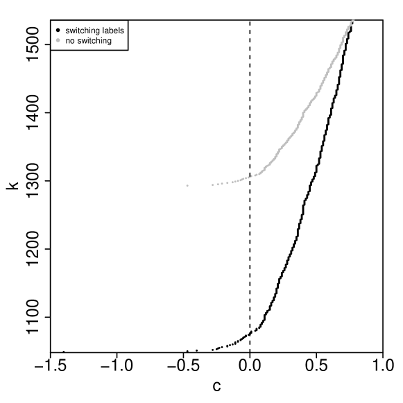
(a) Randomization inference

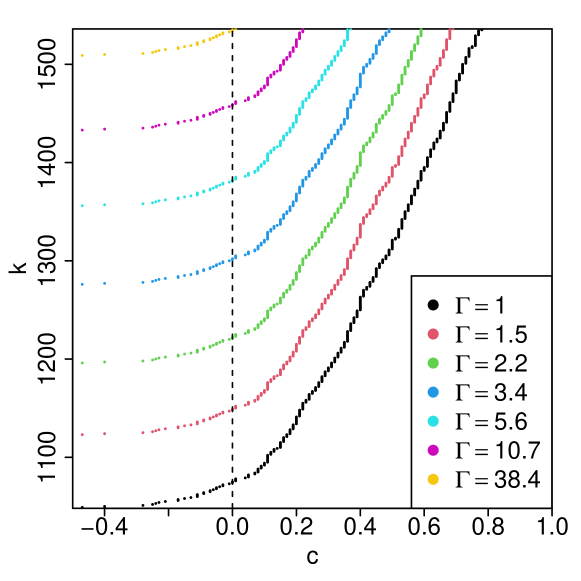
(b) Sensitivity analysis

Figure 1: $90\%$ lower confidence limits for quantiles of individual effects The left figure shows the lower confidence limits for quantiles of effects assuming there is no hidden confounding, i.e., the study reduces a SCRE, using either the original matched data or the one with switched treatment labels and changed outcome signs. The right figure shows the lower confidence limits for quantiles of individual effects under various sensitivity models indexed by different $\Gamma$’s using the data with switched treatment labels and changed outcome signs.

We first assume that matching has taken into account all confounding, under which the units within each matched set have the same probability to smoke. In this case, the matched observational study essentially reduces to a SCRE, for which we apply the randomization inference in §3–4 with the stratified Wilcoxon rank sum statistic. Figure 1(a) shows the $90\%$ lower confidence limits for all quantiles of individual effects, using both the original dataset and the one with switched treatment labels and changed outcome signs. Specifically, for each point in 1(a), its $x$-axis value denotes the lower confidence limit for the individual effect at rank its $y$-axis value. We omit those noninformative minus infinite lower confidence limits for $\tau_{(k)}$’s with small $k$. From Figure 1(a), it is obvious that treatment label switching helps provide more informative confidence intervals for quantiles of individual effects. Moreover, these intervals are simultaneously valid, as implied by Remark 2. With label switching, the $90\%$ lower confidence limit for the individual effect at rank $1076$ is 0.01. This implies that, with $90\%$ confidence level, at least $30\%$ of the units have positive effects, or equivalently smoking would cause higher blood cadmium level for at least $30\%$ of the units in the study.

We then consider sensitivity analysis, since the previous randomization inference pretending the study is a SCRE may be invalid due to the existence of unmeasured confounding. We apply the sensitivity analysis for quantiles of individual effects in §5 to the observed data with switched treatment labels and changed outcome signs. Figure 1(b) shows the $90\%$ lower confidence limits for all quantiles of individual effects under various sensitivity models with biases ranging from $1.0$ to $38.4$. These values of $\Gamma$, $1.0$, $1.5$, $2.2$, $3.4$, $5.6$, $10.7$ and $38.4$, are actually the largest values of $\Gamma$ such that the resulting confidence intervals for the $70\%$, $75\%$, $80\%$, $85\%$, $90\%$, $95\%$ and $100\%$ quantiles of individual effects do not cover zero. For example, when the bias in the treatment assignment is at most 2.2, the individual effect at rank 1229, i.e., $80\%$ quantile, is positive at significance level $0.1$, which implies that smoking would cause higher blood cadmium level for at least $20\%$ of the units in the study. Equivalently, we say the $80\%$ quantile of individual effect is significant for biases up to 2.2. From Rosenbaum (2017, Chapter 9), intuitively, a bias of magnitude 2 or 5 corresponds to an unobserved covariate that could produce a 3-fold or 9 fold increase in the odds of smoking, and 5-fold or 11-fold increase in the odds of a positive pair difference in cadmium levels. Since such a strong confounding is unlikely to exist, especially after taking into account those observed covariates in matching, we believe that smoking causes higher blood cadmium level for a non-negligible proportion of units, and the causal conclusion is robust to unmeasured confounding.

Conclusion

We studied nonparametric randomization-based inference and sensitivity analysis for quantiles of individual effects. We focused on alternative hypotheses that favor larger treatment effects. We can straightforwardly extend it to deal with alternative hypotheses that favor smaller treatment effects, by switching treatment labels or changing outcome signs. We can also conduct two-sided testing by combining the two one-sided testings using Bonferroni’s method (Cox 1977).

Our inference utilizes rank-based test statistics, and is applicable to both stratified randomized experiments and matched observational studies. Our inference is actually a costless addition to the conventional randomization inference and sensitivity analysis assuming constant treatment effects, and thus should always be encouraged in practice. The inference results can be conveniently visualized and interpreted, and a publicly available R package has also been developed.

It will be interesting to further incorporate pretreatment covariates to either improve the inference efficiency (Rosenbaum 2002c; Lin 2013) or consider conditional quantiles of individual treatment effects (Fan and Park 2010). We leave them for future research.

Supplementary material

Supplementary material available at Biometrika online includes simulation studies, proofs of all theorems and additional technical details. An R package implementing the proposed methods is available at https://github.com/Yongchang-Su/QIoT/.

Supplementary Material to “Treatment Effect Quantiles in Stratified Randomized Experiments and Matched Observational Studies”

§A1 conducts finite-sample sensitivity analysis, which is exact for matched pair studies but generally conservative. §A2 gives the details for the algorithms used to calculate valid $p$-values. §A3 conducts simulation studies, comparing various optimization algorithms and illustrating the power gain from Stephenson rank statistics and treatment label switching. §A4 gives the proofs of all propositions and theorems, as well as some technical remarks. §A5 gives additional technical details for optimizations.

Finite-sample sensitive analysis

Here we consider performing finite-sample valid sensitivity analysis. We first construct a finite-sample upper bound of $G_{\Gamma}(\cdot)$ that has a simple analytical expression and is easy to approximate by Monte Carlo. For each set $s$, let $\xi_{s1}<\ldots<\xi_{sm_{s}}$ be the unique values of the transformed ranks $\{\phi_{s}(1),\ldots,\phi_{s}(n_{s})\}$, and $g_{si}=\sum_{j=1}^{n_{s}}\mathbbm{1}\{\phi_{s}(j)\geq\xi_{si}\}$. For $\xi_{s,i-1}<c\leq\xi_{si}$ and any constant ${y}_{s}\in\mathbb{R}^{n_{s}}$, we can verify that, under the sensitivity model with bias at most $\Gamma$, $t_{s}({Z}_{s},{y}_{s})$ has at most probability $g_{si}\Gamma/\{(n_{s}-g_{si})+g_{si}\Gamma\}$ to be no less than $c$. This motivates us to define mutually independent random variables $(\overline{T}_{1},\ldots,\overline{T}_{S})$ with probability mass functions:

$$\text{Pr}\left(\overline{T}_{s}=\xi_{si}\right) =\frac{g_{si}\Gamma}{(n_{s}-g_{si})+g_{si}\Gamma}-\frac{g_{s,i+1}\Gamma}{(n_{s}-g_{s,i+1})+g_{s,i+1}\Gamma},\quad(i=1,2,\ldots,m_{s}),$$ (A1)

where $g_{s,m_{s}+1}$ is defined to be zero. By the mutual independence of treatment assignments across matched sets, the stratified rank score statistic $t({Z},{y})$ must be stochastically smaller than or equal to $\sum_{s=1}^{S}\overline{T}_{s}$. Therefore, the tail probability of $\sum_{s=1}^{S}\overline{T}_{s}$, denoted by $\overline{G}_{\Gamma}(\cdot)$, must be an upper bound of $G_{\Gamma}(\cdot)$ in (19). This further helps us construct finite-sample valid $p$-values for testing null hypotheses on quantiles of individual treatment effects under sensitivity models.

Theorem A1.

Under the sensitivity model with bias at most $\Gamma$ as in Definition 3, the following two $p$-values

$$\overline{p}_{k,c,\Gamma}\equiv\overline{G}_{\Gamma}(t_{k,c})\ \leq\ \overline{p}_{k,c,\Gamma}^{\prime}\equiv\overline{G}_{\Gamma}(t^{\prime}_{k,c})$$ (A2)

are both valid for testing the null hypothesis $H_{k,c}$ in (6), where $\overline{G}_{\Gamma}(\cdot)$ is the tail probability of $\sum_{s=1}^{S}\overline{T}_{s}$ with mutually independent $\overline{T}_{s}$’s defined in (A1). That is, if the null hypothesis $H_{k,c}$ holds and the bias in the treatment assignment is bounded by $\Gamma$, then, for any $\alpha\in(0,1)$,

$$\text{Pr}(\overline{p}_{k,c,\Gamma}^{\prime}\leq\alpha)\leq\text{Pr}(\overline{p}_{k,c,\Gamma}\leq\alpha)\leq\alpha.$$

As commented in §A4.11, in a matched pair study with $n_{1}=\ldots=n_{S}=2$, $\overline{G}_{\Gamma}(\cdot)$ becomes the same as $G_{\Gamma}(\cdot)$, i.e., the optimization in (19) has a closed-form analytical solution. However, for general matched studies with $n_{s}\geq 2$, $\overline{G}_{\Gamma}(\cdot)$ is generally different from $G_{\Gamma}(\cdot)$ and may be too conservative. In §5.3, we construct an asymptotic approximation for $G_{\Gamma}(\cdot)$ that is sharper than $\overline{G}_{\Gamma}(\cdot)$ and can thus lead to more powerful sensitivity analysis in large samples.

Analogous to Theorems 3 and 6, we can then invert the tests to construct simultaneously valid confidence sets for the quantiles of individual effects $\tau_{(k)}$’s and numbers of units with effects greater than any threshold $n(c)$’s. We summarize the results in the following theorem.

Theorem A2.

Under the sensitivity model with bias at most $\Gamma$, the $p$-value $\overline{p}_{k,c,\Gamma}$ is increasing in $c$ and decreasing in $k$. Moreover, for any $\alpha\in(0,1)$,

1. $\overline{\mathcal{I}}_{\alpha}(k)\equiv\{c:\overline{p}_{k,c,\Gamma}>\alpha,c\in\mathbb{R}\}$ is a $1-\alpha$ confidence set for $\tau_{(k)}$, and it must be an interval of the form $(\underline{c},\infty)$ or $[\underline{c},\infty)$, with $\underline{c}=\inf\{c:\overline{p}_{k,c,\Gamma}>\alpha\}$;

2. $\overline{\mathcal{S}}_{\alpha}(c)\equiv\{N-k:\overline{p}_{k,c,\Gamma}>\alpha,0\leq k\leq N\}$ is a $1-\alpha$ confidence set for $n(c)$, and it must have the form of $\{j:N-\overline{k}\leq j\leq N\}$, with $\overline{k}=\sup\{k:\overline{p}_{k,c,\Gamma}>\alpha\}$;

3. the intersection of all $1-\alpha$ confidence sets for $\tau_{(k)}$’s, viewed as a confidence set for ${\tau}$, is the same as that for $n(c)$’s, and they have the following equivalent forms:

   $$\big{\{}{\delta}:\delta_{(k)}\in\overline{\mathcal{I}}_{\alpha}(k),1\leq k\leq N\big{\}} =\Big{\{}{\delta}:\sum_{i=1}^{N}\mathbbm{1}(\delta_{i}>c)\in\overline{\mathcal{S}}_{\alpha}(c),c\in\mathbb{R}\Big{\}}=\bigcap_{k,c:\overline{p}_{k,c,\Gamma}\leq\alpha}\mathcal{H}_{k,c}^{\complement}.$$

   Moreover, the resulting confidence set covers the true individual treatment effect vector ${\tau}$ with probability at least $1-\alpha$, i.e., $\text{Pr}({\tau}\in\bigcap_{k,c:\overline{p}_{k,c,\Gamma}\leq\alpha}\mathcal{H}_{k,c}^{\complement})\geq 1-\alpha.$

Remark A1.

Theorem A2 also holds for the easier-to-calculate $p$-value $\overline{p}_{k,c,\Gamma}^{\prime}$.

Details for Algorithms Used to Calculate Valid $p$-values

In this section we introduce the details for the algorithms used to solve the integer programming in (13) and the relaxed linear programming in (14), which can then provide valid $p$-values for testing null hypotheses on quantiles of individual treatment effects. We first introduce the piecewise-linear optimization for the integer programming in (13), which can be solved by the Gurobi optimizer. We then introduce two algorithms adopted from the literature on the multiple-choice knapsack problem. The first is a greedy algorithm that can efficiently solve the relaxed linear programming in (14) in linear time, and the second is the dynamic programming algorithm that can solve the integer programming in (13) in polynomial time.

A2.1 Piecewise-linear optimization

The integer programming problem in (13) can be equivalently formulated as a piecewise-linear optimization problem. Specifically, for each $1\leq s\leq S$ and $0\leq x\leq n_{s}$, define

$$f_{s,c}(x)=\mathbbm{1}(x=0)t_{s,c}(0)+\sum_{j=0}^{n_{s}-1}\mathbbm{1}(j<x\leq j+1)[t_{s,c}(j)+\{t_{s,c}(j+1)-t_{s,c}(j)\}(x-j)].$$

The minimum objective value from (13) is then equivalently

$$\min_{l\in\mathcal{K}_{{n}}(N-k)}\sum_{s=1}^{S}f_{s,c}(l_{s})=\min_{l\in\mathcal{R}_{{n}}(N-k)}\sum_{s=1}^{S}f_{s,c}(l_{s}),$$ (A3)

where $\mathcal{K}_{{n}}(N-k)$ is defined as in (10), and $\mathcal{R}_{{n}}(N-k)$ is defined the same as $\mathcal{K}_{{n}}(N-k)$ but without the integer constraints. Besides, the objective function in (A3) can be non-convex. In §A5.2, we prove the equality in (A3) and give a numerical example showing the non-convexity of the objective function. We also investigate the performance of Gurobi optimizer for this piecewise-linear optimization in §A3.1.

A2.2 Greedy Algorithm for solving the relaxed linear programming problem

We first introduce some notation to give an equivalent form for the optimization in (12). By definition, we can verify that, for each $s$, $t_{s,c}(0)\geq t_{s,c}(1)\geq\ldots\geq t_{s,c}(n_{s})$. Define $\Delta_{s,c}(j)\equiv t_{s,c}(j-1)-t_{s,c}(j)\geq 0$ for all $s,j$. Then the optimization in (12) reduces to

$$\inf_{{\delta}\in\mathcal{H}_{k,c}}t({Z},{Y}-{Z}\circ{\delta}) =\sum_{s=1}^{S}t_{s,c}(0)-\max_{(l_{1},\ldots,l_{S})\in\mathcal{K}_{{n}}(N-k)}\sum_{s=1}^{S}\sum_{j=1}^{l_{s}}\Delta_{s,c}(j).$$ (A4)

Consequently, to get the valid $p$-value $p_{k,c}$, it suffices to maximize $\sum_{s=1}^{S}\sum_{j=1}^{l_{s}}\Delta_{s,c}(j)$ over $(l_{1},\ldots,l_{S})\in\mathcal{K}_{{n}}(N-k)$. The naive greedy algorithm solves this maximization by making locally optimal choice at each stage when $N-k$ increases from $0$ to $N$. However, this may lead to sub-optimal solutions; see §A5.1 for a numerical example. More importantly, it may invalidate the resulting $p$-value.

The naive greedy algorithm fails mainly because $\Delta_{s,c}(j)$ can increase as $j$ increases, and thus searching only the local optimum will miss the correct solution. To overcome this drawback, we propose to transform the sequence of $\Delta_{s,c}(j)$’s for each $s$ such that the resulting sequence is monotone decreasing and its cumulative sums dominate that of the original sequence. We formally define such a transformation below.

Definition 4.

A function $\Psi(\cdot)$ that maps a vector to a vector of the same length is called a monotone dominating transformation, if for any $m\geq 1$ and any vector ${a}=(a_{1},\ldots,a_{m})^{\top}\in\mathbb{R}^{m}$, the transformation $\Psi({a})=(\Psi_{1}({a}),\ldots,\Psi_{m}({a}))^{\top}\in\mathbb{R}^{m}$ satisfies that (i) $\Psi_{1}({a})\geq\Psi_{2}({a})\geq\ldots\geq\Psi_{m}({a})$ and (ii) $\sum_{i=1}^{j}\Psi_{i}({a})\geq\sum_{i=1}^{j}a_{i}$ for $1\leq j\leq m$.

Let ${\Delta}_{s,c}(\overline{j})=(\Delta_{s,c}(1),\ldots,\Delta_{s,c}(j))$ for $1\leq s\leq S$, $1\leq j\leq n_{s}$ and $c\in\mathbb{R}$. From the two properties in Definition 4, for any monotone dominating transformation $\Psi(\cdot)$,

$$\Psi_{1}\left({\Delta}_{s,c}\left(\overline{n_{sk}}\right)\right)\geq\Psi_{2}\left({\Delta}_{s,c}\left(\overline{n_{sk}}\right)\right)\geq\ldots\geq\Psi_{n_{sk}}\left({\Delta}_{s,c}\left(\overline{n_{sk}}\right)\right),\quad(1\leq s\leq S)$$ (A5)

and for any $(l_{1},\ldots,l_{S})\in\mathcal{K}_{{n}}(N-k)$,

$$\sum_{s=1}^{S}\sum_{j=1}^{l_{s}}\Delta_{s,c}(\overline{j})\leq\sum_{s=1}^{S}\sum_{j=1}^{l_{s}}\Psi_{j}\left({\Delta}_{s,c}\left(\overline{n_{sk}}\right)\right).$$ (A6)

Importantly, with the transformed $\Delta_{s,c}(j)$’s, (A5) guarantees that the naive greedy algorithm can achieve the global maximum of the objective function on the right hand side of (A6) over $l\in\mathcal{K}_{{n}}(N-k)$, and (A6) guarantees that the achieved global maximum must be no less than the target maximum of the objective function on the left hand side of (A6). This further helps provide conservative but still valid $p$-value for testing $H_{k,c}$.

The remaining question is how to optimally construct a monotone dominating transformation. It turns out the optimal transformation has a simple form and is easy to compute. Define $\tilde{\Psi}:{a}=(a_{1},\ldots,a_{m})^{\top}\rightarrow\tilde{\Psi}({a})=(\tilde{\Psi}_{1}({a}),\ldots,\tilde{\Psi}_{m}({a}))$ recursively as:

$$\tilde{\Psi}_{i}({a}) =\begin{cases}\max_{1\leq j\leq m}j^{-1}\sum_{t=1}^{j}a_{t},&\text{for }i=1,\\ \max_{i\leq j\leq m}(j-i+1)^{-1}{\color[rgb]{0,0,0}\left\{\sum_{t=1}^{j}a_{t}-\sum_{t=1}^{i-1}\tilde{\Psi}_{t}({a})\right\}},&\text{for }i=2,\ldots,m.\end{cases}$$ (A7)

The following proposition establishes the optimality of $\tilde{\Psi}(\cdot)$.

Proposition A1.

The mapping $\tilde{\Psi}(\cdot)$ defined in (A7) is a monotone dominating transformation as in Definition 4. Moreover, for any $m\geq 1$, ${a}\in\mathbb{R}^{m}$ and any monotone dominating transformation $\Psi(\cdot)$, $\sum_{i=1}^{j}\tilde{\Psi}_{i}({a})\leq\sum_{i=1}^{j}\Psi_{i}({a})$ for all $1\leq j\leq m$.

We are now ready to describe the greedy algorithm with the optimal monotone dominating transformation $\tilde{\Psi}(\cdot)$ in (A7). Surprisingly at the first glance and as discussed in detail later, the greedy algorithm actually solves the linear programming problem in (14). We summarize the algorithm below.

Algorithm 1.

Greedy algorithm for the linear programming problem in (14).

Input: observed data $(Y_{s},Z_{s})$ for all $s$, the null hypothesis of interest $H_{k,c}$, and values of $t_{s,c}(j)$

and $\Delta_{s,c}(j)$ for stratum $1\leq s\leq S$ and $1\leq j\leq n_{sk}$;

For each stratum $s$, perform the transformation $\tilde{\Delta}_{sk,c}(\overline{n_{sk}})\equiv\tilde{\Psi}(\Delta_{s,c}(\overline{n_{sk}}))$;

Pool all the transformed elements into $\mathcal{T}_{k,c}\equiv\{\tilde{\Delta}_{sk,c}(j):1\leq j\leq n_{sk},1\leq s\leq S\}$;

Output: $t_{k,c}^{\prime}=\sum_{s=1}^{S}t_{s,c}(0)-\text{sum of the largest $N-k$ elements of }\mathcal{T}_{k,c}.$

Below we give several remarks regarding Algorithm 1. First, the final solution has a simple form, involving only sorting and summing elements of $\mathcal{T}_{k,c}$. This is due to the property (i) in Definition 4 for the monotone dominating transformation. As commented in §A5.4, the computational complexity of the greedy algorithm is $O(N\log N+N\max_{s}n_{s})$, while that for solving a general linear programming problem involving $N$ variables is at least $O(N^{2+\epsilon})$ with the latest improvement of $\epsilon=1/18$ [Jiang et al., 2020].

Second, the greedy algorithm here actually solves the linear programming problem in (14); we give a proof in §A5.3. As demonstrated in §A5.3, for each stratum $s$, $\{(j,\sum_{i=1}^{j}\tilde{\Delta}_{sk,c}(i)):0\leq j\leq n_{sk}\}$ from the optimal transformation in (A7) actually forms the upper convex hull of $\{(j,\sum_{i=1}^{j}\Delta_{s,c}(i)):0\leq j\leq n_{sk}\}$. Consequently, the greedy algorithm we introduce here is essentially equivalent to the greedy algorithm for the linear programming relaxation of multiple-choice knapsack problems [Kellerer et al., 2004, Page 320]. Moreover, the computational complexity of the greedy algorithm can be further reduced to $O(N)$ by employing algorithms in Dyer [1984] and Zemel [1984]. Our R package implements the $O(N)$ algorithm.

Third, when the rank transformations $\phi_{s}(\cdot)$’s in (4) is a concave function, the sequence $\{\Delta_{s,c}(j)\}$ will itself be decreasing in $j$, and it will be invariant under the optimal transformation $\tilde{\Psi}(\cdot)$. Thus, for stratified rank score statistics with concave transformations, which include the stratified Wilcoxon rank sum statistic as a special case, the greedy algorithm solves exactly the integer linear programming in (13). However, the rank transformations in stratified Stephenson rank sum statistics are generally not concave. Instead, they are always convex, under which the monotone dominating transformation is necessary to ensure the validity of the resulting $p$-values. We relegate the technical details to §A5.5.

A2.3 Dynamic programming for solving the integer linear programming problem

Here we adopt the dynamic programming algorithm that can solve the multiple-choice knapsack problem in pseudopolynomial time as shown by Dudziński and Walukiewicz [1987]; see also Kellerer et al. [2004, Page 329–331]. Similar to §A2.2, we consider the equivalent form in (A4) and aim to maximize $\sum_{s=1}^{S}\sum_{j=1}^{l_{s}}\Delta_{s,c}(j)$ over $(l_{1},\ldots,l_{S})\in\mathcal{K}_{{n}}(N-k)$. For $1\leq b\leq S$ and nonnegative integer $d$, define $m_{b}(d)$ as the maximum value of the objective function but restricted to the first $b$ strata and with the constraint that the sum of $l_{s}$’s is bounded by $d$, i.e.,

$$m_{b}(d)=\max\Big{\{}\sum_{s=1}^{b}\sum_{j=1}^{l_{s}}\Delta_{s,c}(j):(l_{1},\ldots,l_{b})\in\mathbb{Z}^{b},0\leq l_{s}\leq n_{s}\text{ for all }s,\sum_{s=1}^{b}l_{s}\leq d\Big{\}}.$$ (A8)

Equivalently, $\sum_{s=1}^{b}t_{s,c}(0)-m_{b}(d)$ is the minimum value of the rank sum test statistic for the first $b$ strata under the constraint that there are at most $d$ units with individual effects greater than $c$. We further define $m_{0}(d)=0$ for all nonnegative integer $d$. We can verify that $m_{b}(d)$’s satisfy the following recursive formula: for $1\leq b\leq S$ and nonnegative integer $d$,

$$m_{b}(d)=\max\big{\{}m_{b-1}(d-i)+\sum_{j=1}^{i}\Delta_{b,c}(j):i=0,1,\ldots,\min\{n_{b},d\}\big{\}}.$$ (A9)

Importantly, $m_{S}(N-k)$ gives the maximum value of the objective function on the right hand side of (A4), which equivalently provides the optimal objective value $t_{k,c}$ for the integer linear programming in (13). We summarize the algorithm below.

Algorithm 2.

Dynamic programming for the integer linear programming problem in (13).

Input: observed data $(Y_{s},Z_{s})$ for all $s$, the null hypothesis of interest $H_{k,c}$, and values of $t_{s,c}(j)$

and $\Delta_{s,c}(j)$ for stratum $1\leq s\leq S$ and $1\leq j\leq n_{sk}$;

Initialize $m_{0}(0)=m_{0}(1)=\ldots=m_{0}(N-k)=0$;

For $s=1$ to $s=S$

Calculate $m_{s}(0),m_{s}(1),\ldots,m_{s}(N-k)$ using the recursive formula in (A9);

Output: $t_{k,c}=\sum_{s=1}^{S}t_{s,c}(0)-m_{S}(N-k).$

In Algorithm 2, at each iteration and for calculating each $m_{s}(d)$, we calculate at most $n_{s}+1$ cumulative sums of $\Delta_{s,c}(j)$ and perform at most $n_{s}+1$ summations to complete the recursion in (A9). Therefore, the computational complexity of the dynamic programming is at most of order $(N-k)\sum_{s=1}^{S}(n_{s}+1)\leq 2(N-k)N\leq 2N^{2}$. This indicates that we can solve exactly the integer programming in (13) in polynomial time, with exponent of the sample size being at most $2$. Note that a general multiple-choice knapsack problem is NP-hard. Here we have a polynomial-time algorithm because the total cost in our problem in (13) is always bounded by $N$.

It is also worth noting that the dynamic programming with $k=0$ calculates simultaneously $t_{j,c}$ for all $0\leq j\leq N$, which then leads to $p$-values $p_{j,c}$ for all $0\leq j\leq N$. As discussed in Theorem 3(ii), these $p$-values immediately provide confidence sets for $n(c)$, i.e., the number of units with treatment effects greater than $c$.

Simulation studies

A3.1 Computation cost for getting the valid $p$-values

We consider a SCRE with $S$ ($=100,500,1000,2000,3000$) strata of equal size $n$ ($=50,100,200$), where each stratum has half of its units assigned to treatment. We use the stratified Stephenson rank sum statistic with $h_{s}=6$ for all $s$. We simulate the potential outcomes $Y_{si}(1)=Y_{si}(0)$ for all $s$ and $i$ as i.i.d. samples from the standard Gaussian distribution. We consider testing the null hypothesis on the $90\%$ quantile of individual treatment effects, or more precisely, $H_{k,0}:\tau_{(k)}\leq 0$ with $N=nS$ and $k=0.9N$. We consider the following algorithms for achieving the minimum test statistic value $t_{k,0}$ or $t_{k,0}^{\prime}$ from the integer linear programming (ILP) in (13) or the linear programming (LP) in (14):

1. the greedy algorithm for the LP in (14) (denoted by LP-GT) as described in §A2.2,

2. the dynamic programming for the ILP in (13) (denoted by ILP-DP) as described in §A2.3,

3. Gurobi optimizer for the LP in (14) (denoted by LP-Gurobi),

4. Gurobi optimizer for the ILP in (13) (denoted by ILP-Gurobi),

5. Gurobi optimizer for the piecewise linear optimization with integer constraints (denoted by IPWL-Gurobi) as described in §A2.1,

6. Gurobi optimizer for the piecewise linear optimization without the integer constraints (denoted by PWL-Gurobi) as described in §A2.1.

For the integer programming, our Gurobi programming involves $N+S$ binary integer variables and $S+1$ additional linear constraints. For the piecewise linear optimization without the integer constraints, our Gurobi programming involves $S$ variables with given lower and upper bounds, $1$ additional linear constraint, and $S$ piecewise linear constraints.

Table A1 shows the run time of the six algorithms under different choices of $(n,S)$, taking median over 100 simulated datasets, where we exclude the time for getting $t_{s,0}(l)$’s for all $s$ and $l$. It should be noted that the Gurobi optimizer incorporates an error tolerance mechanism, which implies that the solutions provided by Gurobi are accurate within certain predetermined numeric tolerance. In contrast, both the greedy algorithm and dynamic programming solve the corresponding linear and integer programming problems exactly, subject to the level of numerical precision. From our simulation, the average absolute values of the relative differences of LP-GT, LP-Gurobi, ILP-Gurobi, IPWL-Gurobi and PWL-Gurobi from ILP-DP, scaled by $10^{4}$, are, respectively, $3.94$, $3.94$, $3.28$, $3.50$ and $3.32$. These show that the solutions from the relaxed linear programming are comparable to that from Gurobi optimizations for the integer programming.

Table A1 shows the run time of the previously listed six algorithms. First, LP-GT is much faster than the other five algorithms. Second, LP-Gurobi and ILP-Gurobi take about the same time, and both of them are much faster than IPWL-Gurobi and PWL-Gurobi. Third, the dynamic programming performs well with moderate sample sizes, but its computation time increases significantly as the sample size grows. However, it is worth mentioning that a single run of the dynamic programming can efficiently calculate the $p$-values $p_{0,c},p_{1,c},\ldots,$ and $p_{N,c}$ at the same time, which will then provide confidence sets for $n(c)$. Therefore, it can be preferred when we are particularly interested in the number, or equivalently the proportion, of units with effects greater than a given threshold; see also the discussion at the end of §A2.3.

Table A1: Run time in seconds of the six algorithms, linear programming (LP) solved by greedy algorithm with the optimal transformation (GT) and Gurobi, integer linear programming (ILP) solved by dynamic programming (DP) and Gurobi, and piecewise-linear (PWL) optimization with and without integer constraints solved by Gurobi, for testing null hypothesis on the $90\%$ quantile of individual effects under various values of $(n,S)$, taking median over 100 simulated datasets. The simulation is conducted using AMD Ryzen 5 5600X 3.70 GHz processor.

Stratum size	Strata number	LP-GT	LP-Gurobi	ILP-DP	ILP-Gurobi	IPWL-Gurobi	PWL-Gurobi
	$S=100$	0.00	0.01	0.01	0.03	0.25	0.24
	$S=500$	0.00	0.06	0.28	0.11	0.73	0.58
$n=50$	$S=1000$	0.01	0.17	1.14	0.22	1.78	1.23
	$S=2000$	0.02	0.44	4.70	0.51	5.85	3.00
	$S=3000$	0.03	0.88	10.58	0.96	11.49	5.66
	$S=100$	0.00	0.02	0.03	0.04	0.25	0.24
	$S=500$	0.01	0.12	0.72	0.20	1.66	1.44
$n=100$	$S=1000$	0.02	0.31	3.00	0.41	3.03	2.68
	$S=2000$	0.05	1.01	12.23	1.05	8.69	6.75
	$S=3000$	0.08	2.08	27.60	2.02	39.18	47.03
	$S=100$	0.01	0.03	0.08	0.08	0.73	0.68
	$S=500$	0.03	0.22	2.21	0.37	3.88	5.58
$n=200$	$S=1000$	0.07	0.61	9.06	0.93	11.38	7.88
	$S=2000$	0.14	1.93	36.59	2.30	43.44	50.54
	$S=3000$	0.22	3.84	82.78	4.39	41.93	43.13

We further consider a large dataset from Lalive et al. [2006] on studying the change in unemployment benefits in Austria. Similar to Yu and Rosenbaum [2022], we focus on men who were not temporarily laid off, pooling the three groups with increased benefits. We consider the duration of unemployment as the outcome of interest, and conduct $1:6$ matching [Ho et al., 2011] based on the following covariates: age, wage in prior job, an indicator of at least 3 years of work in the past 5 years, whether the job was an apprenticeship, married or not, divorced or not, education in three levels, whether or not the previous job was a blue collar job, a seasonal job, a manufacturing job. We allow control units to be matched with multiple treated units. The in total 55619 units are then divided into 22111 matched sets, each of which contains 1 treated unit and 6 control units. We then construct $80\%$ confidence intervals for the $95\%$, $90\%$, $85\%$, $80\%$ quantiles of individual treatment effects using our approach in §4 with the Stephenson rank sum statistic and $h_{s}=5$ for all matched sets, pretending that the matched observational study is a SCRE; we can also conduct sensitivity analysis as in §5. We compare all the algorithms in Table A1. Table A2 shows the computation time of the algorithms for each of these quantiles, excluding the time for approximating the null distribution of the rank statistic, which needs to be done only once and can be shared for all quantiles, takes $14.19$ minutes here using $10^{5}$ Monte Carlo draws, and can also be approximated using a normal approximation as in §5.3. From Table A2, first, the greedy algorithm takes the shortest run time, while IPWL-Gurobi takes the longest run time. In particular, the IPWL-Gurobi takes about 1 hour to get the confidence interval for the $80\%$ quantile of individual effects, while the greedy algorithm takes about $1$ minute. Second, ILP-DP, PWL-Gurobi and IPWL-Gurobi tend to take longer run time when we consider smaller quantiles of individual effects, while the run time of the other three algorithms is quite stable across all quantiles.

From the above, the greedy algorithm can be preferable when analyzing large datasets or using statistics with concave rank transformation for which the greedy algorithm is also exact for the integer programming. When we are particularly interested in the number of units with effects passing a given threshold, the dynamic programming algorithm can be preferred. In other general cases, we will suggest the Gurobi optimization for the integer programming.

Table A2: Run time in minutes of six algorithms in Table A1 for obtaining $80\%$ confidence intervals of the $95\%$, $90\%$, $85\%$, $80\%$ quantiles of individual treatment effects.

Quantile	$95\%$	$90\%$	$85\%$	$80\%$
LP-GT	1.13	1.07	1.08	1.07
LP-Gurobi	2.53	2.41	2.43	2.46
ILP-DP	4.54	8.04	11.49	15.40
ILP-Gurobi	2.76	2.61	2.60	2.58
PWL-Gurobi	7.18	5.68	26.76	27.42
IPWL-Gurobi	23.98	24.94	83.09	64.01

A3.2 Choice of test statistics

We consider a SCRE with $S=200$ strata of equal size $n$ ($=10,20,50$), and randomly assign half of the units within each stratum to treatment. We simulate the potential outcomes as i.i.d. samples from the following model:

$$Y_{si}(0)\sim\mathcal{N}(0,1),\quad Y_{si}(1)=\tau+Y_{si}(0)+\sigma\epsilon_{si},\quad\epsilon_{si}\sim\mathcal{N}(0,1),\quad\epsilon_{si}\perp\!\!\!\perp Y_{si}(0),$$ (A10)

where we choose $\tau$ to be $0$ or $1$. Note that all strata have equal sizes. We consider stratified Stephenson rank sum statistics with $h_{1}=\ldots=h_{S}=h$ for some $h\geq 2$. To compare the power under various choice of $h$, we focus on inferring the number of units with positive effects $n(0)$, and use the greedy algorithm to calculate the valid $p$-values.

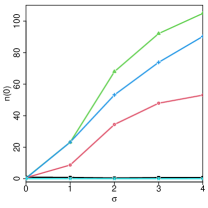
(a)

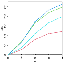
(b)

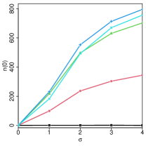
(c)

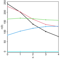
(d)

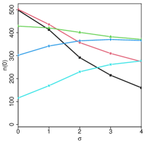
(e)

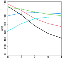
(f)

Figure A1: $90\%$ lower confidence limits for $n(0)$ under various Stephenson rank statistics and strata sizes, averaging over 100 simulations. The top and bottom rows are for $\tau=0$ and 1, respectively.

Figure A1 shows the $90\%$ lower confidence limits of $n(0)$ using various stratified Stephenson rank sum statistics under different strata sizes, averaging over 100 simulated datasets, when the expected average effect $\tau$ equals 0 and 1. Note that when $h>n$, the Stephenson ranks will become constant zero and the resulting test will lose power. We consider only the choice of $h$ such that $h<n$. From Figure A1, moderately large $h$ compared to $n$ can help improve the power for inferring $n(0)$. For example, when $n=50$, using the Stephenson rank with $h=6$ can provide more informative lower confidence limit for $n(0)$ on average than using the Stephenson rank with $h=2$, which reduces to the Wilcoxon rank. However, when $h$ is overly large compared to $n$, it can deteriorate the power of our inference. In practice, we suggest to use the Stephenson rank with moderate parameter compared to the stratum size. We leave a more detailed theoretical investigation for future study.

A3.3 Treatment label switching for matched observational study

We consider a matched observational study with $S=200$ matched sets, each of which contains 1 treated unit and 9 control units. We generate the potential outcomes as i.i.d. samples from model (A10) with $(\tau,\sigma)=(1,0)$, i.e., the treatment has a constant effect 1. Moreover, following Rosenbaum [2002a], we consider the favorable situation where there is no hidden confounding, i.e., the study is essentially a SCRE. In this favorable situation with nonzero treatment effects, we wish to detect significant treatment effects and hope the detected effects to be insensitive to hidden confounding.

To illustrate the power gain from treatment label switching, we consider testing the null hypothesis $H_{k,0}:\tau_{(k)}\leq 0$ with $N=2000$ and $k=0.95N$ under sensitivity models. In particular, we consider using either the original data or that with switched treatment labels and changed outcome signs. We use the greedy algorithm to calculate the valid $p$-values. Table A3 shows the empirical power of the test using the stratified Stephenson rank sum statistic with $h_{1}=\ldots=h_{S}=4$ under various sensitivity models, based on 100 simulated datasets.

Table A3: Empirical power of two tests regarding the $90\%$ quantile of individual effects under various sensitivity models, averaging over 100 simulated datasets. One test uses the original data, while the other uses the data with switched treatment labels and changed outcome signs.

$\Gamma$	1	1.1	1.2	1.3	1.4	1.5	1.6	1.7	1.8
Switching labels	0.97	0.91	0.7	0.44	0.20	0.10	0.04	0.02	0.01
No switching	0.00	0.00	0.00	0.00	0.00	0.00	0.00	0.00	0.00

From Table A3, switching labels can greatly increase the power of the test. When $\Gamma=1$, i.e., there is no hidden confounding and the study reduces to a SCRE, the power of the test after label switching is almost 1, while that using the original data is about 0. As $\Gamma$ increases, we allow more amount of biases in the treatment assignment, and thus the power of the test decreases. Importantly, label switching still provides significant gain in power when $\Gamma>1$, making the study more robust to unmeasured confounding. Thus, for general matched observational studies with one treated and multiple control units within each matched set, we suggest to perform label switching as discussed in Remarks 5 and 8, which can bring significant power gain as demonstrated by Table A3.

Proof of Propositions, Theorems and Remarks

A4.1 Proof of Proposition 1

Under the SERE, $Z_{1}$, $Z_{2}$, $\ldots$, $Z_{S}$ are mutually independent, so it suffices to prove that $t_{s}({Z}_{s},{y}_{s})$ is distribution free within each stratum $s$, for $1\leq s\leq S$. For any ${y}_{s},{y}_{s}^{\prime}\in\mathbb{R}^{n_{s}}$, let $r_{si}=\text{rank}_{i}({y_{s}})$ and $r_{si}^{\prime}=\text{rank}_{i}({y}_{s}^{\prime})$ for $1\leq i\leq n_{s}$. By the property of the stratified rank score statistic in Definition 2, both ${r}_{s}=(r_{s1},r_{s2},\ldots,r_{sn_{s}})$ and ${r}^{\prime}_{s}=(r^{\prime}_{s1},r^{\prime}_{s2},\ldots,r^{\prime}_{sn_{s}})$ are permutations of $\{1,2,\ldots,n_{s}\}$. Thus, there must exist two permutations $\pi(\cdot)$ and $\pi^{\prime}(\cdot)$ of $\{1,2,\ldots,n_{s}\}$ such that $r_{s\pi(i)}=r^{\prime}_{s\pi^{\prime}(i)}=i$ for $1\leq i\leq n_{s}$. Consequently, we have $t_{s}({Z}_{s},{y}_{s})=\sum_{i=1}^{n_{s}}Z_{si}\phi_{s}(r_{si})=\sum_{i=1}^{n_{s}}Z_{s\pi(i)}\phi_{s}(i)$, and by the same logic $t_{s}({Z}_{s},{y}_{s}^{\prime})=\sum_{i=1}^{n_{s}}Z_{s\pi^{\prime}(i)}\phi_{s}(i)$. By Definition 1 of the SERE, $(Z_{s\pi(1)},\ldots,Z_{s\pi(n_{s})})$ follows the same distribution as $(Z_{s\pi^{\prime}(1)},\ldots,Z_{s\pi^{\prime}(n_{s})})$. Thus, $t_{s}({Z}_{s},{y}_{s})\sim t_{s}({Z}_{s},{y}^{\prime}_{s})$. From the above, Proposition 1 holds.

A4.2 Proof of Theorem 1

From Casella and Berger [2002, Theorem 8.3.27], $p_{k,c}=\sup_{{\delta}\in\mathcal{H}_{k,c}}p_{{Z},{\delta}}$ is a valid $p$-value for testing $H_{k,c}$. Below we prove its equivalent forms in (9). It suffices to show that $t({Z},{Y}-{Z}\circ{\delta})$ can achieve its infimum over ${\delta}\in\mathcal{H}_{k,c}$. From the discussion in §3.2, the infimum of $t({Z},{Y}-{Z}\circ{\delta})$ over ${\delta}\in\mathcal{H}_{k,c}$ has an equivalent form shown in (12), which immediately implies that there exists $(\tilde{l}_{1},\tilde{l}_{2},\ldots,\tilde{l}_{S})\in\mathcal{K}_{{n}}(N-k)$ such that $\inf_{{\delta}\in\mathcal{H}_{k,c}}t({Z},{Y}-{Z}\circ{\delta})=\sum_{s=1}^{S}t_{s,c}(\tilde{l}_{s}).$ From Caughey et al. [2021, Theorem 3], there exists $\tilde{{\delta}}=(\tilde{{\delta}}_{1}^{\top},\ldots,\tilde{{\delta}}_{S}^{\top})^{\top}$ with $\tilde{{\delta}}_{s}\in\mathcal{H}^{s}_{n_{s},n_{s}-\tilde{l}_{s},c}$ for $1\leq s\leq S$ such that $t_{s,c}(\tilde{l}_{s})=t_{s}({Z}_{s},{Y}_{s}-{Z}_{s}\circ\tilde{{\delta}}_{s})$ for $1\leq s\leq S$. Therefore, we must have $\tilde{{\delta}}\in\mathcal{H}_{k,c}$ by definition, and

$$\inf_{{\delta}\in\mathcal{H}_{k,c}}t({Z},{Y}-{Z}\circ{\delta})=\sum_{s=1}^{S}t_{s,c}(\tilde{l}_{s})=\sum_{s=1}^{S}t_{s}({Z}_{s},{Y}_{s}-{Z}_{s}\circ\tilde{{\delta}}_{s})=t({Z},{Y}-{Z}\circ\tilde{{\delta}}).$$

From the above, Theorem 1 holds.

A4.3 Proof of Theorem 2 and Remark 1

To prove Theorem 2 and Remark 1, we introduce the following lemma.

Lemma A1.

Consider any given $n\geq 1$, any $z=(z_{1},\ldots,z_{n})\in\{0,1\}^{n}$ and any permutation $\pi$ of $\{1,2,\ldots,n\}$. We define the following three rank functions that rank units from $1$ to $n$ based on any given vector $y=(y_{1},\ldots,y_{n})\in\mathbb{R}^{n}$: for any $1\leq i\neq j\leq n$,

• $\text{rank}_{i}(y)<\text{rank}_{j}(y)$ if (i) $y_{i}<y_{j}$, or (ii) $y_{i}=y_{j}$ and $\pi_{i}<\pi_{j}$;

• $\overline{\text{rank}}_{i}(y)<\overline{\text{rank}}_{j}(y)$ if (i) $y_{i}<y_{j}$, (ii) $y_{i}=y_{j}$ and $z_{i}<z_{j}$, or (iii) $y_{i}=y_{j}$, $z_{i}=z_{j}$, and $\pi_{i}<\pi_{j}$;

• $\underline{\text{rank}}_{i}(y)<\underline{\text{rank}}_{j}(y)$ if (i) $y_{i}<y_{j}$, (ii) $y_{i}=y_{j}$ and $z_{i}>z_{j}$, or (iii) $y_{i}=y_{j}$, $z_{i}=z_{j}$, and $\pi_{i}<\pi_{j}$.

Let $\phi(\cdot)$ be any increasing function on $\{1,2,\ldots,n\}$, and define further $d(z,y)=\sum_{i=1}^{n}z_{i}\phi(\text{rank}_{i}(y))$, $\overline{d}(z,y)=\sum_{i=1}^{n}z_{i}\phi(\overline{\text{rank}}_{i}(y))$, and $\underline{d}(z,y)=\sum_{i=1}^{n}z_{i}\phi(\underline{\text{rank}}_{i}(y))$.

• For any $y=(y_{1},\ldots,y_{n})\in\mathbb{R}^{n}$, $\underline{d}(z,y)\leq d(z,y)\leq\overline{d}(z,y)$.

• For any finite positive real number $a$, $\overline{d}(z,y)\leq\underline{d}(z,y+az)$.

Note that the values of $\overline{d}(z,y)$ and $\underline{d}(z,y)$ do not depend on how we rank tied units with the same $z_{i}$’s; for simplicity, we use the same ranking as that in $\text{rank}_{i}(\cdot)$ for these units.

Proof of Lemma A1.

We first prove (1). For any $1\leq j\leq n$ with $z_{j}=1$, by definition,

$$\text{rank}_{j}(y) =\sum_{i=1}^{n}\mathbbm{1}(y_{i}<y_{j})+\sum_{i=1}^{n}\mathbbm{1}(y_{i}=y_{j})\mathbbm{1}(\pi_{i}\leq\pi_{j}),$$

$$\overline{\text{rank}}_{j}(y) =\sum_{i=1}^{n}\mathbbm{1}(y_{i}<y_{j})+\sum_{i=1}^{n}\mathbbm{1}(y_{i}=y_{j})\{(1-z_{i})+z_{i}\mathbbm{1}(\pi_{i}\leq\pi_{j})\},$$

$$\underline{\text{rank}}_{j}(y) =\sum_{i=1}^{n}\mathbbm{1}(y_{i}<y_{j})+\sum_{i=1}^{n}\mathbbm{1}(y_{i}=y_{j})z_{i}\mathbbm{1}(\pi_{i}\leq\pi_{j}).$$ (A11)

These immediately imply that, for any $j$ with $z_{j}=1$, $\underline{\text{rank}}_{j}(y)\leq\text{rank}_{j}(y)\leq\overline{\text{rank}}_{j}(y)$. Consequently, we must have $\underline{d}(z,y)\leq d(z,y)\leq\overline{d}(z,y)$.

We then prove (2). From (A4.3), for any $1\leq j\leq n$ with $z_{j}=1$,

$$\quad\ \underline{\text{rank}}_{j}(y+az)$$

$$=\sum_{i=1}^{n}\mathbbm{1}(y_{i}+az_{i}<y_{j}+a)+\sum_{i=1}^{n}\mathbbm{1}(y_{i}+az_{i}=y_{j}+a)z_{i}\mathbbm{1}(\pi_{i}\leq\pi_{j})$$

$$=\sum_{i=1}^{n}\{z_{i}+(1-z_{i})\}\mathbbm{1}(y_{i}+az_{i}<y_{j}+a)+\sum_{i=1}^{n}\mathbbm{1}(y_{i}=y_{j})z_{i}\mathbbm{1}(\pi_{i}\leq\pi_{j})$$

$$=\sum_{i=1}^{n}z_{i}\mathbbm{1}(y_{i}<y_{j})+\sum_{i=1}^{n}(1-z_{i})\mathbbm{1}(y_{i}<y_{j}+a)+\sum_{i=1}^{n}\mathbbm{1}(y_{i}=y_{j})z_{i}\mathbbm{1}(\pi_{i}\leq\pi_{j}).$$

From (A4.3), for any $1\leq j\leq n$ with $z_{j}=1$, we then have

$$\quad\ \underline{\text{rank}}_{j}(y+az)-\overline{\text{rank}}_{j}(y)$$

$$=\sum_{i=1}^{n}(1-z_{i})\mathbbm{1}(y_{i}<y_{j}+a)-\sum_{i=1}^{n}(1-z_{i})\mathbbm{1}(y_{i}<y_{j})-\sum_{i=1}^{n}(1-z_{i})\mathbbm{1}(y_{i}=y_{j}){\color[rgb]{0,0,0}\mathbbm{1}(\pi_{i}\leq\pi_{j})}$$

$${\color[rgb]{0,0,0}\geq}\sum_{i=1}^{n}(1-z_{i})\{\mathbbm{1}(y_{i}<y_{j}+a)-\mathbbm{1}(y_{i}\leq y_{j})\}\geq 0.$$

This immediately implies that $\underline{d}(z,y+az)\geq\overline{d}(z,y)$.

From the above, Lemma A1 holds. ∎

Proof of Theorem 2.

For any $\delta\in\mathbb{R}^{N}$, let $\overline{t}_{s}(Z_{s},Y_{s}-Z_{s}\circ\delta_{s})$ be the rank sum statistic for stratum $s$ using rank function $\overline{\text{rank}}(\cdot)$, and $\overline{t}(Z,Y-Z\circ\delta)$ be the stratified rank sum statistic using rank function $\overline{\text{rank}}(\cdot)$. Define analogously $\underline{t}_{s}(Z_{s},Y_{s}-Z_{s}\circ\delta_{s})$ and $\underline{t}(Z,Y-Z\circ\delta)$ using the rank function $\underline{\text{rank}}(\cdot)$.

We first show that $\underline{p}_{k,c}\leq{p}_{k,c}\leq\overline{p}_{k,c}$ for all $0\leq k\leq N$ and $c\in\mathbb{R}$. From Lemma A1(1), we can know that, for any $\delta\in\mathbb{R}^{N}$,

$$\underline{t}_{s}(Z_{s},Y_{s}-Z_{s}\circ\delta_{s})\leq\sum_{i=1}^{n_{s}}Z_{si}\phi_{s}(\text{rank}_{i}(Y_{s}-Z_{s}\circ\delta_{s}))\leq\overline{t}_{s}(Z_{s},Y_{s}-Z_{s}\circ\delta_{s}),\quad(1\leq s\leq S)$$

and thus $\underline{t}(Z,Y-Z\circ\delta)\leq t(Z,Y-Z\circ\delta)\leq\overline{t}(Z,Y-Z\circ\delta)$. This then implies that, for any $0\leq k\leq N$ and $c\in\mathbb{R}$,

$$G\Big{(}\inf_{\delta\in\mathcal{H}_{k,c}}\overline{t}(Z,Y-Z\circ\delta)\Big{)}\leq G\Big{(}\inf_{\delta\in\mathcal{H}_{k,c}}t(Z,Y-Z\circ\delta)\Big{)}\leq G\Big{(}\inf_{\delta\in\mathcal{H}_{k,c}}\underline{t}(Z,Y-Z\circ\delta)\Big{)},$$

i.e., $\underline{p}_{k,c}\leq p_{k,c}\leq\overline{p}_{k,c}$.

We then prove that, for any $0\leq k\leq N$ and $c<c^{\prime}$, $\overline{p}_{k,c}\leq\underline{p}_{k,c^{\prime}}$. For any $\delta\in\mathcal{H}_{k,c}$, we must have $\delta^{\prime}\equiv\delta+(c^{\prime}-c)1_{N}\in\mathcal{H}_{k,c^{\prime}}$. This is because

$$\sum_{i=1}^{N}\mathbbm{1}(\delta_{i}^{\prime}>c^{\prime})=\sum_{i=1}^{N}\mathbbm{1}\{\delta_{i}+(c^{\prime}-c)>c^{\prime}\}=\sum_{i=1}^{N}\mathbbm{1}(\delta_{i}>c)\leq N-k.$$

From Lemma A1(2), for any $1\leq s\leq S$,

$$\overline{t}_{s}(Z_{s},Y_{s}-Z_{s}\circ\delta_{s}^{\prime})\leq\underline{t}_{s}(Z_{s},Y_{s}-Z_{s}\circ\delta_{s}^{\prime}+(c^{\prime}-c)Z_{s})=\underline{t}_{s}(Z_{s},Y_{s}-Z_{s}\circ\delta_{s}),$$

which immediately implies that $\overline{t}(Z,Y-Z\circ\delta^{\prime})\leq\underline{t}(Z,Y-Z\circ\delta)$. Thus, we must have $\inf_{\delta\in\mathcal{H}_{k,c^{\prime}}}\overline{t}(Z,Y-Z\circ\delta)\leq\inf_{\delta\in\mathcal{H}_{k,c}}\underline{t}(Z,Y-Z\circ\delta)$, which implies that

$$\overline{p}_{k,c}=G\Big{(}\inf_{\delta\in\mathcal{H}_{k,c}}\underline{t}(Z,Y-Z\circ\delta)\Big{)}\leq G\Big{(}\inf_{\delta\in\mathcal{H}_{k,c^{\prime}}}\overline{t}(Z,Y-Z\circ\delta)\Big{)}=\underline{p}_{k,c^{\prime}}.$$

From the above, Theorem 2 holds. ∎

Proof of Remark 1.

Define $\overline{t}_{s,c}(l)$ and $\underline{t}_{s,c}(l)$ the same as $t_{s,c}(l)$ in (11) but using rank functions $\overline{\text{rank}}(\cdot)$ and $\underline{\text{rank}}(\cdot)$, respectively, and $\overline{t}_{k,c}^{\prime}$ and $\underline{t}_{k,c}^{\prime}$ as the minimum values of the objective function from the linear programming in (14) with $t_{s,c}(l)$’s replaced by $\overline{t}_{s,c}(l)$’s and $\underline{t}_{s,c}(l)$’s, respectively. From a special case of Theorem 2 with only one stratum, we can know that, for any $1\leq s\leq S$, $0\leq l\leq n_{s}$ and $c,c^{\prime}\in\mathbb{R}$ with $c<c^{\prime}$,

$$\underline{t}_{s,c}(l)\leq t_{s,c}(l)\leq\overline{t}_{s,c}(l),\quad\overline{t}_{s,c^{\prime}}(l)\leq\underline{t}_{s,c}(l),\quad(1\leq s\leq S).$$

Note that the feasible region in the linear programming (14) does not depend on the choice of rank functions and the value of $c$. We must have that, for any $0\leq k\leq n$ and $c,c^{\prime}\in\mathbb{R}$ with $c<c^{\prime}$, $\underline{t}_{k,c}^{\prime}\leq t_{k,c}^{\prime}\leq\overline{t}_{k,c}^{\prime}$, and $\overline{t}_{k,c^{\prime}}^{\prime}\leq\underline{t}_{k,c}^{\prime}$. Therefore, the $p$-values from the linear programming (14) using rank functions $\overline{\text{rank}}(\cdot)$ and $\underline{\text{rank}}(\cdot)$ must satisfy

$$\underline{p}_{k,c}^{\prime}\equiv G(\overline{t}_{k,c}^{\prime})\leq p_{k,c}^{\prime}\equiv G(t_{k,c}^{\prime})\leq\overline{p}_{k,c}^{\prime}\equiv G(\overline{t}_{k,c}^{\prime}),\quad(0\leq k\leq N,c\in\mathbb{R})$$

and

$$\overline{p}_{k,c}^{\prime}\equiv G(\underline{t}_{k,c}^{\prime})\leq G(\overline{t}_{k,c^{\prime}}^{\prime})\equiv\underline{p}_{k,c^{\prime}}^{\prime},\quad(0\leq k\leq N,\ c<c^{\prime}\in\mathbb{R}).$$

Therefore, Theorem 2 also holds when we consider the $p$-value $p_{k,c}^{\prime}$ from the relaxed linear programming in (14). ∎

A4.4 Proof of Theorem 3 and Remarks 2 and 3

To prove Theorem 3, we need the following lemma.

Lemma A2.

$t_{k,c}\equiv\inf_{{\delta}\in\mathcal{H}_{k,c}}t({Z},{Y}-{Z}\circ{\delta})$ is monotone decreasing in $c$ and increasing in $k$.

Proof of Lemma A2.

First, we prove that $t_{k,c}$ is decreasing in $c$. By the definition in (7), for any $0\leq k\leq N$ and any $c_{1},c_{2}\in\mathbb{R}$ with $c_{1}\leq c_{2}$, $\mathcal{H}_{k,c_{1}}\subseteq\mathcal{H}_{k,c_{2}}$. This immediately implies that $t_{k,c_{1}}\geq t_{k,c_{2}}$. Thus, $t_{k,c}$ is decreasing in $c$.

Second, we prove that $t_{k,c}$ is increasing in $k$. For any $c\in\mathbb{R}$ and integers $k_{1},k_{2}\in[0,N]$ with $k_{1}\leq k_{2}$, because $\delta_{(k_{1})}\leq\delta_{(k_{2})}$ for any ${\delta}\in\mathbb{R}^{N}$, we can derive that $\mathcal{H}_{k_{1},c}\supseteq\mathcal{H}_{k_{2},c}$. This immediately implies that $t_{k_{1},c}\leq t_{k_{2},c}$. Thus, $t_{k,c}$ is increasing in $k$.

From the above, Lemma A2 holds. ∎

Proof of Theorem 3.

First, by Lemma A2 and the fact that $G(\cdot)$ is a monotone decreasing function, we can know that $p_{k,c}=G(t_{k,c})$ is increasing in $c$ and decreasing in $k$.

Second, we consider Theorem 3(i) and (ii). The validity of confidence sets $\mathcal{I}_{\alpha}(k)$ and $\mathcal{S}_{\alpha}(c)$ follows from the validity of the $p$-value in (1), and their simplified forms follow from the property that the $p$-value $p_{k,c}$ is increasing in $c$ and decreasing in $k$. For conciseness, we omit the detailed proof here.

Third, we prove that

$$\left\{{\delta}\in\mathbb{R}^{N}:\delta_{(k)}\in\mathcal{I}_{\alpha}(k),1\leq k\leq N\right\}=\bigcap_{k,c:p_{k,c}\leq\alpha}\mathcal{H}_{k,c}^{\complement}.$$ (A12)

Suppose ${\delta}$ is in the set on the left hand side of (A12). Then by definition, we have $p_{k,\delta_{(k)}}>\alpha$ for all $1\leq k\leq N$. For any $1\leq k\leq N$ and $c\in\mathbb{R}$ such that $p_{k,c}\leq\alpha$, because $p_{k,c}$ is increasing in $c$, we must have $\delta_{(k)}>c$ or equivalently ${\delta}\in\mathcal{H}_{k,c}^{\complement}$. This immediately implies that ${\delta}$ is in the set on the right hand side of (A12). Now suppose ${\delta}$ is not in the set on the left hand side of (A12). Then there exists $1\leq k_{0}\leq N$ such tht $\delta_{(k_{0})}\notin\mathcal{I}_{\alpha}(k_{0})$ or equivalently $p_{k_{0},\delta_{(k_{0})}}\leq\alpha$. This implies that ${\delta}\in\mathcal{H}_{k_{0},\delta_{(k_{0})}}\subset\bigcup_{k,c:p_{k,c}\leq\alpha}\mathcal{H}_{k,c}$. Consequently, ${\delta}$ is not in the set on the right hand side of (A12). Therefore, the two sets on the left and right hand sides of (A12) must be equal, i.e., (A12) holds.

Fourth, we prove that

$$\left\{{\delta}\in\mathbb{R}^{N}:\sum_{i=1}^{N}\mathbbm{1}(\delta_{i}>c)\in\mathcal{S}_{\alpha}(c),c\in\mathcal{R}\right\}=\bigcap_{k,c:p_{k,c}\leq\alpha}\mathcal{H}_{k,c}^{\complement}.$$ (A13)

Suppose ${\delta}$ is in the set on the left hand side of (A13). Then by definition, $p_{N-n(c),c}>\alpha$ for any $c\in\mathbb{R}$, where $n(c)=\sum_{i=1}^{N}\mathbbm{1}(\delta_{i}>c)$. For any $1\leq k\leq N$ and any $c\in\mathbb{R}$ such that $p_{k,c}\leq\alpha$, because $p_{k,c}$ is decreasing in $k$, we must have $N-n(c)<k$ or equivalently ${\delta}\in\mathcal{H}_{k,c}^{\complement}$. This immediately implies that ${\delta}$ is in the set on the right hand side of (A13). Now suppose ${\delta}$ is not in the set on the left hand side of (A13). Then there exists $c_{0}\in\mathbb{R}$ such that $n(c_{0})\notin\mathcal{S}_{\alpha}(c_{0})$ or equivalently $p_{N-n(c_{0}),c_{0}}\leq\alpha$. This implies that ${\delta}\in\mathcal{H}_{N-n(c_{0}),c_{0}}\subset\bigcup_{k,c:p_{k,c}\leq\alpha}\mathcal{H}_{k,c}$. Consequently, ${\delta}$ is not in the set on the right hand side of (A13). Therefore, the two sets on the left and right hand sides of (A13) must be equal, i.e., (A13) holds.

Fifth, we prove that $\bigcap_{k,c:p_{k,c}\leq\alpha}\mathcal{H}_{k,c}^{\complement}$ is a $1-\alpha$ confidence set for the true treatment effect $\tau$. If ${\tau}\in\bigcup_{k,c:p_{k,c}\leq\alpha}\mathcal{H}_{k,c}$, then there must exist a $(k,c)$ such that $p_{k,c}\leq\alpha$ and ${\tau}\in\mathcal{H}_{k,c}$, which further implies that $p_{{Z},{\tau}}\leq\sup_{{\delta}\in\mathcal{H}_{k,c}}p_{{Z},{\delta}}=p_{k,c}\leq\alpha$. Thus, the coverage probability of the set $\bigcap_{k,c:p_{k,c}\leq\alpha}\mathcal{H}_{k,c}^{\complement}$ satisfies

$$\text{Pr}\Big{(}{\tau}\in\bigcap_{k,c:p_{k,c}\leq\alpha}\mathcal{H}_{k,c}^{\complement}\Big{)}=1-\text{Pr}\Big{(}{\tau}\in\bigcup_{k,c:p_{k,c}\leq\alpha}\mathcal{H}_{k,c}\Big{)}\geq 1-\text{Pr}(p_{{Z,\tau}}\leq\alpha)\geq 1-\alpha,$$

where the last inequality holds because $p_{{Z},{\tau}}$ is stochastically larger than or equal to $\text{Unif}(0,1)$ by the validity of the FRT. Therefore, $\bigcap_{k,c:p_{k,c}\leq\alpha}\mathcal{H}_{k,c}^{\complement}$ is a $1-\alpha$ confidence set for the true individual treatment effect $\tau$.

From the above, Theorem 3 holds. ∎

To prove Remark 2, we need the following two lemmas.

Lemma A3.

For all $1\leq s\leq S$, $t_{s,c}(l)$ is is decreasing in $c$ and $l$.

Proof of Lemma A3.

Lemma A3 is actually a special case of Lemma A2 with only one stratum, and thus it is directly implied by Lemma A2. ∎

Lemma A4.

$t^{\prime}_{k,c}$ is decreasing in $c$ and increasing in $k$.

Proof of Lemma A4.

First, we prove that $t_{N,k,c}^{\prime}$ is decreasing in $c$ for any $0\leq k\leq N$. For any $c_{1},c_{2}\in\mathbb{R}$ with $c_{1}\leq c_{2}$ and any $0\leq l_{s}\leq n_{s}$, from Lemma A3, we have $t_{s,c_{1}}(l_{s})\geq t_{s,c_{2}}(l_{s})$. Thus, for any $x_{sl}$’s satisfying the constrains in the linear programming problem (14), we must have $\sum_{s=1}^{S}\sum_{l=1}^{n_{sk}}t_{s,c_{1}}(l)\cdot x_{sl}\geq\sum_{s=1}^{S}\sum_{l=1}^{n_{sk}}t_{s,c_{2}}(l)\cdot x_{sl}.$ This immediately implies that the solution from the linear programming (14) when $c=c_{1}$ must be greater than or equal to that when $c=c_{2}$, i.e. $t_{k,c_{1}}\geq t_{k,c_{2}}$.

Second, we prove that $t_{k,c}^{\prime}$ is increasing in $k$ for any given $c\in\mathbb{R}$. It suffices to prove that $t_{k,c}^{\prime}\geq t_{k-1,c}^{\prime}$ for any $c\in\mathbb{R}$ and $1\leq k\leq N$. Consider any $x_{sl}$’s that satisfy the constraints in the linear programming problem (14), i.e.,

$$\sum_{l=0}^{n_{sk}}x_{sl}=1,\quad \sum_{s=1}^{S}\sum_{l=0}^{n_{sk}}l\cdot x_{sl}=N-k,\quad 0\leq x_{sl}\leq 1,\qquad(1\leq l\leq n_{sk};s=1,2,\ldots,S).$$ (A14)

For each $1\leq s\leq S$, if $n_{s,k-1}=n_{sk}+1$, we additionally define $x_{s,n_{s,k-1}}=0$. We then consider the following transformation of $x_{sl}$’s:

$$\tilde{x}_{sl}=\begin{cases}x_{sl}-\epsilon_{sl},&\text{for }l=0,1,\ldots n_{s,k-1}-1\\ x_{sl}+\sum_{i=0}^{n_{s,k-1}-1}\epsilon_{si},&\text{for }l=n_{s,k-1},\end{cases}$$

for some $\epsilon_{sl}$’s satisfying $0\leq\epsilon_{sl}\leq x_{sl}$ for all $s$. We can verify that

$$\sum_{l=1}^{n_{s,k-1}}\tilde{x}_{sl}=\sum_{l=1}^{n_{s,k-1}}x_{sl}=\sum_{l=1}^{n_{sk}}x_{sl}=1,\qquad(1\leq s\leq S)$$

and

$$0\leq\tilde{x}_{sl}\leq\begin{cases}x_{sl},&\text{if }0\leq l\leq n_{s,k-1}-1\\ x_{sl}+\sum_{i=0}^{n_{s,k-1}-1}x_{si},&\text{if }l=n_{s,k-1},\end{cases}\leq 1,\quad(1\leq l\leq n_{s,k-1};1\leq s\leq S).$$

Moreover,

$$\sum_{s=1}^{S}\sum_{l=0}^{n_{s,k-1}}l\cdot\tilde{x}_{sl} =\sum_{s=1}^{S}\sum_{l=0}^{n_{s,k-1}}l\cdot x_{sl}+\sum_{s=1}^{S}\sum_{l=1}^{n_{s,k-1}-1}(n_{s,k-1}-l)\cdot\epsilon_{sl}$$

$$=\sum_{s=1}^{S}\sum_{l=0}^{n_{sk}}l\cdot x_{sl}+\sum_{s=1}^{S}\sum_{l=1}^{n_{s,k-1}-1}(n_{s,k-1}-l)\cdot\epsilon_{sl}$$

$$=N-k+\sum_{s=1}^{S}\sum_{l=1}^{n_{s,k-1}-1}(n_{s,k-1}-l)\cdot\epsilon_{sl}$$

is a continuous and increasing function of $\epsilon_{sl}$’s, which achieves minimum value $N-k$ when $\epsilon_{sl}$’s are all zero and achieves maximum value $\sum_{s=1}^{S}n_{s,k-1}\geq N-(k-1)$ when $\epsilon_{sl}=x_{sl}$ for all $s$ and $1\leq l\leq n_{s,k-1}-1$. Therefore, there must exist $\epsilon_{sl}$’s such that $\sum_{s=1}^{S}\sum_{l=0}^{n_{s,k-1}}l\cdot\tilde{x}_{ls}=N-(k-1)$. Moreover, the corresponding $\tilde{x}_{ls}$’s must satisfy that

$$\sum_{s=1}^{S}\sum_{l=0}^{n_{s,k-1}}t_{s,c}(l)\cdot\tilde{x}_{sl} =\sum_{s=1}^{S}\sum_{l=0}^{n_{s,k-1}}t_{s,c}(l)\cdot x_{sl}+\sum_{s=1}^{S}\sum_{l=1}^{n_{s,k-1}-1}\left\{t_{s,c}(n_{s,k-1})-t_{s,c}(l)\right\}\cdot\epsilon_{sl}$$

$$=\sum_{s=1}^{S}\sum_{l=0}^{n_{sk}}t_{s,c}(l)\cdot x_{sl}+\sum_{s=1}^{S}\sum_{l=1}^{n_{s,k-1}-1}\left\{t_{s,c}(n_{s,k-1})-t_{s,c}(l)\right\}\cdot\epsilon_{sl}$$

$$\leq\sum_{s=1}^{S}\sum_{l=0}^{n_{sk}}t_{s,c}(l)\cdot x_{sl},$$

where the last equality holds because $t_{s,c}(l)$ is decreasing in $l$ as shown in Lemma A3. From the above, for any possible value of the objective function from the linear programming (14), we can always find a smaller value of the objective function from the linear programming (14) with $k$ replaced by $k-1$. Therefore, the solution from the linear programming (14) with $k$ replaced by $k-1$ must be smaller than or equal to that from (14), i.e., $t_{k-1,c}^{\prime}\leq t_{k,c}^{\prime}$.

From the above, Lemma A4 holds. ∎

Proof of Remark 2.

From Lemmas A4, Remark 2 follows by the same logic as Theorem 3. For conciseness, we omit the detailed proof here. ∎

Proof of Remark 3.

From Theorem 2, for any $1\leq k\leq N$, $\{c:\underline{p}_{k,c}>\alpha\}\subset\{c:{p}_{k,c}>\alpha\}\subset\{c:\overline{p}_{k,c}>\alpha\}$. Moreover, because $\underline{p}_{k,c}$ and $\overline{p}_{k,c}$ are essentially special cases of $p_{k,c}$ when all control units are ordered before or after treated units, by the same logic as Theorem 3, all of the three sets are intervals of form $(c,\infty)$ or $[c,\infty)$. Below we prove that $\mathcal{C}=\{c:\overline{p}_{k,c}>\alpha\}\setminus\{c:\underline{p}_{k,c}>\alpha\}$ contains at most one point by contradiction. Suppose that $c_{1}<c_{2}$ are both in $\mathcal{C}$. Then we have $\underline{p}_{k,c_{2}}\leq\alpha$ and $\overline{p}_{k,c_{1}}>\alpha$. However, this contradicts with Theorem 2, which implies that $\overline{p}_{k,c_{1}}\leq\underline{p}_{k,c_{2}}$. Thus, $\mathcal{C}$ contains at most one point. By the same logic, this will also be true when we consider the $p$-value from the relaxed linear programming. From the above, Remark 3 holds. ∎

A4.5 Proof of Theorem 4

First, we prove that $\sup_{{u}\in\mathcal{U}}G_{Z,\delta,u,\Gamma}(c)$ does not depend on $Y_{{Z},{\delta}}(0)$, and the supremum can be achieved at some ${u}\in\mathcal{U}$. By the definition of the stratified rank score statistic in Definition 2, for each $1\leq s\leq S$, there exists a permutation $\{\pi_{s1},\pi_{s2},\ldots,\pi_{sn_{s}}\}$ of $\{1,2,\ldots,n_{s}\}$ such that $\text{rank}_{\pi_{si}}({Y}_{s}-{Z}_{s}\circ{\delta}_{s})=i$ for $1\leq i\leq n_{s}$. For any ${a}\in\mathcal{Z}$ and ${u}\in\mathcal{U}$, define their permutations $\tilde{{a}}$ and $\tilde{{u}}$ such that $\tilde{a}_{si}=a_{s\pi_{si}}$ and $\tilde{u}_{si}=u_{s\pi_{si}}$ for all $1\leq s\leq S$ and $1\leq i\leq n_{s}$. Let ${y}=({y}_{1}^{\top},\ldots,{y}_{S}^{\top})^{\top}$ be a vector such that $\text{rank}_{i}({y}_{s})=i$ for $1\leq i\leq n_{s}$. We then have

$$t({a},{Y}_{{Z},{\delta}}(0)) =\sum_{s=1}^{S}\sum_{i=1}^{n_{s}}a_{si}\phi_{s}\left(\text{rank}_{i}({Y}_{s}-{Z}_{s}\circ{\delta}_{s})\right)=\sum_{s=1}^{S}\sum_{i=1}^{n_{s}}a_{s\pi_{si}}\phi_{s}(i)$$

$$=\sum_{s=1}^{S}\sum_{i=1}^{n_{s}}a_{s\pi_{si}}\phi_{s}(\text{rank}_{i}({y}_{s}))=\sum_{s=1}^{S}\sum_{i=1}^{n_{s}}\tilde{a}_{si}\phi_{s}(\text{rank}_{i}({y}_{s}))=t(\tilde{{a}},{y}),$$

and consequently,

$$G_{{Z},{\delta},{u},\Gamma}(c) =\sum_{{a}\in\mathcal{Z}}\prod_{s=1}^{S}\frac{\exp(\gamma\sum_{i=1}^{n_{s}}a_{si}u_{si})}{\sum_{i=1}^{n_{s}}\exp(\gamma u_{si})}\mathbbm{1}\left\{t({a},{Y}_{{Z},{\delta}}(0))\geq c\right\}$$

$$=\sum_{{a}\in\mathcal{Z}}\prod_{s=1}^{S}\frac{\exp(\gamma\sum_{i=1}^{n_{s}}\tilde{a}_{si}\tilde{u}_{si})}{\sum_{i=1}^{n_{s}}\exp(\gamma\tilde{u}_{si})}\mathbbm{1}\left\{t(\tilde{{a}},{y})\geq c\right\}$$

$$=\sum_{{a}\in\mathcal{Z}}\prod_{s=1}^{S}\frac{\exp(\gamma\sum_{i=1}^{n_{s}}a_{si}\tilde{u}_{si})}{\sum_{i=1}^{n_{s}}\exp(\gamma\tilde{u}_{si})}\mathbbm{1}\left\{t({a},{y})\geq c\right\}.$$

Thus,

$$\sup_{{u}\in\mathcal{U}}G_{{Z},{\delta},{u},\Gamma}(c) =\sup_{{u}\in\mathcal{U}}\sum_{{a}\in\mathcal{Z}}\prod_{s=1}^{S}\frac{\exp(\gamma\sum_{i=1}^{n_{s}}a_{si}\tilde{u}_{si})}{\sum_{i=1}^{n_{s}}\exp(\gamma\tilde{u}_{si})}\mathbbm{1}\left\{t({a},{y})\geq c\right\}$$

$$=\sup_{{u}\in\mathcal{U}}\sum_{{a}\in\mathcal{Z}}\prod_{s=1}^{S}\frac{\exp(\gamma\sum_{i=1}^{n_{s}}a_{si}u_{si})}{\sum_{i=1}^{n_{s}}\exp(\gamma u_{si})}\mathbbm{1}\left\{t({a},{y})\geq c\right\},$$ (A15)

which does not depend on the imputed potential outcomes ${Y}_{{Z},{\delta}}(0)$. Moreover, it is not hard to see that the function in (A4.5) is continuous in ${u}\in\mathcal{U}$. Because $\mathcal{U}$ is compact, the supremum in (A4.5) can be achieved at some ${u}\in\mathcal{U}$. Therefore, (19) holds.

Second, we prove the equivalent forms of $p_{k,c,\Gamma}$ in Theorem 4. From the proof of Theorem 1, $t({Z},{Y}_{{Z},{\delta}}(0))$ can achieve its infimum over ${\delta}\in\mathcal{H}_{k,c}$ at some $\tilde{{\delta}}\in\mathcal{H}_{k,c}$. Let $\tilde{c}=t({Z},{Y}_{{Z},\tilde{{\delta}}}(0))$. We then have, for any ${\delta}\in\mathcal{H}_{k,c}$ and ${u}\in\mathcal{U}$,

$$p_{{Z},{\delta},{u},\Gamma}\equiv G_{{Z},{\delta},{u},\Gamma}\left(t({Z},{Y}_{{Z},{\delta}}(0))\right)\leq G_{{Z},{\delta},{u},\Gamma}\left(\tilde{c}\right)\leq G_{\Gamma}(\tilde{c}).$$

This immediately implies that $p_{k,c,\Gamma}\equiv\sup_{{\delta}\in\mathcal{H}_{k,c},{u}\in\mathcal{U}}p_{{Z},{\delta},{u},\Gamma}\leq G_{\Gamma}(\tilde{c})$. From the discussion before, there must exists $\tilde{{u}}\in\mathcal{U}$ such that $G_{{Z},\tilde{{\delta}},\tilde{{u}},\Gamma}(\tilde{c})=G_{\Gamma}(\tilde{c})$. This implies that

$$p_{k,c,\Gamma} \equiv\sup_{{\delta}\in\mathcal{H}_{k,c},{u}\in\mathcal{U}}p_{{Z},{\delta},{u},\Gamma}=\sup_{{\delta}\in\mathcal{H}_{k,c},{u}\in\mathcal{U}}G_{{Z},{\delta},{u},\Gamma}\left(t({Z},{Y}_{{Z},{\delta}}(0))\right)$$

$$\geq G_{{Z},\tilde{{\delta}},\tilde{{u}},\Gamma}\left(t({Z},{Y}_{{Z},\tilde{{\delta}}}(0))\right)=G_{{Z},\tilde{{\delta}},\tilde{{u}},\Gamma}(\tilde{c})=G_{\Gamma}(\tilde{c}).$$

Therefore, we must have $p_{k,c,\Gamma}=G_{\Gamma}(\tilde{c})$.

Third, we prove the validity of the $p$-value $p_{k,c,\Gamma}$ for testing $H_{k,c}$ in (6) under the sensitivity model with bias at most $\Gamma$. Let ${u}^{*}$ be the true value of the unmeasured confounding associated with the sensitivity model with bias at most $\Gamma$. If the null hypothesis $H_{k,c}$ holds, we have ${\tau}\in\mathcal{H}_{k,c}$, and thus $p_{k,c,\Gamma}\geq p_{{Z},{\tau},{u}^{*},\Gamma}$, which compares the observed value of test statistic $t({Z},{Y}(0))$ to its true distribution under the sensitivity model with bias $\Gamma$ and unmeasured confounding ${u}^{*}$. Therefore, $p_{k,c,\Gamma}\geq p_{{Z},{\tau},{u}^{*},\Gamma}$ must be stochastically larger than or equal to $\text{Unif}(0,1)$.

From the above, Theorem 4 holds.

A4.6 Proof of Theorem 5

To prove Theorem 5, we need the following three lemmas.

Lemma A5.

For each $n$, let $\xi_{n,m}$, $1\leq m\leq n$, be independent random variables with $\mathbb{E}\xi_{n,m}=0$. Suppose

• $\sum_{m=1}^{n}\mathbb{E}\xi_{n,m}^{2}\rightarrow\sigma^{2}>0$,

• For all $c>0$, $\lim_{n\rightarrow\infty}\sum_{m=1}^{n}\mathbb{E}[\xi^{2}_{n,m}1\{|\xi_{n,m}|>c\}]=0$.

Then $\Xi_{n}=\xi_{n,1}+\ldots+\xi_{n,n}\stackrel{{\scriptstyle d}}{{\longrightarrow}}\mathcal{N}(0,\sigma^{2})$ as $n\rightarrow\infty$.

Proof of Lemma A5.

Lemma A5 is the Lindeberg-Feller theorem; see, e.g., Durrett [2010, Theorem 3.4.5]. ∎

Lemma A6.

Let ${Z}\in\mathcal{Z}$ be a treatment assignment vector following the sensitivity model with bias at most $\Gamma\geq 1$ and unmeasured confounding ${u}\in\mathcal{U}$, ${y}\in\mathbb{R}^{N}$ be any fixed constant vector, and $t({Z},{y})$ be the stratified rank score statistic. If Condition 1 holds, then

$$\frac{t({Z},{y})-\mathbb{E}_{{u},\Gamma}\{t({Z},{y})\}}{\sqrt{\text{Var}_{{u},\Gamma}\{t({Z},{y})\}}}\stackrel{{\scriptstyle d}}{{\longrightarrow}}\mathcal{N}(0,1),$$

where $\mathbb{E}_{{u},\Gamma}(\cdot)$ and $\text{Var}_{{u},\Gamma}(\cdot)$ denotes the mean and variance under the sensitivity model with bias at most $\Gamma$ and unmeasured confounding ${u}$.

Proof of Lemma A6.

For $1\leq s\leq S$, let $T_{s}=t(Z_{s},y_{s})$ be the rank score statistic for stratum $s$, and $\mu_{s}=\mathbb{E}_{{u},\Gamma}(T_{s})$ and $v_{s}^{2}=\text{Var}_{{u},\Gamma}(T_{s})$ be the mean and variance of $T_{s}$, both of which depend on the unmeasured confounding ${u}$. Let $T=\sum_{s=1}^{S}T_{s}$ be the stratified rank score statistic. By the mutually independence of $T_{s}$’s, $T$ has mean $\mu\equiv\mathbb{E}_{{u},\Gamma}(T)=\sum_{s=1}^{S}\mu_{s}$ and variance $\sigma^{2}\equiv\text{Var}_{{u},\Gamma}(T)=\sum_{s=1}^{S}v_{s}^{2}$. Define $X_{s}=(T_{s}-\mu_{s})/\sigma$ for $1\leq s\leq S$. Obviously, $X_{s}$ has mean zero for all $s$, and $\sum_{s=1}^{S}\mathbb{E}_{{u},\Gamma}(X_{s}^{2})=1$.

Below we consider bounding $X_{s}^{2}$ for all $s$. By construction, $\phi_{s}(1)\leq T_{s}\leq\phi_{s}(n_{s})$. This implies that $\phi_{s}(1)\leq\mu_{s}\leq\phi_{s}(n_{s})$ and consequently $|T_{s}-\mu_{s}|\leq\phi_{s}(n_{s})-\phi_{s}(1)=R_{s}$. Let $1\leq j_{s1},j_{s2}\leq n_{s}$ be the indices such that $\text{rank}_{j_{s1}}({y}_{s})=1$ and $\text{rank}_{j_{s2}}({y}_{s})=n_{s}$, and let $\text{Pr}_{{u},\Gamma}(\cdot)$ denote the probability measure for the treatment assignment vector $Z$ under the sensitivity model with bias at most $\Gamma$ and unmeasured confounding ${u}$. We then have

$$v_{s}^{2} =\mathbb{E}_{{u},\Gamma}\big{\{}\left(T_{s}-\mu_{s}\right)^{2}\big{\}}=\sum_{i=1}^{n_{s}}\text{Pr}_{{u},\Gamma}(Z_{si}=1)\{\text{rank}_{i}({y}_{s})-\mu_{s}\}^{2}$$

$$\geq\text{Pr}_{{u},\Gamma}(Z_{sj_{s1}}=1)\{\phi_{s}(1)-\mu_{s}\}^{2}+\text{Pr}_{{u},\Gamma}(Z_{sj_{s2}}=1)\{\phi_{s}(n_{s})-\mu_{s}\}^{2}.$$

Let $p_{s1}=\text{Pr}_{{u},\Gamma}(Z_{sj_{s1}}=1)$ and $p_{s2}=\text{Pr}_{{u},\Gamma}(Z_{sj_{s2}}=1)$. We can then bound $\mu_{s}$ by

$$p_{s2}\phi_{s}(n_{s})+(1-p_{s2})\phi_{s}(1)\leq\mu_{s}\leq p_{s1}\phi_{s}(1)+(1-p_{s1})\phi_{s}(n_{s}),$$

which implies that

$$\mu_{s}-\phi_{s}(1)\geq p_{s2}\{\phi_{s}(n_{s})-\phi_{s}(1)\}=p_{s2}R_{s},\quad\phi_{s}(n_{s})-\mu_{s}\geq p_{s1}\{\phi_{s}(n_{s})-\phi_{s}(1)\}=p_{s1}R_{s}.$$

Thus, we can bound $v_{s}^{2}$ by

$$v_{s}^{2}\geq p_{s1}\{\phi_{s}(1)-\mu_{s}\}^{2}+p_{s2}\{\phi_{s}(n_{s})-\mu_{s}\}^{2}\geq p_{s1}p_{s2}^{2}R_{s}^{2}+p_{s2}p_{s1}^{2}R_{s}^{2}=p_{s1}p_{s2}(p_{s1}+p_{s2})R_{s}^{2}.$$

By definition, we can verify that, under the sensitivity model with bias at most $\Gamma$, both $p_{s1}$ and $p_{s2}$ must be greater than or equal to $1/\{1+(n_{s}-1)\Gamma\}\geq 1/(n_{s}\Gamma)$. Consequently,

$$v_{s}^{2}\geq p_{s1}p_{s2}(p_{s1}+p_{s2})R_{s}^{2}\geq\frac{2}{n_{s}^{3}\Gamma^{3}}R_{s}^{2}.$$

We can then bound $X_{s}^{2}$ by

$$X_{s}^{2}=\frac{(T_{s}-\mu_{s})^{2}}{\sigma^{2}}=\frac{(T_{s}-\mu_{s})^{2}}{\sum_{s=1}^{S}v_{s}^{2}}\leq\frac{\Gamma^{3}}{2}\frac{R_{s}^{2}}{\sum_{s=1}^{S}R_{s}^{2}/n_{s}^{3}}.$$ (A16)

Finally, we prove the asymptotic Gaussianity of $T$. From (A16), under Condition 1, as $S\rightarrow\infty$,

$$\max_{1\leq s\leq S}X_{s}^{2}=\max_{1\leq s\leq S}\frac{(T_{s}-\mu_{s})^{2}}{\sigma^{2}}\leq\max_{1\leq s\leq S}\frac{\Gamma^{3}}{2}\frac{R_{s}^{2}}{\sum_{s=1}^{S}R_{s}^{2}/n_{s}^{3}}\rightarrow 0.$$

Thus, for any $\epsilon>0$, there exists $\underline{S}$ such that $\max_{1\leq s\leq S}X_{s}^{2}<\epsilon^{2}$ when $S\geq\underline{S}$. Consequently, $\sum_{s=1}^{S}\mathbb{E}_{{u},\Gamma}[X^{2}_{s}\mathbbm{1}\{|X_{s}|>\epsilon\}]=0$ when $S\geq\underline{S}$. This implies that, for any $\epsilon>0$, $\mathbb{E}_{{u},\Gamma}[X^{2}_{s}\mathbbm{1}\{|X_{s}|>\epsilon\}]$ converges to zero as $S\rightarrow\infty$. Therefore, by the Lindeberg–Feller central limit theorem in Lemma A5, as $S\rightarrow\infty$,

$$\frac{T-\mu}{\sigma}=\frac{\sum_{s=1}^{S}(T_{s}-\mu_{s})}{\sqrt{\sum_{s=1}^{S}v_{s}^{2}}}=\sum_{s=1}^{S}X_{s}\stackrel{{\scriptstyle d}}{{\longrightarrow}}\mathcal{N}(0,1).$$

From the above, Lemma A6 holds. ∎

Lemma A7.

Under the sensitivity model with bias at most $\Gamma$, if Condition 2 holds, then for any $k\geq 0$, $\tilde{\mu}_{\Gamma}+k\tilde{\sigma}_{\Gamma}$ is greater than or equal to $\mu+k\sigma$ when $S$ is sufficiently large.

Proof of Lemma A7.

Recall that $\mathcal{A}=\{s:v_{s}^{2}>\tilde{v}_{s,\Gamma}^{2},1\leq s\leq S\}$. By the construction in (21) and (22), we must have $\mu_{s}<\tilde{\mu}_{s,\Gamma}$ for $s\in\mathcal{A}$. By definition, we then have

$$\tilde{\mu}_{\Gamma}-\mu =\sum_{s=1}^{S}(\tilde{\mu}_{s,\Gamma}-\mu_{s})\geq\sum_{s\in\mathcal{A}}(\tilde{\mu}_{s,\Gamma}-\mu_{s})=|\mathcal{A}|\cdot\frac{1}{|\mathcal{A}|}\sum_{s\in\mathcal{A}}(\tilde{\mu}_{s,\Gamma}-\mu_{s})$$

and

$$\sigma-\tilde{\sigma}_{\Gamma} =\sqrt{\sum_{s=1}^{S}v_{s}^{2}}-\sqrt{\sum_{s=1}^{S}\tilde{v}_{s,\Gamma}^{2}}=\sqrt{\sum_{s\in\mathcal{A}}v_{s}^{2}+\sum_{s\notin\mathcal{A}}v_{s}^{2}}-\sqrt{\sum_{s\in\mathcal{A}}\tilde{v}_{s,\Gamma}^{2}+\sum_{s\notin\mathcal{A}}\tilde{v}_{s,\Gamma}^{2}}$$

$$\leq\sqrt{\sum_{s\in\mathcal{A}}v_{s}^{2}+\sum_{s\notin\mathcal{A}}\tilde{v}_{s,\Gamma}^{2}}-\sqrt{\sum_{s\in\mathcal{A}}\tilde{v}_{s,\Gamma}^{2}+\sum_{s\notin\mathcal{A}}\tilde{v}_{s,\Gamma}^{2}}$$

$$\leq\frac{1}{2\tilde{\sigma}_{\Gamma}}\sum_{s\in\mathcal{A}}(v_{s}^{2}-\tilde{v}_{s,\Gamma}^{2})=\frac{|\mathcal{A}|}{2\tilde{\sigma}_{\Gamma}}\cdot\frac{1}{|\mathcal{A}|}\sum_{s\in\mathcal{A}}(v_{s}^{2}-\tilde{v}_{s,\Gamma}^{2}),$$

where the last inequality holds due to Gastwirth et al. [2000, Lemma 1]. Thus, for any $k\geq 0$,

$$\quad\ (\tilde{\mu}_{\Gamma}+k\tilde{\sigma}_{\Gamma})-(\mu+k\sigma)$$

$$=(\tilde{\mu}_{\Gamma}-\mu)-k(\sigma-\tilde{\sigma}_{\Gamma})\geq|\mathcal{A}|\cdot\frac{1}{|\mathcal{A}|}\sum_{s\in\mathcal{A}}(\tilde{\mu}_{s,\Gamma}-\mu_{s})-\frac{|\mathcal{A}|}{2\tilde{\sigma}_{\Gamma}}\cdot\frac{k}{|\mathcal{A}|}\sum_{s\in\mathcal{A}}(v_{s}^{2}-\tilde{v}_{s,\Gamma}^{2})$$

$$=|\mathcal{A}|\frac{\Delta_{\Gamma}(v^{2})}{\tilde{\sigma}_{\Gamma}}\left\{\frac{\Delta_{\Gamma}(\mu)}{\Delta_{\Gamma}(v^{2})}\tilde{\sigma}_{\Gamma}-\frac{k}{2}\right\}.$$

From the proof of Lemma A6, we know that $\tilde{\sigma}_{\Gamma}^{2}\geq 2/\Gamma^{3}\cdot\sum_{s=1}^{S}R_{s}^{2}/n_{s}^{3}$. Therefore,

$$(\tilde{\mu}_{\Gamma}+k\tilde{\sigma}_{\Gamma})-(\mu+k\sigma) \geq|\mathcal{A}|\frac{\Delta_{\Gamma}(v^{2})}{\tilde{\sigma}_{\Gamma}}\left\{\frac{\Delta_{\Gamma}(\mu)}{\Delta_{\Gamma}(v^{2})}\tilde{\sigma}_{\Gamma}-\frac{k}{2}\right\}$$

$$\geq|\mathcal{A}|\frac{\Delta_{\Gamma}(v^{2})}{\tilde{\sigma}_{\Gamma}}\left\{\frac{\sqrt{2}}{\Gamma^{3/2}}\frac{\Delta_{\Gamma}(\mu)}{\Delta_{\Gamma}(v^{2})}\sqrt{\sum_{s=1}^{S}R_{s}^{2}/n_{s}^{3}}-\frac{k}{2}\right\}.$$

Under Condition 2, there must exists $\underline{S}$ such that when $S\geq\underline{S}$, $\sqrt{\sum_{s=1}^{S}R_{s}^{2}/n_{s}^{3}}\cdot\Delta_{\Gamma}(\mu)/\Delta_{\Gamma}(v^{2})\geq\Gamma^{3/2}k/(2\sqrt{2})$ or $\Delta_{\Gamma}(v^{2})=0$. Consequently, when $S\geq\underline{S}$, we must have have $(\tilde{\mu}_{\Gamma}+k\tilde{\sigma}_{\Gamma})-(\mu+k\sigma)\geq 0$. Therefore, the difference between $\tilde{\mu}_{\Gamma}+k\tilde{\sigma}_{\Gamma}$ and $\mu+k\sigma$ must be nonnegative when $S$ is sufficiently large. ∎

Proof of Theorem 5.

Let $T=t({Z},{Y}(0))$ be the stratified rank score statistic using the true control potential outcomes, and $T_{s}=t({Z}_{s},{Y}_{s}(0))$ be the corresponding rank score statistic for each stratum $s$. By definition, $T=\sum_{s=1}^{S}T_{s}$. Recall that $\mu_{s}=\mathbb{E}(T_{s})$ and $v^{2}_{s}=\text{Var}(T_{s})$ are the true mean and variance of $T_{s}$. Thus, by the mutual independence of treatment assignment across all strata, the true mean and variance of $T$ are, respectively, $\mu=\sum_{s=1}^{S}\mu_{s}$ and $\sigma^{2}=\sum_{s=1}^{S}v_{s}^{2}$.

First, we study the tail probability of $T$ evaluated at $\tilde{\mu}_{\Gamma}+k\tilde{\sigma}_{\Gamma}$ for $k\geq 0$. Under the sensitivity model with bias at most $\Gamma$, from Lemma A7, for any $k\geq 0$, there must exists $\underline{S}_{k}$ such that $(\tilde{\mu}_{\Gamma}+k\tilde{\sigma}_{\Gamma})-(\mu+k\sigma)\geq 0$ when $S\geq\underline{S}_{k}$. Consequently, we have $\text{Pr}(T\geq\tilde{\mu}_{\Gamma}+k\tilde{\sigma}_{\Gamma})\leq\text{Pr}(T\geq\mu+k\sigma)$ for $S\geq\underline{S}_{k}$, which immediately implies that $\limsup_{S\rightarrow\infty}\text{Pr}(T\geq\tilde{\mu}_{\Gamma}+k\tilde{\sigma}_{\Gamma})\leq\limsup_{S\rightarrow\infty}\text{Pr}(T\geq\mu+k\sigma).$ From Condition 1 and Lemma A6, $(T-\mu)/\sigma\stackrel{{\scriptstyle d}}{{\longrightarrow}}\mathcal{N}(0,1)$. Therefore, for any $k\geq 0$, we have

$$\limsup_{S\rightarrow\infty}\text{Pr}\{(T-\tilde{\mu}_{\Gamma})/{\tilde{\sigma}_{\Gamma}}\geq k\}\leq\limsup_{S\rightarrow\infty}\text{Pr}\{(T-\mu)/{\sigma}\geq k\}=1-\Phi(k),$$

where $\Phi(\cdot)$ is the distribution function for the standard Gaussian distribution.

Second, we prove that $\limsup_{S\rightarrow\infty}\text{Pr}(\tilde{p}_{k,c,\Gamma}\leq\alpha)\leq\alpha$ for any $\alpha\in(0,0.5]$ under the null hypothesis $H_{k,c}$. From the discussion in the first part, for any fixed $\alpha\in(0,0.5]$,

$$\limsup_{S\rightarrow\infty}\text{Pr}(\tilde{G}_{\Gamma}(T)\leq\alpha)=\limsup_{S\rightarrow\infty}\text{Pr}\Big{\{}\frac{T-\tilde{\mu}_{\Gamma}}{\tilde{\sigma}_{\Gamma}}\geq\Phi^{-1}(1-\alpha)\Big{\}}\leq 1-\Phi\left(\Phi^{-1}(1-\alpha)\right)=\alpha,$$

where $\Phi^{-1}(\cdot)$ is the quantile function for the standard Gaussian distribution. Thus, when the null hypothesis $H_{k,c}$ holds, i.e., ${\tau}\in\mathcal{H}_{k,c}$, we have, for any fixed $\alpha\in(0,0.5]$,

$$\limsup_{S\rightarrow\infty}\text{Pr}(\tilde{p}_{k,c,\Gamma}\leq\alpha)=\limsup_{S\rightarrow\infty}\text{Pr}\{\tilde{G}_{\Gamma}(t_{k,c})\leq\alpha\}\leq\limsup_{S\rightarrow\infty}\text{Pr}\{\tilde{G}_{\Gamma}(T)\leq\alpha\}\leq\alpha,$$

where the second last inequality holds because $t_{k,c}=\inf_{\delta\in\mathcal{H}_{k,c}}t(Z,Y-Z\circ\delta)\leq t(Z,Y-Z\circ\tau)=T$ and $\tilde{G}_{\Gamma}(\cdot)$ is a monotone decreasing function.

Third, we consider the $p$-value $\tilde{p}_{k,c,\Gamma}^{\prime}$. Because $t_{k,c}\geq t_{k,c}^{\prime}$ and $\tilde{G}_{\Gamma}(\cdot)$ is a monotone decreasing function, $\tilde{p}_{k,c,\Gamma}\leq\tilde{p}_{k,c,\Gamma}^{\prime}$. From the proof in the second part, under the sensitivity model with bias at most $\Gamma$ and the null hypothesis $H_{k,c}$, for any $0<\alpha\leq 0.5$,

$$\limsup_{S\rightarrow\infty}\text{Pr}(\tilde{p}_{k,c,\Gamma}^{\prime}\leq\alpha)\leq\limsup_{S\rightarrow\infty}\text{Pr}(\tilde{p}_{k,c,\Gamma}\leq\alpha)\leq\alpha.$$

From the above, Theorem 5 holds. ∎

A4.7 Proof of Theorem 6

Below we first give a complete version of Theorem 6.

Theorem A3.

Under the sensitivity model with bias at most $\Gamma$, the randomization $p$-value $\tilde{p}_{k,c,\Gamma}$ is increasing in $c$ and decreasing in $k$. Moreover, if Conditions 1 and 2 hold, then for any $\alpha\in(0,0.5]$,

1. $\tilde{\mathcal{I}}_{\alpha}(k)\equiv\{c:\tilde{p}_{k,c,\Gamma}>\alpha,c\in\mathbb{R}\}$ is an asymptotic $1-\alpha$ confidence set for $\tau_{(k)}$, and it must be an interval of the form $(\underline{c},\infty)$ or $[\underline{c},\infty)$, with $\underline{c}=\inf\{c:\tilde{p}_{k,c,\Gamma}>\alpha,c\in\mathbb{R}\}$;

2. $\tilde{\mathcal{S}}_{\alpha}(c)\equiv\{N-k:\tilde{p}_{k,c,\Gamma}>\alpha,0\leq k\leq N\}$ is an asymptotic $1-\alpha$ confidence set for $n(c)$, and it must have the form of $\{j:N-\overline{k}\leq j\leq N\}$, with $\overline{k}=\sup\{k:\tilde{p}_{k,c,\Gamma}>\alpha,0\leq k\leq N\}$;

3. the intersection of all asymptotic $1-\alpha$ confidence sets for $\tau_{(k)}$’s, viewed as a confidence set for ${\tau}$, is the same as that for $n(c)$’s, and they have the following equivalent forms:

   $$\big{\{}{\delta}\in\mathbb{R}^{N}:\delta_{(k)}\in\tilde{\mathcal{I}}_{\alpha}(k),1\leq k\leq N\big{\}} =\Big{\{}{\delta}\in\mathbb{R}^{N}:\sum_{i=1}^{N}\mathbbm{1}(\delta_{i}>c)\in\tilde{\mathcal{S}}_{\alpha}(c),c\in\mathbb{R}\Big{\}}$$

   $$=\bigcap_{k,c:\tilde{p}_{k,c,\Gamma}\leq\alpha}\mathcal{H}_{k,c}^{\complement}.$$

   Moreover, the resulting confidence set covers the true individual treatment effect vector ${\tau}$ with probability asymptotically at least $1-\alpha$, i.e.,

   $$\liminf_{S\rightarrow\infty}\text{Pr}\Big{(}{\tau}\in\bigcap_{k,c:\tilde{p}_{k,c,\Gamma}\leq\alpha}\mathcal{H}_{k,c}^{\complement}\Big{)}\geq 1-\alpha.$$

4. the above results also hold for the $p$-value $\tilde{p}_{k,c,\Gamma}^{\prime}$ from the relaxed linear programming.

Proof of Theorem A3.

First, note that $\tilde{p}_{k,c,\Gamma}$ is the tail probability $\tilde{G}_{\Gamma}(\cdot)$ evaluated at $t_{k,c}$. The monotonicity of $\tilde{p}_{k,c,\Gamma}$ in $k$ and $c$ follows immediately from Lemma A2.

Second, Theorem A3(i) and (ii) on the asymptotic validity of confidence sets for the quantiles of individual effects and number of units with effects greater than $c$ follow immediately from Theorem 5.

Third, we prove Theorem A3(iii). The equivalent form of the confidence set follows by the same logic as the proof of Theorem 3. Below we prove the asymptotic validity of this confidence set. Suppose that ${\tau}\notin\bigcap_{k,c:\tilde{p}_{k,c,\Gamma}\leq\alpha}\mathcal{H}_{k,c}^{\complement}$. Then there must exist $k$ and $c$ such that ${\tau}\in\mathcal{H}_{k,c}$ and $\tilde{p}_{k,c,\Gamma}\leq\alpha$. By definition, we must have $t_{k,c}=\inf_{{\delta}\in\mathcal{H}_{k,c}}t({Z},{Y}-{Z}\circ{\delta})\leq t({Z},{Y}-{Z}\circ{\tau})=t({Z},{Y}(0)),$ and thus $\alpha\geq\tilde{p}_{k,c,\Gamma}=\tilde{G}_{\Gamma}(t_{k,c})\geq\tilde{G}_{\Gamma}(t({Z},{Y}(0))).$ By the definition of $\tilde{G}_{\Gamma}(\cdot)$, this further implies that $t({Z},{Y}(0))\geq\tilde{\mu}_{\Gamma}+\Phi^{-1}(1-\alpha)\cdot\tilde{\sigma}_{\Gamma}$. From Lemma A7, there exists $\underline{S}_{\alpha}$ such that when $S$ is sufficiently large, $\tilde{\mu}_{\Gamma}+\Phi^{-1}(1-\alpha)\cdot\tilde{\sigma}_{\Gamma}\geq\mu+\Phi^{-1}(1-\alpha)\cdot\sigma.$ Thus, for sufficiently large $S$, ${\tau}\notin\bigcap_{k,c:\tilde{p}_{k,c,\Gamma}\leq\alpha}\mathcal{H}_{k,c}^{\complement}$ must imply that $t({Z},{Y}(0))\geq\mu+\Phi^{-1}(1-\alpha)\cdot\sigma$. Consequently, for sufficiently large $S$, we have

$$\quad\ \text{Pr}\Big{(}{\tau}\in\bigcap_{k,c:\tilde{p}_{k,c,\Gamma}\leq\alpha}\mathcal{H}_{k,c}^{\complement}\Big{)}$$

$$=1-\text{Pr}\Big{(}{\tau}\notin\bigcap_{k,c:\tilde{p}_{k,c,\Gamma}\leq\alpha}\mathcal{H}_{k,c}^{\complement}\Big{)}\geq 1-\text{Pr}\Big{\{}t({Z},{Y}(0))\geq\mu+\Phi^{-1}(1-\alpha)\cdot\sigma\Big{\}}$$

$$=1-\text{Pr}\Big{\{}\frac{t({Z},{Y}(0))-\mu}{\sigma}\geq\Phi^{-1}(1-\alpha)\Big{\}}.$$

From Lemma A6, letting $S\rightarrow\infty$, we then have

$$\liminf_{S\rightarrow\infty}\text{Pr}\Big{(}{\tau}\in\bigcap_{k,c:\tilde{p}_{k,c,\Gamma}\leq\alpha}\mathcal{H}_{k,c}^{\complement}\Big{)} \geq 1-\limsup_{S\rightarrow\infty}\text{Pr}\Big{\{}\frac{t({Z},{Y}(0))-\mu}{\sigma}\geq\Phi^{-1}(1-\alpha)\Big{\}}$$

$$=\Phi(\Phi^{-1}(1-\alpha))=1-\alpha.$$

Fourth, from Lemma A4, Theorem A3(iv) follows by the same logic as Theorem A3(i)–(iii).

From the above, Theorem A3 holds. ∎

A4.8 Comment on switching treatment labels and change outcome signs for sensitivity analysis in matched observation studies

Recall that $Z$ and $Y$ are our original treatment assignment and outcome vectors, ${Y}(1)$, ${Y}(0)$ and ${\tau}$ are the corresponding treatment potential outcome, control potential outcome and individual effect vectors. After switching the treatment labels and changing the signs of the outcomes, the treatment assignment and observed outcome vectors become $\check{Z}={1}-Z$, $\check{Y}=-Y$, the corresponding potential outcomes become $\check{{Y}}(1)=-{Y}(0)$ and $\check{{Y}}(0)=-{Y}(1)$, and the corresponding individual effect vector becomes $\check{{\tau}}=\check{{Y}}(1)-\check{{Y}}(0)={\tau}$. We can verify that ${\check{Y}}=\check{{Z}}\circ\check{{Y}}(1)+({1}-\check{{Z}})\circ\check{{Y}}(0)$.

First, we consider the tail probability of $t\{\check{{Z}},\check{{Y}}(0)\}$ when ${Z}$ follows the sensitivity model with bias at most ${\Gamma}$. By definition, for $1\leq s\leq S$,

$$t_{s}(\check{Z_{s}},\check{Y_{s}}(0)) =\sum_{i=1}^{n_{s}}\mathbbm{1}(\check{Z}_{si}=1)\phi_{s}(\text{rank}_{i}(\check{Y}_{s}(0)))=\sum_{i=1}^{n_{s}}\mathbbm{1}(Z_{si}=0)\phi_{s}(\text{rank}_{i}(\check{Y}_{s}(0)))$$

$$=\sum_{i=1}^{n_{s}}\phi_{s}(i)-\sum_{i=1}^{n_{s}}\mathbbm{1}(Z_{si}=1)\phi_{s}(\text{rank}_{i}(\check{Y}_{s}(0)))$$

$$=\sum_{i=1}^{n_{s}}\phi_{s}(i)+\sum_{i=1}^{n_{s}}\mathbbm{1}(Z_{si}=1)\check{\phi}_{s}(\text{rank}_{i}(\check{Y}_{s}(0))),$$

where $\check{\phi}_{s}(j)=-\phi_{s}(j)$ for $1\leq j\leq n_{s}$. Consequently,

$$t(\check{{Z}},\check{{Y}}(0)) =\sum_{s=1}^{S}\sum_{i=1}^{n_{s}}\phi_{s}(i)+\sum_{s=1}^{S}\sum_{i=1}^{n_{s}}\mathbbm{1}(Z_{si}=1)\check{\phi}_{s}(\text{rank}_{i}(\check{Y}_{s}(0))).$$

Let $\check{\mu}$ and $\check{\sigma}$ be the true mean and standard deviation of $\sum_{s=1}^{S}\sum_{i=1}^{n_{s}}\mathbbm{1}(Z_{si}=1)\check{\phi}_{s}(\text{rank}_{i}(\check{Y}_{s}(0)))$, and let $\check{\tilde{\mu}}_{\Gamma}$ and $\check{\tilde{\sigma}}_{\Gamma}$ be the maximized mean and maximized standard deviation (given that mean is maximized) of $\sum_{s=1}^{S}\sum_{i=1}^{n_{s}}\mathbbm{1}(Z_{si}=1)\check{\phi}_{s}(i)$ given that ${Z}$ follows the sensitivity model with bias at most $\Gamma$, which can be calculated similarly as in (20). Then by the same logic as Lemmas A6 and A7, under certain regularity conditions,

$$\frac{\sum_{s=1}^{S}\sum_{i=1}^{n_{s}}\mathbbm{1}(Z_{si}=1)\check{\phi}_{s}(\text{rank}_{i}(\check{Y}_{s}(0)))-\check{\mu}}{\check{\sigma}}\stackrel{{\scriptstyle d}}{{\longrightarrow}}\mathcal{N}(0,1),$$ (A17)

and for any $k\geq 0$, when $S$ is sufficiently large,

$$\check{\tilde{\mu}}_{\Gamma}+k\check{\tilde{\sigma}}_{\Gamma}\geq\check{\mu}+k\check{\sigma}.$$ (A18)

Second, we construct $p$-values and demonstrate their large-sample validity at significance level $\alpha\in(0,0.5]$ given that ${Z}$ follows the sensitivity model with bias at most $\Gamma$. Let $\check{\tilde{G}}_{\Gamma}(\cdot)$ denote the tail probability for the Gaussian distribution with mean $\sum_{s=1}^{S}\sum_{i=1}^{n_{s}}\phi_{s}(i)+\check{\tilde{\mu}}_{\Gamma}$ and standard deviation $\check{\tilde{\sigma}}_{\Gamma}$. Let $\check{t}_{k,c}$ be the minimum of $t(\check{{Z}},\check{{Y}}-\check{{Z}}\circ{\delta})$ over ${\delta}\in\mathcal{H}_{k,c}$, which is equivalent to an integer linear programming as in (13), and $\check{t}_{k,c}^{\prime}$ be the minimum objective value from the relaxed linear programming as in (14). Define

$$\check{\tilde{p}}_{k,c,\Gamma}\equiv\check{\tilde{G}}_{\Gamma}(\check{t}_{k,c})\leq\check{\tilde{p}}^{\prime}_{k,c,\Gamma}\equiv\check{\tilde{G}}_{\Gamma}(\check{t}^{\prime}_{k,c}),$$ (A19)

where the inequalities holds because $\check{t}_{k,c}\geq\check{t}_{k,c}^{\prime}$ and $\check{\tilde{G}}_{\Gamma}(\cdot)$ is a monotone decreasing function. To prove the asymptotic validity of the $p$-values in (A19), it suffices to show the validity for the smaller one $\check{\tilde{p}}_{k,c,\Gamma}$. By definition, for any $\alpha\in(0,0.5]$,

$$\text{Pr}(\check{\tilde{p}}_{k,c,\Gamma}\leq\alpha) =\text{Pr}\big{\{}\check{\tilde{G}}_{\Gamma}(\check{t}_{k,c})\leq\alpha\big{\}}=\text{Pr}\Big{\{}\check{t}_{k,c}-\sum_{s=1}^{S}\sum_{i=1}^{n_{s}}\phi_{s}(i)\geq\check{\tilde{\mu}}_{\Gamma}+\Phi^{-1}(1-\alpha)\check{\tilde{\sigma}}_{\Gamma}\Big{\}}$$

$$\leq\text{Pr}\Big{\{}\sum_{s=1}^{S}\sum_{i=1}^{n_{s}}\mathbbm{1}(Z_{si}=1)\check{\phi}_{s}(\text{rank}_{i}(\check{Y}_{s}(0)))\geq\check{\tilde{\mu}}_{\Gamma}+\Phi^{-1}(1-\alpha)\check{\tilde{\sigma}}_{\Gamma}\Big{\}}.$$

From (A18), when $S$ is sufficiently larger, we have

$$\text{Pr}(\check{\tilde{p}}_{k,c,\Gamma}\leq\alpha) \leq\text{Pr}\Big{\{}\sum_{s=1}^{S}\sum_{i=1}^{n_{s}}\mathbbm{1}(Z_{si}=1)\check{\phi}_{s}(\text{rank}_{i}(\check{Y}_{s}(0)))\geq\check{\tilde{\mu}}_{\Gamma}+\Phi^{-1}(1-\alpha)\check{\tilde{\sigma}}_{\Gamma}\Big{\}}$$

$$\leq\text{Pr}\Big{\{}\sum_{s=1}^{S}\sum_{i=1}^{n_{s}}\mathbbm{1}(Z_{si}=1)\check{\phi}_{s}(\text{rank}_{i}(\check{Y}_{s}(0)))\geq\check{\mu}+\Phi^{-1}(1-\alpha)\check{\sigma}\Big{\}}$$

$$=\text{Pr}\Big{\{}\frac{\sum_{s=1}^{S}\sum_{i=1}^{n_{s}}\mathbbm{1}(Z_{si}=1)\check{\phi}_{s}(\text{rank}_{i}(\check{Y}_{s}(0)))-\check{\mu}}{\check{\sigma}}\geq\Phi^{-1}(1-\alpha)\Big{\}}.$$

From (A17), letting $S\rightarrow\infty$, we then have

$$\quad\ \limsup_{S\rightarrow\infty}\text{Pr}(\check{\tilde{p}}_{k,c,\Gamma}\leq\alpha)$$

$$\leq\limsup_{S\rightarrow\infty}\text{Pr}\Big{\{}\frac{\sum_{s=1}^{S}\sum_{i=1}^{n_{s}}\mathbbm{1}(Z_{si}=1)\check{\phi}_{s}(\text{rank}_{i}(\check{Y}_{s}(0)))-\check{\mu}}{\check{\sigma}}\geq\Phi^{-1}(1-\alpha)\Big{\}}$$

$$=1-\Phi(\Phi^{-1}(1-\alpha))=\alpha.$$

Fourth, by the same logic as the proof of Theorem A3, the resulting confidence sets by inverting the $p$-values $\check{\tilde{p}}_{k,c,\Gamma}$ or $\check{\tilde{p}}_{k,c,\Gamma}^{\prime}$ for quantiles of individual effects and numbers of units with effects greater than $c$ are asymptotically simultaneously valid.

A4.9 Proof of Proposition A1

We first prove that $\tilde{\Psi}(\cdot)$ is a monotone dominating transformation. Let $\tilde{{a}}=(\tilde{a}_{1},\ldots,\tilde{a}_{n})^{\top}\equiv\tilde{\Psi}({a})$. First, we show $\tilde{{a}}$ satisfies property (i) in Definition 4. For any $2\leq m\leq n$, by definition, there must exist $m\leq j_{m}\leq n$ such that $\tilde{a}_{m}=(j_{m}-m+1)^{-1}(\sum_{i=1}^{j_{m}}a_{i}-\sum_{i=1}^{m-1}\tilde{a}_{i}),$ which implies that

$$\quad\ (j_{m}-m+1)(\tilde{a}_{m}-\tilde{a}_{m-1})$$

$$=\sum_{i=1}^{j_{m}}a_{i}-\sum_{i=1}^{m-1}\tilde{a}_{i}-(j_{m}-m+1)\tilde{a}_{m-1}=\sum_{i=1}^{j_{m}}a_{i}-\sum_{i=1}^{m-2}\tilde{a}_{i}-(j_{m}-m+2)\tilde{a}_{m-1}$$

$$=(j_{m}-m+2)\left\{\frac{\sum_{i=1}^{j_{m}}a_{i}-\sum_{i=1}^{m-2}\tilde{a}_{i}}{j_{m}-(m-1)+1}-\tilde{a}_{m-1}\right\}$$

$$=(j_{m}-m+2)\left\{\frac{\sum_{i=1}^{j_{m}}a_{i}-\sum_{i=1}^{m-2}\tilde{a}_{i}}{j_{m}-(m-1)+1}-\max_{m-1\leq j\leq n}\frac{\sum_{i=1}^{j}a_{i}-\sum_{i=1}^{m-2}\tilde{a}_{i}}{j-(m-1)+1}\right\}$$

$$\leq 0.$$

Thus, $\tilde{a}_{m}\leq\tilde{a}_{m-1}$ for $2\leq m\leq n$, i.e., $\tilde{a}_{1}\geq\tilde{a}_{2}\geq\ldots\geq\tilde{a}_{n}$ is a monotone decreasing sequence. Second, we show $\tilde{{a}}$ satisfies property (ii) in Definition 4. It is obvious that $\tilde{a}_{1}=\max_{1\leq j\leq n}j^{-1}\sum_{t=1}^{j}a_{t}\geq a_{1}$. For $2\leq m\leq n$, by definition,

$$\tilde{a}_{m}=\max_{m\leq j\leq n}\frac{\sum_{i=1}^{j}a_{i}-\sum_{i=1}^{m-1}\tilde{a}_{i}}{j-m+1}\geq\frac{\sum_{i=1}^{m}a_{i}-\sum_{i=1}^{m-1}\tilde{a}_{i}}{m-m+1}=\sum_{i=1}^{m}a_{i}-\sum_{i=1}^{m-1}\tilde{a}_{i},$$

which immediately implies that $\sum_{i=1}^{m}\tilde{a}_{i}\geq\sum_{i=1}^{m}a_{i}$ for $2\leq m\leq n$. Therefore, $\tilde{\Psi}(\cdot)$ is a monotone dominating transformation.

We then prove the optimality of $\tilde{\Psi}(\cdot)$. For any monotone dominating transformation $\Psi(\cdot)$ and any ${a}\in\mathbb{R}^{n}$, we prove by induction that $\sum_{i=1}^{j}\tilde{\Psi}_{i}({a})\leq\sum_{i=1}^{j}\Psi_{i}({a})$ for all $1\leq j\leq n$. First, by the two properties in Definition 4,

$$\sum_{i=1}^{j}a_{i}\leq\sum_{i=1}^{j}\Psi_{i}({a})\leq j\Psi_{1}({a}),\ \forall 1\leq j\leq n\Longrightarrow\Psi_{1}({a})\geq\max_{j}\frac{1}{j}\sum_{i=1}^{j}a_{i}=\tilde{\Psi}_{1}({a}).$$

Second, assume that $\sum_{i=1}^{t}{\Psi}_{i}({a})\geq\sum_{i=1}^{t}\tilde{\Psi}_{i}({a})$, for $1\leq t\leq m-1$. When $t=m$, for any $m\leq j\leq n$, by the two properties in Definition 4,

$$(j-m+1){\Psi}_{m}({a})+\sum_{i=1}^{m-1}{\Psi}_{i}({a})\geq\sum_{i=m}^{j}{\Psi}_{i}({a})+\sum_{i=1}^{m-1}{\Psi}_{i}({a})=\sum_{i=1}^{j}{\Psi}_{i}({a})\geq\sum_{i=1}^{j}a_{i}.$$

This implies that ${\Psi}_{m}({a})\geq\max_{m\leq j\leq n}(j-m+1)^{-1}\{\sum_{i=1}^{j}a_{i}-\sum_{i=1}^{m-1}\Psi_{i}({a})\}$. Consequently,

$$\sum_{i=1}^{m}{\Psi}_{i}({a}) =\sum_{i=1}^{m-1}{\Psi}_{i}({a})+{\Psi}_{m}({a})\geq\sum_{i=1}^{m-1}{\Psi}_{i}({a})+\max_{m\leq j\leq n}\frac{\sum_{i=1}^{j}a_{i}-\sum_{i=1}^{m-1}\Psi_{i}({a})}{j-m+1}$$

$$=\max_{m\leq j\leq n}\left(\frac{\sum_{i=1}^{j}a_{i}}{j-m+1}+\frac{(j-m)\sum_{i=1}^{m-1}{\Psi}_{i}({a})}{j-m+1}\right)$$

$$\geq\max_{m\leq j\leq n}\left(\frac{\sum_{i=1}^{j}a_{i}}{j-m+1}+\frac{(j-m)\sum_{i=1}^{m-1}\tilde{\Psi}_{i}({a})}{j-m+1}\right)$$

$$=\sum_{i=1}^{m-1}\tilde{\Psi}_{i}({a})+\max_{m\leq j\leq n}\frac{\sum_{i=1}^{j}a_{i}-\sum_{i=1}^{m-1}\tilde{\Psi}_{i}({a})}{j-m+1}$$

$$=\sum_{i=1}^{m}\tilde{\Psi}_{i}({a}),$$

where the last inequality holds because $\sum_{i=1}^{m-1}\Psi_{i}({a})\geq\sum_{i=1}^{m-1}\tilde{\Psi}_{i}({a})$ and the last equality holds by the definition of $\tilde{\Psi}(\cdot)$ in (A7).

From the above, Proposition A1 holds.

A4.10 Proof of Theorem A1

We first show that $G_{\Gamma}(c)\leq\overline{G}_{\Gamma}(c)$ for all $c\in\mathbb{R}$. Consider any fixed ${y}\in\mathbb{R}^{N}$. For each $1\leq s\leq S$ and $c\in\mathbb{R}$, let $\mathcal{Q}_{s}(c)=\{i:\phi_{s}(\text{rank}_{i}({y}_{s}))\geq c,1\leq i\leq n_{s}\}$ be the set of indices in stratum $s$ with transformed rank greater than or equal to $c$. Let $\text{Pr}_{{u},\Gamma}(\cdot)$ denote the probability measure for the treatment assignment vector $Z$ under the sensitivity model with bias at most $\Gamma$ and unmeasured confounding ${u}$. Then the tail probability of the statistic $t({Z}_{s},{y}_{s})$ under the sensitivity model with bias at most $\Gamma$ can be bounded by

$${\color[rgb]{0,0,0}\text{Pr}_{{u},\Gamma}\left\{t({Z}_{s},{y}_{s})\geq c\right\}} =\frac{\sum_{i\in\mathcal{Q}_{s}(c)}\exp(\gamma u_{si})}{\sum_{i\notin\mathcal{Q}_{s}(c)}\exp(\gamma u_{si})+\sum_{i\in\mathcal{Q}_{s}(c)}\exp(\gamma u_{si})}$$

$$\leq\frac{\sum_{i\in\mathcal{Q}_{s}(c)}\exp(\gamma u_{si})}{n_{s}-|\mathcal{Q}_{s}(c)|+\sum_{i\in\mathcal{Q}_{s}(c)}\exp(\gamma u_{si})}\leq\frac{|\mathcal{Q}_{s}(c)|\Gamma}{n_{s}-|\mathcal{Q}_{s}(c)|+|\mathcal{Q}_{s}(c)|\Gamma},$$

where the last inequality holds because the function $x/(1+x)$ is increasing in $x\geq 0$. Note that the tail probability of $\overline{T}_{s}$ has the following equivalent forms:

$$\text{Pr}(\overline{T}_{s}\geq c) =\begin{cases}1,&\text{if }c\leq\xi_{s1}\\ g_{si}\Gamma/\{(n_{s}-g_{si})+g_{si}\Gamma\},&\text{if }\xi_{s,i-1}<c\leq\xi_{si},2\leq i\leq m_{s}\\ 0,&\text{if }c>\xi_{sm_{s}}\end{cases}$$

$$=\frac{|\mathcal{Q}_{s}(c)|\Gamma}{n_{s}-|\mathcal{Q}_{s}(c)|+|\mathcal{Q}_{s}(c)|\Gamma}.$$

Thus, $t({Z}_{s},{y}_{s})$ must be stochastically smaller than or equal to $\overline{T}_{s}$. Because both $t({Z}_{s},{y}_{s})$’s and $\overline{T}_{s}$’s are mutually independent across all $s$, $t({Z},{y})=\sum_{s=1}^{S}t({Z}_{s},{y}_{s})$ must be stochastically smaller than or equal to $\sum_{s=1}^{S}\overline{T}_{s}$. Therefore, by definition and from (19), for any $c\in\mathbb{R}$,

$$G_{\Gamma}(c)=\max_{{u}\in\mathcal{U}}{\color[rgb]{0,0,0}\text{Pr}_{{u},\Gamma}\left\{t({Z},{y})\geq c\right\}}\leq\text{Pr}\Big{(}\sum_{s=1}^{S}\overline{T}_{s}\geq c\Big{)}=\overline{G}_{\Gamma}(c)$$

This implies that $\overline{p}_{k,c,\Gamma}\equiv\overline{G}_{\Gamma}(t_{k,c})\geq G_{\Gamma}(t_{k,c})=p_{k,c,\Gamma}$. From Theorem 4, $\overline{p}_{k,c,\Gamma}$ is a valid $p$-value for testing $H_{k,c}$ under the sensitivity model with bias at most $\Gamma$.

Because $t_{k,c}\geq t_{k,c}^{\prime}$ and $\overline{G}_{\Gamma}(\cdot)$ is a monotone decreasing function, $\overline{p}_{k,c,\Gamma}^{\prime}\geq\overline{p}_{k,c,\Gamma}$, and it must also be a valid $p$-value for testing $H_{k,c}$ under the sensitivity model with bias at most $\Gamma$.

From the above, Theorem A1 holds.

A4.11 Comment on equality of $G_{\Gamma}(\cdot)$ and $\overline{G}_{\Gamma}(\cdot)$ in matched pair study

In matched pair studies, we have exactly two units within each stratum. For any ${y}\in\mathbb{R}^{N}$, define ${u}=(u_{11},u_{12},\ldots,u_{S2})$ such that $u_{s1}=1-u_{s2}=\mathbbm{1}(y_{s1}\geq y_{s2})$ for all $1\leq s\leq S$. Then by the definition in (19), for any $c\in\mathbb{R}$, we have

$$G_{\Gamma}(c) \geq\sum_{{a}\in\mathcal{Z}}\prod_{s=1}^{S}\frac{\exp(\gamma\sum_{i=1}^{n_{s}}a_{si}u_{si})}{\sum_{i=1}^{n_{s}}\exp(\gamma u_{si})}\mathbbm{1}\{t({a},{y})\geq c\}=\sum_{{a}\in\mathcal{Z}}\text{Pr}_{{u},{\Gamma}}({A}={a})\mathbbm{1}\{t({a},{y})\geq c\}$$

$$=\text{Pr}_{{u},{\Gamma}}\{t({A},{y})\geq c\}=\text{Pr}_{{u},{\Gamma}}\Big{\{}\sum_{s=1}^{S}t_{s}({A}_{s},{y}_{s})\geq c\Big{\}},$$

where $\text{Pr}_{{u},\Gamma}(\cdot)$ denotes the probability measure for the treatment assignment vector from the sensitivity model with bias at most $\Gamma$ and unmeasured confounding ${u}$, ${A}$ denotes the treatment assignment with probability mass function

$$\text{Pr}_{{u},{\Gamma}}({A}={a}) =\prod_{s=1}^{S}\frac{\exp(\gamma\sum_{i=1}^{n_{s}}a_{si}u_{si})}{\sum_{i=1}^{n_{s}}\exp(\gamma u_{si})},$$

and ${A}_{s}$ and ${y}_{s}$ are subvectors of ${A}$ and ${y}$ corresponding to stratum $s$. We can verify that, for any $s$, if $\phi_{s}(1)\neq\phi_{s}(2)$, then $t_{s}({A}_{s},{y}_{s})$ takes value $\phi_{s}(2)$ with probability $\Gamma/(1+\Gamma)$ and value $\phi_{s}(1)$ with probability $1/(1+\Gamma)$; otherwise $t_{s}({A}_{s},{y}_{s})$ is a constant $\phi_{s}(1)=\phi_{s}(2)$. This implies that $t_{s}({A}_{s},{y}_{s})$ has the same distribution as $\overline{T}_{s}$. Note that both $t_{s}({A}_{s},{y}_{s})$ and $\overline{T}_{s}$ are mutually independent across all $s$. We then have, for any $c\in\mathbb{R}$,

$$G_{\Gamma}(c) \geq\text{Pr}_{{u},{\Gamma}}\Big{\{}\sum_{s=1}^{S}t_{s}({A}_{s},{y}_{s})\geq c\Big{\}}=\text{Pr}\Big{(}\sum_{s=1}^{S}\overline{T}_{s}\geq c\Big{)}=\overline{G}_{\Gamma}(c).$$

Note that from the proof of Theorem A1, $G_{\Gamma}(c)\leq\overline{G}_{\Gamma}(c)$ for all $c\in\mathbb{R}$. Therefore, we must have $G_{\Gamma}(c)=\overline{G}_{\Gamma}(c)$ for all $c\in\mathbb{R}$.

A4.12 Proof of Theorem A2 and Remark A1

Proof of Theorem A2.

First, note that $\overline{p}_{k,c,\Gamma}$ is the tail probability $\overline{G}_{\Gamma}(\cdot)$ evaluated at $t_{k,c}$. The monotonicity of $\overline{p}_{k,c,\Gamma}$ in $k$ and $c$ follows immediately from Lemma A2.

Second, Theorem A2(i) and (ii) on the validity of confidence sets for the quantiles of individual effects and number of units with effects greater than $c$ follow immediately from Theorem A1.

Third, the simultaneous validity in Theorem A2(iii) holds by almost the same logic as Theorem 3(iii), and is thus omitted here. ∎

Proof of Remark A1.

From Lemma A4, Remark 2 follows by the same logic as Theorem A2. ∎

Additional technical details for optimizations

A5.1 A numerical example illustrating the drawback of the naive greedy algorithm

Consider a stratified randomized experiment with three strata, where each stratum contains three treated and three control units, and suppose the observed data are as in Table A4. Based on the observed data, we calculate the values of the $\Delta_{s,0}(j)$’s using the stratified Stephenson rank sum statistic with $h_{1}=h_{2}=h_{3}=4$, and display them in Table A4, where $\Delta_{s,0}(j)$’s for $j\geq 4$ are all zero and are thus omitted from the table. From Table A4, to maximize the value of $\sum_{s=1}^{3}\sum_{j=1}^{l_{s}}\Delta_{s,0}(j)$ under the constraint that $l_{1}+l_{2}+l_{3}=2$, the naive greedy algorithm will pick first $\Delta_{3,0}(1)=6$ and then $\Delta_{1,0}(1)=3$, resulting a value of $\Delta_{3,0}(1)+\Delta_{1,0}(1)=9$. However, from Table A4, it is obvious that the maximum value is actually $\Delta_{1,0}(1)+\Delta_{1,0}(2)=10$, greater than the one from the naive greedy algorithm. Table A5 shows the maximum value of $\sum_{s=1}^{3}\sum_{j=1}^{l_{s}}\Delta_{s,c}(j)$ over $(l_{1},l_{2},l_{3})\in\mathcal{K}_{{n}}(N-k)$ achieved by the naive greedy algorithm, integer linear programming and linear programming at various values of $N-k$, as well as the corresponding $p$-values, which are the values of $G(\cdot)$ in (8) evaluated at the minimum value of $\sum_{s=1}^{3}t_{s,c}(0)-\sum_{s=1}^{3}\sum_{j=1}^{l_{s}}\Delta_{s,c}(j)$ achieved by these three algorithms. From Table A5, the greedy algorithm sometimes cannot reach the global optimum, and thus provides $p$-value strictly less than the valid $p$-value $p_{k,c}$, which can cause the tests to be statistically invalid. As a side note, the linear programming and the greedy algorithm with the optimal transformation always provide equal $p$-values that are larger than or equal to $p_{k,c}$, and thus the corresponding tests are still valid, as discussed in §3.3 and §A2.2.

Table A4: A numerical example for illustrating the drawback of the greedy algorithm. There are in total three strata, as indicated in the 1st column. The 2nd and 3nd columns show the observed outcomes for the three treated and control units, respectively, within each stratum. The 4th to 6th columns show the values of $\Delta_{s,0}(j)$’s for $1\leq j\leq 3$. Note that here $\Delta_{s,0}(j)=0$ for $j\geq 4$.

stratum	treated outcomes	control outcomes	$\Delta_{s,0}(1)$	$\Delta_{s,0}(2)$	$\Delta_{s,0}(3)$
1	$2.9,\ 2.3,\ 1.1$	$-0.5,\ 1.0,\ 1.9$	3	7	4
2	$1.4,\ 2.4,\ 2.1$	$0.3,\ -0.8,\ 0.1$	1	4	10
3	$3.3,\ 0.5,\ 1.8$	$-0.1,\ -0.8,\ 2.0$	6	1	4

Table A5: The maximum of $\sum_{s=1}^{3}\sum_{j=1}^{l_{s}}\Delta_{s,c}(j)$ over $(l_{1},l_{2},l_{3})\in\mathcal{K}_{{n}}(N-k)$ achieved by different optimization methods under various values of $N-k$ and the resulting $p$-value from the tail probability $G(\cdot)$ in (8) evaluated at the minimum value of $\sum_{s=1}^{S}t_{s,c}(0)-\sum_{s=1}^{3}\sum_{j=1}^{l_{s}}\Delta_{s,c}(j)$ achieved by different optimization methods for the observed data in Table A4. Specifically, ILP stands for integer linear programming, LP stands for linear programming, Greedy stands for the naive greedy algorithm, and GT stands for the greedy algorithm with the optimal monotone dominating transformation.

$N-k$		$\sum_{s=1}^{3}\sum_{j=1}^{l_{s}}\Delta_{s,0}(j)$					$p$-value
		ILP	LP	Greedy	GT		ILP	LP	Greedy	GT
1		6	6	6	6		0.11	0.11	0.11	0.11
2		10	11	9	11		0.21	0.27	0.15	0.27
3		16	16	16	16		0.47	0.47	0.47	0.47
4		21	21	20	21		0.69	0.69	0.57	0.69
5		25	26	21	26		0.84	0.85	0.63	0.85
6		31	31	25	31		0.95	0.95	0.79	0.95
7		35	35	35	35		0.98	0.98	0.98	0.98
8		36	37.5	36	37.5		0.99	1.00	0.99	1.00
9		40	40	40	40		1.00	1.00	1.00	1.00

A5.2 Proof for the equivalence of the piecewise-linear optimizations in (A3)

Lemma A8.

Let $n=(n_{1},\ldots,n_{S})$ be any vector consisting of $S\geq 1$ nonnegative integers, $k$ be any nonnegative integer less than or equal to $\sum_{s=1}^{S}n_{s}$, recall the definition of $\mathcal{K}_{n}(k)$ in (10), and define

$$\mathcal{R}_{n}(k)=\Big{\{}(k_{1},k_{2},\ldots,k_{S})\in\mathbb{R}^{S}:\ \sum_{s=1}^{S}k_{s}=k,\text{ and }\ 0\leq k_{s}\leq n_{s},1\leq s\leq S\Big{\}},$$

which is the same as $\mathcal{K}_{n}(k)$ except that we drop the integer constraints. Let $\{b_{sj}:1\leq s\leq S,0\leq j\leq n_{s}\}$ be any finite real numbers, and $g_{s}(\cdot)$ be the piecewise-linear function on $[0,n_{s}]$ interpolating points $(j,b_{sj})$ for $j=0,1,\ldots,n_{s}$, i.e.,

$$g_{s}(x)=\mathbbm{1}(x=0)b_{s0}+\sum_{j=0}^{n_{s}-1}\mathbbm{1}(j<x\leq j+1)[b_{sj}+(b_{s,j+1}-b_{sj})(x-j)],\quad(1\leq s\leq S).$$

Define $g(l_{1},\ldots,l_{S})\equiv\sum_{s=1}^{S}g_{s}(l_{s}).$ Then

$$\min_{(l_{1},\ldots,l_{S})\in\mathcal{K}_{n}(k)}g(l_{1},\ldots,l_{S})=\min_{(l_{1},\ldots,l_{S})\in\mathcal{R}_{n}(k)}g(l_{1},\ldots,l_{S}),$$ (A20)

and, by the same logic,

$$\max_{(l_{1},\ldots,l_{S})\in\mathcal{K}_{n}(k)}g(l_{1},\ldots,l_{S})=\max_{(l_{1},\ldots,l_{S})\in\mathcal{R}_{n}(k)}g(l_{1},\ldots,l_{S}).$$ (A21)

Proof of Lemma A8.

Note that $g(l_{1},\ldots,l_{S})$ is continuous in $(l_{1},\ldots,l_{S})$, and $\mathcal{R}_{n}(k)$ is a compact set. Thus, the quantities on the right hand side of (A20) and (A21) are well-defined. Moreover, because $-g(l_{1},\ldots,l_{S})=\sum_{s=1}^{S}-g_{s}(l_{s})$ is still a summation of piecewise-linear functions, to prove Lemma A8, it suffices to prove (A20). Because $\mathcal{K}_{n}(k)\subset\mathcal{R}_{n}(k)$, it suffices to prove that, for any given $(l_{1},\ldots,l_{S})\in\mathcal{R}_{n}(k)$,

$$g(l_{1},\ldots,l_{S})\geq\min_{(l_{1},\ldots,l_{S})\in\mathcal{K}_{n}(k)}g(l_{1},\ldots,l_{S}).$$ (A22)

Let $\zeta_{s}=l_{s}-\lfloor l_{s}\rfloor\in[0,1)$ for all $s$. If all the $\zeta_{s}$’s are zero, then (A22) holds obviously. Otherwise, $\mathcal{C}=\{s:\zeta_{s}>0,1\leq s\leq S\}$ is a nonempty set, and $\sum_{s\in\mathcal{C}}\zeta_{s}=\sum_{s=1}^{S}l_{s}-\sum_{s=1}^{S}\lfloor l_{s}\rfloor=k-\sum_{s=1}^{S}\lfloor l_{s}\rfloor$ must be a positive integer. Let $\tilde{s}=\operatorname*{arg\,min}_{s\in\mathcal{C}}(b_{s,\lfloor l_{s}\rfloor+1}-b_{s,\lfloor l_{s}\rfloor})$. Because $\sum_{s\in\mathcal{C}}\zeta_{s}\geq 1$ and equivalently $1-\zeta_{\tilde{s}}\leq\sum_{s\in\mathcal{C},s\neq\tilde{s}}\zeta_{s}$, we must be able to define $(\zeta_{1}^{\prime},\ldots,\zeta_{S}^{\prime})$ such that (i) $\zeta_{\tilde{s}}^{\prime}=1$, (ii) $0\leq\zeta_{s}^{\prime}\leq\zeta_{s}$ for $s\in\mathcal{C}$ and $s\neq\tilde{s}$, (iii) $\zeta_{s}^{\prime}=\zeta_{s}=0$ for $s\notin\mathcal{C}$, and (iv) $\sum_{s=1}^{S}\zeta_{s}^{\prime}=\sum_{s=1}^{S}\zeta_{s}$. We then have

$$\quad\ \sum_{s=1}^{S}\zeta_{s}^{\prime}(b_{s,\lfloor l_{s}\rfloor+1}-b_{s,\lfloor l_{s}\rfloor})-\sum_{s=1}^{S}\zeta_{s}(b_{s,\lfloor l_{s}\rfloor+1}-b_{s,\lfloor l_{s}\rfloor})$$

$$=(\zeta_{\tilde{s}}^{\prime}-\zeta_{\tilde{s}})(b_{\tilde{s},\lfloor l_{\tilde{s}}\rfloor+1}-b_{\tilde{s},\lfloor l_{\tilde{s}}\rfloor})-\sum_{s\in\mathcal{C},s\neq\tilde{s}}(\zeta_{s}-\zeta_{s}^{\prime})(b_{s,\lfloor l_{s}\rfloor+1}-b_{s,\lfloor l_{s}\rfloor})$$

$$\leq(\zeta_{\tilde{s}}^{\prime}-\zeta_{\tilde{s}})(b_{\tilde{s},\lfloor l_{\tilde{s}}\rfloor+1}-b_{\tilde{s},\lfloor l_{\tilde{s}}\rfloor})-\sum_{s\in\mathcal{C},s\neq\tilde{s}}(\zeta_{s}-\zeta_{s}^{\prime})(b_{\tilde{s},\lfloor l_{\tilde{s}}\rfloor+1}-b_{\tilde{s},\lfloor l_{\tilde{s}}\rfloor})=0,$$

where the second last equality holds due to the definition of $\tilde{s}$ and property (ii) in the construction of $(\zeta_{1}^{\prime},\ldots,\zeta_{S}^{\prime})$, and the last equality holds due to properties (iii) and (iv) in the construction of $(\zeta_{1}^{\prime},\ldots,\zeta_{S}^{\prime})$. Define $l_{s}^{\prime}=\lfloor l_{s}\rfloor+\zeta_{s}^{\prime}$ for all $s$. We then verify that

$$g(l_{1},\ldots,l_{S}) =\sum_{s=1}^{S}\left\{b_{s,\lfloor l_{s}\rfloor}+(l_{s}-\lfloor l_{s}\rfloor)(b_{s,\lfloor l_{s}\rfloor+1}-b_{s,\lfloor l_{s}\rfloor})\right\}$$

$$=\sum_{s=1}^{S}\left\{b_{s,\lfloor l_{s}\rfloor}+\zeta_{s}(b_{s,\lfloor l_{s}\rfloor+1}-b_{s,\lfloor l_{s}\rfloor})\right\}\geq\sum_{s=1}^{S}\left\{b_{s,\lfloor l_{s}\rfloor}+\zeta_{s}^{\prime}(b_{s,\lfloor l_{s}\rfloor+1}-b_{s,\lfloor l_{s}\rfloor})\right\}$$

$$=\sum_{s=1}^{S}\left\{b_{s,\lfloor l_{s}^{\prime}\rfloor}+(l_{s}^{\prime}-\lfloor l_{s}^{\prime}\rfloor)(b_{s,\lfloor l_{s}^{\prime}\rfloor+1}-b_{s,\lfloor l_{s}^{\prime}\rfloor})\right\}=g(l_{1}^{\prime},\ldots,l_{S}^{\prime}).$$

Moreover, $(l_{1}^{\prime},\ldots,l_{S}^{\prime})$ is also in $\mathcal{R}_{n}(k)$, and it contains strictly less non-integer elements than $(l_{1},\ldots,l_{S})$. As long as $(l_{1}^{\prime},\ldots,l_{S}^{\prime})$ contains non-integer elements, by the same logic, we can further find $(l_{1}^{\prime\prime},\ldots,l_{S}^{\prime\prime})$, which contains strictly less non-integer elements than $(l_{1}^{\prime},\ldots,l_{S}^{\prime})$ and satisfies $g(l_{1}^{\prime},\ldots,l_{S}^{\prime})\geq g(l_{1}^{\prime\prime},\ldots,l_{S}^{\prime\prime})$. Eventually, we can find $(\overline{l}_{1},\ldots,\overline{l}_{S})\in\mathcal{K}_{n}(k)$ such that $g(l_{1},\ldots,l_{S})\geq g(\overline{l}_{1},\ldots,\overline{l}_{S})$. This immediately implies (A22). From the above, Lemma A8 holds. ∎

Remark A2.

Here we give a remark showing that the objective function in the piecewise-linear optimization in (A3) can be non-convex. Specifically, we consider the data set in §A5.1 or more precisely Table A4. Figure A2 shows the piecewise-linear functions $f_{s,0}(\cdot)$’s for the three strata, defined as in §A2.1. The objective function for the piecewise-linear optimization is then $f_{0}(l)=\sum_{s=1}^{3}f_{s,0}(l_{s})$ for $l=(l_{1},l_{2},l_{3})$. Let $a=(0,3,3)$, $b=(2,5,3)$, and $c=(a+b)/2=(1,4,3)$. By definition, we can verify that $f_{0}(a)=14$, $f_{0}(b)=4$, and $f_{0}(c)=11$. Obviously, $(f_{0}(a)+f_{0}(b))/2=9<11=f_{0}(c)=f_{0}((a+b)/2)$. Therefore, $f_{0}(\cdot)$ is not a convex function.

(a)

(b)

(c)

Figure A2: Piecewise-linear functions $f_{s,0}(\cdot)$’s for all strata, defined as in §A2.1, for the observed data in §A5.1 or more precisely Table A4.

A5.3 Greedy algorithm with the optimal monotone dominating transformation solves the linear programming problem

We first introduce the following key lemma.

Lemma A9.

For any $n\geq 1$, $b=(b_{0},\ldots,b_{n})\in\mathbb{R}^{n+1}$, $a=(a_{1},\ldots,a_{n})\in\mathbb{R}^{n}$ with $a_{i}=b_{i-1}-b_{i}$ for all $i$, and any real number $k\in[0,n]$,

$$\sum_{i=1}^{\lfloor k\rfloor}\tilde{\Psi}_{i}(a)+(k-\lfloor k\rfloor)\tilde{\Psi}_{\lfloor k\rfloor+1}(a)=\max_{(x_{0},\ldots,x_{n})\in\mathcal{S}_{n,k}}\sum_{l=0}^{n}x_{l}(b_{0}-b_{l}),$$ (A23)

where $\lfloor k\rfloor$ denotes the largest integer less than or equal to $k$, and $\mathcal{S}_{n,k}=\{(x_{0},\ldots,x_{n})\in[0,1]^{n+1}:\sum_{l=0}^{n}x_{l}=1,\sum_{l=0}^{n}lx_{l}=k\}$.

Proof of Lemma A9.

We first note that $\sum_{l=0}^{n}x_{l}(b_{0}-b_{l})$ is a continuous function of $(x_{0},\ldots,x_{n})$, and $\mathcal{S}_{n,k}$ is a compact set. Thus, the maximum on the right hand side of (A23) is well-defined. We will prove (A23) by induction. When $k\in[0,1]$, the left hand side of (A23) must equal $k\tilde{\Psi}_{1}(a)$. By definition, $\tilde{\Psi}_{1}(a)=(b_{0}-b_{j_{1}})/j_{1}$, where $j_{1}=\operatorname*{arg\,max}_{1\leq j\leq n}(b_{0}-b_{j})/j$. This implies that, for any $(x_{0},\ldots,x_{n})\in\mathcal{S}_{n,k}$,

$$\sum_{l=0}^{n}x_{l}(b_{0}-b_{l})=\sum_{l=1}^{n}x_{l}(b_{0}-b_{l})\leq\sum_{l=1}^{n}lx_{l}\frac{b_{0}-b_{l}}{l}\leq\tilde{\Psi}_{1}(a)\sum_{l=1}^{n}lx_{l}=k\tilde{\Psi}_{1}(a).$$

Moreover, define $x_{0}=1-k/j_{1}$, $x_{j_{1}}=k/j_{1}$, and $x_{l}=0$ for $1\leq l\leq n$ and $l\neq j_{1}$. We can verify that $(x_{0},\ldots,x_{n})\in\mathcal{S}_{n,k}$, and $\sum_{l=0}^{n}x_{l}(b_{0}-b_{l})=x_{j_{1}}(b_{0}-b_{j_{1}})=k(b_{0}-b_{j_{1}})/j_{1}=k\tilde{\Psi}_{1}(a)$. Therefore, (A23) holds for $k\in[0,1]$. Assume that (A23) holds when $k\in(m-1,m]$ for some $1\leq m<n$. Below we consider the case where $k\in(m,m+1]$. Let $\zeta=k-m\in(0,1]$. By definition, the left hand side of (A23) has the following equivalent forms:

$$\quad\ \sum_{i=1}^{\lfloor k\rfloor}\tilde{\Psi}_{i}(a)+(k-\lfloor k\rfloor)\tilde{\Psi}_{\lfloor k\rfloor+1}(a)$$

$$=\sum_{i=1}^{m}\tilde{\Psi}_{i}(a)+\zeta\tilde{\Psi}_{m+1}(a)=\sum_{i=1}^{m}\tilde{\Psi}_{i}(a)+\zeta\max_{m+1\leq j\leq n}\frac{(b_{0}-b_{j})-\sum_{i=1}^{m}\tilde{\Psi}_{i}(a)}{j-m}$$

$$=\max_{m+1\leq j\leq n}\left\{\frac{\zeta(b_{0}-b_{j})}{j-m}+\frac{j-m-\zeta}{j-m}\sum_{i=1}^{m}\tilde{\Psi}_{i}(a)\right\}.$$ (A24)

We first prove that the left hand side of (A23) is less than or equal to the right hand side of (A23). Let $j_{m+1}\in\{m+1,\ldots,n\}$ be the maximizer of the quantity in (A5.3). By our assumption, there must exist $(x_{0},\ldots,x_{n})\in\mathcal{S}_{n,m}$ such that $\sum_{i=1}^{m}\tilde{\Psi}_{i}(a)=\sum_{l=0}^{n}x_{l}(b_{0}-b_{l})$. Consequently,

$$\quad\ \sum_{i=1}^{\lfloor k\rfloor}\tilde{\Psi}_{i}(a)+(k-\lfloor k\rfloor)\tilde{\Psi}_{\lfloor k\rfloor+1}(a)$$

$$=\frac{\zeta(b_{0}-b_{j_{m+1}})}{j_{m+1}-m}+\frac{j_{m+1}-m-\zeta}{j_{m+1}-m}\sum_{i=1}^{m}\tilde{\Psi}_{i}(a)=\frac{\zeta(b_{0}-b_{j_{m+1}})}{j_{m+1}-m}+\frac{j_{m+1}-m-\zeta}{j_{m+1}-m}\sum_{l=0}^{n}x_{l}(b_{0}-b_{l})$$

$$=\sum_{l=0}^{n}x^{\prime}_{l}(b_{0}-b_{l}),$$

where

$$x^{\prime}_{l}\equiv\begin{cases}(j_{m+1}-m-\zeta)x_{l}/(j_{m+1}-m),&\text{for }l\neq j_{m}\\ (j_{m+1}-m-\zeta)x_{l}/(j_{m+1}-m)+\zeta/(j_{m+1}-m),&\text{for }l=j_{m+1}.\end{cases}$$

We can verify that $0\leq x_{l}^{\prime}\leq 1$ for all $l$, and $\sum_{l=0}^{n}x_{l}^{\prime}=1$. Moreover,

$$\sum_{l=0}^{n}lx_{l}^{\prime}=\frac{j_{m+1}-m-\zeta}{j_{m+1}-m}\sum_{l=0}^{n}lx_{l}+\frac{\zeta j_{m+1}}{j_{m+1}-m}=\frac{(j_{m+1}-m-\zeta)m+\zeta j_{m+1}}{j_{m+1}-m}=m+\zeta=k.$$

Thus, $(x_{0}^{\prime},\ldots,x_{n}^{\prime})\in\mathcal{S}_{n,k}$. This implies that

$$\sum_{i=1}^{\lfloor k\rfloor}\tilde{\Psi}_{i}(a)+(k-\lfloor k\rfloor)\tilde{\Psi}_{\lfloor k\rfloor+1}(a)=\sum_{l=0}^{n}x^{\prime}_{l}(b_{0}-b_{l})\leq\max_{(x_{0},\ldots,x_{n})\in\mathcal{S}_{n,k}}\sum_{l=0}^{n}x_{l}(b_{0}-b_{l}).$$

We then prove that the left hand side of (A23) is greater than or equal to the right hand side of (A23). From (A5.3), it suffices to prove that, for any given $(x_{0},\ldots,x_{n})\in\mathcal{S}_{n,k}$,

$$\sum_{l=0}^{n}x_{l}(b_{0}-b_{l})\leq\max_{m+1\leq j\leq n}\left\{\frac{\zeta(b_{0}-b_{j})}{j-m}+\frac{j-m-\zeta}{j-m}\sum_{i=1}^{m}\tilde{\Psi}_{i}(a)\right\}.$$ (A25)

Let $\Omega\equiv\sum_{i=m+1}^{n}(i-m)x_{i}\geq\sum_{i=0}^{n}(i-m)x_{i}=\sum_{i=0}^{n}ix_{i}-m\sum_{i=0}^{n}x_{i}=k-m=\zeta>0$, $\lambda_{i}\equiv(i-m)x_{i}/\Omega\geq 0$ for $m+1\leq i\leq n$, and

$$\Lambda\equiv\sum_{i=m+1}^{n}\frac{\lambda_{i}}{i-m}=\frac{\sum_{i=m+1}^{n}x_{i}}{\Omega}=\frac{\sum_{i=m+1}^{n}x_{i}}{\sum_{i=m+1}^{n}(i-m)x_{i}}\leq 1.$$ (A26)

If $\zeta\Lambda=1$, then $\zeta=1$ and $\Lambda=1$. We then have $k=m+\zeta=m+1$, and $\sum_{i=m+1}^{n}(i-m-1)x_{i}=0$, which further implies that $x_{i}=0$ for $m+1<i\leq n$. Consequently, $m+1=k=\sum_{i=0}^{n}ix_{i}=\sum_{i=0}^{m+1}ix_{i}\leq(m+1)\sum_{i=0}^{m+1}x_{i}\leq m+1$. Thus, we must have $x_{m+1}=1$, and

$$\sum_{l=0}^{n}x_{l}(b_{0}-b_{l}) =b_{0}-b_{m+1}=\frac{\zeta(b_{0}-b_{m+1})}{(m+1)-m}+\frac{(m+1)-m-\zeta}{(m+1)-m}\sum_{i=1}^{m}\tilde{\Psi}_{i}(a)$$

$$\leq\max_{m+1\leq j\leq n}\left\{\frac{\zeta(b_{0}-b_{j})}{j-m}+\frac{j-m-\zeta}{j-m}\sum_{i=1}^{m}\tilde{\Psi}_{i}(a)\right\},$$

i.e., (A25) holds. If $\zeta\Lambda<1$, we define $(x_{0}^{\prime},x_{1}^{\prime},\ldots,x_{n}^{\prime})$ as

$$x^{\prime}_{l}=\begin{cases}{x_{l}}/(1-\zeta\Lambda),&\text{for }0\leq l\leq m\\ \{x_{l}-\zeta\lambda_{l}/(l-m)\}/(1-\zeta\Lambda)=x_{l}(1-\zeta\Omega^{-1})/(1-\zeta\Lambda),&\text{for }m<l\leq n.\end{cases}$$ (A27)

Below we verify that $(x^{\prime}_{0},\ldots,x^{\prime}_{n})\in\mathcal{S}_{n,m}$. Because $\zeta\leq 1$, $\Omega\geq 1$ and $\sum_{i=m+1}^{n}x_{i}\leq 1$, from (A26), we have

$$1-\zeta\Lambda=1-\frac{\zeta\sum_{i=m+1}^{n}x_{i}}{\Omega}\begin{cases}\geq 1-\sum_{i=m+1}^{n}x_{i}=\sum_{i=0}^{m}x_{i},\\ \geq 1-\zeta\Omega^{-1}.\end{cases}$$

Thus, for $0\leq l\leq m$, $0\leq x_{l}^{\prime}=x_{l}/(1-\zeta\Lambda)\leq\sum_{i=0}^{m}x_{i}/(1-\zeta\Lambda)\leq 1$, and for $m<l\leq n$, $0\leq x_{l}^{\prime}=x_{l}(1-\zeta\Omega^{-1})/(1-\zeta\Lambda)\leq x_{l}\leq 1.$ Moreover, from (A26),

$$\sum_{i=0}^{n}x^{\prime}_{i}=\left(\sum_{i=0}^{n}{x_{i}}-\zeta\sum_{i=m+1}^{n}\frac{\lambda_{i}}{i-m}\right)/(1-\zeta\Lambda)=(1-\zeta\Lambda)/(1-\zeta\Lambda)=1,$$

and

$$\sum_{i=0}^{n}ix^{\prime}_{i} =\left(\sum_{i=0}^{n}{ix_{i}}-\frac{\zeta\sum_{i=m+1}^{n}ix_{i}}{\Omega}\right)/(1-\zeta\Lambda)=\left(m+\zeta-\frac{\zeta\sum_{i=m+1}^{n}ix_{i}}{\Omega}\right)/(1-\zeta\Lambda)$$

$$=\left(m-\zeta\frac{\sum_{i=m+1}^{n}ix_{i}-\Omega}{\Omega}\right)/(1-\zeta\Lambda)=\left(m-\zeta\frac{m\sum_{i=m+1}^{n}x_{i}}{\Omega}\right)/(1-\zeta\Lambda)$$

$$=(m-\zeta m\Lambda)/(1-\zeta\Lambda)=m.$$

Therefore, $(x^{\prime}_{0},\ldots,x^{\prime}_{n})\in\mathcal{S}_{n,m}$. Note that $\sum_{i=m+1}^{n}\lambda_{i}=1$. By the definition in (A27),

$$x_{l}=x_{l}^{\prime}(1-\zeta\Lambda)=x_{l}^{\prime}\left(\sum_{i=m+1}^{n}\lambda_{i}-\zeta\sum_{i=m+1}^{n}\frac{\lambda_{i}}{i-m}\right)=x_{l}^{\prime}\sum_{i=m+1}^{n}\frac{\lambda_{i}(i-m-\zeta)}{i-m},\quad(0\leq l\leq m),$$

and by the same logic,

$$x_{l}=(1-\zeta\Lambda)x_{l}^{\prime}+\frac{\zeta\lambda_{l}}{l-m}=x_{l}^{\prime}\sum_{i=m+1}^{n}\frac{\lambda_{i}(i-m-\zeta)}{i-m}+\frac{\zeta\lambda_{l}}{l-m},\quad(m<l\leq n).$$

The left hand side of (A25) then has the following equivalent forms:

$$\sum_{l=0}^{n}x_{l}(b_{0}-b_{l}) =\sum_{l=0}^{n}(b_{0}-b_{l})\left\{x^{\prime}_{l}\sum_{i=m+1}^{n}\frac{\lambda_{i}(i-m-\zeta)}{i-m}\right\}+\sum_{l=m+1}^{n}(b_{0}-b_{l})\frac{\zeta\lambda_{l}}{l-m}$$

$$=\sum_{i=m+1}^{n}\frac{\lambda_{i}(i-m-\zeta)}{i-m}\left\{\sum_{l=0}^{n}x^{\prime}_{l}(b_{0}-b_{l})\right\}+\sum_{l=m+1}^{n}(b_{0}-b_{l})\frac{\zeta\lambda_{l}}{l-m}$$

$$=\sum_{j=m+1}^{n}\lambda_{j}\left[\frac{\zeta(b_{0}-b_{j})}{j-m}+\frac{j-m-\zeta}{j-m}\cdot\left\{\sum_{l=0}^{n}x^{\prime}_{l}(b_{0}-b_{l})\right\}\right].$$

By our assumption and the fact that $(x^{\prime}_{0},\ldots,x^{\prime}_{n})\in\mathcal{S}_{n,m}$, we must have $\sum_{l=0}^{n}x^{\prime}_{l}(b_{0}-b_{l})\leq\sum_{i=1}^{m}\tilde{\Psi}_{i}(a)$. Consequently, we can bound the left hand side of (A25) by

$$\sum_{l=0}^{n}x_{l}(b_{0}-b_{l}) \leq\sum_{j=m+1}^{n}\lambda_{j}\left\{\frac{\zeta(b_{0}-b_{j})}{j-m}+\frac{j-m-\zeta}{j-m}\sum_{i=1}^{m}\tilde{\Psi}_{i}(a)\right\}$$

$$\leq\max_{m+1\leq j\leq n}\left\{\frac{\zeta(b_{0}-b_{j})}{j-m}+\frac{j-m-\zeta}{j-m}\sum_{i=1}^{m}\tilde{\Psi}_{i}(a)\right\},$$

where the last inequality holds because $\sum_{j=m+1}^{n}\lambda_{j}=1$ and $\lambda_{j}\geq 0$ for $m<j\leq n$.

From the above, (A23) must hold when $k\in(m,m+1].$ Therefore, Lemma A9 holds. ∎

Below we prove that the Greedy algorithm in §A2.2 solves the linear programming problem in §3.3. Let $t_{k,c}^{\prime}$ denote the optimal value from the linear programming in (14), and $t_{k,c}^{\text{GT}}$ denote the optimal value from the Greedy algorithm in Algorithm 1. Define $\mathcal{S}_{n,k}$ the same as in Lemma A9.

Proof for $t_{k,c}^{\prime}\leq t_{k,c}^{\text{GT}}$.

Let $(\tilde{l}_{1},\ldots,\tilde{l}_{S})\equiv\operatorname*{arg\,max}_{(l_{1},\ldots,l_{S})\in\mathcal{K}_{{n}}(N-k)}\sum_{s=1}^{S}\sum_{i=1}^{l_{s}}\tilde{\Psi}_{i}\left({\Delta}_{s,c}(\overline{n_{sk}})\right).$ Recall that, by definition, ${\Delta}_{s,c}(i)=t_{s,c}(i-1)-t_{s,c}(i)$ for $1\leq i\leq n_{sk}$. From Lemma A9, for each $1\leq s\leq S$, there exists $(x_{s0},\ldots,x_{sn_{sk}})\in\mathcal{S}_{n,\tilde{l}_{s}}$ such that

$$\sum_{i=1}^{\tilde{l}_{s}}\tilde{\Psi}_{i}\left({\Delta}_{s,c}(\overline{n_{sk}})\right) =\sum_{l=0}^{n_{sk}}x_{sl}\{t_{s,c}(0)-t_{s,c}(l)\}=t_{s,c}(0)-\sum_{l=0}^{n_{sk}}x_{sl}t_{s,c}(l),$$

where the last equality holds because $\sum_{l=0}^{n_{sk}}x_{sl}=1$. Consequently,

$$t_{k,c}^{\text{GT}} =\sum_{s=1}^{S}t_{s,c}(0)-\sum_{s=1}^{S}\sum_{j=1}^{\tilde{l}_{s}}\tilde{\Psi}_{j}\left({\Delta}_{s,c}(\overline{n_{sk}})\right)=\sum_{s=1}^{S}\sum_{l=0}^{n_{sk}}x_{sl}t_{s,c}(l).$$

By the definition of $\mathcal{S}_{n,\tilde{l}_{s}}$’s, (i) $x_{sl}\in[0,1]$ for all $l,s$, (ii) $\sum_{l=0}^{n_{sk}}x_{sl}=1$ for all $s$, and (iii) $\sum_{s=1}^{S}\sum_{l=0}^{n_{sk}}x_{sl}l=\sum_{s=1}^{S}\tilde{l}_{s}=N-k.$ Thus, $x_{sl}$’s satisfy the constraints in the linear programming (14). This immediately implies that the solution from the linear programming (14) is bounded by $t_{k,c}^{\prime}\leq t_{k,c}^{\text{GT}}$. ∎

Proof for $t_{k,c}^{\prime}\geq t_{k,c}^{\text{GT}}$.

To prove $t_{k,c}^{\prime}\geq t_{k,c}^{\text{GT}}$, it suffices to prove that, for any given $x_{sl}$’s satisfying that $0\leq x_{sl}\leq 1$ for all $s,l$, $\sum_{l=0}^{n_{sk}}x_{sl}=1$ for all $s$, and $\sum_{s=1}^{S}\sum_{l=0}^{n_{sk}}x_{sl}l=N-k$,

$$\sum_{s=1}^{S}\sum_{l=0}^{n_{sk}}x_{sl}t_{s,c}(l)\geq t_{k,c}^{\text{GT}}\Longleftrightarrow\max_{(l_{1},\ldots,l_{S})\in\mathcal{K}_{{n}}(N-k)}\sum_{s=1}^{S}\sum_{j=1}^{l_{s}}\tilde{\Psi}_{j}\left({\Delta}_{s,c}(\overline{n_{sk}})\right)\geq\sum_{s=1}^{S}\sum_{l=0}^{n_{sk}}x_{sl}\{t_{s,c}(0)-t_{s,c}(l)\}.$$

For $1\leq s\leq S$ and real number $l_{s}\in[0,n_{sk}]$, define

$$g_{s}(l_{s})=\sum_{j=1}^{\lfloor l_{s}\rfloor}\tilde{\Psi}_{j}\left({\Delta}_{s,c}(\overline{n_{sk}})\right)+(l_{s}-\lfloor l_{s}\rfloor)\tilde{\Psi}_{\lfloor l_{s}\rfloor+1}\left({\Delta}_{s,c}(\overline{n_{sk}})\right),$$

and define further $g(l_{1},\ldots,l_{S})=\sum_{s=1}^{S}g_{s}(l_{s})$. From Lemma A8, it suffices to prove that

$$\max_{(l_{1},\ldots,l_{S})\in\mathcal{R}_{{n}}(N-k)}g(l_{1},\ldots,l_{S})\geq\sum_{s=1}^{S}\sum_{l=0}^{n_{sk}}x_{sl}\{t_{s,c}(0)-t_{s,c}(l)\},$$ (A28)

where $\mathcal{R}_{{n}}(N-k)$ is defined as in Lemma A8. Let $\overline{l}_{s}\equiv\sum_{l=0}^{n_{sk}}x_{sl}l$ for all $s$. By the property of $x_{sl}$’s, we can know that $(\overline{l}_{1},\ldots,\overline{l}_{S})\in\mathcal{R}_{{n}}(N-k)$, and $(x_{s0},\ldots,x_{sn_{sk}})\in\mathcal{S}_{n_{sk},\overline{l}_{s}}$. From Lemma A9, we can know that $\sum_{l=0}^{n_{sk}}x_{sl}\{t_{s,c}(0)-t_{s,c}(l)\}\leq g_{s}(\overline{l}_{s})$ for all $s$. Consequently,

$$\sum_{s=1}^{S}\sum_{l=0}^{n_{sk}}x_{sl}\{t_{s,c}(0)-t_{s,c}(l)\}\leq\sum_{s=1}^{S}g_{s}(\overline{l}_{s})=g(\overline{l}_{1},\ldots,\overline{l}_{S})\leq\max_{(l_{1},\ldots,l_{S})\in\mathcal{R}_{{n}}(N-k)}g(l_{1},\ldots,l_{S}),$$

i.e., (A28) holds. Therefore, we must have $t_{k,c}^{\prime}\geq t_{k,c}^{\text{GT}}$. ∎

From the above, the Greedy algorithm indeed solves the linear programming problem.

A5.4 Comment on computation cost of the greedy algorithm with the optimal transformation

The greedy algorithm with the optimal transformation mainly consists of two parts. First, we need to carry out the optimal transformation of the $\Delta_{s,c}$’s for each stratum $s$, as shown in (A7). For each stratum, we can first calculate the cumulative summations of $\Delta_{s,c}$’s, which has complexity $O(n_{s})$. Then, to calculate the $i$th term of the optimal transformed sequence, we need to calculate the summation of the first $i-1$ terms of the optimal transformed sequence, and then take the maximum of $O(n_{s})$ linear combinations of known terms, which has complexity $O(n_{s})$. Therefore, the total complexity for each stratum is $O(n_{s}^{2})$, and the total complexity for all strata is $O(\sum_{s=1}^{S}n_{s}^{2})=O(N\max_{s}n_{s})$ . Second, we apply the greedy algorithm to those monotone decreasing sequences, which is equivalent to combining these sequences into one sequence and summing up the largest $N-k$ elements. Thus, the complexity for this part is at most that for sorting a sequence of length $N$, which is $O(N\log N)$. From the above, the complexity of the greedy algorithm with the optimal transformation is $O(N\max_{s}n_{s}+N\log N)$.

A5.5 Greedy algorithm with the optimal monotone dominating transformation solves the integer linear programming problem under concave rank transformations

To prove that the greedy algorithm in §A2.2 solves the integer linear programming problem in (13) under concave rank transformations, we need the following two lemmas.

Lemma A10.

Let $\phi$ be a concave function on an interval $\mathcal{I}$. Then for any $x_{1},x_{2},y_{1},y_{2}\in\mathcal{I}$ with $x_{2}-x_{1}=y_{2}-y_{1}\geq 0$ and $x_{1}\geq y_{1}$, we must have $\phi(x_{2})-\phi(x_{1})\leq\phi(y_{2})-\phi(y_{1})$.

Proof of Lemma A10.

Lemma A10 follows from the standard property of concave functions, and we give a brief proof below. Note that $y_{1}\leq\min\{y_{2},x_{1}\}\leq\max\{y_{2},x_{1}\}\leq x_{2}$. Then by the property of concave function, we have

$$\phi(x_{1})=\phi\left(\frac{x_{2}-x_{1}}{x_{2}-y_{1}}y_{1}+\frac{x_{1}-y_{1}}{x_{2}-y_{1}}x_{2}\right)\geq\frac{x_{2}-x_{1}}{x_{2}-y_{1}}\phi\left(y_{1}\right)+\frac{x_{1}-y_{1}}{x_{2}-y_{1}}\phi\left(x_{2}\right),$$

and similarly we have

$$\phi(y_{2})=\phi\left(\frac{x_{2}-y_{2}}{x_{2}-y_{1}}y_{1}+\frac{y_{2}-y_{1}}{x_{2}-y_{1}}x_{2}\right)\geq\frac{x_{2}-y_{2}}{x_{2}-y_{1}}\phi\left(y_{1}\right)+\frac{y_{2}-y_{1}}{x_{2}-y_{1}}\phi\left(x_{2}\right),$$

Combining the two inequalities, we have

$$\phi(x_{1})+\phi(y_{2})\geq\frac{2x_{2}-(x_{1}+y_{2})}{x_{2}-y_{1}}\phi\left(y_{1}\right)+\frac{(x_{1}+y_{2})-2y_{1}}{x_{2}-y_{1}}\phi\left(x_{2}\right)=\phi(y_{1})+\phi(x_{2}),$$

where the last equality holds because $x_{2}-x_{1}=y_{2}-y_{1}$. Therefore, Lemma A10 holds. ∎

Lemma A11.

Let $\{r_{i}(0):i=1,2,\ldots,m\}$ be a strictly monotone increasing sequence of positive integers, and define $\{r_{i}(l):i=1,2,\ldots,m\}$ for $l\geq 1$ recursively as $r_{1}(l)=1$ and $r_{i}(l)=r_{i-1}(l-1)+1$ for $2\leq i\leq m$. Let $\phi(\cdot)$ be an increasing and concave function defined on $[1,\infty)$, and define $\Delta(l)=\sum_{i=1}^{m}\{\phi(r_{i}(l-1))-\phi(r_{i}(l))\}$ for $l\geq 1$. Then we must have $\Delta(l)\geq\Delta(l+1)$ for all $l\geq 1$.

Proof of Lemma A11.

Lemma A11 holds obviously when $m=1$. Below we prove only the case where $m\geq 2$. For descriptive convenience, we define $r_{0}(l)=0$ for any $l\geq 0$. Then by definition, we have $r_{i}(l)=r_{i-1}(l-1)+1$ for $1\leq i\leq m$ and $l\geq 1$. By definition, we can verify that for $l\geq 1$ and $1\leq i\leq m$,

$$\text{(i) }r_{i}(l)-r_{i-1}(l)\geq 1,\qquad\text{(ii) }r_{i}(l-1)=r_{i+1}(l)-1\geq r_{i}(l),$$

$$\text{(iii) }r_{i}(l)-r_{i}(l+1)=r_{i-1}(l-1)-r_{i-1}(l).$$

By definition, Lemma A10 and the monotone increasing and concave properties of $\phi(\cdot)$, we then have

$$\Delta(l+1) =\sum_{i=1}^{m}\{\phi(r_{i}(l))-\phi(r_{i}(l+1))\}\leq\sum_{i=1}^{m}\{\phi(r_{i-1}(l-1))-\phi(r_{i-1}(l))\}$$

$$=\sum_{i=1}^{m-1}\{\phi(r_{i}(l-1))-\phi(r_{i}(l))\}\leq\sum_{i=1}^{m-1}\{\phi(r_{i}(l-1))-\phi(r_{i}(l))\}+\phi(r_{m}(l-1))-\phi(r_{m}(l))$$

$$=\Delta(l).$$

Therefore, Lemma A11 holds. ∎

As discussed in §A2.2, the following Proposition implies that the greedy algorithm indeed solves the integer programming in (13).

Proposition A2.

For the stratified rank score statistic in (4), if the rank transformation $\phi_{s}(\cdot)$ is a concave function for all $1\leq s\leq S$, then for any observed data $({Z},{Y})$ and any $c\in\mathbb{R}$, the resulting $\Delta_{s,c}(j)$’s defined in §A2.2 satisfy that, for all $s$, $\Delta_{s,c}(1)\geq\Delta_{s,c}(2)\geq\ldots\geq\Delta_{s,c}(n_{s}).$

Proof of Proposition A2.

The proof of Proposition A2 relies on the closed form of $t_{s,c}(l_{s})$ given by Caughey et al. [2021], which is briefly explained at the end of Section 3.2. Recall that $t_{s,c}(l_{s})=t_{s}({Z}_{s},{Y}_{s}-{Z}_{s}\circ{\xi}_{s,c}(l_{s}))$, where ${\xi}_{s,c}(l_{s})=(\xi_{s,c,1}(l_{s}),\xi_{s,c,2}(l_{s}),\ldots,\xi_{s,c,n_{s}}(l_{s}))^{\top}\in\mathbb{R}^{n_{s}}$, and $\xi_{s,c,i}(l_{s})$ equals $\infty$ if $Z_{si}=1$ and $\text{rank}_{i}({Y}_{s})$ is among the $l_{s}$ largest elements of $\{\text{rank}_{j}({Y}_{s}):Z_{sj}=1,1\leq j\leq n_{s}\}$, and $c$ otherwise.

Let $\mathcal{T}_{s}$ denote the set of units receiving treatment in stratum $s$, i.e, $\mathcal{T}_{s}=\{i:Z_{si}=1,1\leq i\leq n_{s}\}$, and $r_{si}(l_{s})=\text{rank}_{i}({Y}_{s}-{Z}_{s}\circ{\xi}_{s,c}(l_{s}))$. Then $t_{s,c}(l_{s})=\sum_{i\in\mathcal{T}_{s}}\phi_{s}(r_{si}(l_{s}))$. Moreover, we can verify that the sorted sequence of $\{r_{si}(l_{s}):i\in\mathcal{T}_{s}\}$, for $l_{s}\geq 1$, satisfies the recursion in Lemma A11. Therefore, from Lemma A11, we can immediately derive Proposition A2. ∎

Remark A3.

The Stephenson rank transformations are always convex functions, and we give a brief proof here. We first extend the domain of the Stephenson rank transformation $\phi_{s}$ as follows:

$$\phi_{s}(r)=\begin{cases}(r-1)(r-2)\cdots\{(r-1)-(h_{s}-1)+1\}/(h_{s}-1)!,&\text{if }r\geq h_{s}-1,\\ 0,&\text{otherwise}.\end{cases}$$

Below we show that $\phi_{s}(\cdot)$ is convex on $\mathbb{R}$. First, $\phi_{s}(\cdot)$ is convex on $[h_{s}-1,\infty)$. Second, by definition, $\phi_{s}(r)$ takes value zero at $r\leq h_{s}-1$, is continuous at $r=h_{s}-1$, and is increasing at $r\geq h_{s}-1$. Therefore, we can verify that $\phi_{s}(\cdot)$ is convex on the whole real line.

REFERENCES

- Angrist and Pischke [2008] J. D. Angrist and J.-S. Pischke. Mostly harmless econometrics. Princeton university press, 2008.
- Box et al. [2005] G. E. P. Box, J. S. Hunter, and W. G. Hunter. Statistics for experimenters: design, innovation, and discovery, volume 2. Wiley-Interscience New York, 2005.
- Casella and Berger [2002] G. Casella and R. L. Berger. Statistical inference, volume 2. Duxbury Pacific Grove, CA, 2002.
- Caughey et al. [2021] D. Caughey, A. Dafoe, X. Li, and L. Miratrix. Randomization inference beyond the sharp null: Bounded null hypotheses and quantiles of individual treatment effects. arXiv preprint arXiv:2101.09195, 2021.
- Conover and Salsburg [1988] W. J. Conover and D. S. Salsburg. Locally most powerful tests for detecting treatment effects when only a subset of patients can be expected to ”respond” to treatment. Biometrics, 44:189–196, 1988.
- Cornfield et al. [1959] J. Cornfield, W. Haenszel, E. C. Hammond, A. M. Lilienfeld, M. B. Shimkin, and E. L. Wynder. Smoking and lung cancer: recent evidence and a discussion of some questions. Journal of the National Cancer institute, 22:173–203, 1959.
- Cox [1977] D. R. Cox. The role of significance tests. Scandinavian Journal of Statistics, 4:49–70, 1977.
- Ding and VanderWeele [2016] P. Ding and T. J. VanderWeele. Sensitivity analysis without assumptions. Epidemiology (Cambridge, Mass.), 27:368–377, 2016.
- Dudziński and Walukiewicz [1987] K. Dudziński and S. Walukiewicz. Exact methods for the knapsack problem and its generalizations. European Journal of Operational Research, 28:3–21, 1987.
- Durrett [2010] R. Durrett. Probability: theory and examples. Cambridge university press, 2010.
- Dyer [1984] E. Dyer. An algorithm for the multiple-choice knapsack linear program. Mathematical programming, 29:57–63, 1984.
- Fan and Park [2010] Y. Fan and S. S. Park. Sharp bounds on the distribution of treatment effects and their statistical inference. Econometric Theory, 26:931–951, 2010.
- Fisher [1935] R. A. Fisher. Design of Experiments. Oliver and Boyd, Edinburgh, 1935.
- Fogarty [2019] C. B. Fogarty. Testing weak nulls in matched observational studies. arXiv preprint arXiv:1908.07352, 2019.
- Fogarty [2020] C. B. Fogarty. Studentized sensitivity analysis for the sample average treatment effect in paired observational studies. Journal of the American Statistical Association, 115:1518–1530, 2020.
- Gastwirth et al. [2000] J. L. Gastwirth, A. M. Krieger, and P. R. Rosenbaum. Asymptotic separability in sensitivity analysis. Journal of the Royal Statistical Society: Series B, 62:545–555, 2000.
- Gelman [2013] Andrew Gelman. In which I side with Neyman over Fisher. Statistical Modeling, Causal Inference, and Social Science, 2013. URL http://andrewgelman.com/2013/05/24/in-which-i-side-with-neyman-over-fisher.
- Gurobi Optimization, LLC [2022] Gurobi Optimization, LLC. Gurobi Optimizer Reference Manual, 2022. URL https://www.gurobi.com.
- Hajek et al. [1999] J. Hajek, Z. Sidak, and P. K. Sen. Theory of Rank Tests. New York: Academic Press, second edition, 1999.
- Hernán and Robins [2020] M. A. Hernán and J. M. Robins. Causal inference: what if. Boca Raton: Chapman & Hall/CRC, 2020.
- Hill [2002] J. Hill. Comment. Statistical Science, 307–309, 2002.
- Ho et al. [2011] D. Ho, K.e Imai, G. King, and E. A. Stuart. Matchit: Nonparametric preprocessing for parametric causal inference. Journal of Statistical Software, 42:1–28, 2011. doi: 10.18637/jss.v042.i08. URL https://www.jstatsoft.org/index.php/jss/article/view/v042i08.
- Huang et al. [2019] E. J. Huang, E. X. Fang, D. F. Hanley, and M. Rosenblum. Constructing a confidence interval for the fraction who benefit from treatment, using randomized trial data. Biometrics, 75:1228–1239, 2019.
- Imbens and Rubin [2015] G. W. Imbens and D. B. Rubin. Causal Inference in Statistics, Social, and Biomedical Sciences: An Introduction. Cambridge University Press, New York, 2015.
- Jiang et al. [2020] S. Jiang, Z. Song, O. Weinstein, and H. Zhang. Faster Dynamic Matrix Inverse for Faster LPs. arXiv e-prints, page arXiv:2004.07470, 2020.
- Kellerer et al. [2004] H. Kellerer, U. Pferschy, and D. Pisinger. The multiple-choice knapsack problem. In Knapsack Problems, pages 317–347. Springer, 2004.
- Lalive et al. [2006] R. Lalive, J. van Ours, and J. Zweimüller. How changes in financial incentives affect the duration of unemployment. The Review of Economic Studies, 73:1009–1038, 2006.
- Lehmann [1975] E. L. Lehmann. Statistical methods based on ranks. Nonparametrics. San Francisco, CA, Holden-Day, 1975.
- Li and Ding [2016] X. Li and P. Ding. Exact confidence intervals for the average causal effect on a binary outcome. Statistics in Medicine, 35:957–960, 2016.
- Lin [2013] W. Lin. Agnostic notes on regression adjustments to experimental data: Reexamining Freedman’s critique. The Annals of Applied Statistics, 7:295–318, 2013.
- Lu et al. [2018] J. Lu, P. Ding, and T. Dasgupta. Treatment effects on ordinal outcomes: Causal estimands and sharp bounds. Journal of Educational and Behavioral Statistics, 43:540–567, 2018.
- Lu et al. [2020] J. Lu, Y. Zhang, and P. Ding. Sharp bounds on the relative treatment effect for ordinal outcomes. Biometrics, 76:664–669, 2020.
- Neyman [1923] J. Neyman. On the application of probability theory to agricultural experiments. essay on principles. section 9. Roczniki Nauk Roiniczych, Tom X, pages 1–51, 1923.
- R Core Team [2020] R Core Team. R: A Language and Environment for Statistical Computing. R Foundation for Statistical Computing, Vienna, Austria, 2020. URL https://www.R-project.org/.
- Rigdon and Hudgens [2015] J. Rigdon and M. G. Hudgens. Randomization inference for treatment effects on a binary outcome. Statistics in Medicine, 34:924–935, 2015. doi: 10.1002/sim.6384. URL https://doi.org/10.1002/sim.6384.
- Rosenbaum [1991] P. R. Rosenbaum. A characterization of optimal designs for observational studies. Journal of the Royal Statistical Society: Series B, 53:597–610, 1991.
- Rosenbaum [2001] P. R. Rosenbaum. Effects attributable to treatment: inference in experiments and observational studies within a discrete pivot. Biometrika, 88:219–231, 2001.
- Rosenbaum [2002a] P. R. Rosenbaum. Observational Studies. Springer, New York, 2 edition, 2002a.
- Rosenbaum [2002b] P. R. Rosenbaum. Attributing effects to treatment in matched observational studies. Journal of the American Statistical Association, 97:183–192, 2002b.
- Rosenbaum [2002c] P. R. Rosenbaum. Covariance Adjustment in Randomized Experiments and Observational Studies. Statistical Science, 17:286–327, 2002c.
- Rosenbaum [2007] P. R. Rosenbaum. Confidence intervals for uncommon but dramatic responses to treatment. Biometrics, 63:1164–1171, 2007.
- Rosenbaum [2010] P. R. Rosenbaum. Design of Observational Studies. New York: Springer, 2010.
- Rosenbaum [2011] P. R. Rosenbaum. A new u-statistic with superior design sensitivity in matched observational studies. Biometrics, 67:1017–1027, 2011.
- Rosenbaum [2014] P. R. Rosenbaum. Weighted m-statistics with superior design sensitivity in matched observational studies with multiple controls. Journal of the American Statistical Association, 109:1145–1158, 2014.
- Rosenbaum [2017] P. R. Rosenbaum. Observation and Experiment: An Introduction to Causal Inference. Harvard university press, 2017.
- Rosenbaum and Rubin [1983] P. R. Rosenbaum and D. B. Rubin. The central role of the propensity score in observational studies for causal effects. Biometrika, 70:41–55, 1983.
- Rubin [1974] D. B. Rubin. Estimating causal effects of treatments in randomized and nonrandomized studies. Journal of Educational Psychology, 66:688–701, 1974.
- Stephenson and Ghosh [1985] R. W. Stephenson and M. Ghosh. Two sample nonparametric tests based on subsamples. Communications in Statistics: Theory and Methods, 14:1669–1684, 1985.
- Van Elteren [1960] P. H. Van Elteren. On the combination of independent two sample tests of wilcoxon. Bulletin of the Institute of International Statistics, 37:351–361, 1960.
- Yu [2020] R. Yu. bigmatch: Making Optimal Matching Size-Scalable Using Optimal Calipers, 2020. URL https://CRAN.R-project.org/package=bigmatch. R package version 0.6.2.
- Yu and Rosenbaum [2019] R. Yu and P. R. Rosenbaum. Directional penalties for optimal matching in observational studies. Biometrics, 75:1380–1390, 2019.
- Yu and Rosenbaum [2022] R. Yu and P. R. Rosenbaum. Graded matching for large observational studies. Journal of Computational and Graphical Statistics, pages 1–10, 2022.
- Zemel [1984] E. Zemel. An algorithm for the linear multiple choice knapsack problem and related problems. Information processing letters, 18:123–128, 1984.
- Zhao et al. [2019] Q. Zhao, D. S. Small, and B. B. Bhattacharya. Sensitivity analysis for inverse probability weighting estimators via the percentile bootstrap. Journal of the Royal Statistical Society: Series B, 81:735–761, 2019.