Harmonic balls in Liouville quantum gravity

Abstract.

Harmonic balls are domains which satisfy the mean-value property for harmonic functions. We establish the existence and uniqueness of harmonic balls on Liouville quantum gravity (LQG) surfaces using the obstacle problem formulation of Hele-Shaw flow. We show that LQG harmonic balls are neither Lipschitz domains nor LQG metric balls, and that the boundaries of their complementary connected components are Jordan curves.

We conjecture that LQG harmonic balls are the scaling limit of internal diffusion limited aggregation (IDLA) on random planar maps. In a companion paper, we prove this in the special case of mated-CRT maps.

1. Introduction

1.1. Overview

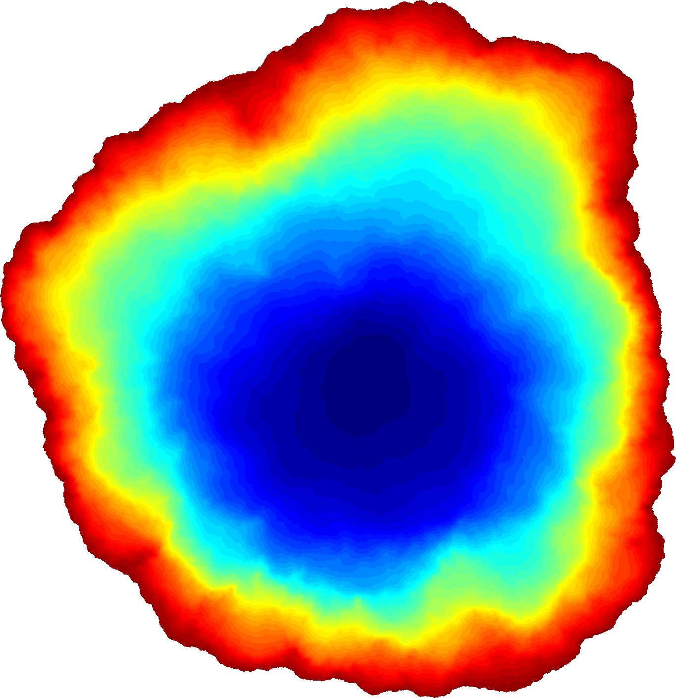
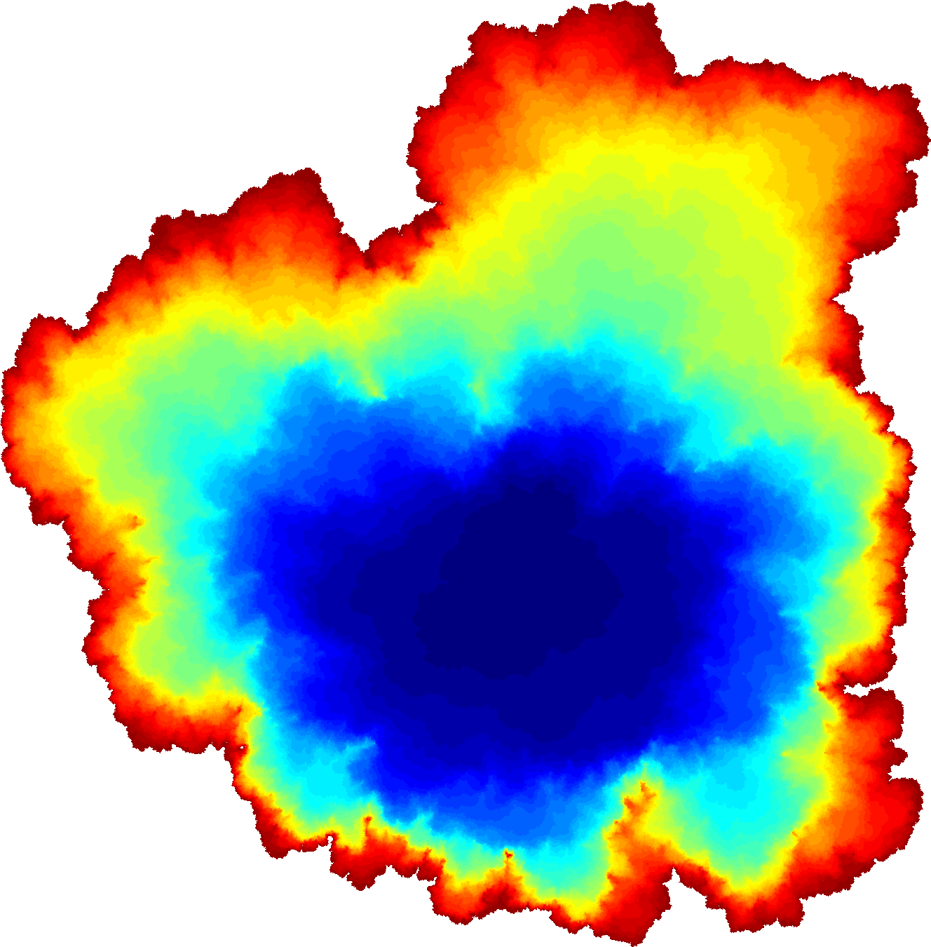
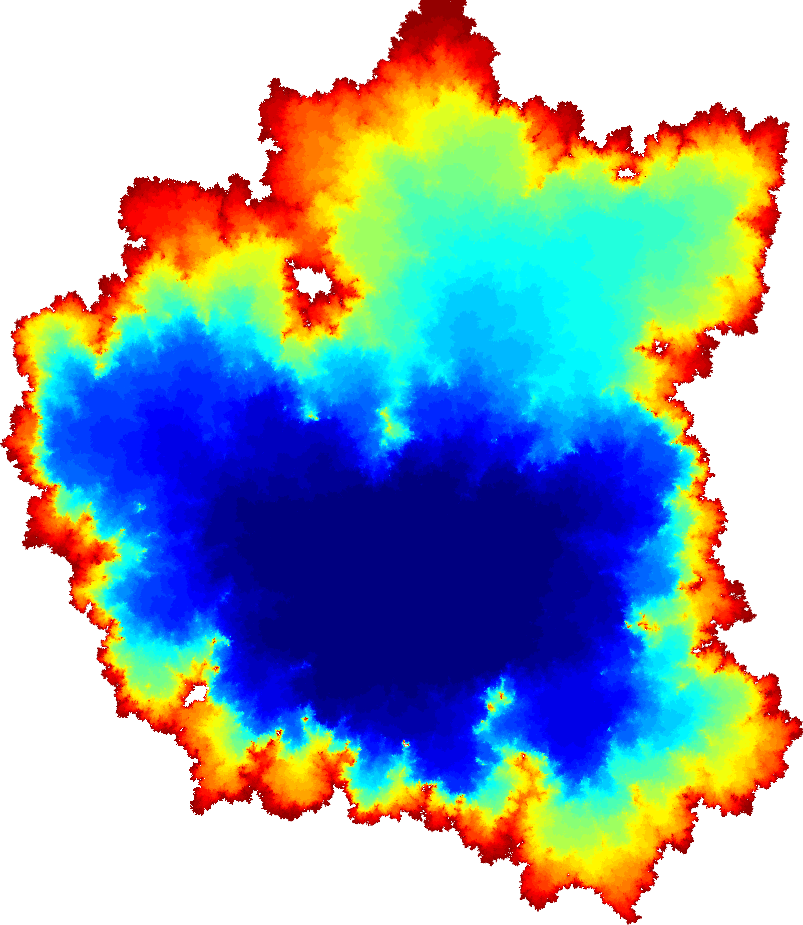
Figure 1. Simulations of $\gamma$-LQG harmonic balls with respect to the same GFF instance for $\gamma=0.5,1.0,1.8$. The colors distinguish harmonic balls of different mass. From the figures, it appears that the complement of an LQG harmonic ball is not necessarily connected. We expect that this is the case for a ‘typical’ LQG harmonic ball.

Let $\mu$ be a locally finite Radon measure on $\mathbb{C}$ . A harmonic ball for $\mu$ is an open set $\Lambda\subset\mathbb{C}$ containing the origin which satisfies the mean-value property

(1.1) $$f(0)=\frac{1}{\mu(\Lambda)}\int_{\Lambda}f(z)\mu(dz),$$

for all functions $f$ which are harmonic in a neighborhood of the closure of $\Lambda$.

1.1.1. Liouville quantum gravity

In this article, we will construct and study harmonic balls in the setting of Liouville quantum gravity (LQG). LQG is a canonical one-parameter family of random fractal surfaces which were introduced by Polyakov in the 1980s in the context of bosonic string theory [polyakov-qg1]. One sense in which these surfaces are canonical is that they are known or conjectured to describe the scaling limits of various types of random planar maps (see Section 1.3 for more details).

Heuristically, for $\gamma\in(0,2)$ and a domain $U\subset\mathbb{C}$, a $\gamma$-LQG surface parameterized by $U$ is the two-dimensional Riemannian manifold with Riemannian metric tensor $e^{\gamma h}\,(dx^{2}+dy^{2})$, where $dx^{2}+dy^{2}$ is the Euclidean metric tensor and $h$ is a variant of the Gaussian free field (GFF) on $U$. This metric tensor does not make literal sense since $h$ is a random generalized function, not a true function. Nevertheless, it is still possible to define the associated volume form, a.k.a. the $\gamma$-Liouville measure. This is a random, locally finite Radon measure on $U$ which is informally given by

(1.2) $$\mu_{h}(dz)=e^{\gamma h(z)}\,dz,$$

where $dz$ denotes Lebesgue measure.

The expression (1.2) can be made rigorous as part of a general theory of regularized random measures called Gaussian multiplicative chaos [kahane1985chaos, robert2010gaussian, rhodes2014gaussian]. This theory shows that the Liouville measure is a well-defined (random) Radon measure which is measurable with respect to $h$ (the converse is also true [berestycki2014equivalence]). However, the Liouville measure is quite irregular: $\mu_{h}$ is supported on the ‘thick’ points of the GFF, a dense fractal set of Hausdorff dimension $2-\frac{\gamma^{2}}{2}$, and hence is mutually singular with respect to Lebesgue measure [duplantier2011liouville, hu2010thick].

There is a vast literature on LQG: see [gwynne2020random, sheffield-icm] for introductory survey articles and [berestycki2021gaussian] for a more detailed introduction. However, only minimal prior knowledge of this literature is needed to read this paper. The necessary background will be reviewed in Section 2.

1.1.2. LQG harmonic balls

We will be interested in harmonic balls, as defined in (1.1), in the case when $\mu$ is the $\gamma$-Liouville measure, $\mu_{h}$, for some $\gamma\in(0,2)$. We call these domains $\gamma$-LQG harmonic balls. One of our main motivations for studying LQG harmonic balls is that we expect them to be the scaling limits of internal diffusion limited aggregation (IDLA) [lawler1992internal] on random planar maps. See Section 1.3 for further discussion.

We will construct $\gamma$-LQG harmonic balls via a certain partial differential equation involving $\mu_{h}$. In particular, this PDE, Hele-Shaw flow, describes the movement of viscous fluid on a $\gamma$-LQG surface, see, e.g., [roos2016partial]. The irregularity of $\mu_{h}$ precludes applying the classical theory of existence and uniqueness of harmonic balls [sakai1984solutions, friedman1988free, gustafsson1990onquadraturedomains, caffarelli1998obstacle] in the LQG setting. Much of the existing technology requires $\mu$ to be bounded from above and below by a multiple of the Lebesgue measure — a constraint too strict to be satisfied, even approximately, by $\mu_{h}$. Consequently, even the existence of $\gamma$-LQG harmonic balls is far from obvious. Indeed, nontrivial harmonic balls do not exist in general — take, for instance, $\mu$ to be Dirac measure supported away from the origin.

We address this difficulty by following a different path, inspired by arguments from discrete Laplacian growth [duminil2013containing, jerison2013internal]. Roughly speaking, we show that it is unlikely for Brownian motion to avoid regions of large $\mu_{h}$-mass and then use this to show harmonic balls exist. This argument also leads to geometric requirements harmonic balls satisfy. We later use these requirements to show that ‘typical’ $\gamma$-LQG harmonic balls are neither Lipschitz domains nor LQG metric balls.

In contrast to the constructions of other objects associated with LQG, such as the LQG measure, the LQG metric, and Liouville Brownian motion, our construction of LQG harmonic balls does not use any approximation or regularization procedure. Rather, LQG harmonic balls are constructed directly as the solutions of an optimization problem involving the LQG measure (see Section 3.1).

An LQG surface is a certain type of random fractal (albeit not one defined as a subset of $\mathbb{R}^{d}$ for some $d$). Analysis on fractals is a well-studied topic, see, e.g., [kigami2001analysis, strichartz2006differential, strichartz2020analysis]. One program of research in this area is to construct the Laplacian on a fractal and then use this to develop a theory of elliptic PDE on the fractal. As discussed further in Section 2, Brownian motion, and hence the Laplacian, has been constructed on LQG surfaces [garban2016liouville, berestycki2015diffusion]. The present paper may be thought of as an initial step in the study of PDE on LQG surfaces.

1.2. Statement of the main result

Fix the LQG parameter $\gamma\in(0,2)$. Let $h$ be a whole-plane Gaussian free field, or more generally a whole-plane Gaussian free field plus the function $-\boldsymbol{\alpha}_{0}\log|\cdot|$, where $\boldsymbol{\alpha}_{0}<Q:=2/\gamma+\gamma/2$. Let $\mu_{h}$ be the $\gamma$-LQG area measure associated with $h$. The precise definitions of $h$ and $\mu_{h}$ will be reviewed in Section 2. For now, the unfamiliar reader can think of $\mu_{h}$ as a random, non-atomic, locally finite Borel measure on $\mathbb{C}$ which assigns positive mass to every open subset of $\mathbb{C}$.

Our main result concerns existence and uniqueness of a family of $\gamma$-LQG harmonic balls. To prove uniqueness, we enlarge the class of harmonic functions in the definition to include those of the form,

(1.3) $$\tilde{H}_{O}(D)=\{\int_{O}G_{O}(\cdot,y)\,\nu(dy):\mbox{$\nu$ is a signed Radon measure with support in $O\backslash D$}\},$$

where $O,D\subset\mathbb{C}$ are bounded open sets and $G_{O}$ is the Green’s function for Brownian motion in the domain $O$ (defined in Section 2.3 below). That is, $\Lambda$ is a harmonic ball if (1.1) is satisfied for all functions $f=f_{1}+f_{2}$ where $f_{1}$ is harmonic in a neighborhood of the closure of $\Lambda$ and $f_{2}\in\tilde{H}_{O}(\Lambda)$ for some $O\Supset\Lambda$.

We are now ready to state our main existence and uniqueness result.

Theorem 1.1 (Existence and uniqueness of harmonic balls).

On an event of probability one, there exists a unique family of harmonic balls $\{\Lambda_{t}\}_{t>0}$ satisfying the following properties:

1. For each $t>0$, $\mu_{h}(\Lambda_{t})=t$, $\mu_{h}(\partial\Lambda_{t})=0$, and $\Lambda_{t}$ is equal to the interior of its closure.

2. The domains $\Lambda_{t}$ are bounded, connected, contain the origin, increase continuously in $t$ (in the Hausdorff topology), and satisfy $\cap_{t>0}\Lambda_{t}=\{0\}$.

In some literature on harmonic balls, e.g., [sakai1984solutions] or [hedenmalm2002hele], uniqueness is only proven up to sets of zero mass. In our setting, we get exact uniqueness thanks to the requirement that $\Lambda_{t}$ is equal to the interior of its closure.

We also show that typical harmonic balls are ‘novel’; that is, they are neither Euclidean balls nor LQG metric balls. We also show that the boundaries of their complementary connected components are Jordan curves. Compare Figures 1 and 2. The precise definition of the LQG metric ball will be given in Section 2; for now the reader may think of it as the natural notion of metric ball on an LQG surface.

Theorem 1.2 (Novelty of harmonic balls).

The following is true on an event of probability 1. For Lebesgue-a.e. t, $\Lambda_{t}$, constructed in Theorem 1.1, is neither a Lipschitz domain nor an LQG-metric ball. Moreover, for each $t>0$ the boundaries of the connected components of $\mathbb{C}\setminus\overline{\Lambda}_{t}$ are Jordan curves.

We remark that the harmonic balls given by Theorem 1.1 are locally determined by $\mu_{h}$, in the sense of the following statement.

Proposition 1.3.

For each fixed $t\geq 0$, the closed LQG harmonic ball $\overline{\Lambda}_{t}$ is a local set for $h$ in the sense of [ss-contour, Lemma 3.9], i.e., for each deterministic open set $U\subset\mathbb{C}$, the event $\{\overline{\Lambda}_{t}\subset U\}$ is measurable with respect to $\sigma(h|_{U})$.

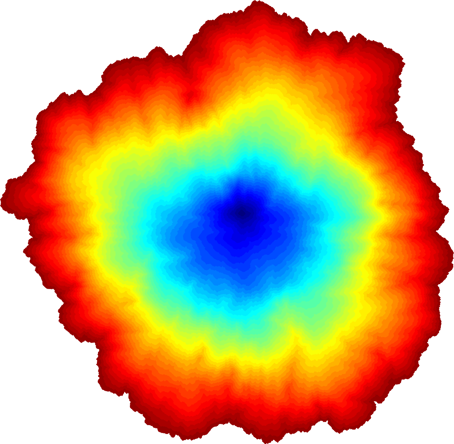
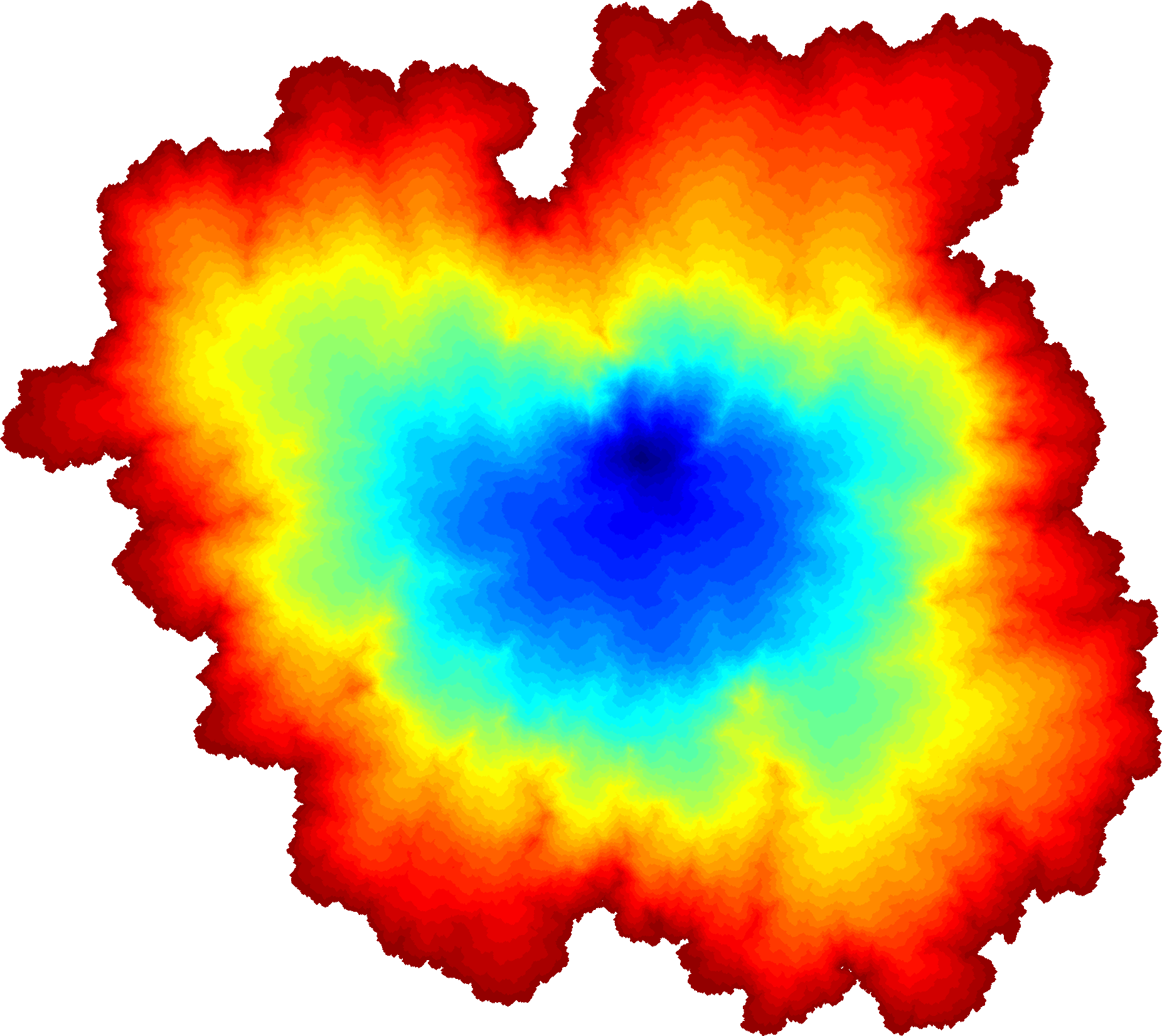
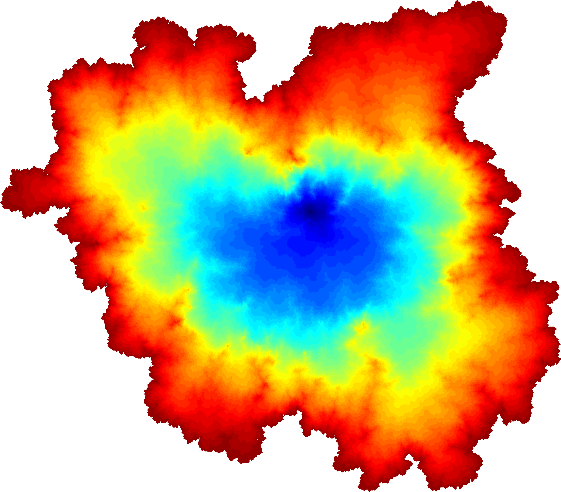
Figure 2. Simulations of $\gamma$-LQG metric balls with respect to the same GFF instance as Figure 1 for $\gamma=0.5,1.0,1.8$.

1.3. Background

We provide some context and motivation for the study of harmonic balls on LQG surfaces.

1.3.1. Harmonic balls

The term ‘harmonic ball’ was coined by Shahgholian-Sjödin in [shahgholian2013harmonic] and is a special case of quadrature domains for harmonic functions. A quadrature domain is a subset of $\mathbb{C}$ for which the integral of a harmonic function can be expressed as a sum of simpler functionals (such as point evaluations). Quadrature domains have a long history and are closely related to classical balayage (sweeping) [doob1984classical], Hele-Shaw flow [gustafsson2006conformal], obstacle problems [sakai1984solutions], and Laplacian growth [zidarov1990inverse, levine2017laplacian]. We direct the interested reader to [gustafsson2005quadrature, gustafsson2004lectures] and the introductions of the theses of Roos [roos2016partial] and Sjödin [sjodin2005topics] for excellent expositions.

Of particular relevance to our work are the papers of Hedenmalm-Shimorin [hedenmalm2002hele] and Gustafsson-Roos [gustafsson2018partial] which construct and analyze harmonic balls on Riemannian manifolds. Hedenmalm-Shimorin, building upon the work of Sakai [sakai1991regularity], show that harmonic balls on sufficiently smooth hyperbolic surfaces have boundaries which are the unions of a finite number of real analytic simple curves. Gustafsson-Roos show that harmonic balls and geodesic balls coincide on Riemannian surfaces if and only if the Gaussian curvature of the manifold is constant. We emphasize that while some of the basic constructions in these works may be adapted to our setting, an LQG surface is not a Riemannian manifold in the literal sense and so the results do not apply.

1.3.2. Internal DLA

One of our main motivations for studying LQG harmonic balls stems from a connection with internal diffusion limited aggregation (IDLA) on random planar maps. IDLA was introduced as a toy model for chemical corrosion in [meakin1986formation] and is a special case of a growth model studied by Diaconis-Fulton in [diaconis1991growth]. IDLA is a random aggregation model defined as follows: start with $n$ walkers at the origin in $\mathbb{Z}^{2}$ and let each walker evolve according to a simple random walk until it reach a site in $\mathbb{Z}^{2}$ not occupied by any previous walker. This rule generates a growing sequence of sets $A_{n}\subset\mathbb{Z}^{2}$ indexed by the number of walkers $n\in\mathbb{N}$.

In a foundational work, Lawler-Bramson-Griffeath proved that $A_{n}$, suitably rescaled, converges to a Euclidean ball in $\mathbb{R}^{2}$ as $n$ goes to infinity [lawler1992internal, lawler1995subdiffusive]. Later, Asselah-Gaudillère [asselah2013logarithmic, asselah2013sublogarithmic] and independently Jerison-Levine-Sheffield established logarithmic fluctuations of $A_{n}$ around its limit [jerison2012logarithmic, jerison2013internal, jerison2014internal].

Implicit in the proof of Lawler-Bramson-Griffeath is that harmonic balls are Euclidean balls when $\mu$ is the Lebesgue measure — a simple proof of this was given by Ülkü Kuran in 1972 [kuran1972mean]. Interestingly, the connection between IDLA and quadrature domains generalizes. Levine-Peres showed in [levine2010scaling] that the scaling limit of IDLA for any initial condition (for example multiple point sources) is given by a corresponding quadrature domain.

IDLA has also been studied on several other graphs including: Cayley graphs of groups with polynomial [blachere2001internal] and exponential [blachere2007internal, huss2008internal] growth, supercritical percolation clusters [shellef2010idla, duminil2013containing], Sierpinski gasket graphs [chen2017internal], and cylinders [jerison2014chapter, levine2019long, silvestri2020internal]— see [sava2021fractals] for a thorough survey of IDLA. In each of these cases the limit shape is either a Euclidean ball or a metric ball. On the other hand, Asselah-Rahmani showed that IDLA on the comb lattice has a limit shape which is neither a Euclidean ball nor a metric ball but rather a domain which satisfies a certain mean-value property [asselah2016fluctuations] (see also [huss-sava-comb]). In a similar vein, Lucas has shown that IDLA with biased random walkers on $\mathbb{Z}^{d}$ converges under parabolic scaling to a domain which satisfies the mean-value property for caloric functions [lucas2014limiting].

1.3.3. Random planar maps

A planar map is a graph embedded in $\mathbb{C}$ in such a way that no two edges cross, viewed modulo orientation preserving homeomorphisms $\mathbb{C}\rightarrow\mathbb{C}$. Various types of random planar maps are expected, and in some cases proven, to converge to $\gamma$-LQG surfaces. For example, uniform random planar maps (including uniform triangulations, quadrangulations, etc.) converge to $\sqrt{8/3}$-LQG surfaces in the Gromov-Hausdorff sense [legall-uniqueness, miermont-brownian-map, lqg-tbm1, lqg-tbm2] and, at least in the case of triangulations, when embedded into $\mathbb{C}$ via the so-called Cardy embedding [hs-cardy-embedding]. Similar convergence results are expected to hold for various types of non-uniform random planar maps toward $\gamma$-LQG with $\gamma\not=\sqrt{8/3}$. For example, random planar maps sampled with probability proportional to the number of spanning trees they admit are expected to converge to $\sqrt{2}$-LQG. We refer to [ghs-mating-survey] for a survey of work relating random planar maps and LQG.

The aforementioned results on IDLA suggest that the scaling limits of IDLA on random planar maps are described by harmonic balls on LQG surfaces. Random walks on (reasonably embedded) random planar maps are also expected to converge to (time changes of) Brownian motions on LQG surfaces — this has recently been proven for a one-parameter family of random planar maps called mated-CRT maps in [gms-tutte, berestycki2020random]. In a companion work [bou2022idla], we verify that the scaling limit of IDLA on mated-CRT maps is given by LQG harmonic balls. It is still an open problem to prove this for other random planar map models, e.g., uniform random planar maps (see Problem 1).

1.4. Open problems

We collect some questions suggested by this work. The first has been mentioned previously and is arguably the most important question here.

Problem 1.

Show that the scaling limit of IDLA on random planar maps in the appropriate $\gamma$-LQG universality class, other than mated-CRT maps, is described by $\gamma$-LQG harmonic balls. For example, on a uniform planar map show that the scaling limit of IDLA is a $\sqrt{8/3}$-LQG harmonic ball.

Possible topologies of convergence in Problem 1 include a version of the Gromov-Hausdorff distance for metric spaces decorated by compact sets; or convergence of the IDLA clusters w.r.t. the Hausdorff distance when the random planar map is embedded into $\mathbb{C}$ appropriately. There are also some purely continuum directions one could pursue — the following is an example.

Problem 2.

Compute the Hausdorff dimension of the boundary of an LQG harmonic ball, with respect to the Euclidean metric and with respect to the LQG metric.

We expect that the Euclidean and LQG dimensions of the harmonic ball boundary are each strictly greater than one. We note that the Hausdorff dimensions of the boundary of an LQG metric ball with respect to the Euclidean and LQG metrics have been computed in [gwynne-dimension-metric-ball, MR4408506].

It is also of interest to determine the analogue of LQG metric geodesics in the setting of harmonic balls. In particular, we are interested in extending the theory of ‘Hele-Shaw geodesics’, in the sense of [hedenmalm2002hele], to our setting. As mentioned previously, Hedenmalm-Shimorin in [hedenmalm2002hele] investigated harmonic balls on smooth Riemannian surfaces and showed that their boundaries are piece-wise smooth curves. Because of this smoothness, they were able to define Hele-Shaw geodesics as a family of curves originating from a fixed point which are orthogonal to the boundary of a harmonic ball at any point. One may think of these geodesics as describing the trajectory of a single fluid particle started at a fixed point on a Riemannian surface. As LQG harmonic balls do not have smooth boundaries, it is unclear how to adapt this to our setting, but a weaker version of these objects may exist.

Problem 3.

Construct and analyze the analogue of ‘Hele-Shaw geodesics’ [hedenmalm2002hele] on LQG surfaces.

A helpful intermediate step would be to show some additional regularity of harmonic balls. For example, the harmonic balls we construct are monotone in $t$ but we are unable to show strict monotonicity in $t$.

Problem 4.

Prove or disprove that the family of harmonic balls $\{\Lambda_{t}\}_{t>0}$, given by Theorem 1.1, is strictly monotone in $t$, i.e., $\overline{\Lambda}_{s}\subset\Lambda_{t}$ whenever $s<t$.

1.5. Paper and proof outline

We start in Section 2 by reviewing the definition of the GFF, the definition of LQG, and some results about Liouville Brownian motion. We then introduce the fundamental obstacle problem which we use to construct candidate harmonic balls, clusters, in Section 3 and establish some basic properties of the constructed clusters in Section 4. The results of Sections 3 and 4 are straightforward extensions of those appearing in the obstacle problem literature — the only property of the LQG measure which is used there is that it is a Radon measure with certain volume growth bounds, Lemma 2.4 below.

Several of the results of Sections 3 and 4 (including the statement that the clusters are harmonic balls, see Section LABEL:subsec:subharmonic) are conditional on two properties which are not proven in these sections: namely, that the clusters do not attain a large Euclidean diameter in an arbitrarily small amount of time and that the boundaries of the clusters have zero LQG mass. Establishing these properties is the main goal of Sections LABEL:sec:non-degenerate through LABEL:sec:boundary-measure-zero.

In Section LABEL:sec:non-degenerate we outline a strategy for showing that the clusters are harmonic balls; that is, they grow continuously and their boundaries have zero LQG mass. Our approach for verifying these properties is completely new and relies on a novel Harnack-type estimate, Proposition LABEL:prop:harnack-type-property, which clusters must satisfy. In particular, this estimate forces clusters to have ‘no thin-tentacles’, as in [jerison2013internal]. Roughly speaking, our Harnack-type estimate says that there is a constant $\alpha>0$ such that if $A\subset\mathbb{C}$ is an annulus on which the LQG measure $\mu_{h}$ is reasonably well-behaved, then if the cluster $\Lambda_{t}$ crosses between the inner and outer boundaries of $A$ we must have $\mu_{h}(A\cap\Lambda_{t})\geq\alpha\mu_{h}(A)$. Our proof of the Harnack-type estimate in Section LABEL:sec:harnack-type-estimate combines potential theoretic techniques with methods from LQG theory. See the beginning of Section LABEL:sec:harnack-type-estimate for an outline of the argument.

In Sections LABEL:sec:upper-bound and LABEL:sec:boundary-measure-zero, respectively, we use the Harnack-type estimate to prove that the clusters grow continuously in time, Proposition LABEL:prop:continuity-of-clusters, and that boundaries of the clusters have measure zero, Proposition LABEL:prop:boundary-measure-zero. As demonstrated in Theorem LABEL:theorem:full-theorem-minus-uniqueness, these properties are enough to ensure that clusters are LQG harmonic balls.

Having constructed LQG harmonic balls, we show, by adapting ideas from the obstacle problem literature [sakai2006quadrature], their uniqueness, Proposition LABEL:prop:uniqueness, in Section LABEL:sec:uniqueness.

The Harnack-type estimate imposes strong geometric constraints on LQG harmonic balls. For instance, it disallows LQG harmonic balls from ‘crossing’ annuli too many times, Lemma LABEL:lemma:cannot-cross. We use this in Section LABEL:sec:boundary-curves to show that the boundaries of complementary connected components of LQG harmonic balls are Jordan curves, Proposition LABEL:prop:boundary-simple-loop.

These geometric constraints may also be translated into a strong relationship between LQG harmonic balls and the underlying LQG area measure, Lemma LABEL:lemma:harmonic-comparison-chain. Since the LQG measure is quite variable, this imposes an irregularity on LQG harmonic balls. We use this to show that LQG harmonic balls do not satisfy the cone condition, Lemma LABEL:lemma:no-exterior-cone-condition, in Section LABEL:subsec:not-lipschitz. Consequently, LQG harmonic balls cannot be Lipschitz domains.

Another feature of the Harnack-type estimate is that it precludes LQG harmonic balls from having ‘approximate pinch points’ which have small Euclidean diameter but which come close to disconnecting sets of large LQG mass from the origin within the cluster. On the other hand, an LQG metric ball has such approximate pinch points, as we show in Section LABEL:subsec:not-lqg-metric-ball. This shows that LQG harmonic balls are not LQG metric balls. A key technical input in the proof is Proposition LABEL:prop:mass-diam-gen, which shows that a region in the plane can have small LQG diameter but large LQG mass simultaneously with positive probability.

1.6. Notation and conventions

• Inequalities/equalities between functions/scalars are interpreted pointwise.

• Differential inequalities/equalities are interpreted in the distributional sense.

• For a set $A\subset\mathbb{C}$, $\partial A$ denotes its topological boundary, $\overline{A}=A\cup\partial A$ its closure, and $\mathrm{int}(A)$ its interior.

• For two sets $A,B\subset\mathbb{C}$, say that $A\Subset B$ if $\overline{A}\subset B$.

• $B_{r}(x)$ denotes the open ball of Euclidean radius $r>0$ centered at $x\in\mathbb{C}$, when $x$ is omitted, the ball is centered at 0.

• For a set $A\subset\mathbb{C}$, we denote the $r$-neighborhood of $A$ by $B_{r}(A)=A+B_{r}$.

• For $0<r_{1}<r_{2}$, denote an open annulus centered at $z$ by

  (1.4) $$\mathbb{A}_{r_{1},r_{2}}(z)=B_{r_{2}}(z)\backslash\overline{B}_{r_{1}}(z)$$

  and $\mathbb{A}_{r_{1},r_{2}}:=\mathbb{A}_{r_{1},r_{2}}(0)$.

• Let $\{E^{r}\}_{r>0}$ be a one-parameter family of events. We say that $E^{r}$ occurs with polynomially high probability as $r\to 0$ if there exists $p>0$ such that $\mathbb{P}[E^{r}]\geq 1-O(r^{p})$.

• For two sets $A,B\subset\mathbb{C}$, $\mathop{\bf dist{}}(A,B)=\inf_{a\in A,b\in B}\mathop{\bf dist{}}(a,b)$ where $\mathop{\bf dist{}}$ denotes the Euclidean distance between two points.

Acknowledgments

A.B. thanks Charlie Smart and Bill Cooperman for useful discussions. A.B. was partially supported by NSF grant DMS-2202940 and a Stevanovich fellowship. E.G. was partially supported by a Clay research fellowship.

2. Preliminaries

In this section we review the definitions and basic properties of the Gaussian Free Field (GFF), the Liouville Quantum Gravity (LQG) area measure, and the LQG metric. We present just enough exposition for the purposes of this paper; the book [berestycki2021gaussian] and surveys [gwynne2020random, ding2021introduction, sheffield-icm] provide more details.

2.1. Gaussian free field

The whole-plane GFF $h^{\mathbb{C}}$ is the centered Gaussian random generalized function on $\mathbb{C}$ with covariances

(2.1) $$\mathop{\bf Cov{}}(h^{\mathbb{C}}(z),h^{\mathbb{C}}(w)):=\log\frac{\max(|z|,1)\max(|w|,1)}{|z-w|},\quad\forall z,w\in\mathbb{C}.$$

The GFF $h^{\mathbb{C}}$ is not well-defined pointwise since the covariance kernel in (2.1) diverges to $\infty$ as $z\to w$. Nevertheless, for $z\in\mathbb{C}$ and $r>0$, one can define the average of $h^{\mathbb{C}}$ over the circle of radius $r$ centered at $z$, which we denote by $h^{\mathbb{C}}_{r}(z)$ [duplantier2011liouville, Section 3.1].

The whole plane GFF is usually defined modulo additive constant. Our choice of covariance in (2.1) corresponds to fixing this additive constant so that $h^{\mathbb{C}}_{1}(0)=0$ (see, e.g., [vargas2017lecture, Section 2.1.1]).

The law of the whole-plane GFF, viewed modulo additive constant, is invariant under complex affine transformations of $\mathbb{C}$. This translates into the following invariance property for $h^{\mathbb{C}}$,

(2.2) $$h^{\mathbb{C}}\overset{d}{=}h^{\mathbb{C}}(a\cdot+b)-h^{\mathbb{C}}_{|a|}(b),\quad\forall a\in\mathbb{C}\backslash\{0\},\quad\forall b\in\mathbb{C}.$$

Fix $\gamma\in(0,2)$ and $\boldsymbol{\alpha}_{0}\in(-\infty,Q)$, where

(2.3) $$Q:=\frac{2}{\gamma}+\frac{\gamma}{2}.$$

Throughout this paper we take $h$ to be the whole-plane GFF with an $\boldsymbol{\alpha}_{0}$ log singularity at the origin.

Specifically, let $h^{\mathbb{C}}$ denote the whole-plane GFF normalized so that its circle average over the unit disk is zero and set

(2.4) $$h=h^{\mathbb{C}}-\boldsymbol{\alpha}_{0}\log|\cdot|.$$

It is immediate from (2.2) that

(2.5) $$h\overset{d}{=}h(a\cdot)-h_{|a|},\quad\forall a\in\mathbb{C}\backslash\{0\}.$$

2.2. Liouville Quantum Gravity

Let $\mu_{h}$ denote the $\gamma$-LQG area (Liouville) measure associated to $h$. One of the (many) possible ways of defining $\mu_{h}$ is as the a.s. weak limit

(2.6) $$\mu_{h}=\lim_{\epsilon\rightarrow 0}\epsilon^{\gamma^{2}/2}e^{\gamma h_{\epsilon}(z)}\,dz$$

where $dz$ denotes Lebesgue measure and $h_{\epsilon}(z)$ is the circle average [duplantier2011liouville, sheffield2016field]. In fact, the measure $\mu_{\tilde{h}}$ exists for any random generalized function $\tilde{h}$ of the form $h+f$ where $f$ is a possibly random continuous function.

Fact 2.1 (LQG measure).

The LQG area measure $\mu_{h}$ satisfies the following properties.

1. Radon measure. A.s., $\mu_{h}$ is a non-atomic Radon measure.

2. Locality. For every deterministic open set $U\subset\mathbb{C}$, $\mu_{h}(U)$ is given by a measurable function of $h|_{U}$.

3. Weyl scaling. A.s., $e^{\gamma f}\cdot\mu_{h}=\mu_{h+f}$ for every continuous function $f:\mathbb{C}\to\mathbb{R}$.

4. Conformal covariance. A.s., the following is true. Let $U,\tilde{U}\subset\mathbb{C}$ be open and let $\phi$ be a conformal map from $\tilde{U}$ to $U$. Then, with $Q$ as in (2.3),

   (2.7) $$\mu_{h\circ\phi+Q\log|\phi^{\prime}|}(A)=\mu_{h}(\phi(A))\quad\mbox{for all Borel measurable $A\subset\tilde{U}$}.$$

The first three properties in Fact 2.1 are immediate from the definition (2.6). The conformal covariance property was proven to hold a.s. for a fixed conformal map in [duplantier2011liouville, Proposition 2.1] and extended to all conformal maps simultaneously in [sheffield2016field].

It was shown in [ding2020tightness, gwynne2021existence] that one can define also the LQG metric $D_{h}$, which is the limit of regularized versions of the Riemannian distance function associated with the Riemannian metric tensor $e^{\gamma h}(dx^{2}+dy^{2})$. Like the LQG measure, the LQG metric is a fractal-type object. It induces the same topology on $\mathbb{C}$ as the Euclidean metric, but the Hausdorff dimension of the metric space $(\mathbb{C},D_{h})$ is a.s. given by a deterministic number $d_{\gamma}>2$ [gp-kpz, Corollary 1.7]. The value of $d_{\gamma}$ is not known explicitly except that $d_{\sqrt{8/3}}=4$.

In order to state an analog of Fact 2.1 for the LQG metric, we make the following definitions. For a Euclidean-continuous path $P$ in $\mathbb{C}$, we write $\mathrm{len}(P;D_{h})$ for its length with respect to $D_{h}$. For an open set $U\subset\mathbb{C}$, the internal metric of $D_{h}$ on $U$ is defined by

(2.8) $$D_{h}(z,w;U)=\inf\{\mathrm{len}(P;D_{h}):\mbox{$P$ is a path from $z$ to $w$ in $U$}\},\quad\mbox{$\forall z,w,\in U$}.$$

As in the case of the measure, the metric $D_{\tilde{h}}$ exists whenever $\tilde{h}=h+f$, where $f$ is a possibly random continuous function.

Fact 2.2 (LQG metric).

The LQG metric $D_{h}$ has the following properties.

1. Euclidean topology and length metric. A.s., $D_{h}$ induces the same topology on $\mathbb{C}$ as the Euclidean metric and is a length metric, that is, $D_{h}(z,w)$ is the infimum of the $D_{h}$-length of paths from $z$ to $w$.

2. Locality. For every deterministic open set $U\subset\mathbb{C}$, the $D_{h}$-internal metric on $U$ is given by a measurable function of $h|_{U}$.

3. Weyl scaling. Let

   (2.9) $$\xi=\frac{\gamma}{d_{\gamma}},$$

   where $d_{\gamma}$ is the Hausdorff dimension of the $\gamma$-LQG metric as above. Almost surely, for every continuous function $f:\mathbb{C}\to\mathbb{R}$,

   $$D_{h+f}(u,v)=\inf_{P:u\to v}\int_{0}^{\mathrm{len}(P;D_{h})}e^{\xi f(P(t))}dt,\quad\forall u,v\in\mathbb{C}.$$

4. Coordinate change for scaling and translation. Let $r>0$ and $z\in C$. Almost surely, with $Q$ as in (2.3),

   $$D_{h}(ru+z,rv+z)=D_{h(r\cdot+z)+Q\log r}(u,v),\quad\forall u,v,\in C.$$

The properties listed in Fact 2.2 were verified for the LQG metric in [ding2020tightness, dubedat2020weak, gwynne2021existence]. In fact, it is shown in [gwynne2021existence] that these properties uniquely characterize $D_{h}$.

In what follows, for sets $A,B\subset\mathbb{C}$, we write

(2.10) $$D_{h}(A,B)=\inf_{x\in A,y\in B}D_{h}(x,y).$$

For disjoint compact sets $K_{1},K_{2}\subset\mathbb{C}$, a $D_{h}$-geodesic from $K_{1}$ to $K_{2}$ is a path from $K_{1}$ to $K_{2}$ of minimal $D_{h}$-length. It is easily seen from the length metric property and a compactness argument that $D_{h}$-geodesics always exist (see, e.g., [bbi-metric-geometry, Corollary 2.5.20]).

2.3. Green’s function

Let $G_{O}:\overline{O}\times\overline{O}\to\mathbb{R}\cup\{\infty\}$ denote the Green’s function for standard Brownian motion killed upon exiting a bounded open set $O\subset\mathbb{C}$. We make use of the following standard properties of the Green’s function of a (sufficiently nice) set.

Proposition 2.3.

The Green’s function of a ball, $B_{R}$ of radius $R>0$, has the following properties for every $x\in B_{R}$.

• Fundamental solution: $\Delta G_{B_{R}}(x,\cdot)=-\delta_{x}(\cdot)$ on $B_{R}$.

• Positive: $G_{B_{R}}(x,\cdot)>0$ on $B_{R}$.

• Zero boundary: $G_{B_{R}}(x,\cdot)=0$ on $\partial B_{R}$.

• Smooth away from the pole: $G_{B_{R}}(x,\cdot)$ is infinitely differentiable away from $x$.

2.4. Liouville Potential Theory

In this section we collect well known potential theoretic estimates on the LQG measure. We first note bounds on the LQG mass of annuli and balls.

Lemma 2.4.

For each $\beta^{+}\in(0,(2-\gamma)^{2}/2)$ and $\beta^{-}>(2+\gamma)^{2}/2$ it holds with polynomially high probability as $\epsilon\to 0$ that

(2.11) $$\epsilon^{\beta^{-}}\leq\mu_{h}(B_{\epsilon}(z))\leq\epsilon^{\beta^{+}},\quad\forall z\in B_{1}.$$

Furthermore, for each $0<r_{1}<r_{2}$ there exists constants $C_{1},C_{2}$ so that for all $z\in B_{1}$

(2.12) $$C_{2}\epsilon^{\beta^{-}}\leq\mu_{h}(\mathbb{A}_{r_{1}\epsilon,r_{2}\epsilon}(z))\leq C_{1}\epsilon^{\beta^{+}}$$

with polynomially high probability as $\epsilon\to 0$, where here we use the notation for annuli from (1.4).

Proof.

Exactly the same argument as in [berestycki2020random, Lemma A.1] shows that (2.11) holds with polynomially high probability as $\epsilon\to 0$. The estimate (2.12) follows from (2.11) and the fact that

$$B_{\frac{r_{2}-r_{1}}{4}\epsilon}(z+\frac{r_{2}\epsilon+r_{1}\epsilon}{2}e_{1})\subset\mathbb{A}_{r_{1}\epsilon,r_{2}\epsilon}(z)\subset B_{r_{2}\epsilon}(z)$$

where $e_{1}=(1,0)$. ∎

Liouville Brownian motion (LBM) is the natural diffusion associated with $\gamma$-LQG. Roughly speaking, LBM is obtained from ordinary Brownian motion (sampled independently from $h$) by changing time so that the process has ‘constant $\gamma$-LQG speed’. LBM was constructed in [berestycki2015diffusion, garban2016liouville]. It was shown in [berestycki2020random] to describe the scaling limit of random walk on a certain family of random planar maps.

The volume growth bounds given by Lemma 2.4 lead to control on the expected exit time of LBM from balls.

Proposition 2.5.

Let $O$ denote a smooth bounded open set. The expected exit time of LBM from $O$ started at $x\in O$ is finite and Hölder continuous in $x$. More generally, any $q$ of the form,

$$q(x)=\int_{O}G_{O}(x,y)f(y)d\mu_{h}(y)\qquad\mbox{for some $f\in L^{\infty}(\overline{O})$}$$

is finite and Hölder continuous in $\overline{O}$.

Proof.

Finiteness follows immediately from Lemma 2.4. Hölder continuity uses the embedding of Campanato spaces into Hölder spaces together with Lemma 2.4. See, for example, Section 16.2 (or the remark after Proposition 13.5) in [ponce2016elliptic]. ∎

The bounds also lead to continuity of the LBM heat kernel using the main result of [kigami2019]. Continuity of the LBM heat kernel (for other versions of the GFF) was previously established by [andres2016continuity] and [maillard2016liouville].

Let $K$ be a square in $\mathbb{C}$ and for $x\in\mathbb{C}$ let $\{\mathcal{B}_{t}^{x}\}_{t>0}$ denote $\gamma$-LBM with respect to the field $h$ started from $x$ with Neumann (reflecting) boundary conditions on $K$. The heat kernel $p^{K}_{t}$ of reflected LBM in $K$ is the function $p^{K}_{t}(x,y):(0,\infty)\times K\times K\to[0,\infty)$ such that

(2.13) $$\mathbb{P}[\mathcal{B}_{t}^{x}\in dy|h]=p^{K}_{t}(x,y)dy.$$

Proposition 2.6.

Let $K$ be a square in $\mathbb{C}$. Almost surely, the heat kernel $p^{K}_{t}(x,y)$ associated to $\gamma$-LBM with Neumann boundary conditions on $K$ exists, is finite, jointly continuous, and strictly positive for all $(t,x,y)\in(0,\infty)\times K\times K$.

Proof.

This is [kigami2019, Theorem 13.1] with input given by Lemma 2.4. Strictly speaking, [kigami2019, Theorem 13.1] concerns the transition density of reflecting $\gamma$-LBM in the unit square. A scaling argument shows that [kigami2019, Theorem 13.1] applies to the transition density of reflecting $\gamma$-LBM in any fixed square. ∎

3. Construction of harmonic balls via Hele-Shaw flow

In this section we construct domains which we will later show are $\gamma$-LQG harmonic balls. Specifically, we construct a family of sets $\{{\hyperref@@ii[eq:non-co-set]{\mathit{\Lambda}_{t}}}\}_{t>0}$ via an obstacle problem involving the Green’s function for the ball. This family describes the (restricted) flow of a viscous fluid injected onto an LQG surface. For the precise relationship between the obstacle problem and this flow, Hele-Shaw flow, see, for example, Chapter 3 of [gustafsson2006conformal]. Our construction is a standard one, see, e.g., [gustafsson1990onquadraturedomains, hedenmalm2002hele, shahgholian2013harmonic] and originates from the work of Sakai [sakai1984solutions].

In subsequent sections we show the existence of $T>0$ so that $\{{\hyperref@@ii[eq:non-co-set]{\mathit{\Lambda}_{t}}}\}_{0<t<T}$ are a family of harmonic balls satisfying the conditions in Theorem 1.1. We then use scale invariance and compatibility to extend this construction to all $t>0$.

3.1. Definition of the obstacle problem

We construct candidate harmonic balls via a technique similar to the Perron method involving the measure $\mu_{h}$ and the Green’s function for the ball. For each $t>0$ and ball $B_{r}$ the set of supersolutions is

(3.1) $$\hyperref@@ii[eq:super-solutions]{\mathcal{S}^{B_{r}}_{t}}=\{w\in C(\overline{B_{r}}):\Delta w\leq\mu_{h}\mbox{ in $B_{r}$}\mbox{ and }w\geq-tG_{B_{r}}(0,\cdot)\mbox{ in $\overline{B_{r}}$}\},$$

where $C(\overline{B_{r}})$ denotes the set of continuous functions on the closed ball. The least supersolution is defined as the pointwise infimum of all functions in SBrt,

(3.2) $$\hyperref@@ii[eq:least-super-solution]{w^{B_{r}}_{t}}=\inf\{w\in\hyperref@@ii[eq:super-solutions]{\mathcal{S}^{B_{r}}_{t}}\}$$

and the cluster as

(3.3) $$\hyperref@@ii[eq:non-co-set]{\mathit{\Lambda}^{B_{r}}_{t}}=\{x\in B_{r}:\hyperref@@ii[eq:least-super-solution]{w^{B_{r}}_{t}}(x)>-tG_{B_{r}}(0,x)\}.$$

We also consider the odometer

(3.4) $$\hyperref@@ii[eq:limit-odometer]{v^{B_{r}}_{t}}=\hyperref@@ii[eq:least-super-solution]{w^{B_{r}}_{t}}+tG_{B_{r}}(0,\cdot).$$

Note that SBrt is non-empty as it contains the zero function — thus wBrt always exists. This equation in (3.1) is known as an obstacle problem with obstacle given by the Green’s function. When $B_{r}$ is the unit ball (which for most of the paper will be the case), the distinguishing superscripts are omitted.

We think of the above obstacle problem as modeling the flow of liquid on a rough surface. A mass $t$ of fluid is injected into the origin and its growth is dictated by the infinitesimal capacity of the surface, namely, the measure $\mu_{h}$. The cluster Λt represents the settled fluid and vt captures the ‘work’ needed to spread the fluid.

From this physical picture, one expects that if $t$ is larger than $\mu_{h}(B_{r})$, then Λt should fill the entire ball. Moreover, if $\mu_{h}$ is regular enough, then for $t$ small the clusters should be strictly contained in $B_{r}$. Further, clusters with closures which do not intersect their boundaries should be compatible with clusters on smaller domains. We provide rigorous statements of these heuristics below.

3.2. Basic properties of the obstacle problem

We assert existence and basic regularity of solutions to the obstacle problem. These results are standard but for completeness are proved in Appendix LABEL:sec:obstacle-appendix. Each of the statements below made for $B_{1}$ also hold for each fixed $B_{r}$ for any $r>0$.

We first note that the least supersolution is indeed a supersolution.

Lemma 3.1.

On an event of probability 1, for all $t>0$, wt is finite, continuous, and an element of St.

The next lemma is a consequence of being the least supersolution.

Lemma 3.2.

On an event of probability 1, for all $t>0$, the cluster Λt is open and connected and

$$\Delta\hyperref@@ii[eq:least-super-solution]{w_{t}}=\mu_{h}|_{{{\hyperref@@ii[eq:non-co-set]{\mathit{\Lambda}_{t}}}}}+\nu|_{\partial{\hyperref@@ii[eq:non-co-set]{\mathit{\Lambda}_{t}}}}\quad\mbox{on $B_{1}$},$$

where $\nu$ is a Radon measure which is absolutely continuous with respect to $\mu_{h}$ and satisfies $0\leq\nu\leq\mu_{h}$. In particular,

$$\Delta\hyperref@@ii[eq:limit-odometer]{v_{t}}=-t\delta_{0}+\mu_{h}|_{{{\hyperref@@ii[eq:non-co-set]{\mathit{\Lambda}_{t}}}}}+\nu|_{\partial{\hyperref@@ii[eq:non-co-set]{\mathit{\Lambda}_{t}}}}\quad\mbox{on $B_{1}$}.$$

We will eventually show that a.s. $\mu_{h}(\partial{\hyperref@@ii[eq:non-co-set]{\mathit{\Lambda}_{t}}})=0$ for each $t>0$, which implies that $\nu=0$. However, for the time being we need to allow for the possibility that there is some mass on $\partial{\hyperref@@ii[eq:non-co-set]{\mathit{\Lambda}_{t}}}$.

We also have monotonicity of the clusters in $t$.

Lemma 3.3.

On an event of probability 1, for all $t_{1}\leq t_{2}$, $\hyperref@@ii[eq:non-co-set]{\mathit{\Lambda}_{t_{1}}}\subseteq\hyperref@@ii[eq:non-co-set]{\mathit{\Lambda}_{t_{2}}}$.

Clusters also have a conservation of mass property.

Lemma 3.4.

On an event of probability 1, for all $t>0$, $\mu_{h}({\hyperref@@ii[eq:non-co-set]{\mathit{\Lambda}_{t}}})\leq t$ and $\hyperref@@ii[eq:limit-odometer]{v_{t}}=0$ on $\partial B_{1}$. Moreover, if $\overline{{{\hyperref@@ii[eq:non-co-set]{\mathit{\Lambda}_{t}}}}}\subset B_{1}$ and $\mu(\partial{\hyperref@@ii[eq:non-co-set]{\mathit{\Lambda}_{t}}})=0$, then $\mu_{h}({\hyperref@@ii[eq:non-co-set]{\mathit{\Lambda}_{t}}})=t$.

We conclude with a compatibility result for Λt across different domains.

Lemma 3.5.

The following holds for each $R>0$ on an event of probability 1. For all $s_{1}\leq R$, if, for some $s_{2}\in[s_{1},R]$, we have $\overline{\hyperref@@ii[eq:non-co-set]{\mathit{\Lambda}^{B_{s_{2}}}_{t}}}\subset B_{s_{1}}$, then $\hyperref@@ii[eq:non-co-set]{\mathit{\Lambda}^{B_{s}}_{t}}=\hyperref@@ii[eq:non-co-set]{\mathit{\Lambda}^{B_{s_{2}}}_{t}}$ for all $s\in[s_{1},R]$.

4. Basic properties of clusters

In this section we note some basic properties of the clusters $\{{\hyperref@@ii[eq:non-co-set]{\mathit{\Lambda}_{t}}}\}_{t>0}$ and odometers $\{\hyperref@@ii[eq:limit-odometer]{v_{t}}\}_{t>0}$. As in Section 3, these results are fairly standard, e.g., [sakai1984solutions, gustafsson1990onquadraturedomains, hedenmalm2002hele, shahgholian2013harmonic], but (short) proofs are included for completeness.

4.1. Lower bound

We first show that each Λt contains a Euclidean ball of sufficiently small radius and eventually the family coincides with the unit ball.

Proposition 4.1.

On an event of probability 1, for each $t>0$ there exists a random $\epsilon=\epsilon(t)>0$ so that

(4.1) $$B_{\epsilon}\subset{\hyperref@@ii[eq:non-co-set]{\mathit{\Lambda}_{t}}}.$$

Moreover, for each $\delta\in(0,1)$, there exists a random $t(\delta)>0$ such that for all $t\geq t(\delta)$,

(4.2) $$B{}_{1-\delta }\subset \text{<a href="\#S3.E3" title="In 3.1. Definition of the obstacle problem ‣ 3. Construction of harmonic balls via Hele-Shaw flow ‣ Harmonic balls in Liouville quantum gravity" class="ltx\_ref ltx\_font\_italic">Λ</a>}$$