Abstract

We introduce a multiple testing method that controls the median of the proportion of false discoveries (FDP) in a flexible way. Our method only requires a vector of p-values as input and is comparable to the Benjamini-Hochberg method, which controls the mean of the FDP. Benjamini-Hochberg requires choosing the target FDP alpha before looking at the data, but our method does not. For example, if using alpha=0.05 leads to no discoveries, alpha can be increased to 0.1. We further provide mFDP-adjusted p-values, which consequently also have a post hoc interpretation. The method does not assume independence and was valid in all considered simulation scenarios. The procedure is inspired by the popular estimator of the total number of true hypotheses by Schweder, Spjøtvoll and Storey. We adapt this estimator to provide a median unbiased estimator of the FDP, first assuming that a fixed rejection threshold is used. Taking this as a starting point, we proceed to construct simultaneously median unbiased estimators of the FDP. This simultaneity allows for the claimed flexibility. Our method is powerful and its time complexity is linear in the number of hypotheses, after sorting the p-values.

keywords: control; estimation; false discovery proportion; false discovery rate; flexible

1 Introduction

Multiple hypothesis testing procedures have the common aim of ensuring that the number of incorrect rejections, i.e. false positives, is likely small. The most commonly used multiple testing procedures control either the family-wise error rate or the false discovery rate (FDR) (Dickhaus, 2014). The false discovery rate is the expected value of the false discovery proportion (FDP), which is the proportion of incorrect rejections, i.e. false positives, among all rejections of null hypotheses. Controlling the FDR means ensuring that the expected FDP is kept below some pre-specified level $\alpha$ (Benjamini and Hochberg, 1995; Benjamini and Yekutieli, 2001; Goeman and Solari, 2014).

The FDP, i.e., the true, unknown, proportion of false positives, can vary widely about its mean, when the tested variables are strongly correlated. For this reason, methods have been developed that do not control the FDR or estimate the FDP, but rather provide a confidence interval for the FDP (Hemerik and Goeman, 2018). Some methods provide confidence intervals for several choices of the set of rejected hypotheses, that are simultaneously valid with high confidence (Genovese and Wasserman, 2004, 2006; Meinshausen, 2006; Hemerik et al., 2019; Katsevich and Ramdas, 2020; Blanchard et al., 2020; Goeman et al., 2021; Blain et al., 2022). There are also procedures, including the methods just mentioned, that ensure that the FDP remains small with high confidence (van der Laan et al., 2004; Lehmann and Romano, 2005; Romano and Wolf, 2007; Guo and Romano, 2007; Farcomeni, 2008; Roquain, 2011; Guo et al., 2014; Delattre and Roquain, 2015; Ditzhaus and Janssen, 2019; Döhler and Roquain, 2020; Basu et al., 2021; Miecznikowski and Wang, 2022).

Methods that ensure that the FDP remains small with high confidence can provide very clear and useful error guarantees. The downside of these methods, however, is that under dependence, they do not always have sufficient power to reject any hypotheses, even if there is substantial signal in the data. The reason is that these methods do not merely require that the FDP is small on average, but small with high confidence. As a result, users may prefer approaches with weaker guarantees, such as FDR methods.

The most popular FDR method is the Benjamini-Hochberg method (BH) (Benjamini and Hochberg, 1995). FDR methods generally require the user to choose $\alpha$ before looking at the data. Common choices for $\alpha$ are $0.05$ and $0.1$. The methods guarantee that the FDR is kept below $\alpha$. However, researchers would often like to change $\alpha$ post hoc. For example, if no hypotheses are rejected for $\alpha=0.05$, a researcher may want to increase $\alpha$ to 0.1, changing the FDP target in order to obtain more rejections. However, this would violate the assumption that $\alpha$ is chosen before seeing the data. Moreover, the user may want to report results for several values of $\alpha$, while providing a simultaneous error guarantee. There is a need for methods that allow for these types of inference.

In this paper, we provide a class of multiple testing methods that allow to choose the threshold freely after looking at the data. Our methodology only requires a vector of p-values as input. Our procedure control the median of the FDP rather than the mean. For this and other reasons, we denote the threshold by $\gamma\in[0,1]$ instead of $\alpha$ (inspired by Romano and Wolf, 2007; Basu et al., 2021). Controlling the median means that the procedure ensures that the FDP is at most $\gamma$ with probability at least $0.5$. We will refer to this as mFDP control. Further, our procedure is adaptive, in the sense that it does not necessarily become conservative if the fraction of false hypotheses is large. We prove that our procedure is valid under a novel type of assumption on the joint distribution of the p-values. Moreover, the method was valid in all simulation settings considered. Further, we prove that our procedures are often admissible, i.e., they cannot be uniformly improved (Goeman et al., 2021). Our methodology has been implemented in the R package mFDP, available on CRAN.

Our procedure is partly inspired by an existing estimator of the fraction $\pi_{0}\in[0,1]$ of true hypotheses among all hypotheses. This estimator is mentioned in Schweder and Spjøtvoll (1982) and advocated in Storey (2002). We will refer to it as the Schweder-Spjøtvoll-Storey estimator. Some publications refer to it as Storey’s estimator or the Schweder-Spjøtvoll estimator (Hoang and Dickhaus, 2022). The literature proposes multiple $\pi_{0}$ estimators based on p-values (Rogan and Gladen, 1978; Hochberg and Benjamini, 1990; Langaas et al., 2005; Meinshausen et al., 2006; Rosenblatt, 2021). As a side result of our investigation of $\pi_{0}$ and FDP estimation, we add to this literature a novel $\pi_{0}$ estimator that is slightly different from Schweder-Spjøtvoll-Storey, unless its tuning parameter is $0.5$.

The proposed methodology also draws from an idea in Hemerik et al. (2019), which is to construct simultaneous FDP bounds, called confidence envelopes, in a manner that is partly data-based and partly reliant on a pre-specified family of candidate envelopes. The simultaneity of the constructed bounds allows for post hoc selection of rejection thresholds and hence post hoc specification of $\gamma$. The methodology proposed here is applicable in many situations where the method in Hemerik et al. (2019) is not. The reason is that the latter method is based on permuting data, which entails specific assumptions.

Our mFDP controlling approach conceptually relates to recent methods that bound the FDR by $\alpha$ by finding the largest p-value threshold for which some conservative estimate of the FDP is below $\alpha$ (Barber and Candès, 2015; Li and Barber, 2017; Luo et al., 2020; Lei et al., 2021; Rajchert and Keich, 2022). Those methods do not offer the simultaneity provided in the present paper.

This paper is built up as follows. In Section 2 we propose simple, non-uniform, median unbiased estimates of $\pi_{0}$ and the FDP. Taking the simple estimate as a starting point, in Sections 3.1-3.3 we proceed to construct simultaneous FDP bounds. In Section 3.2 we provide particularly general results, including a result on admissibility. We then use the simultaneous bounds for mFDP control in Sections 3.4 and 3.5. In Section 4 we use simulations to investigate properties of our method. We find that the method was valid in all considered simulation settings. In Section 5 we apply our method to RNA-Seq data. We end with a discussion. The supplemental information contains extensions of our approach.

2 Median unbiased estimation of the FDP

Throughout this paper we consider hypotheses $H_{1},...,H_{m}$ and corresponding p-values $p_{1},...,p_{m}$, which take values in $(0,1]$. Write $p=(p_{1},...,p_{m})$. Let $\mathcal{N}=\{1\leq i\leq m:\text{}H_{i}\text{ is true}\}$ be the set of indices of true hypotheses and let $N=|\mathcal{N}|$ be the number of true hypotheses, which we assume to be strictly positive for convenience. The fraction of true hypotheses is $\pi_{0}=N/m$. Let $q_{1},...,q_{N}$ denote the the p-values corresponding to the true hypotheses (in any order). Write $q=(q_{1},...,q_{N})$.

If $t\in(0,1)$, we write $\mathcal{R}(t)=\{1\leq i\leq m:p_{i}\leq t\}.$ We will call $\mathcal{R}=\mathcal{R}(t)$ the set of rejected hypotheses, since $t$ will usually denote the p-value threshold. Write $R=|\mathcal{R}|$. Let $V=|\mathcal{N}\cap\mathcal{R}|$ be the number of true hypotheses in $\mathcal{R}$, i.e., the number of false positive findings. We write $a\wedge b$ for the minimum of number $a$ and $b$.

2.1 The Schweder-Spjøtvoll-Storey estimate

The first results in this paper follow from a reinvestigation of the Schweder-Spjøtvoll-Storey estimator of $\pi_{0}$ (Schweder and Spjøtvoll, 1982; Storey, 2002). The estimator depends on a tuning parameter in $(0,1)$ that is usually denoted by $\lambda$. For practical reasons we will write the estimator in terms of $t:=1-\lambda$. The estimator is

$$\hat{\pi}_{0}^{\prime}:=\frac{|\{1\leq i\leq m:p_{i}>\lambda\}|}{m(1-\lambda)}=\frac{|\{1\leq i\leq m:p_{i}>1-t\}|}{mt}$$ (1)

The heuristics behind this estimate are as follows. The non-null p-values, i.e., the p-values corresponding to false hypotheses, tend to be smaller than $1-t$, so that most of the p-values larger than $1-t$ are null p-values. Since for point null hypotheses the null p-values are standard uniform, one expects about $t\cdot 100\%$ of the null p-values to be larger than $1-t$. Hence, a (conservative) estimate of the number of null p-values is $t^{-1}|\{i:p_{i}>1-t\}|$. Thus, $\pi_{0}^{\prime}$ is an estimate of $\pi_{0}$. Storey’s estimator is related to the concept of accumulation functions, used to estimate false discovery proportions (Li and Barber, 2017; Lei et al., 2021).

Storey (2002) notes that $\pi_{0}^{\prime}$ is usually biased upwards, unless $\pi_{0}=1$ and all p-values are standard uniform. It that case, $\mathbb{E}(\hat{\pi}_{0}^{\prime})=\pi_{0}$. (It is also unbiased if the non-null p-values cannot exceed $1-t$.) A way to decrease the upward bias of $\hat{\pi}_{0}^{\prime}$ is usually to take $t$ very close to 0. This often increases the variance of $\hat{\pi}_{0}^{\prime}$, however, so that there is a bias-variance trade-off (Storey, 2002; Black, 2004).

Note that $\hat{\pi}_{0}^{\prime}$ can be larger than 1. Consequently, researchers often use

$$\hat{\pi}_{0}:=\hat{\pi}_{0}^{\prime}\wedge 1,$$

the minimum of $\hat{\pi}_{0}^{\prime}$ and $1$. This estimate is usually no longer biased upwards, but downwards for large values of $\pi_{0}$, in particular $\pi_{0}=1$.

2.2 Median unbiased estimation of $\pi_{0}$

We introduce the following assumption, which allows us to say more about the Schweder-Spjøtvoll-Storey estimate.

Assumption 1.

The following holds:

$$\mathbb{P}\Big{\{}\big{|}\big{\{}1\leq i\leq N:q_{i}\leq t\big{\}}\big{|}>\big{|}\big{\{}1\leq i\leq m:p_{i}\geq 1-t\big{\}}\big{|}\Big{\}}\leq 0.5.$$ (2)

Note that this assumption is satisfied in particular if

$$\mathbb{P}\Big{\{}\big{|}\big{\{}1\leq i\leq N:q_{i}\leq t\big{\}}\big{|}>\big{|}\big{\{}1\leq i\leq N:q_{i}\geq 1-t\big{\}}\big{|}\Big{\}}\leq 0.5.$$ (3)

Further, note that the probability (3) is equal to

$$\mathbb{P}\Big{\{}\big{|}\big{\{}1\leq i\leq N:q_{i}\leq t\big{\}}\big{|}>\big{|}\big{\{}1\leq i\leq N:1-q_{i}\leq t\big{\}}\big{|}\Big{\}}.$$ (4)

If the null p-values $q_{1},...,q_{N}$ are independent and standard uniform, then Assumption 1 is clearly satisfied. As another example, suppose $(q_{1},...,q_{n})$ is symmetric about $1/2$, i.e.,

$$(q_{1},...,q_{N})\,{\buildrel d\over{=}}\,(1-q_{1},...,1-q_{N}).$$ (5)

Then Assumption 1 also holds. The symmetry property (5) holds for instance if $q_{1},...,q_{N}$ are left- or right-sided p-values from Z-tests based on test statistics $Z_{1},...,Z_{m}$ with joint $\mathcal{N}(0,\Sigma)$ distribution.

Note that if $t$ is used as a rejection threshold, the number of false positive findings is

$$V(t):=\big{|}\big{\{}1\leq i\leq N:q_{i}\leq t\big{\}}\big{|}.$$

Under Assumption 1, with probability at least $0.5$, we have

$$V(t)\leq\overline{V}^{\prime}(t):=|\{1\leq i\leq m:p_{i}\geq 1-t\}|.$$ (6)

In other words, $\overline{V}^{\prime}(t)$ is a $50\%$-confidence upper bound for $V(t)$. We will refer to such bounds as median unbiased estimators for brevity, although writing ‘not-downward biased’ instead of ‘unbiased’ would be more precise.

This result also leads to a median unbiased estimator of $\pi_{0}$. Indeed, if $V\leq\overline{V}^{\prime}$, then $\mathcal{R}$ contains at least $R-\overline{V}^{\prime}$ false hypotheses, so that $\pi_{0}$ is at most

$$\frac{m-|\mathcal{R}|+\overline{V}^{\prime}}{m}=\frac{m-|\{1\leq i\leq m:p_{i}\leq t\}|+\big{|}\big{\{}1\leq i\leq m:p_{i}\geq 1-t\big{\}}\big{|}}{m}.$$

A rewrite gives the following result.

Theorem 1.

Suppose Assumption 1 is satisfied. Then $\overline{V}^{\prime}(t)$, defined at (6), is a median unbiased estimate of $V(t)$. As a consequence, $\overline{\pi}_{0}:=\overline{\pi}_{0}^{\prime}\wedge 1$, where

$$\overline{\pi}_{0}^{\prime}=\frac{|\{1\leq i\leq m:p_{i}>t\}|+\big{|}\big{\{}1\leq i\leq m:p_{i}\geq 1-t\big{\}}\big{|}}{m},$$

is a median unbiased estimate of $\pi_{0}$. Further, if $t=0.5$ and no p-value equals $t$, then $\overline{\pi}_{0}^{\prime}$ is equal to the Schweder-Spjøtvoll-Storey estimate $\hat{\pi}_{0}^{\prime}$.

Thus, if the p-values are continuous and $t=0.5$, then $\overline{\pi}_{0}^{\prime}=\hat{\pi}_{0}^{\prime}$ with probability 1. For other values of $\lambda$, we obtain a median unbiased estimate $\overline{\pi}_{0}^{\prime}$ that is slightly different from $\hat{\pi}_{0}^{\prime}$. In the supplemental information we obtain the estimate $\overline{\pi}_{0}^{\prime}$ in an alternative way, which will lead to a broader class of $\pi_{0}$ estimators.

The following result says that often, $\mathbb{E}(\overline{\pi}_{0}^{\prime})\geq\mathbb{E}(\hat{\pi}_{0}^{\prime})$ if $t\in(0,0.5)$ and $\mathbb{E}(\overline{\pi}_{0}^{\prime})\leq\mathbb{E}(\hat{\pi}_{0}^{\prime})$ if $t\in(0.5,1)$. The difference between the expected values is often small, but usually strictly positive. All proofs are in the appendix.

Proposition 1.

Assume that all p-values have non-increasing densities or that both $\mathbb{E}|\{i:p_{i}=1-t\}|=0$ and

$$\frac{\mathbb{E}\big{(}|\{1\leq i\leq m:p_{i}>1-t^{\prime}\}|\big{)}}{t^{\prime}}\leq\frac{\mathbb{E}\big{(}|\{1\leq i\leq m:p_{i}>t^{\prime}\}|\big{)}}{1-t^{\prime}},$$ (7)

where $t^{\prime}=\min\{t,1-t\}$ Then, $\mathbb{E}(\overline{\pi}_{0}^{\prime})\geq\mathbb{E}(\hat{\pi}_{0}^{\prime})$ if $0\leq t<1/2$ and $\mathbb{E}(\overline{\pi}_{0}^{\prime})\leq\mathbb{E}(\hat{\pi}_{0}^{\prime})$ if $1/2<t\leq 1$. These inequalities are strict if the inequality (7) is strict.

We write $\overline{\pi}_{0}=\min\{\overline{\pi}_{0}^{\prime},1\}.$ In Example 1 and the corresponding Figure 1, the Schweder-Spjøtvoll-Storey method is applied to 500 simulated p-values.

Example 1 (Running example, part 1: estimating $\pi_{0}$ and $V$).

As a toy example we generated 500 independent p-values, 400 of which were uniformly distributed on $[0,1]$ and 100 of which were subuniform on [0,1]. Thus, we can say that $N=400$. A scatterplot of the sorted p-values is shown in Figure 1, as well as a visual illustration of how Storey’s estimate $\hat{\pi}_{0}m$ of the number of true hypothes is computed, in case $\lambda=1-t=0.8$. Often $\lambda$ is taken smaller, but considering small $t$ instead will turn out to be useful. In this example, Storey’s estimate $\hat{\pi}_{0}\cdot m$ was 410 and our estimate, which is less easy to visualize, was $\overline{\pi}_{0}\cdot m=402$. Thus, the estimates were close, as is often the case. Since property (5) and hence Assumption 1 is satisfied, we know that $\overline{\pi}_{0}$ is a median unbiased estimator of $\pi_{0}$. In particular, we know with $50\%$ confidence that there are at least $500-402=98$ false hypotheses in total.

As explained in this section, we can make this statement stronger by noting that $R(t)=180$ and $\overline{V}(t)=82$. The latter means that we know with $50\%$ confidence that there are at least $180-82=98$ false hypotheses among the hypotheses with p-values below $t=0.2$.

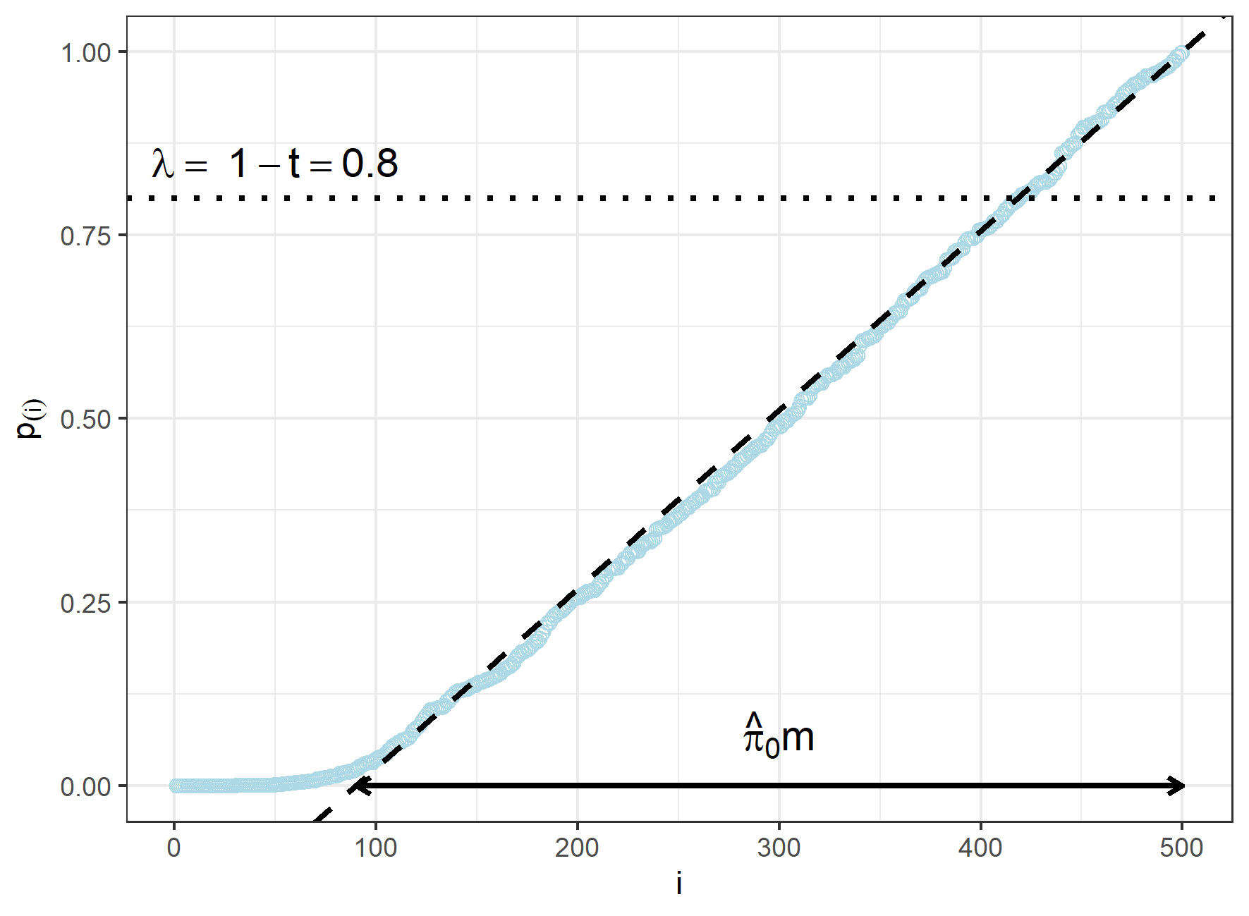
Figure 1: Illustration of the computation of the Schweder-Spjøtvoll-Storey estimate $\hat{\pi}_{0}$, based on 500 sorted simulated p-values. The dashed, straight line is constructed in such a way that it goes through both (500,1) and the point where the dotted line intersects the curve of p-values, roughly speaking.

2.3 Median unbiased estimation of the FDP

Define the FDP to be the proportion of false positives,

$$FDP=\frac{V}{R},\quad FDP(t)=\frac{V(t)}{R(t)},$$

which is understood to be $0$ when $R=0$. The median unbiased estimate $\overline{V}$ immediately implies a median unbiased estimate of the FDP.

Theorem 2.

Suppose Assumption 1 is satisfied. The variable $\overline{FDP}(t)=\overline{V}(t)/R(t)$ is a median unbiased estimator for the FDP, i.e.,

$$\mathbb{P}(FDP(t)\leq\overline{FDP}(t))\geq 0.5.$$ (8)

To prove this, we only need to remark that if $V\leq\overline{V}$, then $FDP\leq\overline{FDP}$.

A more positive perspective is that we obtain a $50\%$-confidence lower bound $\underline{S}=R-\overline{V}$ for the number of true discoveries, $S=R-V$. This estimator satisfies $\mathbb{P}(\underline{S}\leq S)\geq 0.5$. Further, the true discovery proportion (Andreella et al., 2020; Goeman et al., 2021; Vesely et al., 2021; Blain et al., 2022) is

$$TDP=\frac{S}{R}=\frac{m-V}{R}.$$

A $50\%$-confidence lower bound for the TDP is

$$\underline{TDP}=\frac{\underline{S}}{R}=\frac{m-\overline{V}}{R},$$

i.e., we have $\mathbb{P}(\underline{TDP}\leq TDP)\geq 0.5.$

3 Controlling the mFDP

3.1 Overview of our method and comparison with FDR control

In section 2.3 we considered a fixed rejection threshold $t$ and provided a median unbiased estimate for $FDP(t)$. In many situations, one would like to adapt the threshold $t$ based on the data, in such a way that one still obtains a valid median unbiased estimate. Note that naively choosing $t$ in such a way that an attractive (low) estimate of the FDP is obtained, can invalidate the procedure, in the sense that inequality (8) not longer holds. In the present section however, we derive a method that provides median unbiased bounds for a large range of $t$, in such a way that with probability at least $0.5$, the bounds are simultanously valid for all $t$.

Specifically, we let the user choose some range $\mathbb{T}\subseteq[0,1]$ of rejection thresholds $t$ of interest, before looking at the data. Usually a good choice for $\mathbb{T}$ will be $[0,1/2]$ or another interval starting at $0$. Then we provide $50\%$-confidence upper bounds $B(t)$ for $V(t)$ that are simultaneously valid over all $t\in\mathbb{T}$:

$$\mathbb{P}\Big{(}\bigcap_{t\in\mathbb{T}}\{V(t)\leq B(t)\}\Big{)}\geq 0.5.$$ (9)

It then immediately follows that $B(t)/R(t)$, $t\in\mathbb{T}$, are simultaneously valid $50\%$-confidence bounds for $FDP(t)$:

$$\mathbb{P}\Big{(}\bigcap_{t\in\mathbb{T}}\{FDP(t)\leq B(t)/R(t)\}\Big{)}\geq 0.5.$$

Since the threshold $t$ can be chosen based on the data, it can be picked such that $B(t)/R(t)$ is low. In particular, one can prespecify a value $\gamma\in[0,1]$, for example $\gamma=0.05$, and take the threshold $t\in\mathbb{T}$ to be the largest value for which $B(t)/R(t)\leq\gamma$, if such a $t$ exists. This means that our method can be used to reject a set of hypotheses in such a way that the median of the FDP is bounded by $\gamma$:

$$\mathbb{P}(FDP\leq\gamma)\geq 0.5.$$

In other words, we can control the median of the FDP, which we will call the mFDP. Our notation ‘$\gamma$’ is in line with e.g. Romano and Wolf (2007) and Basu et al. (2021).

Our method is related to the popular BH procedure, which ensures that $\mathbb{E}(FDP)\leq\gamma$ (Benjamini and Hochberg, 1995). BH ensures that the mean of the FDP is controlled, while we ensure that the median of the FDP is controlled. The mean and the median of the FDP can be asymptotically equal in some settings where the dependencies among the p-values are not too strong (Neuvial, 2008; Ditzhaus and Janssen, 2019), but there is no general guarantee that they are similar (Romano and Shaikh, 2006; Schwartzman and Lin, 2011). Especially under strong dependence, $mFDP\leq\gamma$ does not need to imply $\mathbb{E}(FDP)\leq\gamma$, while the converse does hold in many practical situations. Moreover, unlike mFDP control, FDR control always implies weak control of the family-wise error rate (Romano et al., 2008, Section 6.4). Note, however, that before applying any multiple testing method, we could first perform a global test, to enforce weak family-wise error rate control (Bernhard et al., 2004). Moreover, our method combines good power with simultaneity, as we will now discuss.

The most important advantage of our method over BH, is that it provides simultanous 50% confidence bounds for the FDP. This allows simultaneous as well as post hoc inference, in the sense that $t\in\mathbb{T}$ can be chosen after seeing the data. In particular our method adapts to the amount of signal in the data: if there is much signal, we can find very low upper bounds for the FDP and if there is little signal, we tend to find higher bounds for the FDP.

The simultaneity of our bounds also has implications for mFDP control. Note that Benjamini-Hochberg requires fixing the FDR bound beforehand. The FDR bound is often called $\alpha$ and is analogous to our $\gamma$. There is then a risk to reject nothing at all, even if there is quite some signal in the data. BH does then not allow increasing $\gamma$, since $\gamma$ is required to be data-independent. Our method, however, allows the user to change $\gamma$ and still obtain valid results. mFDP control and mFDP-adjusted p-values are treated in Sections 3.4 and 3.5.

3.2 Simultaneous bounds for the FDP

Let $\mathbb{N}$ be the set of natural numbers. We call a function $B:\mathbb{T}\rightarrow\mathbb{N}$ a confidence envelope is it satisfies inequality (9) (cf. Hemerik et al., 2019). We restrict ourselves to such 50% confidence envelopes and do not consider e.g. 95% confidence envelopes. Let $\mathbb{B}$ be a set of maps $\mathbb{T}\rightarrow\mathbb{N}$. Assume that $\mathbb{B}$ is monotone, in the sense for all $B,B^{\prime}\in\mathbb{B}$, either $B\geq B^{\prime}$ or $B^{\prime}\geq B$. Here $B\geq B^{\prime}$ means that $B(t)\geq B^{\prime}(t)$ for all $t\in\mathbb{T}$. We call $\mathbb{B}$ the family of candidate envelopes (cf. Hemerik et al., 2019).

We will obtain a confidence envelope by picking the smallest $B\in\mathbb{B}$ for which $B(t)\geq\overline{V}^{\prime}(t)$ for all $t\in\mathbb{T}$. We call this envelope $\tilde{B}$:

$$\tilde{B}=\tilde{B}(p)=\min\Big{\{}B\in\mathbb{B}:\bigcap_{t\in\mathbb{T}}\big{\{}B(t)\geq\overline{V}^{\prime}(t)\big{\}}\Big{\}},$$

If $r$ is a vector containing, say, $l_{r}$ p-values, then we write $\mathcal{R}(r,t)=\{1\leq i\leq l_{r}:r_{i}<t\}$, to make the dependence on the p-values explicit. Analogously we define ${V}(r,t)$, $\overline{V}^{\prime}(r,t)$ and $\tilde{B}(r)$. We use the convention that $\mathcal{R}(t)=\mathcal{R}(p,t)$, ${V}(t)={V}(p,t)$, $\overline{V}^{\prime}(t)=\overline{V}^{\prime}(p,t)$ and $\tilde{B}=\tilde{B}(p)$.

We will only require Assumption 2 below. Due to the monotonicity of the set $\mathbb{B}$, we always have either $\tilde{B}(q)\geq\tilde{B}(1-q)$ or $\tilde{B}(q)<\tilde{B}(1-q)$. The assumption is satisfied in particular if the probability that the latter inequality holds is not larger than the probability of the former. The assumption is a generalization of Assumption 1, in the sense that if $\mathbb{T}$ is equal to the singleton $\{t\}$ then Assumptions 1 and 2 will coincide, for most reasonable choices of $\mathbb{B}$.

Assumption 2.

The following holds:

$$\mathbb{P}\big{\{}\tilde{B}(p)\geq\tilde{B}(1-q)\big{\}}\geq 0.5,$$ (10)

Note that Assumption 2 is satisfied in particular if $\mathbb{P}\big{\{}\tilde{B}(q)\geq\tilde{B}(1-q)\big{\}}\geq 0.5$. Assumption 2 always holds if property (5) is satisfied, hence in particular under independence. However, property (5) is not necessary for Assumption 2 to hold, as confirmed by all our simulations.

Let $[\cdot]^{+}$ be the positive part function. The following theorem states that $\tilde{B}$ provides simultaneously valid $50\%$-confidence bounds.

Theorem 3.

Suppose Assumption 2 holds. Then the function $\tilde{B}$ is a confidence envelope, i.e.,

$$\mathbb{P}\Big{(}\bigcap_{t\in\mathbb{T}}\{V(t)\leq\tilde{B}(t)\}\Big{)}\geq 0.5$$

and

$$\mathbb{P}\Big{(}\bigcap_{t\in\mathbb{T}}\{FDP(t)\leq\tilde{B}(t)/R(t)\}\Big{)}\geq 0.5.$$

In addition, $\tilde{B}^{\prime}:\mathbb{T}\rightarrow\mathbb{N}$ defined by

$$\tilde{B}^{\prime}(t)=R(t)-\max\{[R(l)-\tilde{B}(l)]^{+}:l\in\mathbb{T},l\leq t)\},$$

which satisfies $\tilde{B}^{\prime}\leq\tilde{B}$, is also a confidence envelope and potentially improves $\tilde{B}$.

In the rest of this subsection, we provide an extention of the bounds $\tilde{B}^{\prime}(t)$ and a result on admissibility. It turns out that $\tilde{B}^{\prime}$ coincides with an envelope obtained through a novel closed testing-based procedure, in the sense of Goeman and Solari (2011) and Goeman et al. (2021). This novel procedure provides a $50\%$ confidence bound for the number of true hypotheses in $I$, for every subset $I\subseteq\{1,...,m\}$. These bounds are all simultaneously valid with probability at least $50\%$. We denote these bounds by $\overline{B}(I)$.

Theorem 4.

Write $\mathcal{M}=\{I\subseteq\{1,...,m\}:I\neq\emptyset\}.$ For every $I\in\mathcal{M}$ and $t\in\mathbb{T}$, define $R_{I}(t):=|\mathcal{R}(t)\cap I|=|\{i\in I:p_{i}\leq t\}|$. Write

$$\overline{B}(I):=\max\{|A|:\emptyset\neq A\subseteq I\text{ and }\forall t\in\mathbb{T}:R_{A}(t)\leq\tilde{B}^{\prime}(t)\}.$$ (11)

where the maximum of an empty set is interpreted as 0.

Assume $\mathbb{T}\subseteq[0,1/2)$ and $\mathbb{P}\big{\{}\tilde{B}(q)\geq\tilde{B}(1-q)\big{\}}\geq 0.5$. Then

$$\mathbb{P}\Big{[}\bigcap_{I\in\mathcal{M}}\big{\{}|\mathcal{N}\cap I|\leq\overline{B}(I)\big{\}}\Big{]}\geq 0.5,$$

i.e., the $\overline{B}(I)$ are simultaneous $50\%$ confidence bounds for the number of true hypotheses in $I$. In particular, the function $\mathbb{T}\rightarrow\mathbb{N}$ defined by $t\mapsto\overline{B}(\mathcal{R}(t))$ is a confidence envelope.

It follows from Theorem 3 in Goeman et al. (2021) that if the local tests discussed in the proof of Theorem 4 are admissible, then the procedure of Theorem 4 is admissible. The latter means that there exists no procedure that is uniformly more powerful. By Theorem 5 below it then follows that the envelope $\tilde{B}^{\prime}(t)$ from Theorem 3 is also admissible. The local tests will usually be admissible when $\mathbb{B}$ is any reasonable family, for example the family considered in Section 3.3.

Theorem 5.

For every $t\in\mathbb{T}$, the bound $\tilde{B}^{\prime}(t)$ from Theorem 3 is equal to the bound $\overline{B}(\mathcal{R}(t))$ from Theorem 4. Moreover, if the procedure from Theorem 4 that provides bounds for all $I\in\mathcal{M}$ is admissible, then the envelope $\tilde{B}^{\prime}$ is also admissible. Here admissibility of $\tilde{B}^{\prime}$ means that there exists no envelope $B:\mathbb{T}\rightarrow\mathbb{N}$ such that $B(t)\leq\tilde{B}^{\prime}(t)$ for all $t\in\mathbb{T}$ and such that $\mathbb{P}\{\exists t\in\mathbb{T}:B(t)<\tilde{B}^{\prime}(t)\}>0.$

In the rest of this paper we will only focus on bounds for rejected sets of the form $\mathcal{R}(t)=\{1\leq i\leq m:\text{ }p_{i}\leq t\}$, as constructed in Theorem 3.

3.3 A default mFDP envelope

The envelope $\tilde{B}$ depends on a general family $\mathbb{B}$ of candidate confidence bounds. The choice of this family can have a large influence on the bounds obtained (cf. Hemerik et al., 2019). An important question is thus how to choose this set $\mathbb{B}$ in a suitable way. Typically we want $\mathbb{B}$ to contain at least one function $B$ that is a tight upper envelope of the function $t\mapsto\overline{V}(t)$. Note that between $t=0$ and, say, $t=0.5$, the function $\overline{V}^{\prime}(t)$ tends to be roughly linear in $t$, at least under under indepedence. Thus, it can make sense to also take the candidate envelopes $B\in\mathbb{B}$ to be roughly linear. Also, giving them a small positive intercept will often be useful to avoid that $\tilde{B}$ is too sensitive to p-values near 1.

Further, it is usually suitable to take $\mathbb{T}=[s_{1},s_{2}]$, where $s_{1}\geq 0$ is the smallest threshold of interest and $s_{2}<1$ is the largest threshold of interest. Based on these considerations, we propose to use the following default family $\mathbb{B}$ of candidate functions:

$$\mathbb{B}=\{B^{\kappa}:\kappa\in(0,\infty]\},$$ (12)

with

$$B^{\kappa}(t)=|\{1\leq i\leq m:i\kappa-c\leq t\}|=\Big{\lfloor}\frac{t+c}{\kappa}\Big{\rfloor}.$$

Here, $c\geq 0$ is a pre-specified small constant. The discrete function $B^{\kappa}$ is roughly linear in $t$ and has slope $1/\kappa$.

The choice of $c$ influences the slope and intercept of $B^{\kappa}$ and hence of the resulting envelope $\tilde{B}$. Taking $c$ to be $0$ or very small tends to lead to tighther bounds $\tilde{B}(t)$ for very small $t$, while taking $c$ a bit larger tends to lead to tighter bounds for larger $t$. We found in simulations that taking $c=1/(2m)$ usually gave good overall power.

If we take $\mathbb{B}$ as in expression (12), then the confidence envelope becomes

$$\tilde{B}=B^{\kappa_{\text{max}}}\text{, where }\quad\kappa_{\text{max}}=\max\Big{\{}\kappa\in(0,\infty]:\bigcap_{t\in\mathbb{T}}\big{\{}B^{\kappa}(t)\geq\overline{V}^{\prime}(t)\big{\}}\Big{\}}.$$ (13)

For computer programming this method, a useful equivalent formulation is the following, if $\mathbb{T}$ is an interval.

Proposition 2.

Suppose $\mathbb{T}$ is of the form $[s_{1},s_{2}]$, with $0\leq s_{1}<s_{2}\leq 1$. We then have

$$\kappa_{\text{max}}=\kappa_{0}\wedge\min\Big{\{}\kappa_{i}:1\leq i\leq m\text{ and }1-p_{i}\in\mathbb{T}\Big{\}},$$ (14)

where

$$\kappa_{0}=\frac{s_{1}+c}{\overline{V}^{\prime}(s_{1})}=\frac{s_{1}+c}{|\{1\leq j\leq m:\text{ }p_{j}\geq 1-s_{1}\}|}$$

and for $1\leq i\leq m$

$$\kappa_{i}=\frac{1-p_{i}+c}{\overline{V}^{\prime}(1-p_{i})}=\frac{1-p_{i}+c}{|\{1\leq j\leq m:\text{ }p_{j}\geq p_{i}\}|}.$$

(If the denominator is 0, the expression is interpreted as $\infty$.)

Note that we can sometimes straightforwardly improve the envelope $B^{\kappa_{\text{max}}}$ by using the second part of Theorem 3. In Example 2, we continue the running example and compute simultaneous mFDP bounds. Figure 2 shows the confidence envelope and Figure 3 illustrates how the envelope was determined.

Example 2 (Running example, part 2: Confidence envelopes.).

We continue on Example 1 by computing confidence envelopes, i.e., simultaneous $50\%$-confidence upper bounds for $V(t)$, the number of false positives, which depends on the threshold $t$. We took $\mathbb{T}=[0,0.2]$ and defined $\tilde{B}$ as in (13). We computed $\tilde{B}$ for both $c=0$ and $c=2/m=0.004$. These choices for $c$ were somewhat arbitrary. The number of rejections $R(t)$, as well as the bounds $\tilde{B}(t)$ for both values of $c$, are plotted in Figure 2. The construction of the confidence envelopes $\tilde{B}$ is illustrated in Figure 3.

The figure shows that as expected, near $t=0$, the number of rejections increases quickly with $t$. The reason is that there were many p-values near 0, as seen in Figure 1. By definition (13), the bounds $\tilde{B}(t)$ are roughly linear in $t$ and we see this in the figures. We also see that for this specific dataset, the bound $\tilde{B}$ depends strongly on $c$: for $c=0.004$, the bound $\tilde{B}(t)$ is lower than for $c=0$ if $t$ is close to $0$, but much higher otherwise. For most values of $t\in[0,1]$ the envelope for $c=0.004$ is better, i.e. lower, than the envelope for $c=0$. On the other hand, the smallest cutoffs are often most relevant. Finally, we remark that the bounds in the figures can be somewhat improved using the last part of Theorem 3. This improvement was used to obtain Figure 4, where simultaneous $50\%$ confidence bounds for $FDP(t)$ are shown.

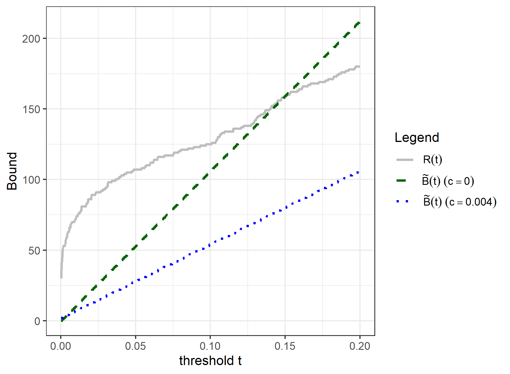
Figure 2: Graph showing the number of of rejections and two confidence envelopes for the running example. The solid line shows the number of rejections, which depends on the rejection threshold $t$. The other lines are two confidence envelopes $\tilde{B}$. These are simultaneous $50\%$-confidence upper bounds for the number of false positives $V(t)$. The intercept and slope of $\tilde{B}$ depend on the user-specified constant $c$. Note that for $c=0$, the intercept is slightly smaller than for $c=0.004$. Indeed, the intercepts are 0 and 2 respectively.

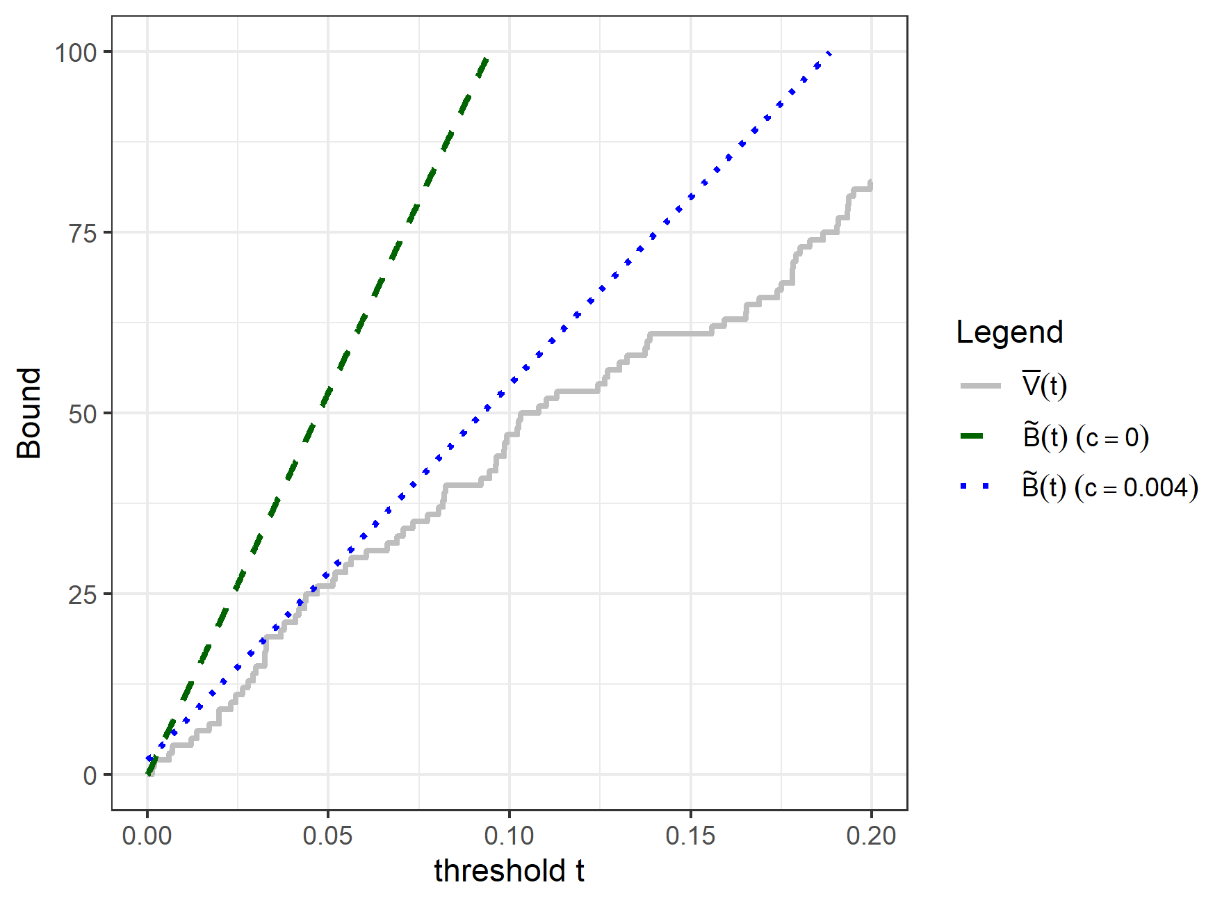
Figure 3: Illustration of the construction of the confidence envelope for the running example. For every rejection threshold $t$, $\overline{V}(t)$ is a $50\%$ confidence upper bound for the number of false positives, $V(t)$. The confidence envelope $\tilde{B}(t)$ is constructed in such a way that it lies above the pointwise bound $\overline{V}(t)$ for all $t\in\mathbb{T}$. Due to this construction, the bounds $\tilde{B}(t)$ are simultaneous $50\%$-confidence bounds for $V(t)$. The intercept and slope of $\tilde{B}$ are influenced by the choice of $c$.

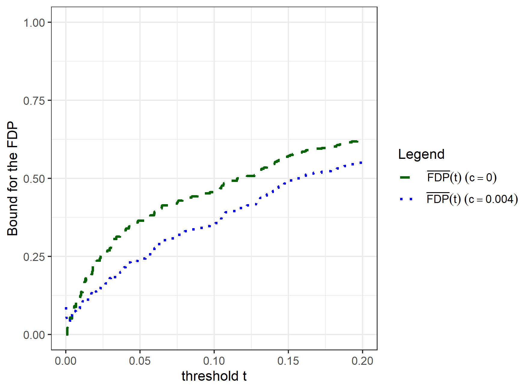
Figure 4: For two values of $c$, simultaneous $50\%$ confidence upper bounds for $FDP(t)$ are shown. Here $\overline{FDP}(t):=\tilde{B}(t)/R(t)$. Note that if $c=0.004$, the bound is larger than zero at $t=0$. The reason is that $\tilde{B}(0)>0$ for this value of $c$. Roughly speaking, the bound $\overline{FDP}(t)$ then decreases for a while, before it starts to increase. Note that if $c=0$, then the bound starts at zero and increases from there.

3.4 Controlling the median of the FDP

Consider $\gamma\in[0,1]$. As discussed in section 3.1, we can use any confidence envelope $B$ to guarantee that $\mathbb{P}(FDP\leq\gamma)\geq 0.5.$ In other words, we can control the mFDP. Note that by $mFDP$ we mean the median of the distribution that the FDP has, conditional on the data and conditional on $\gamma$, which can be chosen after seeing the data. This is stated in the following Theorem. (The maximum of an empty set is taken to be 0.)

Theorem 6.

Let $B:\mathbb{T}\rightarrow\mathbb{N}$ be a confidence envelope, for example $\tilde{B}$. Let the target FDP $\gamma\in[0,1]$ be freely chosen based on the data. Define

$$t_{\text{max}}=t_{\text{max}}(B,\gamma)=\max\{p_{i}:\text{ there is a }t\in\mathbb{T}\cap[p_{i},1]:B(t)/R(t)\leq\gamma\}.$$

Reject all hypotheses with p-values at most $t_{\text{max}}$ and denote the FDP by $FDP_{\gamma}$. Then with probability 0.5 the FDP is at most $\gamma$, i.e.,

$$\mathbb{P}\big{\{}FDP_{\gamma}\leq\gamma)\big{\}}\geq 0.5.$$ (15)

In fact we have

$$\mathbb{P}(\bigcap_{\gamma\in[0,1]}FDP_{\gamma}\leq\gamma)\geq 0.5,$$ (16)

i.e., the procedure offers mFDP control simultaneously over all $\gamma\in[0,1]$.

In other words, if we reject all hypotheses with p-values that are at most $t_{\text{max}}$, then a median unbiased estimate of the FDP is $\gamma$. This follows directly from the fact that the estimates $\overline{FDP}(t)$, $t\in\mathbb{T}$, are simultaneously valid $50\%$-confidence upper bounds, by inequality (9). Inequality (15) holds despite the fact that $\gamma$ can depend on the data. In fact, with probability at least $50\%$, $FDP_{\gamma}\leq\gamma$ simultaneosly over all $\gamma\in[0,1]$. This contrasts our method with many other procedures, which require considering only one rejection criterion, which moreover needs to be chosen in advance (Benjamini and Hochberg, 1995; van der Laan et al., 2004; Lehmann and Romano, 2005; Romano and Wolf, 2007; Guo and Romano, 2007; Roquain, 2011; Neuvial, 2008; Guo et al., 2014; Delattre and Roquain, 2015; Ditzhaus and Janssen, 2019; Döhler and Roquain, 2020; Basu et al., 2021; Miecznikowski and Wang, 2022). In Example 3 we continue the running example and apply our mFDP control method.

Example 3 (Running example, part 3: Controlling the mFDP.).

We continue on Example 2. Take $\gamma=0.05$ and consider the confidence envelope $\tilde{B}$ discussed in Example 2. To find a rejection threshold $t_{\text{max}}$ for which we can ensure $mFDP\leq\gamma$, we use Theorem 6. It computes $t_{\text{max}}$ as the largest $t$ for which the estimate in Figure 4 is at most $\gamma$.

Recall that in Example 3, we computed bounds $\tilde{B}(t)$ for both $c=0$ and $c=0.004$. For $c=0$, we now find $t_{\text{max}}=0.002709$, which is the 54-th smallest p-value. Thus, we can reject 54 hypotheses. More precisely, if we reject the 54 smallest p-values, we know that the mFDP is below $\gamma=0.05$. Note that $t_{\text{max}}$ is about 27 times higher than the Bonferroni threshold $0.05/500=0.0001$.

If $c=0.004$ then $t_{\text{max}}=0.001660$, so that we can only reject 53 hypotheses. The reason why $t_{\text{max}}$ is lower if $c=0.004$, it that for small values of $t$, the bound $\tilde{B}(t)$ is higher for $c=0.004$ than for $c=0$. We saw this in Figure 2.

Note that it is allowed to change $\gamma$ after looking at the data. For instance, if we decrease $\gamma$ to 0.01, we reject 44 hypotheses if $c=0$ and we reject no hypotheses for $c=0.004$.

3.5 Adjusted p-values for mFDP control

Adjusted p-values can be a useful tool in multiple testing. They are defined as the smallest level, e.g. the smallest $\gamma$, at which the multiple testing procedure would reject the hypothesis. Adjusted p-values can be problematic in the context of e.g. FDR control and ours. The reason is that the adjusted p-value does not have an independent meaning and can easily be misinterpreted when taken out of context (Goeman and Solari, 2014, §5.4). Moreover, an mFDP-adjusted p-value could be $0$, which also shows that the interpretation is very different than for real p-values, which cannot be $0$. Nevertheless, in our context, adjusted p-values are quite useful, because, once computed, they allow checking quickly which hypotheses are rejected for various $\gamma$.

Let $B$ be a confidence envelope and $1\leq i\leq m$. As discussed in Section 3.4, $B$ defines an mFDP controlling procedure. The mFDP adjusted p-value for $H_{i}$ is the largest $\gamma\in[0,1]$ for which $H_{i}$ is still rejected by the mFDP controlling procedure. Consequently, if we reject all hypotheses $H_{i}$ with $p_{i}^{\text{ad}}\leq\gamma$, then $mFDP\leq\gamma$.

Proposition 3.

Let $1\leq i\leq m$. Then the value

$$p_{i}^{\text{ad}}:=\min\{B(t)/R(t):t\in\mathbb{T}\cap{[p_{i},1]}\},$$ (17)

is an mFDP-adjusted p-value for $H_{i}$, i.e., if we reject all hypotheses $H_{i}$ with $p_{i}^{\text{ad}}\leq\gamma$, then $\mathbb{P}(FDP_{\gamma}\leq\gamma)\geq 0.5$. Here $\gamma$ may be chosen based on the data. In fact, inequality (16) holds. We take the minimum of an empty set to be $\infty$.

Suppose $\mathbb{T}$, the set of rejection thresholds of interest, is of the form $[s_{1},s_{2}]$. Then we have the following useful reformulation of Proposition 3.

Proposition 4.

Suppose $\mathbb{T}$ is of the form $[s_{1},s_{2}]$, with $0\leq s_{1}<s_{2}\leq 1$. For each $1\leq i\leq m$ with $p_{i}\leq s_{2}$, the adjusted p-value defined above is then

$$p_{i}^{\text{ad}}=\min\Big{\{}B(t)/R(t):t\in\big{[}\max\{s_{1},p_{i}\},s_{2}\big{]}\cap\big{\{}s_{1},p_{1},p_{2},...,p_{m}\big{\}}\Big{\}}.$$ (18)

Note that given the data, the adjusted p-value is non-decreasing function of the unadjusted p-value. As a consequence of this and Proposition 4, if $\mathbb{T}$ is of the form $[s_{1},s_{2}]$, we can use Algorithm 1 to efficiently compute the mFDP adjusted p-values. The algorithm takes the $m$ sorted p-values, $p_{(1)},...,p_{(m)}$, as input and returns the corresponding sorted adjusted p-values.

The idea of the algorithm is to start with computing the largest adjusted p-value(s), continue with the second largest one and so on. The algorithm also uses the fact that if $p_{(i)}>s_{2}$, then $p_{(i)}^{\text{ad}}=\infty$. It further uses the fact that all hypotheses with unadjusted p-values below $s_{1}$ have the same adjusted p-value. Adjusted p-values can be easily computed using the R package mFDP.

Algorithm 1 Algorithm for computing the mFDP adjusted p-values if $\mathbb{T}=[s_{1},s_{2}]$

  $r\leftarrow|\{1\leq i\leq m:\text{ }p_{i}\leq s_{2}\}|$.

  if $r<m$ then

     $p_{(r+1)}^{\text{ad}},...,p_{(m)}^{\text{ad}}\leftarrow\infty$.

  end if

  if $r>0$ then

     if $s_{1}\leq p_{(r)}$ then

        $p_{(r)}^{\text{ad}}\leftarrow B(p_{(r)})/R(p_{(r)})$

     else

        $p_{(r)}^{\text{ad}}\leftarrow B(s_{1})/R(s_{1})$

     end if

     $l\leftarrow r-1$

     $continue\leftarrow FALSE$

     if $l>0$ then

        if $s_{1}\leq p_{(l)}$ then

           $continue\leftarrow TRUE$

        end if

     end if

     while $continue=TRUE$ do

        $p_{(l)}^{\text{ad}}=\min\{p_{(l+1)}^{\text{ad}},B(p_{(l)})/R(p_{(l)})\}$

        $l\leftarrow l-1$

        if $l=0$ then

           $continue\leftarrow FALSE$

        else

           if $p_{(l)}<s_{1}$ then

              $continue\leftarrow FALSE$

           end if

        end if

     end while

     if $0<l$ then

        $p_{(1)}^{\text{ad}},...,p_{(l)}^{\text{ad}}\leftarrow\min\{p_{(l+1)}^{\text{ad}},B(s_{1})/R(s_{1})\}$

     end if

  end if

  return  $p_{(1)}^{\text{ad}},...,p_{(m)}^{\text{ad}}$

4 Simulations

We performed simulations to assess the error control and power of our method. We also compared our method to BH (Benjamini and Hochberg, 1995; Benjamini and Yekutieli, 2001), which is the most popular method related to FDP control.

In the simulations we considered $m=1000$ hypotheses. The p-values were based on Z statistics, computed from simulated data with various dependence structures. The p-values were two-sided, unless stated otherwise. To add signal a number $\Delta$ was added to the first $(1-\pi_{0})/m$ test statistics. The following dependence structures of the test statistics were considered:

• independence (IN);

• homogeneous positive correlations $\rho$ (HO);

• five independent blocks, with positive dependence $\rho$ within blocks (BL);

• 50 negatively dependent blocks (correlations -0.01), with correlation 0.5 within blocks. The p-values were right-sided, so that they were negatively correlated between blocks (NE).

Further, we varied $\pi_{0}$, the signal $\Delta$ and correlation strength $\rho$.

We computed $\tilde{B}$ as in Section 3.3. We took $\mathbb{T}=[0,0.1]$, i.e. our bounds and mFDP-adjusted p-values were simultaneously valid with respect to all thresholds $t$ in this interval. We took $c=1/(2m)=0.0005$, as recommended in Section 3.3 .

We first assessed whether our method provided appropriate simultaneous mFDP control. We show simulation results in Table 1. For each setting, the table shows the estimate of the probability $\mathbb{P}\{\text{for some }t\in\mathbb{T}\text{, }V(t)>\tilde{B}(t)\}$, which is identical to the probability that there is a $0<\gamma<1$ for which $FDP_{\gamma}$ exceeds $\gamma$. Each estimate was based on $10^{4}$ repeated simulations. The simulations in this section took less than one hour in total on a standard PC.

The table confirms the simultaneous control of our method. We see that the estimated error rate is about $0.5$ under independence if $\pi_{0}=1$. Indeed, the true error rate is then exactly 0.5. The reason is that then $p=q$ and the equality (5) then holds, so that the probability in expression (2) is exactly $0.5$. We see that for $\pi_{0}=0.95$, the error rate is also about $0.5$, rather than less. This is because our method is rather adaptive, as mentioned in the Introduction. In the setting with negative dependence and $\pi_{0}=1$ and one-sided p-values, the error rate is also exactly 0.5, again because (5) then holds. Note that in the other cases, the method was also valid.

Table 1: For various settings, the last column indicates the simulation-based estimate of the probability that there is a $0<\gamma<1$ for which $FDP_{\gamma}$ exceeds $\gamma$. This probability should not be larger than $0.5$. For the settings with $\pi_{0}<1$, the signal for the false hypotheses was $\Delta=3$.

$\pi_{0}$	Setting	$\rho$	$\mathbb{P}(\text{error})$
1	IN	$0$	.499
1	HO	$.2$	.334
1	HO	$.5$	.266
1	HO	$.9$	.330
1	BL	$.5$	.335
1	BL	$.9$	.351
1	NE	$-.01$	.500
.95	IN	$0$	.498
.95	HO	$.2$	.336
.95	HO	$.5$	.266
.95	HO	$.9$	.327
.95	BL	$.5$	.338
.95	BL	$.9$	.343
.95	NE	$-.01$	.501

Next, we assessed the power of our method and compared to the power of BH. The power was defined as the average fraction of false hypotheses that were rejected. In each simulation loop, we calculated mFDP- and FDR-adjusted p-values and recorded which p-values were below $\gamma$, for three values of $\gamma$. For BH1995, we took $\alpha=0.05$. BH does not have a simultaneity property, so we only show simulation results for this value of $\alpha$ for BH. We took $\pi_{0}=0.9$, i.e., the first 100 hypotheses were false. The results are shown in Table 2.

Table 2: For various simulation settings, the power of our method is shown as depending on $\gamma$. The last column shows the power of BH, for $\alpha=0.05$. Since our method provides simultaneous inference, $\gamma$ may freely be chosen after seeing the data and we have mFDP control simultaneously over all $\gamma\in[0,1]$. Since BH requires choosing $\alpha$ beforehand, we only show its power for one value of $\alpha$.

			$\gamma$ (i.e., $\alpha$)
Setting	$\rho$	$\Delta$	0.01	0.05	0.1	0.05(BH)
IN	0	$2$	.043	.045	.084	.059
IN	0	$3$	.224	.431	.557	.495
IN	0	$4$	.538	.848	.901	.878
HO	.5	$2$	.066	.102	.139	.099
HO	.5	$3$	.216	.393	.505	.466
HO	.5	$4$	.513	.854	.916	.860
BL	.8	$2$	.057	.123	.175	.127
BL	.8	$3$	.235	.436	.533	.476
BL	.8	$4$	.553	.818	.877	.839
NE	-.01	$2$	.068	.100	.171	.120
NE	-.01	$3$	.281	.539	.666	.600
NE	-.01	$4$	.593	.895	.940	.919

Table 2 shows that for $\gamma=0.05$, the power of our method was roughly equal to that of BH, yet often slightly lower. However, our method provides simultaneous inference, meaning that our bounds are simultaneous and $\gamma$ can be chosen after seeing the results.

As expected, the power of our method increased with $\gamma$. Note that for in the independence setting “IN”, for $\Delta=2$, there was only a small difference between the power for $\gamma=0.01$ and $\gamma=0.05$. This is because the number of rejections was nearly always low in this setting and the envelope $\tilde{B}$ is discrete, so that $\overline{FDP}(t)$ usually made large jumps as a function of $t$.

5 Data analysis

We analyzed part of the RNA-Seq count data discussed in Best et al. (2015). The data are from 283 blood platelet samples. We downloaded the data from the Gene Expression Omnibus, accession GSE68086. The samples are from patients with one of six types of cancer, as well as controls. We used the data from the 35 patients with pancreatic cancer and the 42 patients with colorectal cancer (n=77). The data contain read counts of 57736 transcripts. We removed the data on transcripts for which more than $75\%$ of the counts were 0, resulting in data on 10042 transcripts.

For each of the $m=10042$ transcripts, we tested the null hypothesis of no association with type of cancer, i.e, pancreatic or colorectal. To compute the $m$ raw p-values, we used the R package DE-Seq2, which is currently the most standard approach (Love et al., 2014). This method employs a negative binomial model for each transcript.

We used the computed raw p-values as input for our method of Sections 3.3-3.5. The method requires choosing the tuning parameter $c$ a priori. We chose $c=1/(2m)$, as recommended in Section 3.3 and used in the simulations. Figure 5 shows the number of rejections and the simultaneous bound for the number of false positives, as functions of the rejection threshold $t$. Note that for small thresholds, $R(t)$ is much larger than $\tilde{B}(t)$, so that the $mFDP$ is small. Note that roughly speaking, $R(t)$ increased faster in $t$ than $\tilde{B}(t)$. Consequently, the improved envelope $\tilde{B}^{\prime}(t)$ from the second part of Theorem 3 was almost identical to $\tilde{B}(t)$. In Figure 6 the corresponding simultaneous $50\%$-confidence upper bounds for the FDP are shown.

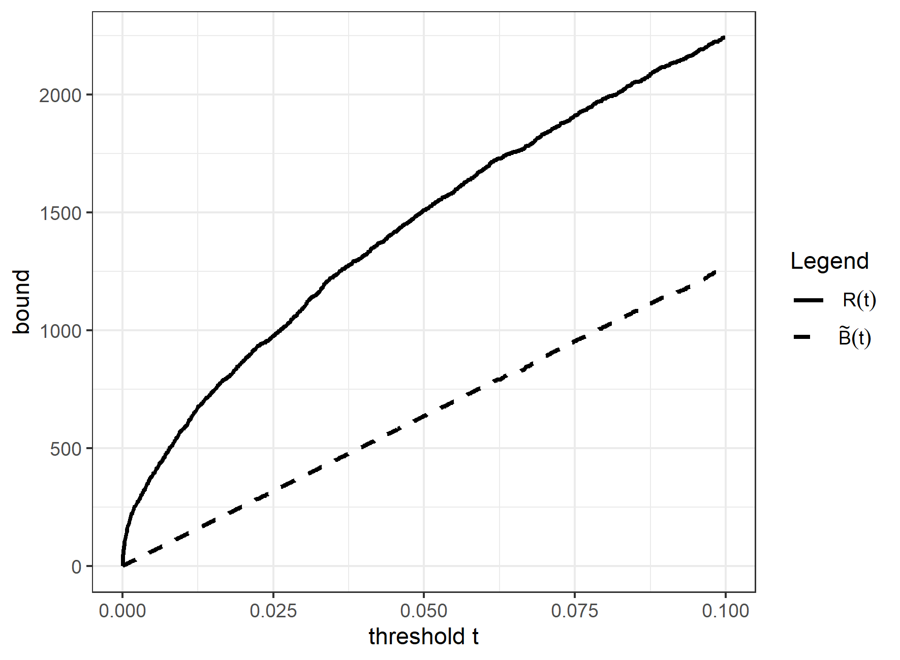
Figure 5: The number of rejections and the simultaneous bound for the number of false positives, as functions of the rejection threshold $t$.

Figure 6: The simultaneous $50\%$-confidence upper bound $\overline{FDP}(t):=\tilde{B}^{\prime}(t)/R(t)$ as function of the rejection threshold $t$. For several values of $t$, $R(t)$ is shown at the top of the graph.

We used Algorithm 1 to compute mFDP-adjusted p-values. These are useful, because the number of hypotheses that the method rejects can be computed as the number of adjusted p-values that are at most $\gamma$. We used the adjusted p-values for generating Table 3, where the number of rejections is shown for various values of the mFDP-threshold $\gamma$. For comparison, we also show the number of rejections with BH for $\alpha=\gamma$. Note, however, that BH only allows using one value for $\alpha$, which moreover needs to chosen before seeing the data.

Table 3: For different values of $\gamma$, the number of rejected null hypotheses is shown, for two methods. The first method is our method for simultaneous mFDP control. The inferences with this method are simultaneous, which means that with $50\%$ confidence, $FDP_{\gamma}\leq\gamma$ for all $\gamma\in\mathbb{T}$ simultaneously. The second method is BH, which ensures that if $\alpha$ is chosen prior to the data analysis, then $FDR=FDR(\alpha)\leq\alpha$, but not simultaneously over multiple $\alpha$.

	$\gamma$ (i.e., $\alpha$)
Method	0.01	0.05	0.1
mFDP control	24	125	243
FDR control with BH	12	163	287

The interpretation of the table is as follows. If the user first chooses e.g. $\gamma=0.05$, then she can reject 125 hypotheses. This means that with probability at least $50\%$, the true FDP is below 0.05 if we reject the 125 hypotheses with the smallest p-values. Based on this promising result, the user may wonder how many hypotheses are rejected when $\gamma$ is decreased to 0.01. She finds that then 24 hypotheses are rejected. Thus, the FDP is below 0.01 with probability at least $50\%$. Since the FDP must be a multiple of $24$, it follows that with probability $50\%$, there are no false positives when these hypotheses are rejected. Thus, if, hypothetically, we repeat the experiment many times, then in at least $50\%$ of the cases, for all values of $\gamma$ that the user considers, the $FDP=FDP_{\gamma}$ will be below $\gamma$.

6 Discussion

This paper provides an exploratory multiple testing approach, which is useful in particular because the user is allowed to freely use the data to choose rejection thresholds. This is what many researchers would like to do, but is not allowed by most popular methods. Our novel multiple testing approach is an infinite class of methods, with power properties that can be tuned by the user.

In this paper we first considered relatively simple, non-simultaneous bounds for $\pi_{0}$ and the FDP. We then provided simultaneous $50\%$-confidence envelopes for the FDP, which can in turn be used for flexible control of the mFDP. Our approach, inspired by Schweder-Spjøtvoll-Storey and Hemerik et al. (2019), requires a novel type of assumption, which was valid in all our simulations. We have provided results on admissibility of our approach and simulations show good power. Moreover, the power properties can be influenced by the user, who may select an appropriate family of candidate envelopes $\mathbb{B}$. The choice of the range $\mathbb{T}$ of rejection thresholds also affects power, since the method focuses the power on the thresholds within this range.

Since our method essentially provides estimates for the FDP without confidence intervals, we encourage users to also compute a confidence interval, using e.g. the methods listed in the Introduction. However, as discussed, the methods among those that are valid under dependence have limited power. This means that the confidence interval for the FDP may contain 1, even when there are several strong signals. If permuting data is valid, this can often be used to construct tighter confidence intervals (Hemerik et al., 2019; Andreella et al., 2020; Blain et al., 2022).

In simulations we have compared our default procedure to the well-known BH method. Our simulations illustrate that for a given level $\gamma$, BH tends to have slightly more power than our method, but our method has the advantage that it provides simultaneous inference. Moreover, our method is admissible, unlike BH, which is uniformly improved by the procedure in Solari and Goeman (2017), of which it is not known whether it is admisssible. On the other hand, we control the median of the FDP, which may not always be as appealing as control of the mean.

Both our method and BH have certain proven theoretical guarantees, in particular under independence. None of the methods are guaranteed to be valid under an unknown dependence structure. However, there is much evidence that BH is valid for many dependence structures. Likewise, we did not find a simulation setting where our method was invalid.

Some avenues for potential future research become apparent in the Supplementary Material. There we discuss more general estimates of $\pi_{0}$ and $V(t)$, which can be combined with the approach in Section 3.2 of constructing simultaneous mFDP bounds.

Note that “uniform” or “ simultaneous” control usually means that the probability of a union of events is kept below some value (Genovese and Wasserman, 2004; Meinshausen, 2006; Blanchard et al., 2020; Goeman et al., 2021). Since the definition of FDR control is not defined as controlling a probability, “simultaneous FDR control” is in that sense undefined. However, interestingly, Corollary 1 in Katsevich and Ramdas (2018) provides what might be called “simultaneous FDR control”. In particular, there $\alpha$ can be chosen post hoc, while still guaranteeing that the FDR is at most $\alpha$.

Appendix A Proofs of results

A.1 Proof of Proposition 1

Proof.

We have

$$\hat{\pi}_{0}^{\prime}-\overline{\pi}_{0}^{\prime}=\frac{|\{i:p_{i}>1-t\}|}{mt}-\frac{|\{i:p_{i}\geq 1-t\}|+|\{i:p_{i}>t\}|}{m}=$$

$$\frac{|\{i:p_{i}>1-t\}|}{mt}-\frac{t\big{(}|\{i:p_{i}\geq 1-t\}|+|\{i:p_{i}>t\}|\big{)}}{mt}=$$

$$\frac{\lambda|\{i:p_{i}>1-t\}|-t|\{i:p_{i}=1-t\}|-t|\{i:p_{i}>t\}|}{mt}.$$ (19)

For $t=1/2$, this is 0. Now suppose $t\in(0,1/2)$. If the densities $f_{i}$ of the p-values $p_{i}$ are non-increasing, then

$$\mathbb{E}(|\{i:p_{i}>1-t\}|/t)=$$

$$t^{-1}\sum_{i=1}^{m}\int_{1-t}^{1}f_{i}(x)dx\leq$$

$$(1-t)^{-1}\sum_{i=1}^{m}\int_{t}^{1}f_{i}(x)dx=$$

$$\mathbb{E}(|\{i:p_{i}>t\}|)/(1-t).$$

Here, the inequality is due to fact that the average of $f_{i}(x)$ on $[1-t,1]$ is smaller than or equal to the average of $f_{i}(x)$ on $[t,1]$, since $t<1-t$ and the $f_{i}$ are non-increasing. Multiplying both sides by $t(1-t)$ gives

$$\mathbb{E}\Big{(}\lambda|\{i:p_{i}>1-t\}|-t|\{i:p_{i}>t\}|\Big{)}\leq 0,$$

so that the expected value of (19) is at most $0$. In case $t\in(1/2,1)$, an analogous proof shows that the expected value of (19) is at least $0$.

∎

A.2 Proof of Theorem 3

Proof.

Let $E$ be the event $\{\tilde{B}(p)\geq\tilde{B}(1-q)\}$ and suppose $E$ holds. Note that

$$\overline{V}^{\prime}(1-q,t)=|\{1\leq i\leq N:1-q_{i}>1-t\}|=|\{1\leq i\leq N:q_{i}<t\}|=R(q,t).$$

Thus

$$\tilde{B}(1-q)=\min\Big{\{}B\in\mathbb{B}:\bigcap_{t\in\mathbb{T}}\big{\{}B(t)\geq R(q,t)\big{\}}\Big{\}}.$$

Note that $V(q,t)=|\mathcal{N}\cap\mathcal{R}(t)|=R(q,t)$. Hence, for every $t\in\mathbb{T}$,

$$V(t)=R(q,t)\leq\tilde{B}(1-q,t)\leq\tilde{B}(p,t).$$

Since $\mathbb{P}(E)\geq 0.5$, it follows that

$$\mathbb{P}\Big{[}\bigcap_{t\in\mathbb{T}}\big{\{}V(t)\leq\tilde{B}(p,t)\big{\}}\Big{]}\geq 0.5,$$

as was to be shown.

Now we show that $\tilde{B}^{\prime}$ is also a confidence envelope. Assume $E$ holds. Then for every $l\in\mathbb{T}$, $[R(l)-\tilde{B}(l)]^{+}\leq S(l)$, where we recall that $S(l)=R(l)-V(l)$. Since $S$ is non-decreasing in $l$, it follows that

$$\max\{[R(l)-\tilde{B}(l)]^{+}:l\in\mathbb{T},l\leq t)\}\leq S(t)$$

for every $t\in\mathbb{T}$. Consequently $V(t)\leq\tilde{B}^{\prime}(t)$ for every $t\in\mathbb{T}$. This is true whenever $E$ holds. Since $\mathbb{P}(E)\geq 0.5$, it follows that $\tilde{B}^{\prime}$ is a confidence envelope. It improves $\tilde{B}$ when $[R(\cdot)-\tilde{B}(\cdot)]^{+}$ in strictly decreasing somewhere on $\mathbb{T}$.

∎

A.3 Proof of Theorem 4

Proof.

We first define a closed testing procedure (Goeman and Solari, 2011; Goeman et al., 2021). For every $I\in\mathcal{M}$, write $\overline{V}_{I}^{\prime}(t):=|\{i\in I:p_{i}\geq 1-t\}|$ and

$$\tilde{B}_{I}:=\min\Big{\{}B\in\mathbb{B}:\bigcap_{t\in\mathbb{T}}\big{\{}B(t)\geq\overline{V}_{I}^{\prime}(t)\big{\}}\Big{\}}.$$

Define $\tilde{B}^{\prime}_{I}$ analogously to $\tilde{B}^{\prime}$ from Theorem 3:

$$\tilde{B}_{I}^{\prime}(t):=R_{I}(t)-\max\{[R_{I}(l)-\tilde{B}_{I}(l)]^{+}:l\in\mathbb{T},l\leq t)\},$$

For each $I\in\mathcal{M}$, consider the following local test (Goeman and Solari, 2011) for the intersection hypothesis $H_{I}=\cap_{i\in I}H_{i}$:

$$\phi^{loc}_{I}=\mathbbm{1}\big{(}\exists t\in\mathbb{T}:\text{ }R_{I}(t)>\tilde{B}^{\prime}_{I}(t)\big{)},$$

where $\mathbbm{1}(\cdot)$ denotes the indicator function. The closed testing procedure (Goeman and Solari, 2011) corresponding to these local tests is defined by the tests

$$\phi^{ct}_{I}=\min\{\phi^{loc}_{J}:I\subseteq J\in\mathcal{M}\}.$$

Note that this equals $\phi^{loc}_{I\cup\{1\leq i\leq m:p_{i}>1/2\}}$, where we used that $\mathbb{T}\subseteq[0,1/2)$. By definition, this equals

$$\mathbbm{1}\big{(}\exists t\in\mathbb{T}:\text{ }R_{I\cup\{1\leq i\leq m:p_{i}>1/2\}}(t)>\tilde{B}^{\prime}_{I\cup\{1\leq i\leq m:p_{i}>1/2\}}(t)\big{)}.$$ (20)

Since $\mathbb{T}\subseteq[0,1/2)$, we have

$$R_{I\cup\{1\leq i\leq m:p_{i}>1/2\}}(t)=R_{I}(t),$$

$$\tilde{B}^{\prime}_{I\cup\{1\leq i\leq m:p_{i}>1/2\}}(t)=\tilde{B}^{\prime}_{I}(t).$$

Thus, (20), equals

$$\mathbbm{1}\big{(}\exists t\in\mathbb{T}:\text{ }R_{I}(t)>\tilde{B}^{\prime}(t)\big{)}.$$

By assumption, $\tilde{B}(q)=\tilde{B}_{\mathcal{N}}(p)$ is an envelope. Consequently, $\tilde{B}^{\prime}_{\mathcal{N}}$ is an envelope, which follows from an argument analogous to the second part of the proof of Theorem 3. Hence, the local test $\phi^{loc}_{\mathcal{N}}$ rejects with probability at most $0.5$. By Goeman and Solari (2011, p.588), simultaneously over all $I\in\mathcal{M}$, $50\%$ confidence bounds for $|\mathcal{N}\cap I|$ are

$$\max\big{\{}|A|:\emptyset\neq A\subseteq I\text{ and }\phi^{ct}_{A}=0\big{\}}=$$

$$\max\big{\{}|A|:\emptyset\neq A\subseteq I\text{ and }\mathbbm{1}[\exists t\in\mathbb{T}:\text{ }R_{A}(t)>\tilde{B}^{\prime}(t)]=0\big{\}},$$

which equals the quantity in expression (11). ∎

A.4 Proof of Theorem 5

Proof.

We first prove the first claim of the theorem and then the second claim.

Proof of the first claim.
Let $s\in\mathbb{T}$. We will show that $\overline{B}(\mathcal{R}(s))=\tilde{B}^{\prime}(s)$. If $R(s)=0$, then $\overline{B}(\mathcal{R}(s))=0=\tilde{B}^{\prime}(s)$. Now assume that $R(s)>0$. For $A\in\mathcal{M}$, we define $\phi^{ct}_{A}$ as in the proof of Theorem 4. We have $\overline{B}(\mathcal{R}(s))=$

$$\max\big{\{}|A|:\emptyset\neq A\subseteq\mathcal{R}(s)\text{ and }\forall t\in\mathbb{T}:|\mathcal{R}_{A}(t)|\leq\tilde{B}^{\prime}(t)\big{\}}=$$

$$\max\big{\{}|A|:\emptyset\neq A\subseteq\mathcal{R}(s)\text{ and }\forall t\in\mathbb{T}:|\{i\in A:p_{i}\leq t\}|\leq\tilde{B}^{\prime}(t)\big{\}}.$$

Let $r_{1},...,r_{R(s)}$ be the p-values with indices in $\mathcal{R}(s)$, sorted in descending order, i.e. $r_{1}\geq...\geq r_{R(s)}.$ Note that the above equals

$$\max\big{\{}1\leq j\leq R(s):\forall t\in\mathbb{T}:|\{1\leq i\leq j:r_{i}\leq t\}|\leq\tilde{B}^{\prime}(t)\big{\}}.$$ (21)

Note that for every $1\leq j\leq R(s)$, on $\mathbb{T}\cap[r_{j},s]$ the discrete function $t\mapsto\tilde{B}^{\prime}(t)$ does not increase faster than the discrete function $t\mapsto|\{1\leq i\leq j:r_{i}\leq t\}|$ does, by construction of $\tilde{B}^{\prime}(t).$ Moreover, on $\mathbb{T}\cap[r_{j},s]$, the function $t\mapsto\tilde{B}^{\prime}(t)$ does not have jumps at points other than $r_{1}$,..,$r_{j}$. Consequently, for $1\leq j\leq R(s)$, the event

$$\big{\{}\forall t\in\mathbb{T}:|\{1\leq i\leq j:r_{i}\leq t\}|\leq\tilde{B}^{\prime}(t)\big{\}}$$

happens if and only if

$$\big{\{}|\{1\leq i\leq j:r_{i}\leq s\}|\leq\tilde{B}^{\prime}(s)\big{\}},$$

happens, i.e., if and only if $\{j\leq\tilde{B}^{\prime}(s)\big{\}}$ happens. Thus, (21) equals $\max\{1\leq j\leq R(s):j\leq\tilde{B}^{\prime}(s)\}=R(s)\wedge\tilde{B}^{\prime}(s)=\tilde{B}^{\prime}(s)$, as was to be shown.

Proof of the second claim.
Assume the procedure from Theorem 4 is admissible, i.e., there do not exist bounds $\overline{B}^{*}(I)$ such that

$$\mathbb{P}\Big{[}\bigcap_{I\in\mathcal{M}}\big{\{}|\mathcal{N}\cap I|\leq\overline{B}^{*}(I)\big{\}}\Big{]}\geq 0.5$$

and such that $\overline{B}^{*}(I)\leq\overline{B}^{*}(I)$ for all $I\in\mathcal{M}$ and $\mathbb{P}\{\exists I\in\mathcal{M}:\overline{B}^{*}(I)<\overline{B}(I)\}>0.$ Suppose that $\tilde{B}^{\prime}$ is not admissible. We will show that this leads to a contradiction, which finishes the proof.

If $\tilde{B}^{\prime}$ is not admissible, then there is an envelope $B:\mathbb{T}\rightarrow\mathbb{N}$ such that $B(t)\leq\tilde{B}^{\prime}(t)$ for all $t\in\mathbb{T}$ and such that $\mathbb{P}\{\exists t\in\mathbb{T}:B(t)<\tilde{B}^{\prime}(t)\}>0.$ For every $I\in\mathcal{M}$, define $\overline{B}^{*}(I)$ as in expression (11), but replacing $\tilde{B}^{\prime}(t)$ by $B(t)$. Note that for all $I\in\mathcal{M}$, we have $\overline{B}^{*}(I)\leq\overline{B}(I)$.

By the first claim, proven above, we know that for every $t\in\mathbb{T}$, $\overline{B}^{*}(\mathcal{R}(t))=B(t)$. Since $B$ is a uniform improvement of $\tilde{B}^{\prime}$, the envelope $t\mapsto\overline{B}^{*}(\mathcal{R}(t))$ is a uniform improvement of the envelope $t\mapsto\overline{B}(\mathcal{R}(t))$. This means that with strictly positive probability, there exists an $I\in\mathcal{M}$ for which $\overline{B}^{*}(I)<\overline{B}(I)$. This means that the procedure of Theorem 4 is not admissible, which contradicts our premise. Thus, $\tilde{B}^{\prime}$ is admissible. ∎

A.5 Proof of Proposition 2

Proof.

We will first show that formula (14) holds if we define

$$\kappa_{0}=\max\big{\{}\kappa\in(0,\infty]:B^{\kappa}(s_{1})\geq\overline{V}^{\prime}(s_{1})\big{\}},$$

$$\kappa_{i}=\max\big{\{}\kappa\in(0,\infty]:B^{\kappa}(1-p_{i})\geq\overline{V}^{\prime}(1-p_{i})\big{\}},$$

$1\leq i\leq m$. We then show that this $\kappa_{i}$ is actually equal to $\frac{1-p_{i}+c}{\overline{V}^{\prime}(1-p_{i})}$ (and analogously for $\kappa_{0}$), which finishes the proof.

First step. By definition,

$$\kappa_{\text{max}}=\max\Big{\{}\kappa\in(0,\infty]:\text{ }\bigcap_{t\in\mathbb{T}}\big{\{}B^{\kappa}(t)\geq\overline{V}^{\prime}(t)\big{\}}\Big{\}}.$$ (22)

Let

$$A:=\Big{\{}s_{1}\Big{\}}\cup\Big{\{}1-p_{i}:1\leq i\leq m\text{ and }1-p_{i}\in\mathbb{T}\Big{\}}.$$

Note that on $\mathbb{T}$, the non-decreasing, discrete, right-continuous function $t\mapsto\overline{V}^{\prime}(t)$ has a jump at every $t\in\mathbb{T}$ for which there is a $1\leq j\leq m$ such that $t=1-p_{j}$.

Consequently, the expression (22) equals

$$\kappa_{\text{max}}=\max\Big{\{}\kappa\in(0,\infty]:\text{ }\text{for all }s\in A:\text{ }B^{\kappa}(s)\geq\overline{V}^{\prime}(s)\Big{\}}=$$

$$\kappa_{0}\wedge\min\Big{\{}\kappa_{i}:1\leq i\leq m\text{ and }1-p_{i}\in\mathbb{T}\Big{\}},$$

where

$$\kappa_{0}=\max\big{\{}\kappa\in(0,\infty]:B^{\kappa}(s_{1})\geq\overline{V}^{\prime}(s_{1})\big{\}}$$

and for $1\leq i\leq m$

$$\kappa_{i}=\max\big{\{}\kappa\in(0,\infty]:B^{\kappa}(1-p_{i})\geq\overline{V}^{\prime}(1-p_{i})\big{\}}.$$

Second step. We have

$$\kappa_{i}=\max\big{\{}\kappa\in(0,\infty]:|\{1\leq i\leq m:i\kappa-c\leq 1-p_{i}\}|\geq\overline{V}^{\prime}(1-p_{i})\big{\}}=$$

$$\max\big{\{}\kappa\in(0,\infty]:[\overline{V}^{\prime}(1-p_{i})]\cdot\kappa-c\leq 1-p_{i}\big{\}}=\frac{1-p_{i}+c}{\overline{V}^{\prime}(1-p_{i})}$$

and analogously for $\kappa_{0}$. ∎

A.6 Proof of Theorem 6

Proof.

Let $E$ be the event that for all $t\in\mathbb{T}$ we have $FDP(t)\leq B(t)/R(t)$. Suppose $E$ holds. Let $\gamma\in[0,1]$. We will show that $FDP_{\gamma}\leq\gamma$. This will then finish the proof of the last statement of the theorem, since $\mathbb{P}(E)\geq 0.5$. Note that $FDP_{\gamma}=FDP[t_{\text{max}}(\gamma)]\leq B[t_{\text{max}}(\gamma)]/R[t_{\text{max}}(\gamma)]\leq\gamma$, so that we are done. ∎

A.7 Proof of Proposition 3

Proof.

First of all, note that the minimum in (17) exists, since $B$ takes values in $\mathbb{N}$ by definition.

Let $E$ be the event that for all $t\in\mathbb{T}$ we have $FDP(t)\leq B(t)/R(t)$. Let $r$ be the number of hypotheses that this procedure rejects, i.e., the number of $H_{i}$ with $p_{i}^{\text{ad}}\leq\gamma$. Note that there is a $t^{\prime}\in\mathbb{T}$ such that $|\{1\leq i\leq m:p_{i}\leq t^{\prime}\}|=r$ and such that $B(t^{\prime})/R(t^{\prime})\leq\gamma$. Hence $FDP(t^{\prime})\leq\gamma.$ This holds simultaneously over all $\gamma\in[0,1]$, since $E$ holds. Since $\mathbb{P}(E)\geq 0.5$, this finishes the proof. ∎

A.8 Proof of Proposition 4

Proof.

Note that $[\max\{s_{1},p_{i}\},s_{2}]$ is simply the set $\mathbb{T}\cap{[p_{i},1]}$ from definition (17). The discrete function $t\mapsto B(t)/R(t)$ only has jumps downwards at points $t\in\{p_{1},...,p_{m}\}$. Thus, on $\mathbb{T}=[s_{1},s_{2}]$, this function takes its minimum at some $t\in\{s_{1},p_{1},p_{2},...,p_{m}\}$. Hence, to compute the minimum, it suffices to take the minimum over all $t\in\big{[}\max\{s_{1},p_{i}\},s_{2}\big{]}\cap\big{\{}s_{1},p_{1},p_{2},...,p_{m}\big{\}}$, as was to be shown. ∎

Appendix B Supplement: other methods for estimation of $\pi_{0}$ and FDP

The main paper contains a useful framework for estimation of $\pi_{0}$ and the FDP, inspired by the Schweder-Spjøtvoll-Storey estimator of $\pi_{0}$. For every cut-off $t$ considered, the paper derives a median unbiased estimate $\overline{V}^{\prime}(t)$ of the number of false positives $V(t)$. In Theorem 3, these bounds were used to derive a confidence envelope, which provides simultaneous $50\%$-confidence bounds for $FDP(t)$. This confidence envelope was in turn used to provide flexible mFDP control.

In this appendix, we employ existing results related to closed testing, to generalize the definition of $\overline{V}^{\prime}(t)$. We will obtain a wide range of novel median unbiased estimates of $\pi_{0}$ and $V(t)$. Using the approach developed in the main paper, the novel estimates $\overline{V}^{\prime}(t)$ could also be used to provide novel confidence envelopes and FDP controlling procedures. These would be a generalization of the methods developed in the main paper.

Note that Theorem 4 in the main paper also relies on closed testing theory, but there we directly constructed simultaneous bounds. Below, however, we construct bounds for fixed $t$, which could subsequently be used to construct envelopes.

The procedures that we will derive, vary in terms of properties such as accuracy and bias. These properties always depend on the distribution of the data and there is no method that is uniformly best. We consider the method developed in the main paper particularly valuable, because it is sensible and relatively simple. For this reason, we focus on that method in the main paper.

B.1 The Schweder-Spjøtvoll-Storey method and closed testing

In Section 2, we derived median unbiased estimators of $\pi_{0}$ and the FDP. Here we first derive the same result, but from the perspective of closed testing (Marcus et al., 1976; Goeman and Solari, 2011; Goeman et al., 2021). This perspective will reveal the broad class of novel estimators.

We start by explaining what closed testing is and how it can be used to obtain median unbiased estimators. The closed testing principle goes back to Marcus et al. (1976) and can be used to construct multiple testing procedures that control the family-wise error rate. Goeman and Solari (2011) show that such procedures can be extended to provide confidence bounds for the number of true hypotheses in all sets of hypotheses simultaneously. They construct $(1-\alpha)100\%$- confidence upper bounds – $(1-\alpha)$-bounds for short – for the FDP, where $\alpha\in(0,1)$. In this paper, we always consider $\gamma=\alpha=0.5$.

Let $\mathcal{C}$ be the collection of all nonempty subsets of $\{1,...,m\}$. For every $I\in\mathcal{C}$ consider the intersection hypothesis $H_{I}=\cap_{i\in I}H_{i}$. This is the hypothesis that all $H_{i}$ with $i\in I$ are true. For every $I\in\mathcal{C}$, consider some local test $\delta(I)$, which is $1$ if $H_{I}$ is rejected and $0$ otherwise. Assume the test $\delta(\mathcal{N})$ has level at most $\alpha$, so that $\mathbb{P}(\delta(\mathcal{N})\geq 1)$ is bounded by $\alpha$. Define

$$\mathcal{X}=\{I\in\mathcal{C}:\delta(J)=1\text{ for all }I\subseteq J\subseteq\mathcal{C}\}.$$

The general closed testing procedure rejects all intersection hypotheses $H_{I}$ with $I\in\mathcal{X}$. It is well-known that this procedure controls the familywise error rate (Marcus et al., 1976). In Goeman and Solari (2011) it is shown that we can also use the set $\mathcal{X}$ to provide a $(1-\alpha)$-confidence upper bound for the number of true hypotheses in any $I\in\mathcal{C}$. They show that

$$t_{\alpha}(I):=\max\{J\subseteq I:J\not\in\mathcal{X}\}.$$

is a $(1-\alpha)$-confidence upper bound for $|\mathcal{N}\cap I|$. In fact, they show that the bounds $t_{\alpha}(I)$ are valid simultaneously over all $I\in\mathcal{C}:$

$$\mathbb{P}\Bigg{[}\bigcap_{I\in\mathcal{C}}\Big{\{}|\mathcal{N}\cap I|\leq t_{\alpha}(I)\Big{\}}\Bigg{]}\geq 1-\alpha.$$ (23)

The proof is short: $H_{\mathcal{N}}$ is rejected with probability at most $\alpha$, and if it is not rejected, then $\mathcal{X}$ contains no (sets of indices of) true hypotheses, which implies that $|\mathcal{N}\cap I|\leq t_{\alpha}(I)$ for all $I\in\mathcal{C}$. A different method, formulated in Genovese and Wasserman (2006), turns out to lead to the same bounds. This was first noted in the supplementary material of Hemerik et al. (2019) and in Goeman et al. (2021).

We now turn to a closed testing procedure inspired by the Schweder-Spjøtvoll-Storey estimator, which will lead to the same estimates as obtained in the previous sections. We only assume that Assumption 1 is satisfied and, for convenience, that $N>0$. Let $\mathbbm{1}(\cdot)$ be the indicator function. For every $I\in\mathcal{C}$, consider the local test

$$\delta(I)=\mathbbm{1}\Bigg{(}\big{|}\big{\{}i\in I:p_{i}\leq t\big{\}}\big{|}>\big{|}\big{\{}i\in I:p_{i}\geq 1-t\big{\}}\big{|}\Bigg{)}=\mathbbm{1}\Bigg{(}W_{I}^{-}>W_{I}^{+}\Bigg{)},$$

where

$$W_{I}^{-}=\big{|}\big{\{}i\in I:p_{i}\leq t\big{\}}\big{|},\quad W_{I}^{+}=\big{|}\big{\{}i\in I:p_{i}\geq 1-t\big{\}}\big{|}.$$ (24)

Take $\alpha=0.5$. It follows from Assumption 1 that $\mathbb{P}(\delta(\mathcal{N})=1)\leq\alpha$. Consequently the bounds $t_{\alpha}(I)$, $I\in\mathcal{C}$, are simultaneous $50\%$-confidence upper bounds, i.e., the inequality (23) is satisfied for $\alpha=0.5$. In particular, $t_{\alpha}(\{1,...,m\})$ is a bound for the total number of true hypotheses, $N$. For every $1\leq a\leq m$, $Q_{a}$ be the set of indices of the $a$ largest p-values, with ties broken arbitrarily. For $t\in(0.0.5]$ we have

$$t_{\alpha}(\{1,...,m\})=\max\{J\subseteq\{1,...,m\}:J\not\in\mathcal{X}\}=\max\{1\leq a\leq m:Q_{a}\not\in\mathcal{X}\}=$$

$$\max\{1\leq a\leq m:W^{-}_{Q_{a}}\leq W^{+}_{Q_{a}}\}=$$

$$\min\Big{\{}m,2\cdot|\{1\leq i\leq m:p_{i}\geq 1-t\}|+|\{1\leq i\leq m:t<p_{i}<1-t\}|\Big{\}}=$$

$$\min\Big{\{}m,|\{1\leq i\leq m:p_{i}>t\}|+|\{1\leq i\leq m:p_{i}\geq 1-t\}|\Big{\}}.$$

By a similar argument, we get the same result when $t\in(0.5,0)$. Dividing this estimate by $m$ gives precisely our estimate $\overline{\pi}_{0}^{\prime}$. Thus, based on the closed testing principle we obtain the same bound as using the argument in Section 2.1.

Now let $t\in(0,1)$ be a threshold and consider the rejected set $\mathcal{R}(t)=\{1\leq i\leq m:p_{i}\leq t\}$. Then one can check that $t_{\alpha}(\mathcal{R})$ is precisely the bound $\overline{V}(t)$ from section 2.2. Thus, the closed testing principle gives the same estimate as obtained before. Below, we will consider alternative local tests $\delta$, to obtain different methods.

B.2 Different median unbiased estimates

We will now consider a more general class of local tests $\delta$, which lead to estimates different from the ones considered until now. Consider any non-decreasing, data-independent function $\psi:[0,1/2]\rightarrow\mathbb{R}$. For every $I\in\mathcal{C}$, define

$$W^{-}_{I}=\sum_{I^{-}}\psi(|1/2-p_{i}|),\quad W^{+}_{I}=\sum_{I^{+}}\psi(|p_{i}-1/2|),$$ (25)

where $I^{-}=\{i\in I:p_{i}\leq t\}$, $I^{+}=\{i\in I:p_{i}\geq 1-t\}$. This is a generalization of the definition of $W^{-}_{I}$ and $W^{+}_{I}$ from section B.1. Indeed, if we take $\psi\equiv 1$, then the definitions (24) and (25) coincide.

We make the following assumption, which is a generalization of Assumption 1 in the main paper.

Assumption 3.

The following holds:

$$\mathbb{P}\Big{\{}W^{-}_{\mathcal{N}}>W^{+}_{\mathcal{N}}\Big{\}}\leq 0.5.$$ (26)

(If $N=0$, assume nothing.)

In case $\psi\equiv 1$, the above assumption is the same as Assumption 1 in the main paper. We noted in section 2.2 that that assumption is satisfied in particular if $(q_{1},...,q_{N})$ and $(1-q_{1},...,1-q_{N})$ have the same distribution. Note that Assumption 3 is then satisfied as well for general $\psi$.

For every $I\in\mathcal{C}$ we now consider the general local test

$$\delta(I)=\mathbbm{1}(W_{I}^{-}>W_{I}^{+}),$$

where $W_{I}^{-}$ and $W_{I}^{+}$ depend on $\psi$ as in the definition (25). This general local test defines a general closed testing method that depends on $\psi$. We again denote the collection of sets rejected by the closed procedure by $\mathcal{X}$. Based on this general closed tesing procedure we obtain $\psi$-dependent bounds $t_{\alpha}(I)$. Like before we have

$$t_{\alpha}(\{1,...,m\})=\max\{1\leq a\leq m:Q_{a}\not\in\mathcal{X}\}=\max\{1\leq a\leq m:W^{-}_{Q_{a}}\leq W^{+}_{Q_{a}}\}=$$

$$\max\{1\leq a\leq m:W^{-}_{Q_{a}}\leq W^{+}_{\{1,...,m\}}\}.$$ (27)

This is a general, $\psi$-dependent, median unbiased estimator of $N$.

Now suppose we use a rejection threshold $t\in(0,1/2]$, i.e., we reject all hypotheses with indices in $\mathcal{R}(t)$. For every $1\leq a\leq R(t)$, define $Q_{a}^{t}$ to be the set containing the indices of the largest $a$ p-values that are strictly smaller than $t$ (with ties broken arbitrarily).

Proposition 5.

Under Assumption 3, for any $t\in[0,1]$, a median unbiased estimate of $V(t)$ is

$$\overline{V}_{\psi}(t):=\max\{1\leq a\leq R(t):W^{-}_{Q_{a}^{t}}\leq W^{+}_{\{i:p_{i}>1-t\}}\}.$$

Dividing this by $R(t)$ gives a median unbiased estimate for the FDP:

$$\mathbb{P}(FDP(t)\leq\overline{V}_{\psi}(t)/R(t))\geq 0.5.$$

Proof.

A median unbiased estimate of $V(t)$ is

$$t_{\alpha}(\mathcal{R}(t))=\max\{|I|:I\subseteq\mathcal{R}(t)\text{ and }I\not\in\mathcal{X}\}=\max\{1\leq a\leq R(t):Q_{a}^{t}\not\in\mathcal{X}\}.$$ (28)

Note that $Q_{a}^{t}\not\in\mathcal{X}$ if and only if its superset $J:=Q_{a}^{t}\cup\{i:p_{i}\geq 1-t\}$ is not rejected by its local test $\delta(J)$, i.e. when $W^{-}_{J}\leq W^{+}_{J}$, i.e. when $W^{-}_{Q_{a}^{t}}\leq W^{+}_{\{i:p_{i}\geq 1-t\}}$.

Hence the quantity (28) is equal to

$$\max\{1\leq a\leq R(t):W^{-}_{Q_{a}^{t}}\leq W^{+}_{\{i:p_{i}\geq 1-t\}}\}.$$

∎

The bounds $\overline{V}_{\psi}(t)$ can be immediately used within the theorems in the main paper to obtain confidence envelopes and FDP controlling procedures. For good performance, it can be necessary to adapt the set $\mathbb{B}$ of candidate envelopes in an appropriate way depending on the choice of $\psi$.

We will now discuss two new examples of functions $\psi$, namely $\psi(x)=x$ and $\psi(x)=x^{2}$. If $\psi(x)=x$, then for $I\in\mathcal{C}$ we have

$$\delta(I)=\mathbbm{1}(W_{I}^{-}>W_{I}^{+})=$$

$$\mathbbm{1}\Big{[}\sum_{i\in I^{-}}0.5-p_{i}>\sum_{i\in I^{+}}p_{i}-0.5\Big{]}=\mathbbm{1}\Big{[}|I|^{-1}\sum_{i\in I}p_{i}<0.5\Big{]}.$$

Thus the local test simply checks whether the average of the p-values with indices in $I$ is below $0.5$.

For $\psi(x)=x^{2}$, we local test is

$$\delta(I)=\mathbbm{1}\Big{[}\sum_{i\in I^{-}}(0.5-p_{i})^{2}>\sum_{i\in I^{+}}(p_{i}-0.5)^{2}\Big{]}.$$

The function $\psi$ ‘weights’ the p-values, depending on how far they are from $1/2$. If, rather than $\psi\equiv 1$, we take $\psi(x)=x$ or $\psi(x)=x^{2}$, then the p-values that are far from $1/2$ receive the most weight. The choice of $\psi$ influences the bias and variance of the $\pi_{0}$ and $FDP$ estimates. We found using simulations (not shown) that using $\psi\equiv 1$ often leads to a smaller expected value of the estimator of $\pi_{0}$ than using $\psi(x)=x$ or $\psi(x)=x^{2}$, but often to higher variance. The former makes intuitive sense if one looks at the formula (27) of the estimator of $N$.

References

- Andreella et al. (2020) Andreella, A., Hemerik, J., Weeda, W., Finos, L., and Goeman, J. Permutation-based true discovery proportions for fmri cluster analysis. arXiv preprint arXiv:2012.00368, 2020.
- Barber and Candès (2015) Barber, R. F. and Candès, E. J. Controlling the false discovery rate via knockoffs. The Annals of Statistics, 43(5):2055–2085, 2015.
- Basu et al. (2021) Basu, P., Fu, L., Saretto, A., and Sun, W. Empirical bayes control of the false discovery exceedance. arXiv preprint arXiv:2111.03885, 2021.
- Benjamini and Hochberg (1995) Benjamini, Y. and Hochberg, Y. Controlling the false discovery rate: a practical and powerful approach to multiple testing. Journal of the royal statistical society. Series B (Methodological), pages 289–300, 1995.
- Benjamini and Yekutieli (2001) Benjamini, Y. and Yekutieli, D. The control of the false discovery rate in multiple testing under dependency. Annals of statistics, pages 1165–1188, 2001.
- Bernhard et al. (2004) Bernhard, G., Klein, M., and Hommel, G. Global and multiple test procedures using ordered p-values—a review. Statistical Papers, 45(1):1–14, 2004.
- Best et al. (2015) Best, M. G., Sol, N., Kooi, I., Tannous, J., Westerman, B. A., Rustenburg, F., Schellen, P., Verschueren, H., Post, E., Koster, J., et al. Rna-seq of tumor-educated platelets enables blood-based pan-cancer, multiclass, and molecular pathway cancer diagnostics. Cancer cell, 28(5):666–676, 2015.
- Black (2004) Black, M. A note on the adaptive control of false discovery rates. Journal of the Royal Statistical Society: Series B (Statistical Methodology), 66(2):297–304, 2004.
- Blain et al. (2022) Blain, A., Thirion, B., and Neuvial, P. Notip: Non-parametric true discovery proportion control for brain imaging. NeuroImage, 260(119492), 2022.
- Blanchard et al. (2020) Blanchard, G., Neuvial, P., Roquain, E., et al. Post hoc confidence bounds on false positives using reference families. Annals of Statistics, 48(3):1281–1303, 2020.
- Delattre and Roquain (2015) Delattre, S. and Roquain, E. New procedures controlling the false discovery proportion via romano–wolf’s heuristic. The Annals of Statistics, 43(3):1141–1177, 2015.
- Dickhaus (2014) Dickhaus, T. Simultaneous statistical inference. In With applications in the life sciences. Springer, 2014.
- Ditzhaus and Janssen (2019) Ditzhaus, M. and Janssen, A. Variability and stability of the false discovery proportion. Electronic Journal of Statistics, 13(1):882–910, 2019.
- Döhler and Roquain (2020) Döhler, S. and Roquain, E. Controlling the false discovery exceedance for heterogeneous tests. Electronic Journal of Statistics, 14(2):4244–4272, 2020.
- Farcomeni (2008) Farcomeni, A. A review of modern multiple hypothesis testing, with particular attention to the false discovery proportion. Statistical methods in medical research, 17(4):347–388, 2008.
- Genovese and Wasserman (2004) Genovese, C. and Wasserman, L. A stochastic process approach to false discovery control. Annals of Statistics, pages 1035–1061, 2004.
- Genovese and Wasserman (2006) Genovese, C. R. and Wasserman, L. Exceedance control of the false discovery proportion. Journal of the American Statistical Association, 101(476):1408–1417, 2006.
- Goeman and Solari (2011) Goeman, J. J. and Solari, A. Multiple testing for exploratory research. Statistical Science, 26(4):584–597, 2011.
- Goeman and Solari (2014) Goeman, J. J. and Solari, A. Multiple hypothesis testing in genomics. Statistics in medicine, 33(11):1946–1978, 2014.
- Goeman et al. (2021) Goeman, J. J., Hemerik, J., and Solari, A. Only closed testing procedures are admissible for controlling false discovery proportions. The Annals of Statistics, 49(2):1218–1238, 2021.
- Guo and Romano (2007) Guo, W. and Romano, J. A generalized sidak-holm procedure and control of generalized error rates under independence. Statistical applications in genetics and molecular biology, 6(1), 2007.
- Guo et al. (2014) Guo, W., He, L., Sarkar, S. K., et al. Further results on controlling the false discovery proportion. The Annals of Statistics, 42(3):1070–1101, 2014.
- Hemerik and Goeman (2018) Hemerik, J. and Goeman, J. J. False discovery proportion estimation by permutations: confidence for significance analysis of microarrays. Journal of the Royal Statistical Society: Series B (Statistical Methodology), 80(1):137–155, 2018.
- Hemerik et al. (2019) Hemerik, J., Solari, A., and Goeman, J. J. Permutation-based simultaneous confidence bounds for the false discovery proportion. Biometrika, 106(3):635–649, 2019.
- Hoang and Dickhaus (2022) Hoang, A.-T. and Dickhaus, T. On the usage of randomized p-values in the schweder–spjøtvoll estimator. Annals of the Institute of Statistical Mathematics, 74(2):289–319, 2022.
- Hochberg and Benjamini (1990) Hochberg, Y. and Benjamini, Y. More powerful procedures for multiple significance testing. Statistics in medicine, 9(7):811–818, 1990.
- Katsevich and Ramdas (2018) Katsevich, E. and Ramdas, A. Towards “simultaneous selective inference”: post hoc bounds on the false discovery proportion. arXiv:1803.06790v3, 2018.
- Katsevich and Ramdas (2020) Katsevich, E. and Ramdas, A. Simultaneous high-probability bounds on the false discovery proportion in structured, regression and online settings. The Annals of Statistics, 48(6):3465–3487, 2020.
- Langaas et al. (2005) Langaas, M., Lindqvist, B. H., and Ferkingstad, E. Estimating the proportion of true null hypotheses, with application to dna microarray data. Journal of the Royal Statistical Society: Series B (Statistical Methodology), 67(4):555–572, 2005.
- Lehmann and Romano (2005) Lehmann, E. L. and Romano, J. P. Generalizations of the familywise error rate. The Annals of Statistics, 33(3):1138–1154, 2005.
- Lei et al. (2021) Lei, L., Ramdas, A., and Fithian, W. A general interactive framework for false discovery rate control under structural constraints. Biometrika, 108(2):253–267, 2021.
- Li and Barber (2017) Li, A. and Barber, R. F. Accumulation tests for fdr control in ordered hypothesis testing. Journal of the American Statistical Association, 112(518):837–849, 2017.
- Love et al. (2014) Love, M. I., Huber, W., and Anders, S. Moderated estimation of fold change and dispersion for rna-seq data with deseq2. Genome biology, 15(12):1–21, 2014.
- Luo et al. (2020) Luo, D., He, Y., Emery, K., Noble, W. S., and Keich, U. Competition-based control of the false discovery proportion. arXiv preprint arXiv:2011.11939, 2020.
- Marcus et al. (1976) Marcus, R., Eric, P., and Gabriel, K. R. On closed testing procedures with special reference to ordered analysis of variance. Biometrika, 63(3):655–660, 1976.
- Meinshausen (2006) Meinshausen, N. False discovery control for multiple tests of association under general dependence. Scandinavian Journal of Statistics, 33(2):227–237, 2006.
- Meinshausen et al. (2006) Meinshausen, N., Rice, J., et al. Estimating the proportion of false null hypotheses among a large number of independently tested hypotheses. The Annals of Statistics, 34(1):373–393, 2006.
- Miecznikowski and Wang (2022) Miecznikowski, J. and Wang, J. Exceedance control of the false discovery proportion via high precision inversion method of berk jones statistics. (Submitted), 2022.
- Neuvial (2008) Neuvial, P. Asymptotic properties of false discovery rate controlling procedures under independence. Electronic journal of statistics, 2:1065–1110, 2008.
- Rajchert and Keich (2022) Rajchert, A. and Keich, U. Controlling the false discovery rate via knockoffs: is the+ 1 needed? arXiv preprint arXiv:2204.13248, 2022.
- Rogan and Gladen (1978) Rogan, W. J. and Gladen, B. Estimating prevalence from the results of a screening test. American journal of epidemiology, 107(1):71–76, 1978.
- Romano and Shaikh (2006) Romano, J. P. and Shaikh, A. M. Stepup procedures for control of generalizations of the familywise error rate. The Annals of Statistics, 34(4):1850–1873, 2006.
- Romano and Wolf (2007) Romano, J. P. and Wolf, M. Control of generalized error rates in multiple testing. The Annals of Statistics, 35(4):1378–1408, 2007.
- Romano et al. (2008) Romano, J. P., Shaikh, A. M., and Wolf, M. Formalized data snooping based on generalized error rates. Econometric Theory, 24(2):404–447, 2008.
- Roquain (2011) Roquain, E. Type i error rate control for testing many hypotheses: a survey with proofs. hal-00547965v2, 2011.
- Rosenblatt (2021) Rosenblatt, J. D. Prevalence estimation. In Handbook of Multiple Comparisons, pages 183–210. Chapman and Hall/CRC, 2021.
- Schwartzman and Lin (2011) Schwartzman, A. and Lin, X. The effect of correlation in false discovery rate estimation. Biometrika, 98(1):199–214, 2011.
- Schweder and Spjøtvoll (1982) Schweder, T. and Spjøtvoll, E. Plots of p-values to evaluate many tests simultaneously. Biometrika, 69(3):493–502, 1982.
- Solari and Goeman (2017) Solari, A. and Goeman, J. J. Minimally adaptive bh: A tiny but uniform improvement of the procedure of benjamini and hochberg. Biometrical Journal, 59(4):776–780, 2017.
- Storey (2002) Storey, J. D. A direct approach to false discovery rates. Journal of the Royal Statistical Society: Series B (Statistical Methodology), 64(3):479–498, 2002.
- van der Laan et al. (2004) van der Laan, M. J., Dudoit, S., and Pollard, K. S. Augmentation procedures for control of the generalized family-wise error rate and tail probabilities for the proportion of false positives. Statistical applications in genetics and molecular biology, 3(1):15, 2004.
- Vesely et al. (2021) Vesely, A., Finos, L., and Goeman, J. J. Permutation-based true discovery guarantee by sum tests. arXiv preprint arXiv:2102.11759, 2021.