Improving exploration strategies in large dimensions and rate of convergence of global random search algorithms

Abstract

We consider global optimization problems, where the feasible region ${\cal X}$ is a compact subset of $\mathbb{R}^{d}$ with $d\geq 10$. For these problems, we demonstrate that the actual convergence of global random search algorithms is much slower than that given by the classical estimates, based on the asymptotic properties of random points, and that the usually recommended space exploration schemes are inefficient in the non-asymptotic regime. Moreover, we show that uniform sampling on entire ${\cal X}$ is much less efficient than uniform sampling on a suitable subset of ${\cal X}$, and that the effect of replacement of random points by low-discrepancy sequences can be felt in small dimensions only.

1 Introduction

Consider the general problem of continuous global minimization $f(x)\!\rightarrow\!{\textrm{min}}_{x\in{\cal X}}$ with objective function $f(\cdot)$ and feasible region ${\cal X}$, which is assumed to be a compact subset of $\mathbb{R}^{d}$ with ${\rm vol}({\cal X})>0$. In order to avoid unnecessary technical difficulties, we assume that ${\cal X}$ is convex. In all numerical examples, we use ${\cal X}=[0,1]^{d}$.

Any global optimization algorithm combines two key strategies: exploration and exploitation. Performing exploration is equivalent to what we call “space-filling”; that is, choosing points which are well-spread in $\cal X$. Exploitation strategies use local information about $f$ (and perhaps derivatives of $f$) and differ greatly for different types of global optimization algorithms. In this paper, we are only concerned with the exploration stage. Although many of our finding can be generalized to other space-filling schemes (where space-filling is not random and the space-filling strategy changes in the course of receiving more information about the objective function), in this paper we concentrate on simple exploration schemes like pure random search, where space-filling is performed by covering $\cal X$ with balls of given radius centered at the chosen points. Moreover, we assume that the points chosen at the exploration stage are independent. That is, we associate the exploration stage with a global random search (GRS) algorithm producing a sequence of random points $x_{1},x_{2},\ldots,x_{n}$, where each point $x_{j}\in{\cal X}$ has some probability distribution $P_{j}$ (we write this $x_{j}\sim P_{j}$) and $x_{1},x_{2},\ldots,x_{n}$ are independent. The value $n$ is determined by a stopping rule. We assume that $1\leq n_{\min}\leq n\leq n_{\max}<\infty$, where $n_{\min}$ and $n_{\max}$ are two given numbers. The number $n_{\max}$ determines the maximum number of function evaluations at the exploration stage and the fact that $n_{\max}<\infty$ determines what we call “the non-asymptotic regime”. In the numerical study of Section 4, we also use Sobol’s sequence, the most widely used low-discrepancy sequence.

We distinguish between ‘small’, ‘medium’ and ‘high’ dimensional problems depending on the following relations between $d$ and $n_{\max}$:

• small dimensions: $n_{\min}\geq 2^{d}$, $n_{\max}\gg 2^{d}$ (hence, $\log_{2}n_{\max}\gg d$);

• medium dimensions: $n_{\max}$ is comparable to $2^{d}$: $c_{1}d\leq\log_{2}n_{\max}\leq c_{2}d$ with suitable constants $c_{1}$ and $c_{2}$: $0\ll c_{1}\leq 1\leq c_{2}\ll\infty$;

• high dimensions: $n_{\max}\ll 2^{d}$.

Of course, there are in-between situations and the classification above depends on the cost of function evaluation. In case of non-expensive observations and $10^{3}\leq n_{\max}\leq 10^{6}$, typical values of $d$ in the three cases are: (S): $d\leq 10$; (M): $10\leq d\leq 20$; (H): $d>20$. Values of $d\approx 10$ are border-line cases between (S) and (M) whereas $d\approx 20$ are border-line cases between (M) and (H).

In this study, we leave out the situation (S) of small dimensions and concentrate on situations (M) and (H). The reasons why we are not interested in the situation (S) of small dimensions are: (a) there are too many exploration schemes available in literature in the case of small dimensions, and (b) we are interested in the situations when the asymptotic regime is out of reach, and these are the situations (M) and (H).

In all considerations below we assume that the aim of the exploration stage is to reach a neighbourhood of an unknown point $x_{*}\in{\cal X}$ with high probability $\geq 1-\gamma$ (with some $\gamma>0$). We assume that $x_{*}$ is uniformly distributed in ${\cal X}$ and by a neighbourhood of $x_{*}$ we mean the ball $B={\cal B}(x_{*},\varepsilon)$ with suitable $\varepsilon>0$. In other words, we will be interested in the problem of construction of weak coverings defined as follows.

Let $x_{1},\ldots,x_{n}$ be some points in $\mathbb{R}^{d}$. Denote $X_{n}=\{x_{1},\ldots,x_{n}\}$ and

$$B(X_{n},r)=\bigcup_{i=1}^{n}B(x_{i},r)\,,$$ (1.1)

where $r>0$ is the radius of the balls ${\cal B}(x_{i},r)$ and $B(x_{i},r)={\cal X}\cap{\cal B}(x_{i},r)$. We will call $B(X_{n},r)$ weak (or approximate) covering of ${\cal X}$ of level $1-\gamma$ if ${\rm vol}(B(X_{n},r))/{\rm vol}({\cal X})\geq 1-\gamma$.

If $\gamma=0$ then $B(X_{n},r)$ would make a full (strong) covering of ${\cal X}$. As demonstrated in Noonan and Zhigljavsky (2020, 2021, 2022), for any $n$ and any given $\gamma>0$, one can construct weak coverings of ${\cal X}$ with significantly smaller radii $r$ than for the case $\gamma=0$ (assuming that $d$ is not too small). This is the main reason why we are not interested in strong coverings. The second reason is that numerically checking whether the set (1.1) makes a full covering (for a generic $X_{n}$) is extremely hard in situations (M) and (H) whereas simple Monte-Carlo gives very accurate estimates of $\gamma$ for weak coverings, even for very high dimensions. For a short discussion concerning full covering and its role in optimization, see Section 2.1.

The main technique of construction of weak coverings will be generation of independent random points $x_{1},\ldots,x_{n}$ in ${\cal X}$ with $x_{j}\sim P$, where $P$ is a distribution concentrated either on the whole ${\cal X}$ or a subset of ${\cal X}$. It follows from Proposition 3.2.3 in Borodachov et al. (2019) that using points outside ${\cal X}$ for construction of coverings is not beneficial when ${\cal X}$ is convex and hence we will always assume that $x_{j}\in{\cal X}$ for all $j$.

The following are the main messages of the paper.

1. Classical results on convergence rates of GRS algorithms are based on the asymptotic properties of random points uniformly distributed in ${\cal X}$; see Section 2. In the non-asymptotic regime, however, these results give estimates on the convergence rates which are far too optimistic. We show in Section 3 that for medium and high dimensions, the actual convergence rate of GRS algorithms is much slower.

2. The usually recommended sampling schemes (these schemes are based on the asymptotic properties of random points) are inefficient in the non-asymptotic regime. In particular, as shown in Section 4, uniform sampling on entire ${\cal X}$ is much less efficient than uniform sampling on a suitable subset of ${\cal X}$ (we will refer to this phenomena as the ‘$\delta$-effect’).

3. In situations (M) and (H), the effect of replacement of random points by low-discrepancy sequences is negligible; see Section 4.2.

We also make certain practical recommendations concerning the best exploration schemes in the situations (M) and (H) in the case ${\cal X}=[0,1]^{d}$. Our main recommendations will concern the situation (M) of medium dimensions, which we consider as the hardest for analysis. The situation (H) is simpler than (M) in the sense that the optimization problems in case (H) are so complicated that very simple space-filling schemes outlined in Section 6 provide relatively effective sampling schemes.

The structure of the paper is as follows. In Section 2, which contains no new results, we discuss the importance of covering and review classical results on convergence and rate of convergence of general GRS algorithms. The purpose Section 3 is to demonstrate that for medium and high dimensions the asymptotic regime is unachievable, and hence the actual convergence rate of GRS algorithms is much slower than the classical estimates of the rate of convergence indicate. In Section 4 we compare several exploration strategies and show that standard recommendations (such as: “use a low-discrepancy sequence”) are inaccurate (for medium and high dimensions). In Section 5, we develop accurate approximations for the volume of intersection of a cube and a ball (with arbitrary centre and any radius). The approximations of Section 5 are used throughout numerical studies of Sections 3 and 4. In Section 6 we summarize our findings and give recommendations on how to perform exploration of ${\cal X}$ in medium and large dimensions.

2 Importance of covering and classical results on convergence and rate of convergence of GRS algorithms

2.1 Covering radius

Consider $X_{n}=\{x_{1},\ldots,x_{n}\}$, a set of $n$ points in ${\cal X}$. The covering radius of ${\cal X}$ for $X_{n}$ is ${\rm CR}(X_{n})=\max_{x\in{\cal X}}\rho(x,X_{n}),$ where

$$\rho(x,X_{n})=\min_{x_{j}\in X_{n}}\rho(x,x_{j})\,$$ (2.1)

is the distance between a point $x\in{\cal X}$ and the point set $X_{n}$. Covering radius is also the smallest $r\geq 0$ such that the union of the balls with centers at $x_{j}\in X_{n}$ and radius $r$ fully covers ${\cal X}$; that is, ${\rm CR}(X_{n})=\mbox{$\min_{{r>0}}$}\;\mbox{ such that }{\cal X}\subseteq{\cal B}(X_{n},r)\,,$ where ${\cal B}(X_{n},r)=\bigcup_{j=1}^{n}{\cal B}(x_{j},r)$ and ${\cal B}(x,{r})=\{z\in\mathbb{R}^{d}:\;\rho(x,z)\leq{r}\}$ is the ball of radius $r$ and centre $x\in\mathbb{R}^{d}$. Optimal $n$-point covering is the point set $X_{n}^{*}$ such that ${\rm CR}(X_{n}^{*})=\min_{X_{n}}{\rm CR}(X_{n}).$ Most of the general considerations in the paper are valid for a general distance $\rho$, but all numerical studies are conducted for the Euclidean distance only. We will thus assume that the distance $\rho$ is Euclidean.

Other common names for the covering radius are: fill distance (in approximation theory; see Schaback and Wendland (2006); Wendland (2004)), dispersion (in Quasi Monte Carlo; see (Niederreiter, 1992, Ch. 6)), minimax-distance criterion (in computer experiments; see Pronzato and Müller (2012); Santner et al. (2003)) and coverage threshold (in probability theory; see Penrose (2021)).

Point sets with small covering radius are very desirable in theory and practice of global optimization and many branches of numerical mathematics. In particular, the celebrated results of A.G.Sukharev imply that any $n$-point optimal covering design $X_{n}^{*}$ provides the following: (a) min-max $n$-point global optimization method in the set of all adaptive $n$-point optimization strategies, see Sukharev (1971) and (Sukharev, 1992, Ch.4,Th.2.1), (b) worst-case $n$-point multi-objective global optimization method in the set of all adaptive $n$-point algorithms, see Žilinskas (2013), and (c) the $n$-point min-max optimal quadrature, see (Sukharev, 1992, Ch.3,Th.1.1). In all three cases, the class of (objective) functions is the class of Liptshitz functions, and the optimality of the design is independent of the value of the Liptshitz constant. Sukharev’s results on $n$-point min-max optimal quadrature formulas have been generalized in Pagès (1998) for functional classes different from the class of Liptshitz functions; see also formula (2.3) in Du et al. (1999).

2.2 Convergence of a general GRS algorithm

Consider the general problem of continuous global minimization $f(x)\!\rightarrow\!{\textrm{min}}_{x\in{\cal X}}$. Assume that $f_{*}=\inf_{x\in{\cal X}}f(x)>-\infty$ and $f(\cdot)$ is continuous at all points $x\in W(\delta)$ for some $\delta>0$, where $W(\delta)\!=\!\left\{x\in{\cal X}\colon f(x)\!-\!f_{*}\!\leqslant\!\delta\right\}$. That is, we assume that $f(\cdot)$ is continuous in the neighbourhood of the set ${\cal X}_{*}=\left\{x_{*}\in{\cal X}\colon f(x_{*})=f_{*}\right\}$ of global minimizers of $f(\cdot)$, which is non-empty but may contain more than one point $x_{*}$. To avoid technical difficulties, we assume that there are only a finite number of global minimizers of $f(\cdot)$; that is, the set ${\cal X}_{*}$ is finite.

Consider a general GRS algorithm producing a sequence of random points $x_{1},x_{2},\ldots$, where each point $x_{j}\in{\cal X}$ has some probability distribution $P_{j}$ (we write this $x_{j}\sim P_{j}$), where for $j>1$ the distributions $P_{j}$ may depend on the previous points $x_{1},\ldots,x_{j-1}$ and on the results of the objective function evaluations at these points (the function evaluations may not be noise-free). We say that this algorithm converges if for any $\delta\!>\!0$, the sequence of points $x_{j}$ arrives at the set $W(\delta)\!=\!\left\{x\in{\cal X}\colon f(x)\!-\!f_{*}\!\leqslant\!\delta\right\}$ with probability one. If the objective function is evaluated without error then this obviously implies convergence (as $n\to\infty$) of record values $f_{{\rm o},j}=\min_{i=1...j}f(x_{i})$ to $f_{*}$ with probability 1.

In view of continuity of $f(\cdot)$ in the neighbourhood of ${\cal X}_{*}$, the event of arrival of sequence of points $x_{j}$ at the set $W(\delta)$ with given $\delta>0$, is equivalent to the arrival of this sequence at the set $B_{*}(\varepsilon)=\cup_{x_{*}\in{\cal X}_{*}}B(x_{*},\varepsilon)$ for some $\varepsilon>0$ depending on $\delta$.

Conditions on the distributions $P_{j}$ ($j=1,2,\ldots$) ensuring convergence of the GRS algorithms are well understood; see, for example, Pintér (1984); Solis and Wets (1981) and (Zhigljavsky, 1991, Sect. 3.2). Such results are consequences of the classical in probability theory ‘zero-one law’ or Borel-Cantelli lemmas (see e.g. (Grimmett and Stirzaker, 2020, Section 7.3)) and provide sufficient conditions on convergence. We follow (Zhigljavsky and Žilinskas, 2008, Theorem 2.1) to provide the most general sufficient conditions for convergence of GRS algorithms.

Theorem 1. Consider a GRS algorithm with $x_{j}\sim P_{j}$ and let $B\subset{\cal X}$ be a Borel subset of ${\cal X}$. Assume that

$$\sum_{j=1}^{\infty}q_{j}(B)=\infty\,,$$ (2.2)

where $q_{j}(B)=\inf P_{j}(B)$ and the infimum is taken over all locations of previous points $x_{i}$ ($i=1,\ldots,j-1$) and corresponding results of evaluations of $f(\cdot)$. Then the sequence of points $\{x_{1},x_{2},\ldots\}$ falls infinitely often into the set $B$, with probability 1.

Note that Theorem 1 does not make any assumptions about observations of $f(\cdot)$ and hence is valid for the very general case where evaluations of the objective function $f(\cdot)$ are noisy and the noise is not necessarily random.

Consider the following three particular cases.

(a) If in (2.2) we use $B=B_{*}(\varepsilon)$ or $B=W(\varepsilon)$ with some $\varepsilon>0$, then Theorem 1 gives a sufficient condition that the corresponding GRS algorithm converges; that is, there exists a subsequence $\{x_{i_{j}}\}$ of the sequence $\{x_{j}\}$ which converges (with probability 1) to the set ${\cal X}_{*}$ in the sense that the distance between $x_{i_{j}}$ and ${\cal X}_{*}$ tends to $0$ as $j\to\infty$. For this subsequence $\{x_{i_{j}}\}$, we have $f(x_{i_{j}})\to f_{*}$ as $j\to\infty$.

If the evaluations of $f(\cdot)$ are noise-free, then we can use the sequence of record points (that is, the points where the records $f_{{\rm o},j}=\min_{\ell<j}f(x_{\ell})$ are attained) as $\{x_{i_{j}}\}$; in this case, $f(x_{i_{j}})=f_{{\rm o},j}$ is the sequence of records converging to $f_{*}$ with probability 1. By the dominated convergence theorem (see e.g. (Grimmett and Stirzaker, 2020, Section 7.2)), convergence of the sequence of records $f_{{\rm o},j}$ to $f_{*}$ with probability 1 implies other important types of convergence of $f_{{\rm o},j}$ to $f_{*}$ — in mean and mean square: $Ef_{{\rm o},j}\to f_{*}$ and $E(f_{{\rm o},j}-f_{*})^{2}\to 0$ as $j\to\infty.$

(b) If (2.2) holds for $B=B(x,\varepsilon)$ with any $x\in{\cal X}$ and any $\varepsilon>0$, then Theorem 1 gives a sufficient condition that the sequence of points $\{x_{1},x_{2},\ldots\}$ is dense with probability 1. As this is a stronger sufficient condition than in (a), all conclusions of (a) are valid.

(c) If we use pure random search (PRS) with $P=P_{U}$, the uniform distribution on ${\cal X}$ (that is, $P_{j}=P_{U}$ for all $j$ and the points $x_{1},x_{2},\ldots$ are independent), then the assumption that ${\cal X}$ is convex implies $B(x,\varepsilon)\geq{\rm const}_{\varepsilon}>0$ for all $x\in{\cal X}$ any $\varepsilon>0$ and therefore the condition (2.2) trivially holds for any $B=B(x,\varepsilon)$, as in (b) above. In practice, the usual choice of the distribution $P_{j}$ is

$$P_{j}=\alpha_{j}P_{U}+(1-\alpha_{j})Q_{j}\,,$$ (2.3)

where $0\leqslant\alpha_{j}\leqslant 1$ and $Q_{j}$ is a specific probability measure on ${\cal X}$ which may depend on previous evaluations of the objective function. Sampling from the distribution (2.3) corresponds to taking a uniformly distributed random point in ${\cal X}$ with probability $\alpha_{j}$ and sampling from $Q_{j}$ with probability $1-\alpha_{j}$. In case of distributions (2.3), the condition $\sum_{j=1}^{\infty}\alpha_{j}=\infty$ yields the fulfilment of (2.2) for all $B=B(x,\varepsilon)$ and therefore the GRS algorithm with such $P_{j}$ is theoretically converging.

2.3 Rate of convergence

Consider first a PRS algorithm, where $x_{j}$ are i.i.d. with distribution $P$. Let $\varepsilon,\delta>0$ be fixed and $B$ be the target set we want to hit by points $x_{1},x_{2},\ldots$. For example, we set $B=W(\delta)=\{x\in{\cal X}\colon f(x)-f_{*}\leqslant\delta\}$ in the case when the accuracy is expressed in terms of closeness with respect to the function value, $B=B(x_{*},\varepsilon)$ if we are studying convergence towards a particular global minimizer $x_{*}$, and $B=B_{*}(\varepsilon)$ if the aim is to approach a neighbourhood of ${\cal X}_{*}$.

Assume that $P$ is such that $P(B)\!>\!0$. In particular, if $P=P_{U}$ is the uniform probability measure on ${\cal X}$, then, as ${\cal X}$ has Lipschitz boundary, we have $P(B)={\rm vol}(B)/{\rm vol}({\cal X})\!>\!0$. Note that in all interesting instances the value $p=P(B)$ is positive but small, and this will be assumed below.

Define the Bernoulli trials where the success in the trial $j$ means $x_{j}\in B$. PRS generates a sequence of independent Bernoulli trials with the same success probability ${\rm Pr}\{x_{j}\in B\}=P(B)$. In view of independence of $x_{1},x_{2},\ldots$, we have

$$\textrm{Pr}\{x_{1}\notin B,\ldots,x_{n}\notin B\}=\left(1-P(B)\right)^{n}$$

and therefore the probability

$$\textrm{Pr}\{x_{j}\in B\textrm{ for at least one }j,\;1\leqslant j\leqslant n\}=1-\left(1-P(B)\right)^{n}$$

tends to one as $n\to\infty$.

Let $n_{\gamma}$ be the number of points which are required for PRS to reach the set $B$ with probability at least $1-\gamma$, where $\gamma\in(0,1)$; that is,

$$n_{\gamma}=\min\{n:\;1-\left(1-P(B)\right)^{n}\geqslant 1-\gamma\}\,.$$

Solving the equation $1-\left(1-P(B)\right)^{n}\geqslant 1-\gamma$ with respect to $n$, we obtain

$$n_{\gamma}=\left\lceil{\ln\gamma}/{\ln\left(1-P(B)\right)}\right\rceil\,\cong{(-\ln\gamma})/{P(B)}$$ (2.4)

as $P(B)$ is small and $\ln\left(1-P(B)\right)\cong-P(B)$ for small $P(B)$.

The numerator $-\ln\gamma$ in the expression (2.4) for $n_{\gamma}$ depends on $\gamma$ but it is not large; for example, $-\ln\gamma\simeq 4.605$ for $\gamma=0.01$. However, the denominator $P(B)$ (depending on $\varepsilon$, $d$ and the shape of ${\cal X}$) can be very small.

Assuming that $B=B(x_{*},\varepsilon)$, where the norm is standard Euclidean, and $B$ is fully inside ${\cal X}$, we have

$${\rm vol}(B(x_{*},\varepsilon))={\rm vol}({\cal B}(x_{*},\varepsilon))=V_{d}\,\varepsilon^{d}\,,$$ (2.5)

where $V_{d}={\pi}^{d/2}/\left[\Gamma(d/2\!+\!1)\right]\,$ is the volume of the unit Euclidean ball ${\cal B}(0,1)$ and $\Gamma(\cdot)$ is the gamma-function. The resulting version of the expression (2.4) for $n_{\gamma}$ in the case $B=B(x_{*},\varepsilon)$ and vol$({\cal X})=1$ becomes

$$n_{\gamma}^{\rm as}={-\ln\gamma}/\left(\varepsilon^{d}V_{d}\right)\,.$$ (2.6)

As $\varepsilon\to 0$, the ball $B=B(x_{*},\varepsilon)$ lies fully inside ${\cal X}$ for $P_{U}$-almost all $x_{*}$. Indeed, asymptotically, as $n\to\infty$, the covering radius computed for uniformly distributed random points $x_{j}$, tends to 0 and hence the equality (2.5) is valid asymptotically for almost all $x_{*}$. This is the reason for superscript ‘as’ in (2.6). As shown below in Section 3, in the non-asymptotic regime in situations (M) and (H), the volume ${\rm vol}(B(x_{*},\varepsilon))$ is necessarily smaller than given by (2.5) and therefore the true $n_{\gamma}$ is (much) larger than $n_{\gamma}^{\rm as}$ in (2.6).

Consider now general GRS algorithms where the probabilities $P_{j}$ are chosen in the form (2.3), where the coefficients $\alpha_{j}$ satisfy the condition (2.2). Instead of the equality $\textrm{Pr}\{x_{j}\in B\}=P(B)$ for all $j\geqslant 1$, we now have the inequality $\textrm{Pr}\{x_{j}\in B\}\geqslant\alpha_{j}P_{U}(B),$ where the equality holds in the worst-case scenario. We define ${n(\gamma)}$ as the smallest integer such that the inequality $\sum_{j=1}^{n(\gamma)}\alpha_{j}\geqslant-{\ln\gamma}/{P_{U}(B)}\,$ is satisfied. For the choice $\alpha_{j}=1/j$, which is a common recommendation, we can use the approximation $\sum_{j=1}^{n}\alpha_{j}\simeq\ln n$. Therefore we obtain $n(\gamma)\simeq\exp\{-{\ln\gamma}/{P_{U}(B)}\}$. For the case of ${\cal X}=[0,1]^{d}$ and $B=B(x_{*},\varepsilon)$, we obtain $n(\gamma)\simeq\exp\{c\cdot\varepsilon^{-d}\}$, where $c=(-{\ln\gamma})/V_{d}$ with $V_{d}=[\sqrt{\pi}/\left[\Gamma(d/2\!+\!1)\right]$, the volume of the unit ball. Note also that if the distance between $x_{*}$ and the boundary of ${\cal X}$ is smaller than $\varepsilon$, then the constant $c$ and hence $n(\gamma)$ are even larger. For example, for $\gamma=0.1$, $d=10$ and $\varepsilon=0.1$, $n(\gamma)$ is larger than $10^{1000000000}$. Even for optimization problems in a small dimension $d=3$, and for $\gamma=0.1$ and $\varepsilon=0.1$, the number $n(\gamma)$ of points required for the GRS algorithm to hit the set $B$ in the worst-case scenario is huge: $n(\gamma)\simeq 10^{238}$.

3 Points uniformly distributed on ${\cal X}$

3.1 Asymptotic case

In this section, the point set $X_{n}=\{x_{1},\ldots,x_{n}\}$ consists of the first $n$ points of a sequence $X_{\infty}=\{x_{1},x_{2},\ldots\}$ of independent uniformly distributed random vectors in $\cal X$. Assume, without loss of generality, that ${\rm vol}({\cal X})=1$.

Consider the random variable $\rho(U,X_{n})$, the distance between $U$ (the uniform random point in $\cal{X}$) and $X_{n}$; see (2.1) for the definition of $\rho$. The cdf (cumulative distribution function) of $\rho(U,X_{n})$ gives the average proportions of ${\cal X}$ which are covered by the balls centered at $X_{n}$ with radius $r$. That is,

$$F_{d}(r,X_{n}):={\rm Pr}(\rho(U,X_{n})\leq r)={\mathbb{E}_{X_{n}}{\rm vol}(B(X_{n},r))}\,,$$ (3.1)

where the set $B(X_{n},r)$ is defined in (1.1). In asymptotic considerations, we need to suitably normalize the radius (which tends to zero as $n\to\infty$) in (3.1). We thus consider the following sequence of cdf’s:

$$F_{n}(t):={\rm Pr}(n^{1/d}V_{d}^{1/d}\rho(U,X_{n})\leq t)=F_{d}\left([nV_{d}]^{-1/d}\,t,X_{n}\right)\,,$$ (3.2)

Lemma 1

$$F_{n}(t)\rightarrow F(t):=1-\exp(-t^{d})\;\;\mbox{ as $n\rightarrow\infty$}\,.$$ (3.3)

where the convergence is uniform in $t$ and cdf’s $F_{n}$ are defined in (3.2).

The statement of Lemma 1 follows from Zador’s arguments in his fundamental paper Zador (1982); see the beginning of page 142. The key observation of Zador is that asymptotically, as $n\to\infty$, the covering radius computed for uniformly distributed random points $x_{j}$, tends to 0 and hence the equality (2.5) is valid asymptotically for almost all $U$; this is formula (19) in Zador (1982). The statement of Lemma 1 is in fact a particular case of Theorem 9.1 in Graf and Luschgy (2007), if $Q$ is chosen as the uniform distribution on ${\cal X}$.

In what follows, we will need the $(1-\gamma)$-quantile ($0<\gamma<1$) of the cdf $F$ in the rhs of (3.3). This $(1-\gamma)$-quantile is determined as $t_{1-\gamma}=[-\log(\gamma)]^{1/d}$, for which we have $F(t_{1-\gamma})=1-\gamma$ . The quantity $t_{1-\gamma}$ can be interpreted as the normalised asymptotic radius required for covering a subset of ${\cal X}$ of volume $(1-\gamma)$ (the weak covering introduced in Section 1). For very small $\varepsilon$, to cover a subset of $\cal X$ with random centers $x_{j}\in X_{n}$ of volume which is approximately $1-\gamma$, $n=n_{\gamma}$ should satisfy

$$n_{\gamma}=\frac{t_{1-\gamma}^{d}}{\varepsilon^{d}V_{d}}=\frac{-\ln(\gamma)}{\varepsilon^{d}V_{d}}\,,$$ (3.4)

which coincides with (2.6). The above result can be reformulated in terms of the asymptotic radius $r$ as follows: for very large $n$ the union of $n$ balls with random centers $x_{j}\in X_{n}$ and radius

$$r_{n,1-\gamma}=n^{-1/d}{V}_{d}^{-1/d}t_{1-\gamma}=n^{-1/d}{V}_{d}^{-1/d}[-\log(\gamma)]^{1/d}\,$$ (3.5)

covers a subset of $\cal X$ of volume which is approximately $1-\gamma$.

In the non-asymptotic (finite $n$) regime, the distribution function $F_{d}(r,X_{n})$ of (3.1) can be obtained in the following way (below, for $X_{n}=\{x_{1},\ldots,x_{n}\}$, the components $x_{1},x_{2},\ldots x_{n}$ are not necessarily uniform but are i.i.d.).

Conditionally on $U$, we have for fixed $U\in{\cal{X}}$:

$$\mathbb{P}\left\{U\in{\cal B}_{d}(X_{n},r)\right\} = 1-\prod_{j=1}^{n}\mathbb{P}\left\{U\notin{\cal B}_{d}({x}_{j},r)\right\}$$ (3.6)

$$= 1-\prod_{j=1}^{n}\left(1-\mathbb{P}\left\{U\in{\cal B}_{d}({x}_{j},r)\right\}\right)$$

$$= 1-\bigg{(}1-\mathbb{P}_{X}\left\{\|U-{X}\|\leq r\right\}\bigg{)}^{n}\,,$$

where $X$ has the same distribution as $x_{1}$. From (3.6), the distribution function $F_{d}(r,X_{n})$ can be obtained by averaging over the distribution of $U$:

$$F_{d}(r,X_{n})=\mathbb{E}_{{}_{U}}\mathbb{P}\left\{U\in{\cal B}_{d}(X_{n},r)\right\}\,.$$ (3.7)

For large $n$ and small $r$ we use an approximate equality $\mathbb{P}_{X}\left\{\|U-{X}\|\leq r\right\}\simeq r^{d}V_{d}$ in (3.6). By doing so, averaging with respect to $U$ is redundant and we arrive at the results of Section 2.3. If $n$ is not so large, the quantity $\mathbb{P}_{X}\left\{\|U-{X}\|\leq r\right\}$ has to be approximated by other means. This will be discussed in Section 5.

3.2 Bounds for $F_{d}(r,X_{n})$

Evaluating the expectation in (3.7) is difficult but simple bounds can be obtained by applying Jensen’s inequality. Here we will focus attention to the case of ${\cal X}=[0,1]^{d}$ and $X_{n}=\{x_{1},\ldots,x_{n}\}$, where $x_{1},x_{2},\ldots$ is a sequence of uniformly distributed random vectors on ${\cal X}$. From (3.7), we have

$$\mathbb{E}_{{}_{U}}\mathbb{P}\left\{U\in{\cal B}_{d}(X_{n},r)\right\}=1-\mathbb{E}_{{}_{U}}\left[\left(1-\mathbb{P}_{X}\left\{\|U-{X}\|\leq r\right\}\right)^{n}\right]\,.$$

An immediate use of Jensen’s inequality yields the bound:

$$\mathbb{E}_{{}_{U}}\mathbb{P}\left\{U\in{\cal B}_{d}(X_{n},r)\right\}\leq 1-\left(1-\mathbb{P}_{X}\left\{\|\bm{1/2}-{X}\|\leq r\right\}\right)^{n}\,.$$ (3.8)

Here and below ${\bf a}=(a,a,\ldots,a)\in\mathbb{R}^{d}$ for any $a$. However, noticing the fact $\mathbb{P}_{X}\left\{\|U-{X}\|\leq r\right\}=\mathbb{P}_{Z}\left\{\|Z-{X}\|\leq r\right\}$ where $Z$ in a uniform random vector on $[1/2,1]^{d}$, we can apply Jensen’s inequality to obtain:

$$\mathbb{E}_{{}_{U}}\mathbb{P}\left\{U\in{\cal B}_{d}(X_{n},r)\right\}\leq 1-\left(1-\mathbb{P}_{X}\left\{\|\bm{3/4}-{X}\|\leq r\right\}\right)^{n}\,.$$ (3.9)

The forms of the bounds in (3.8) and (3.9) suggest an approximation of the following form may be useful:

$$\mathbb{E}_{{}_{U}}\mathbb{P}\left\{U\in{\cal B}_{d}(X_{n},r)\right\}\simeq 1-\left(1-\mathbb{P}_{U,X}\left\{\|U-{X}\|\leq r\right\}\right)^{n}\,.$$ (3.10)

Here, instead of fixing $U$ to $\bm{1/2}$ or ${\bm{3/4}}$, it is a uniform random vector on $[0,1]^{d}$. The probability ${\mathbb{P}_{U,X}\left\{\|U-{X}\|\leq r\right\}}$ has the interpretation of being the average intersection a ball of radius $r$ with a random center at $U$ has with the cube $[0,1]^{d}$. For different $d$ and $r$, the distribution of ${\mathbb{P}_{X}\left\{\|U-{X}\|\leq r\right\}}$ normalised by the volume of the ball $r^{d}V_{d}$ is shown in Figures 10-10.

3.3 Numerical studies

In this section, we will demonstrate one of the key messages of the paper saying that in high dimensions, the asymptotic results are not attainable for reasonable values of $n$ and consequently produce poor approximations for $n$ not astronomically large.

In Figure 2, we plot $F_{d}(r,X_{n})$ as a function of $d$ for $n=1000$ (using blue plusses) and $n=10000$ (using black circles). For each value of $d$, the radius $r$ is chosen based on the asymptotic result given in (3.5) with $1-\gamma=0.9$; this is shown by the solid red line at $0.9$. We see that very quickly and for $n$ that would be deemed large, $F_{d}(r,X_{n})$ is significantly smaller than 0.9 and quickly tends to zero in $d$.

The big difference between the asymptotic and finite regime is further illustrated in Figures 2–8. In these figures, using a solid black line we depict $F_{d}(r,X_{n})$ as a function of $r$ for different values of $d$ and $n$ that are provided in the caption of each figure. In these figures, the dashed red line is the approximation obtained from the asymptotic result (3.3), that is, the approximation $F_{d}(r,X_{n})\approx F(n^{1/d}V_{d}^{1/d}r)$. In Figures 4-8, we also include two Jensen’s bounds given in (3.8) (dot dashed orange) and (3.9) (dotted blue), as well as the approximation given in (3.10) (longer dashed green). From these figures, we can make the following observations.

1. Unless $d$ is small, the asymptotic results produce poor approximations even if $n$ is reasonably large.

2. The approximation in (3.10) is rather accurate but worsens for smaller $\gamma$.

3. For $r\leq 1/2$, the asymptotic bounds and (3.8) coincide; this follows from the equality
   ${\mathbb{P}_{X}\left\{\|\bm{1/2}-{X}\|\leq r\right\}=r^{d}V_{d}}$ for $r\leq 1/2$.

4. The refined Jensen’s bound given in (3.9) is superior to (3.8) and especially to the asymptotic bound. This becomes particularly evident in higher dimensions; see Figures 8 and 8.

In Figures 4-6, the crosses on the dashed red line and solid black line mark points of interest. In Figure 4, for $r=0.5$ we obtain $F(n^{1/d}V_{d}^{1/d}r)=0.91$ but the true value of $F_{d}(0.5,X_{n})$ is closer to 0.41. As $n$ increases from 1000 to 10000 as is shown in Figure 4, for $r=0.4$ we have $F(n^{1/d}V_{d}^{1/d}r)=0.925$ and $F_{d}(0.4,X_{n})$ is closer to 0.6. (Recall that in view of (3.3), we should have $F(n^{1/d}V_{d}^{1/d}r)\simeq F_{d}(r,X_{n}))$ for all $r$ and $n$ large enough). The respective triples $(r;F(n^{1/d}V_{d}^{1/d}r),F_{d}(r,X_{n}))$ for Figures 4-6 are $(0.9;0.935,0.08)$ and $(0.8;0.95,0.13)$. For the case of $d=50$ and shown in Figures 8-8, the asymptotic properties are so far from being achieved with $n=1000$ and $n=10000$ that such a comparison does not even make sense.

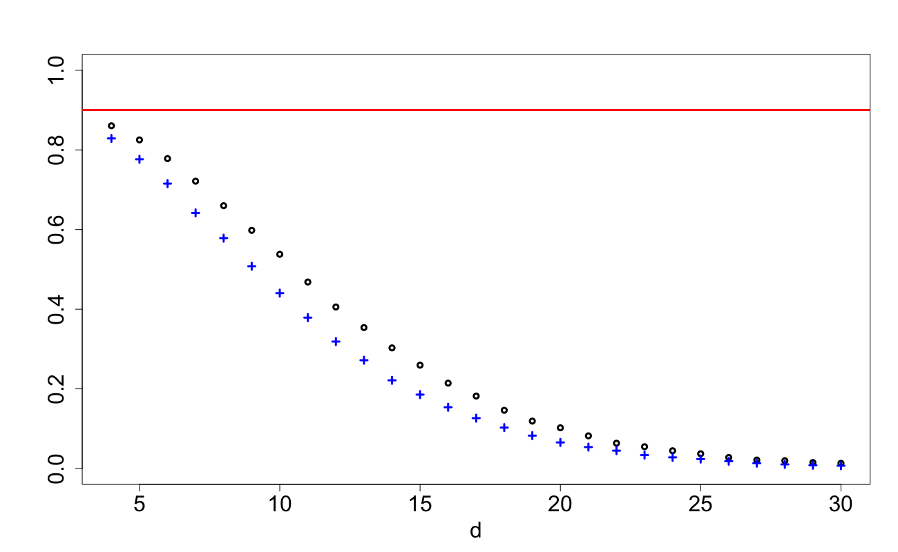
Figure 1: Covering proportions using the
asymptotic radius; $n=1000,\;10000$.

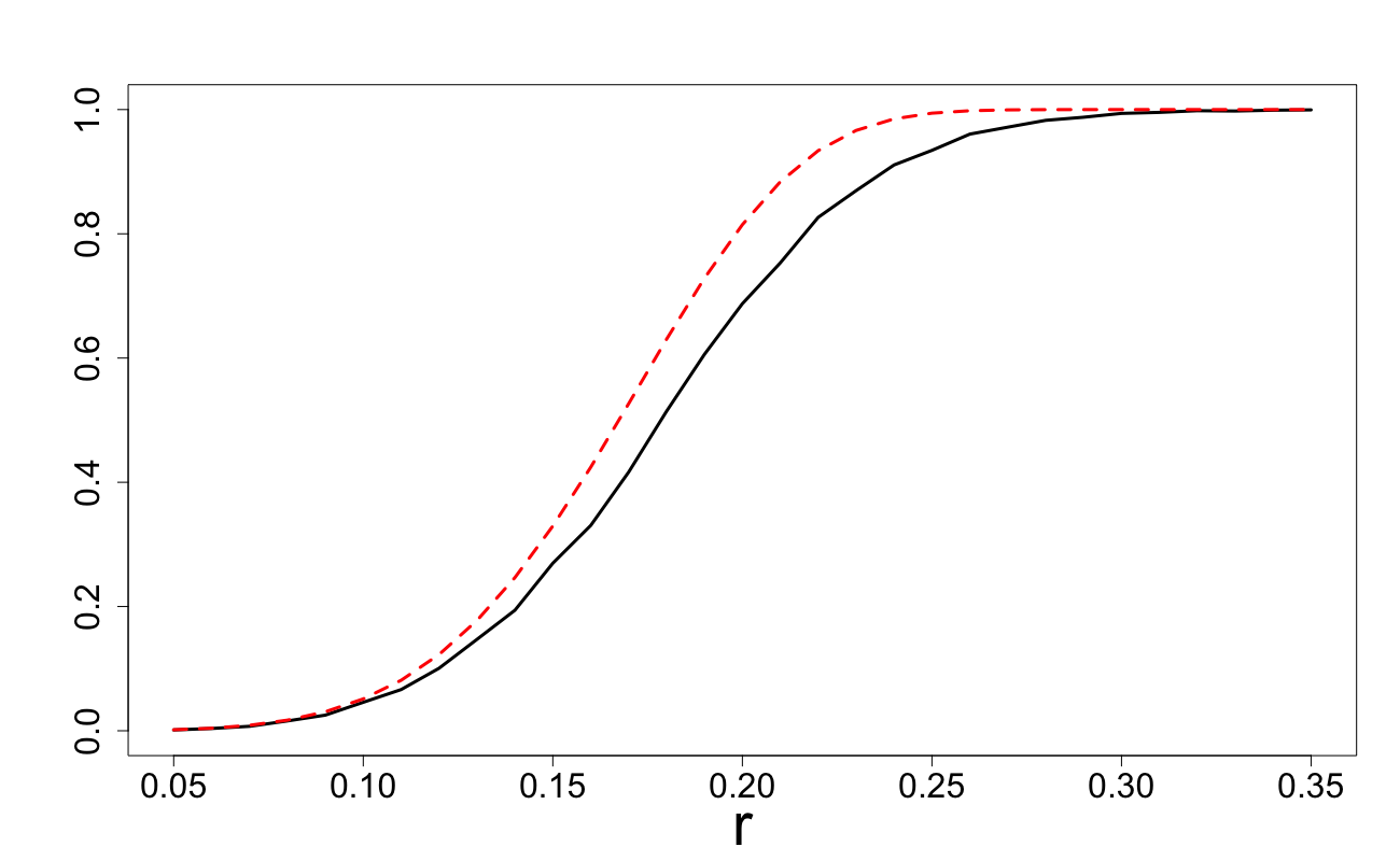
Figure 2: $F_{d}(r,X_{n})$ and $F(n^{1/d}V_{d}^{1/d}r)$ as functions of $r$; $d=5$ and $n=1000$

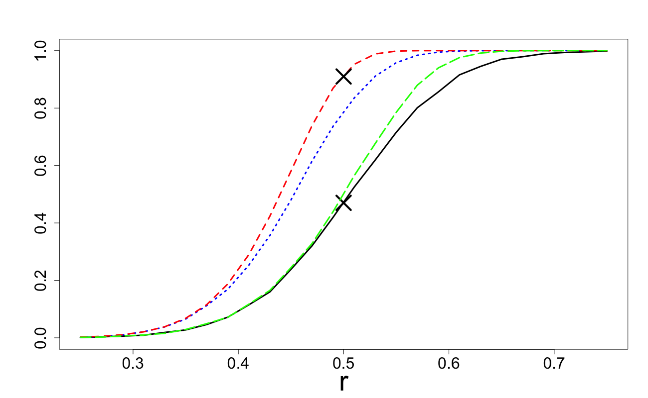
Figure 3: $d=10,\;n=1000.$

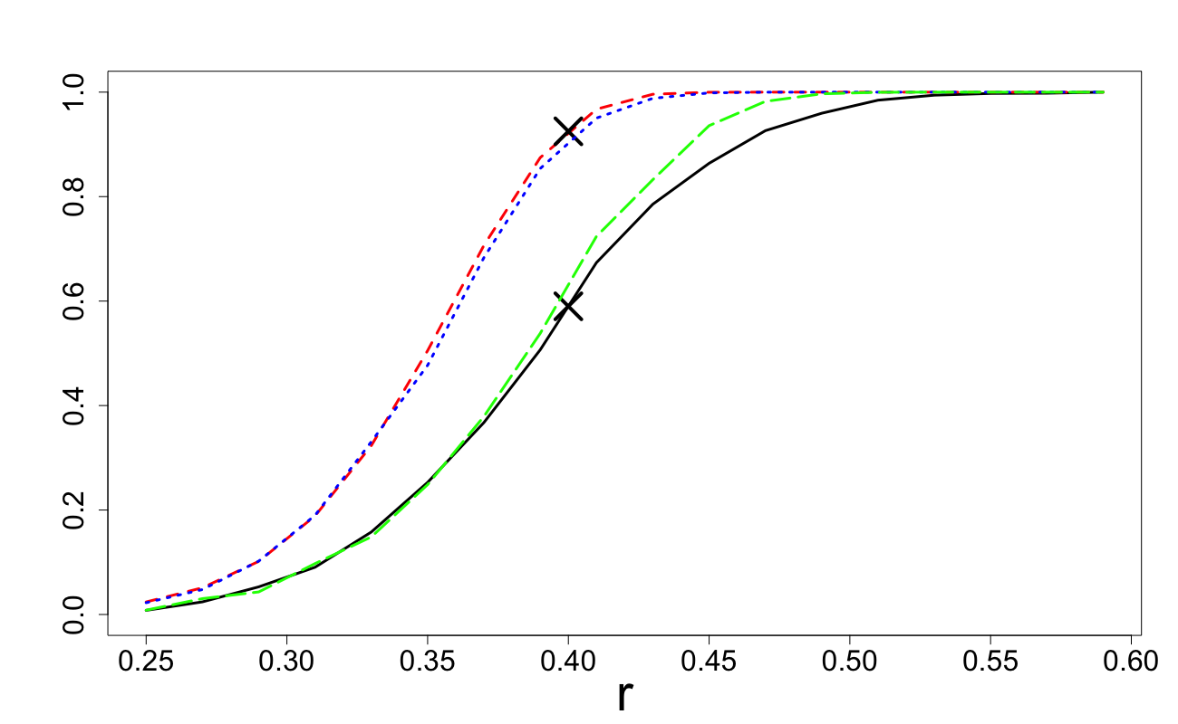
Figure 4: $d=10,\;n=10000.$

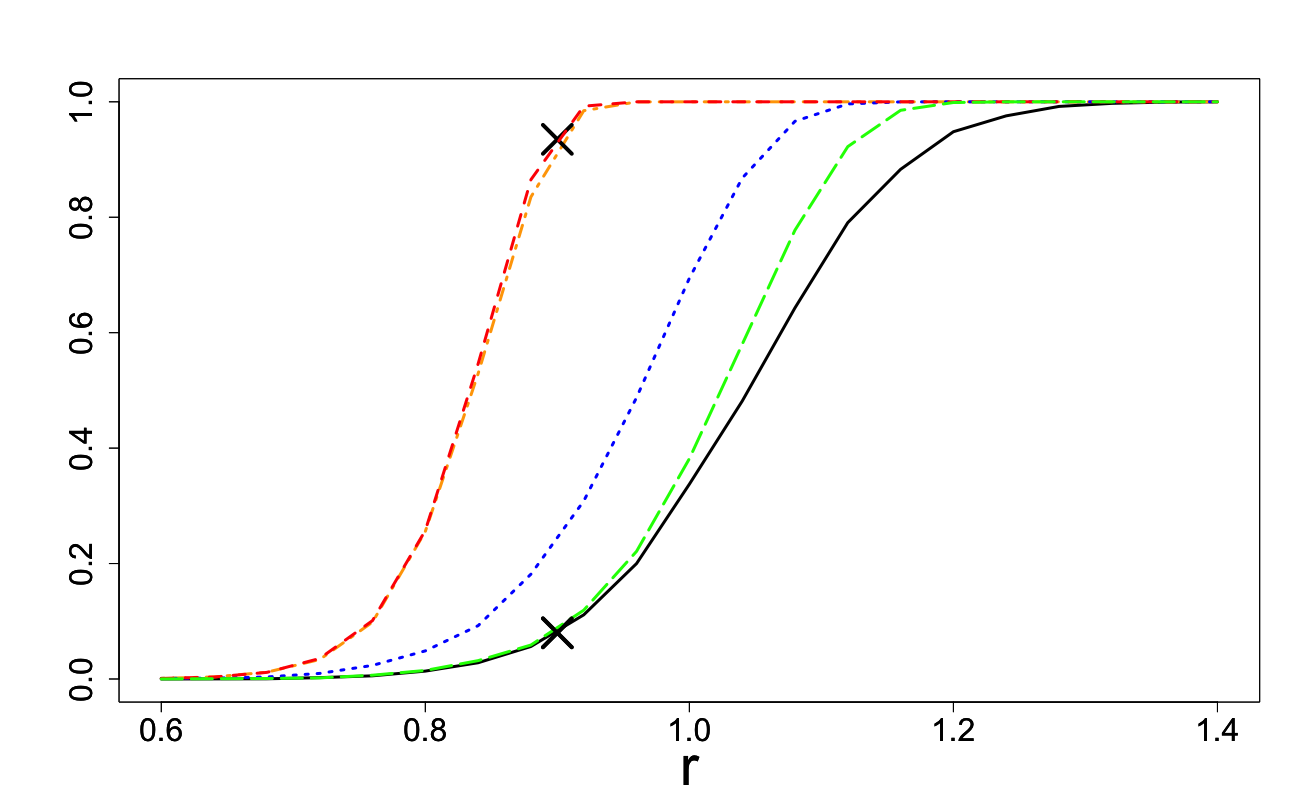
Figure 5: $d=20,\;n=1000.$

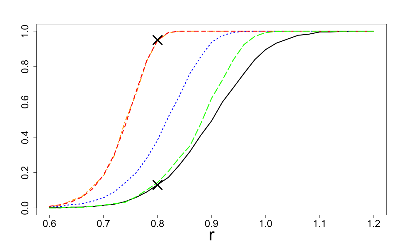
Figure 6: $d=20$, $n=10000.$

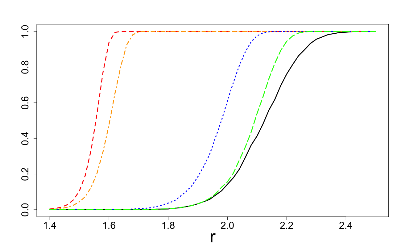
Figure 7: $n=1000,d=50$

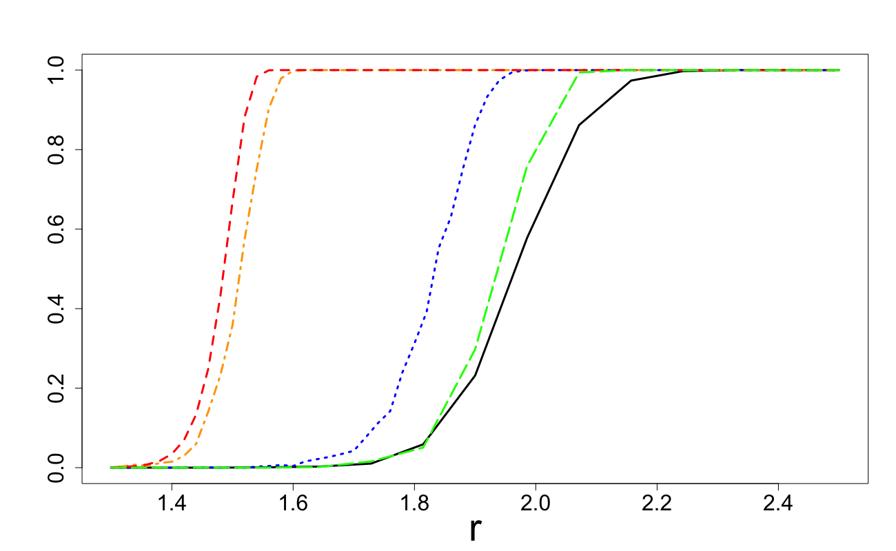
Figure 8: $n=10,000,d=50$

In Figures 10 and 10 we use $d=10$, $d=20$ and the values of $r$ corresponding to the crosses in Figures 4 and 6. In these figures, we depict the distribution of intersection a random point has with the cube normalised by the volume of the ball $r^{d}V_{d}$; that is, we plot the density of the r.v. $\kappa_{U}=\mathbb{P}_{X}\left\{\|U-{X}\|\leq r\right\}/(r^{d}V_{d})$, where both $U$ and $X$ have uniform distribution on $[0,1]^{d}$. The importance of these two figures is another illustration of inadequacy of the key assumption behind (2.6), which can be formulated as the assumption that the distribution of density of the r.v. $\kappa_{U}$ is very close to the delta-measure concentrated at one. This assumption is indeed reasonably adequate if $r$ can be chosen small enough. However, as Figure 10 and especially Figure 10 illustrate, even for relatively large values of $n$ the required values of $r$ are not small enough for this to hold even approximately. Note that in the derivation of the asymptotic values of $n_{\gamma}=n_{\gamma}^{\rm as}$ in (2.6) we use the value 1 rather than the random variables $\kappa_{U}$ with the densities shown in Figures 10,10.

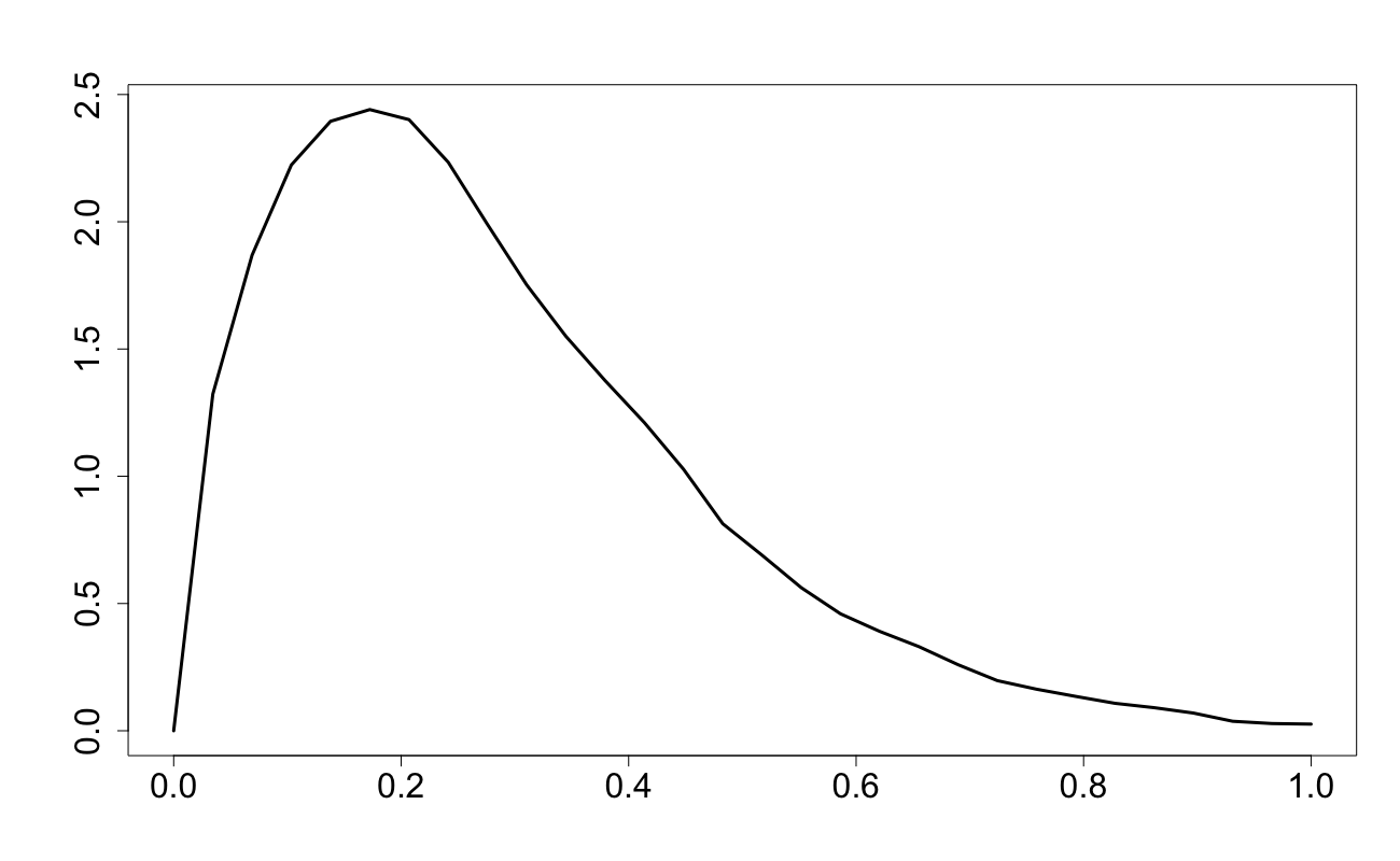
Figure 9: Density of r.v. $\kappa_{U}$; $d=10,r=0.5$

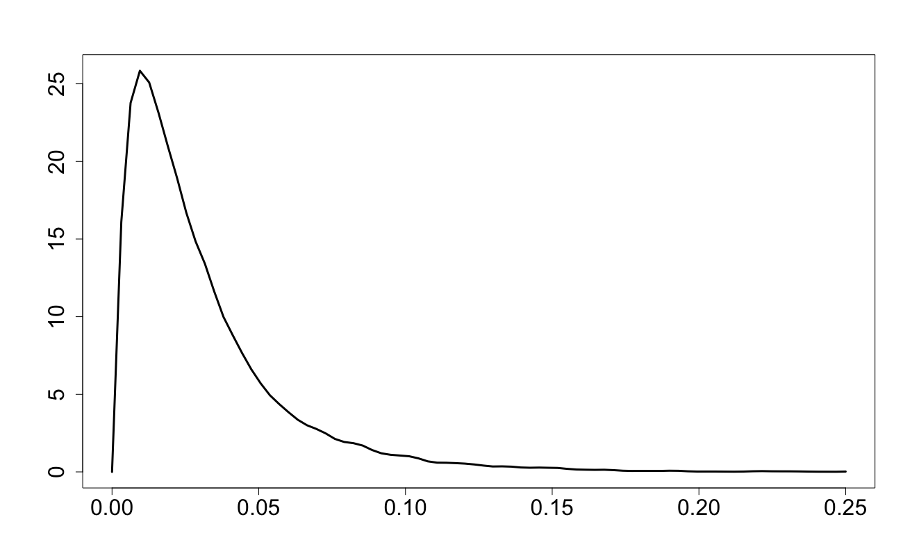
Figure 10: Density of r.v. $\kappa_{U}$; $d=20,r=0.9$

4 Modification of sampling schemes and non-uniform distribution of the target

In Section 3, we have used the principal sampling scheme where points $x_{j}$ in $X_{n}=\{x_{1},\ldots,x_{n}\}$ are i.i.d. uniform on ${\cal X}=[0,1]^{d}$. In Section 4.1 we study a modification of this scheme where $x_{j}\in X_{n}$ are i.i.d. uniform random points in a smaller $\delta$-cube $C_{\delta}=[1/2-\delta/2,1/2+\delta/2]^{d}$ with $0<\delta<1$. In Section 4.2 we investigate the effect of replacing random points by points from a low-discrepancy sequence. The choice of a specific low-discrepancy sequence has very little impact on the results and we present the results for Sobol sequence only. In Section 4.3 we will investigate the effect of replacement of the uniform distribution of the target $x_{*}\in[0,1]^{d}$ by a bowl-shaped distribution such as the product of arcsine distributions on $[0,1]$.

4.1 Points $x_{j}$ are i.i.d. uniformly distributed on $C_{\delta}$

In this section we demonstrate the $\delta$-effect, which manifests that in high dimensions sampling in a cube $C_{\delta}$ with suitable $0<\delta<1$ leads to a much more efficient covering scheme than sampling within the whole cube $[0,1]^{d}$. Note that the $\delta$-effect is not obvious being completely unknown in the literature on stochastic global optimization and perhaps in literature on global optimization in general. All existing literature recommends space-filling in the whole set $X$ and not in its subset. Moreover, there are recommendations in literature (see, for example, Janson (1986); Tsvetkov and Krymov (2022)) of choosing more points closer to the boundary of the cube rather than purely uniformly in order to improve space-filling properties of random points.

In Figures 12–14, for different values of $d$ and $n$ we plot $F_{d}(r,X_{n})$ as a function of $\delta$. For each $d$ and $n$, the value of $r$ has been chosen such that $\max_{0\leq\delta\leq 1}F_{d}(r,X_{n})=0.9$; these values of $r$ (along with optimal values of $\delta$, in brackets) can be obtained from Table 1. In these figures, the values of $F_{d}(r,X_{n})$ for $n=1000,10000,100000$ are shown with a solid black line, dashed blue line and dotted green line respectively. These figures demonstrate the ‘$\delta$-effect’ formulated as the second main message in Introduction. These figures also clearly demonstrate that despite sampling uniformly in the cube $[0,1]^{d}$ is asymptotically optimal, for large $d$ it is always a poor strategy, which can be substantially improved.

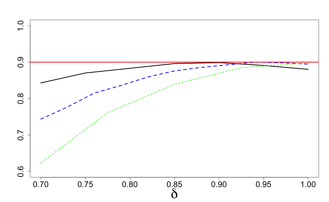
Figure 11: $d=10;\;n=1000,10000,100000$.

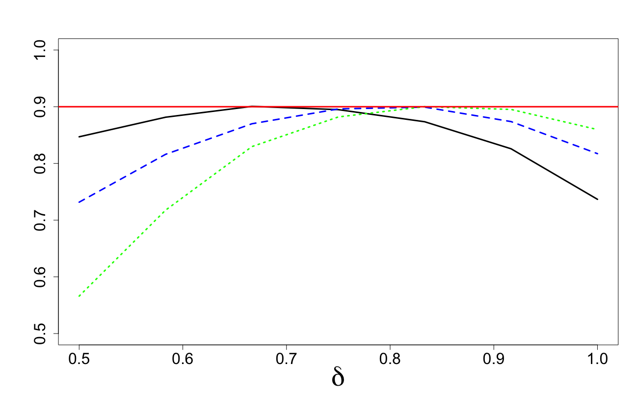
Figure 12: $d=20;\;n=1000,10000,100000$.

Figure 13: $d=50;\;n=1000,10000,100000$.

Figure 14: $d=10,n=1000$: Jensen’s bound with $\delta=1$ and $\delta=0.5$.

The discussion of Jensen’s bounds given in Section 3.2 still apply to the case of $X_{n}$ sampled uniformly within $\delta$-cube $C_{\delta}$. The only adjustment that needs to be made to the results of Section 3.2 is to let $X$ be a uniform random vector in $C_{\delta}$ and not $[0,1]^{d}$. In Figure 14, we depict the Jensen’s lower bound given in (3.9) for $X$ uniform in $[0,1]^{d}$ and for $X$ uniform in the $\delta$ cube $[{1/4,3/4}]^{d}$ (so that $\delta=0.5$). We see that the lower bound for $X_{n}$ sampled within the $\delta$-cube is larger than $X_{n}$ sampled from the whole cube. This further supports the conclusion that for $n$ not astronomically large, the ‘$\delta$-effect’ should always be considered.

In Table 1, for $X_{n}$ chosen uniformly in the cube $[0,1]^{d}$ and $X_{n}$ chosen uniformly in the $\delta$-cube, we tabulate the values of $r_{n,1-\gamma}$ with $\gamma=0.1$ for different $d$ and $n$. In the columns labeled $\delta$-cube, the values in the brackets correspond to the approximately optimal values of $\delta$. We can see that for small $d$, the $\delta$-effect is very small (since $n$ is relatively large in these dimensions). For larger dimensions, the $\delta$-effect is very prominent.

	$n=100$		$n=1,000$		$n=10,000$		$n=100,000$
	$[0,1]^{d}$	$\delta$-cube	$[0,1]^{d}$	$\delta$-cube	$[0,1]^{d}$	$\delta$-cube	$[0,1]^{d}$	$\delta$-cube
$d=5$	0.41	0.40 (0.9)	0.24	0.24 (1.0)	0.24	0.29 (1.0)	0.09	0.089 (1.0)
$d=10$	0.81	0.78 (0.7)	0.61	0.60 (0.9)	0.46	0.46 (1.0)	0.36	0.360 (1.0)
$d=15$	1.13	1.04 (0.6)	0.91	0.88 (0.8)	0.76	0.74 (0.9)	0.62	0.619 (0.9)
$d=20$	1.38	1.25 (0.5)	1.17	1.11 (0.7)	1.01	0.97 (0.8)	0.87	0.855 (0.9)
$d=25$	1.60	1.42 (0.5)	1.39	1.30 (0.6)	1.23	1.18 (0.8)	1.09	1.060 (0.8)
$d=50$	2.46	2.07 (0.4)	2.26	1.98 (0.5)	2.10	1.90 (0.5)	1.96	1.790 (0.6)

Table 1: Values for $r_{n,1-\gamma}$ with $\gamma=0.1$.

In Tables 2–3, we consider an equivalent reformulation of the results of Table 1. In these tables, for a given $r$ we specify the value of $n_{\gamma}$, with $\gamma=0.1$, for $X_{n}$ chosen uniformly in the cube $[0,1]^{d}$ and $X_{n}$ chosen uniformly in the $\delta$-cube. We also include the approximation based on the the asymptotic arguments leading to (2.6). We see that in high dimensions, the requirement of $r$ being small enough for (2.6) to provide sensible approximations requires $n$ to be extremely large. Such large values of $n$ are impractical.

$r$	0.9	0.95	1	1.05	1.1	1.15
$n_{\gamma}$ with $\delta=1$	54,000	25,000	10,800	4,600	2,700	1,300
$n_{\gamma}$ with $\delta=\delta^{*}$	40,000 (0.8)	15,000 (0.8)	6,300 (0.8)	2,700 (0.7)	1,100 (0.7)	500 (0.7)
$n_{\gamma}$ from (2.6)	734	249	89	34	13	5

Table 2: Values of $n_{\gamma}$: $d=20,\gamma=0.1.$

$r$	2	2.05	2.1	2.15	2.2	2.25	2.3
$n_{\gamma}$ with $\delta=1$	50,000	21,000	10,000	5,000	2,200	1,200	600
$n_{\gamma}$ with $\delta=\delta^{*}$	700 (0.4)	200 (0.4)	50 (0.3)	12 (0.2)	2 (0.1)	NA	NA
$n_{\gamma}$ from (2.6)	0	0	0	0	0	0	0

Table 3: Values of $n_{\gamma}$: $d=50,\gamma=0.1.$

4.2 Points $x_{j}$ are taken from a low-discrepancy sequence

Figures 16-16 are extended versions of Fig. 2. Here we plot $F_{d}(r,X_{n})$ as a function of $d$, where the radius is fixed from (3.5) with $\gamma=0.1$ (the line $1-\gamma$ is depicted by a red solid line). For $X_{n}$ chosen uniformly in the cube $[0,1]^{d}$, we depict $F_{d}(r,X_{n})$ with blue plusses. For $X_{n}$ chosen from a Sobol sequence in the whole cube $[0,1]^{d}$, we use orange triangles. When the points in $X_{n}$ are uniform i.i.d. within the $\delta$-cube with optimal $\delta$ we use green crosses. Finally, when points in $X_{n}$ are chosen from a Sobol sequence within the same $\delta$-cube we use purple diamond. Figures 16 and 16 illustrate two new key messages along with the message discussed in Figure 2. Firstly, the use of low-discrepancy sequences seem to produce slightly better results in comparison to random choice of points for small dimensions but in higher dimensions the use of low-discrepancy sequences (in our case, Sobol sequences) produces results that are almost equivalent to random sampling uniformly either in $[0,1]^{d}$ or in the optimally chosen $\delta$-cube. Secondly, in large dimensions sampling from a suitable $\delta$-cube greatly outperforms the other schemes considered here being still far from the asymptotic results. These messages are further supported in Figures 18 and 18. Here we plot the asymptotic approximation $F_{n}(r)$ from Lemma 1 (dashed red) and $F_{d}(r,X_{n})$ as a function of $r$ for the following choices of $X_{n}$: random in the cube $[0,1]^{d}$ (blue line with plusses), chosen from a Sobol sequence in $[0,1]^{d}$ (orange line with triangles), random in the $\delta$-cube with optimal delta (green line with crosses), chosen from a Sobol sequence within the same $\delta$-cube (purple line with diamonds). We see that in Figure 18 for $d=10$, the Sobol sequence is slightly advantageous to the random uniform on the whole cube and $\delta$-cube for most interesting values of $\gamma$. Choosing $X_{n}$ as uniform within the $\delta$-cube produces better coverings than with Sobol’s points in $[0,1]^{d}$ for most values of $\gamma$, but slightly worse for small $\gamma$. This slight advantage of the Sobol sequence in $[0,1]^{d}$ and in the $\delta$-cube diminishes in the case $d=20$ shown in Figure 18.

To further study the similarities in performance between $X_{n}$ chosen randomly in the $\delta$-cube with optimal $\delta$ and $X_{n}$ chosen from a Sobol sequence within the same $\delta$-cube, in Figures 20-20 we plot the ratio of the c.d.f.’s $F_{d}(r,X_{n,U})/F_{d}(r,X_{n,S})$ across different $d$. The subscript $U$ and $S$ respectively differentiate between $X_{n}$ chosen randomly in the $\delta$-cube with optimal $\delta$ and $X_{n}$ chosen from a Sobol sequence within the same $\delta$-cube. For each value of $d$, $r$ is chosen so that $\max_{0\leq\delta\leq 1}F_{d}(r,X_{n,U})=0.9$.

Figure 15: overing using the asymptotic radius
with Sobol and $\delta$-cube points: $n=2^{10}$.

Figure 16: Covering using the asymptotic radius
with Sobol and $\delta$-cube points: $n=2^{13}$.

Figure 17: Sobol and $\delta$-cube points versus
the asymptotic covering: $d=10,n=1024$.

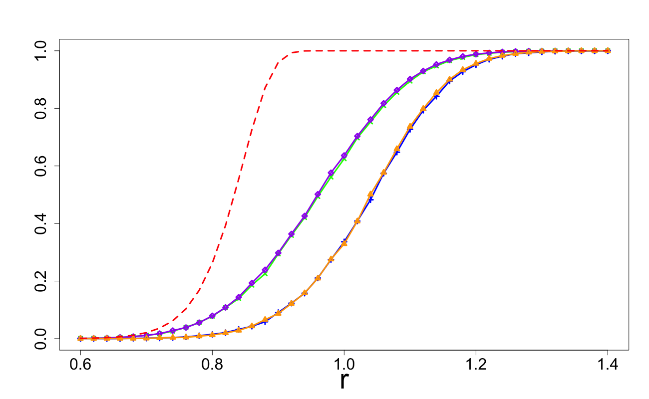
Figure 18: Sobol and $\delta$-cube points versus
the asymptotic covering: $d=20,n=1024$.

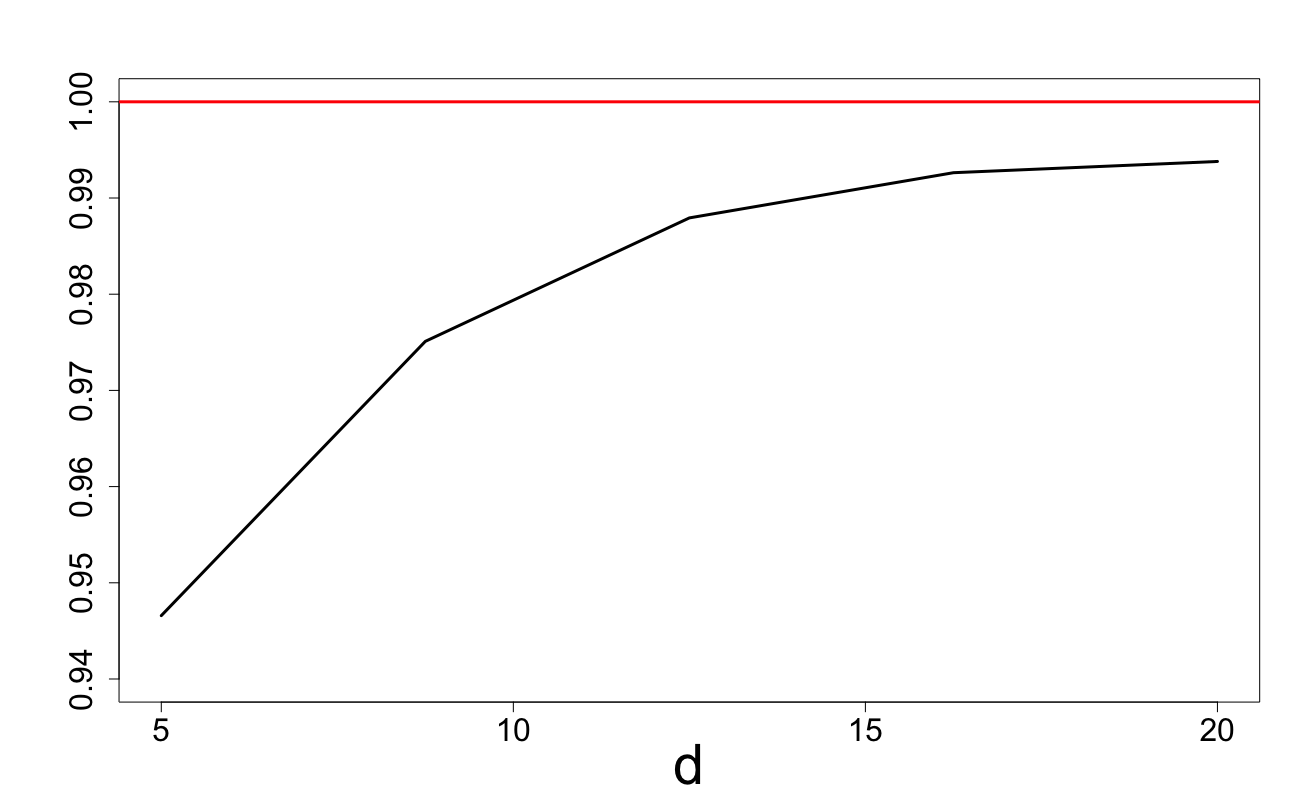
Figure 19: Efficiency of Sobol’s points, $n=2^{10}$.

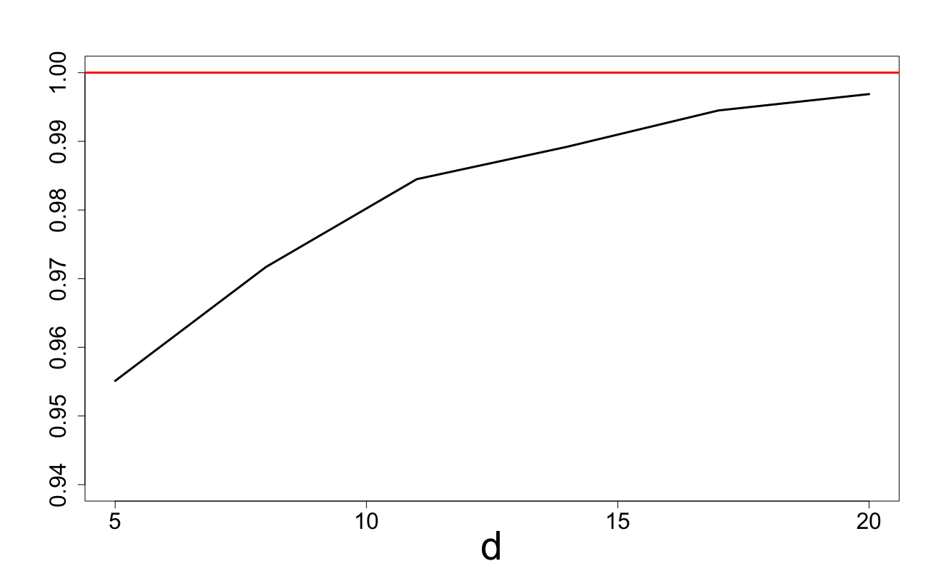
Figure 20: Efficiency of Sobol’s points, $n=2^{13}$.

4.3 Non-uniform prior distribution for the target

In this section, we explore the effect a non-uniform prior distribution for $x_{*}\in{\cal X}$ has on the conclusions above formulated for the case of uniform distribution. We will assume that each component of $x_{*}$ has independent components distributed according to the following symmetric beta distribution with density:

$$p_{\alpha}(t)=\frac{t^{\alpha-1}[1-t]^{\alpha-1}}{\mbox{Beta$(\alpha,\alpha)$}}\,,\text{ for some }\alpha>0\,.$$

If $\alpha=1$, the density $p_{\alpha}(t)$ is uniform on $[0,1]$ while for $0<\alpha<1$ this density is U-shaped. In most cases below we choose the arcsine density $p_{0.5}(t)$.

We then select the distribution of random points $x_{j}\in X_{n}$ to have similar shape but constrained to the $\delta$-cube. More precisely, we assume that $x_{j}$ have independent components with the density

$$p_{\alpha,\delta}(t)=\frac{2\cdot(2\delta)^{1-2\alpha}}{\mbox{Beta$(\alpha,\alpha)$}}[\delta^{2}-(2t-1)^{2}]^{\alpha-1}\,,\;\;\frac{1-\delta}{2}<t<\frac{\delta+1}{2}\,,\text{ for some }\alpha>0\;\;{\rm and}\;0\leq\delta\leq 1.$$

In the case $\alpha=1$, the points $x_{j}$ have uniform distribution on the cube $C_{\delta}$.

Figures 22–22 are similar to Figures 12–14, but with the key difference of assuming a non-uniform prior distribution for $x_{*}$. For different values of $d$ and $n$ and for $\alpha=0.5$, we plot $F_{d}(r,X_{n})$ as a function of $\delta$. For each $d$ and $n$, the value of $r$ has been chosen so that $\max_{0\leq\delta\leq 1}F_{d}(r,X_{n})=0.9$. In these figures, the values of $F_{d}(r,X_{n})$ for $n=1000,10000,100000$ are shown with a solid black line, dashed blue line and dotted green line respectively. Figures 24-24 are similar to Figures 22–22, but with varying values of $\alpha$ and fixed $n=10000$. In these figures, we selected $\alpha=0.25$ (dashed dark green), $\alpha=0.5$ (dotted purple), $\alpha=0.75$ (dot-dashed grey) and $\alpha=1$ which gives the uniform distribution (solid black). Figures 22–22 clearly demonstrate that the ‘$\delta$-effect’ is still significant in this non-uniform setting.

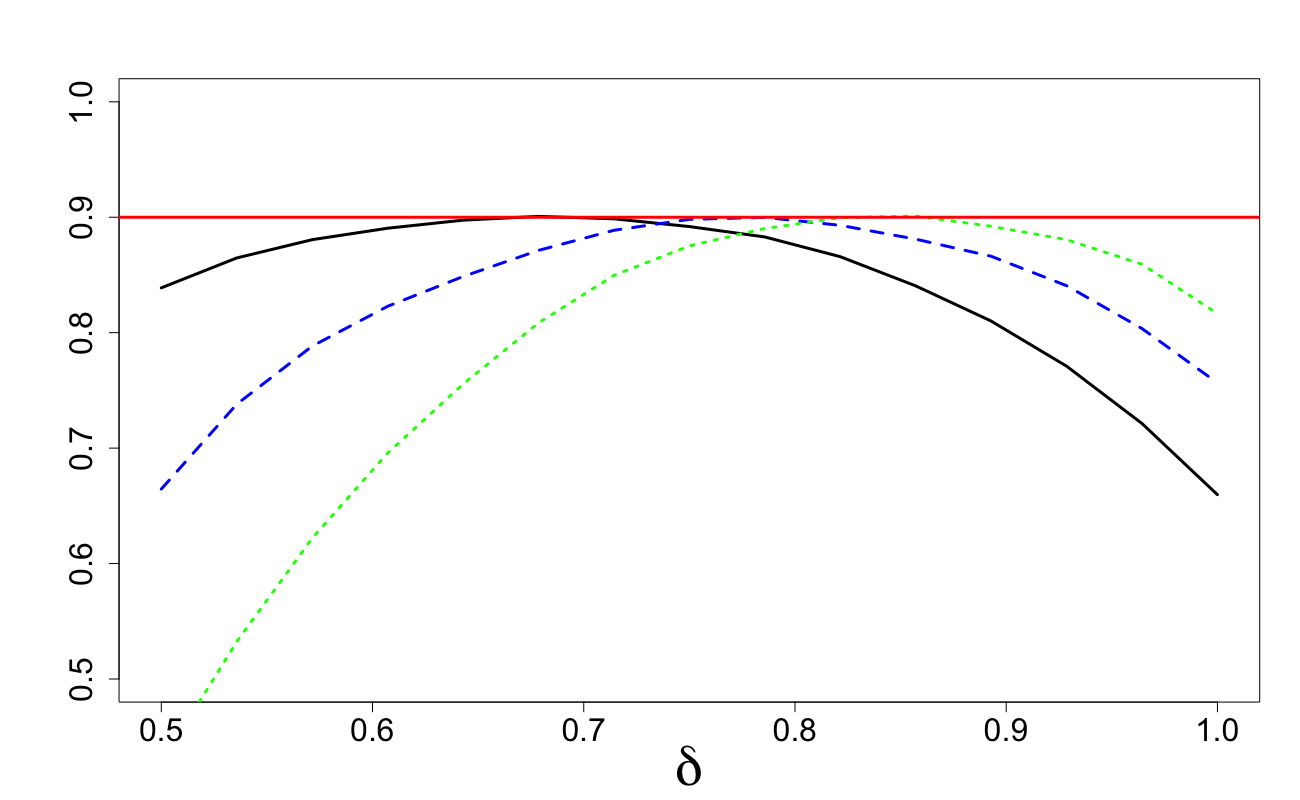
Figure 21: $d=20$ and $\alpha=0.5$ with
$n=1000,10000,100000$.

Figure 22: $d=50$ and $\alpha=0.5$ with
$n=1000,10000,100000$.

Figure 23: $d=20,n=10000$ and
$\alpha=0.25,0.5,0.75,1$.

Figure 24: $d=50,n=10000$ and
$\alpha=0.25,0.5,0.75,1$.

5 Intersection of one ball with the cube

As a result of (3.6), our main quantity of interest in this section will be the probability

$$P_{U,\delta,r}:=\mathbb{P}_{{}_{X}}\left\{\|U\!-\!X\|\!\leq\!{r}\right\}\!=\!\mathbb{P}_{{}_{X}}\left\{\|U\!-\!X\|^{2}\leq{r^{2}}\right\}\!=\!\mathbb{P}\left\{\sum_{j=1}^{d}(u_{j}\!-\!x_{j})^{2}\leq{r}^{2}\right\}\;\;$$ (5.1)

in the case when $X$ has the uniform distribution on the $\delta$-cube $[1/2-\delta/2,1/2+\delta/2]^{d}$ and ${U=(u_{1},\ldots,u_{d})\in\mathbb{R}^{d}}$ is fixed. The case of $\delta=1$ will be directly applicable to Section 3.2. Because of the results of Section 3.2, we will bear in mind two typical choices of $U$ will be $U=\bm{1/2}$ and $U=\bm{3/4}$ but will formulate results for general $U$.

For fixed $u\in\mathbb{R}^{d}$, consider the r.v. $\eta_{u,\delta}=(z-u)^{2}$, where $z$ has density

$$p_{\delta}(t)=1/\delta\,,\;\;(1-\delta)/2<t<(1+\delta)/2\,,\text{ for some }0\leq\delta\leq 1.$$ (5.2)

The first three central moments of $\eta_{u,\delta}$ are:

$$\mu_{u}^{(1)} = \mathbb{E}\eta_{u,\delta}=\left(u-\frac{1}{2}\right)^{2}+\frac{{{\delta}}^{2}}{12}\,,$$ (5.3)

$$\mu_{u}^{(2)} = {\rm var}(\eta_{u,\delta})={\frac{\delta^{2}}{3}}\left[\left(u-\frac{1}{2}\right)^{2}+{\frac{{{\delta}}^{2}}{60}}\right]\,,$$ (5.4)

$$\mu_{u}^{(3)} = \mathbb{E}\left[\eta_{u,\delta}-\mu_{u}^{(1)}\right]^{3}={\frac{4{{\delta}}^{4}}{15}}\left[\left(u-\frac{1}{2}\right)^{2}+{\frac{{{\delta}}^{2}}{252}}\right]\,.$$ (5.5)

Then for given $U=(u_{1},\ldots,u_{d})\in\mathbb{R}^{d}$, consider the random variable

$$\|U-X\|^{2}=\sum_{i=1}^{d}\eta_{u_{i},\delta,\alpha}=\sum_{j=1}^{d}(u_{j}-x_{j})^{2}\,,$$

where we assume that $X=(x_{1},\ldots,x_{d})$ is a random vector with i.i.d. components $x_{i}$ with density (5.2). From (5.3), its mean is

$$\mu=\mu_{d,\delta,U}:=\mathbb{E}\|U-X\|^{2}=\|U-\bm{1/2}\|^{2}+\frac{{d{\delta}}^{2}}{12}\,.$$

Using independence of $x_{1},\ldots,x_{d}$ and (5.4), we obtain

$${\sigma}_{d,\delta,U}^{2}:={\rm var}(\|U-X\|^{2})={\frac{\delta^{2}}{3}}\left[\|U-\bm{1/2}\|^{2}+{\frac{{d{\delta}}^{2}}{60}}\right]\,,$$

and from independence of $x_{1},\ldots,x_{d}$ and (5.5) we get

$${\mu}_{d,\delta,U}^{(3)}:=\mathbb{E}\left[\|U-X\|^{2}-\mu\right]^{3}=\sum_{j=1}^{d}\mu_{u_{j}}^{(3)}={\frac{\,{{\delta}}^{4}}{15}}\left[\|U-\bm{1/2}\|^{2}+{\frac{{d{\delta}}^{2}}{252}}\right]\,.\;\;\;\;\;\;$$ (5.6)

If $d$ is large enough then the conditions of the CLT for $\|U-X\|^{2}$ are approximately met and the distribution of $\|U-X\|^{2}$ is approximately normal with mean $\mu_{d,\delta,U}$ and variance ${\sigma}_{d,\delta,U}^{2}$. That is, we can approximate the probability $P_{U,\delta,r}=\mathbb{P}_{{}_{X}}\left\{\|U\!-\!X\|\!\leq\!{r}\right\}$ by

$$P_{U,\delta,r}\!\cong\Phi\left(\frac{{r}^{2}-\mu_{d,\delta,U}}{{\sigma}_{d,\delta,U}}\right)\,,$$ (5.7)

where $\Phi(\cdot)$ is the c.d.f. of the standard normal distribution:

$$\Phi(t)=\int_{-\infty}^{t}\varphi(v)dv\;\;{\rm with}\;\;\varphi(v)=\frac{1}{\sqrt{2\pi}}e^{-v^{2}/2}\,.$$

The approximation (5.7) has acceptable accuracy if the probability $P_{U,\delta,r}$ is not very small; for example, it falls inside a $2\sigma$-confidence interval generated by the standard normal distribution.

To improve on the usual CLT approximation, we use Edgeworth-type expansion in the CLT for sums of independent non-identically distributed r.v. by V.Petrov, see Petrov (1975):

$$P\left(\frac{\|U-X\|^{2}-\mu_{d,\delta,U}}{\sigma_{d,\delta,U}}\leq t\right)=\Phi(t)+\sum_{\nu=1}^{\infty}\frac{Q_{\nu,d}(t)}{d^{\nu/2}}\,,$$ (5.8)

where

$$Q_{\nu,d}(t)=-\varphi(t)\sum H_{\nu+2s-1}(t)\prod_{m=1}^{\nu}\frac{1}{k_{m}!}\left(\frac{\lambda_{m+2,d}}{(m+2)!}\right)^{k_{m}}\,,$$

$$\lambda{}_{\nu,d}=\frac{d^{(\nu-2)/2}}{\sigma_{d,\delta,U}^{\nu}}\sum_{j=1}^{d}\gamma_{\nu,j}\,$$

$\gamma_{\nu,j}$ is the cumulant of order $\nu$ at $(u_{j}-x_{j})^{2}$, $H_{m}$ is the Chebyshev-Hermite polynomial of degree $m$ and the summation is carried out over all non-negative integer solutions of the equation

$$k_{1}+2k_{2}+\cdots+\nu k_{\nu}=\nu$$

$$s=k_{1}+k_{2}+\cdots+k_{\nu}\,.$$

The partition function $p(\nu)$ provides the number of possible partitions of a non-negative integer $\nu$ and therefore at each value of $\nu$ provides the number of terms in the summation. The sequence has the generating function

$$\sum_{\nu=0}^{\infty}p(\nu)x^{\nu}=\prod_{k=1}^{\infty}\left(\frac{1}{1-x^{k}}\right);$$

the first few values are: 1, 1, 2, 3, 5, 7, 11, 15, 22, 30, 42, 56, 77, 101. The first few terms in the summation (including Hermite polynomials) are provided in (Petrov, 1995, p. 139).

In the case of $U=\bm{1/2}$ or $U=\bm{3/4}$, the random variables $(u_{j}-x_{j})^{2}$ will be i.i.d. For this case $\lambda_{\nu,d}$ does not depend on $d$ and thus we have the slight simplification $\lambda{}_{\nu,d}=\lambda{}_{\nu}=\gamma_{\nu}/\sigma_{d,\delta,U}^{\nu}$.

In Figures 26–30, we plot $P_{U,1,r}$ for $U=\bm{1/2}$ and $U=\bm{3/4}$ as a function of $r$ with a solid black line. In these figures, we demonstrate the accuracy of approximation (5.7) with a dashed blue line. With a dot-dashed red line, we plot the accuracy of an approximation obtained by taking one additional term in the expansion given in (5.8); this requires use of the third central moment given in (5.6). We can see that overall, for $d=10$ and $d=20$, the approximations are fairly accurate. However, when considering covering by $n$ balls it is more important to focus on the lower tail. Figures 26, 28, 30 and 30 demonstrate that taking one additional term in the Petrov’s expansion (5.8) produces a significant improvement in accuracy.

Figure 25: $d=10,U=\bm{1/2}$.

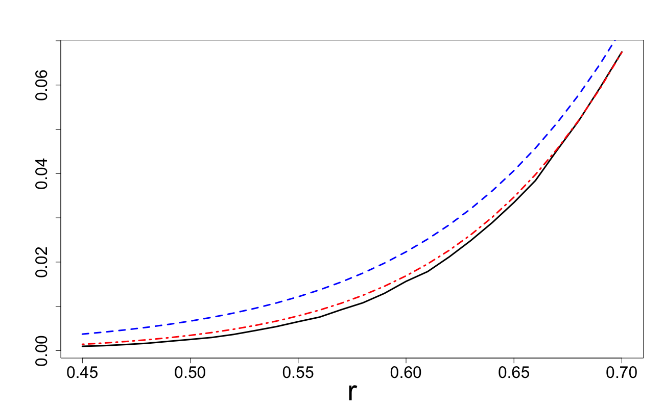
Figure 26: $d=10,U=\bm{1/2}$.

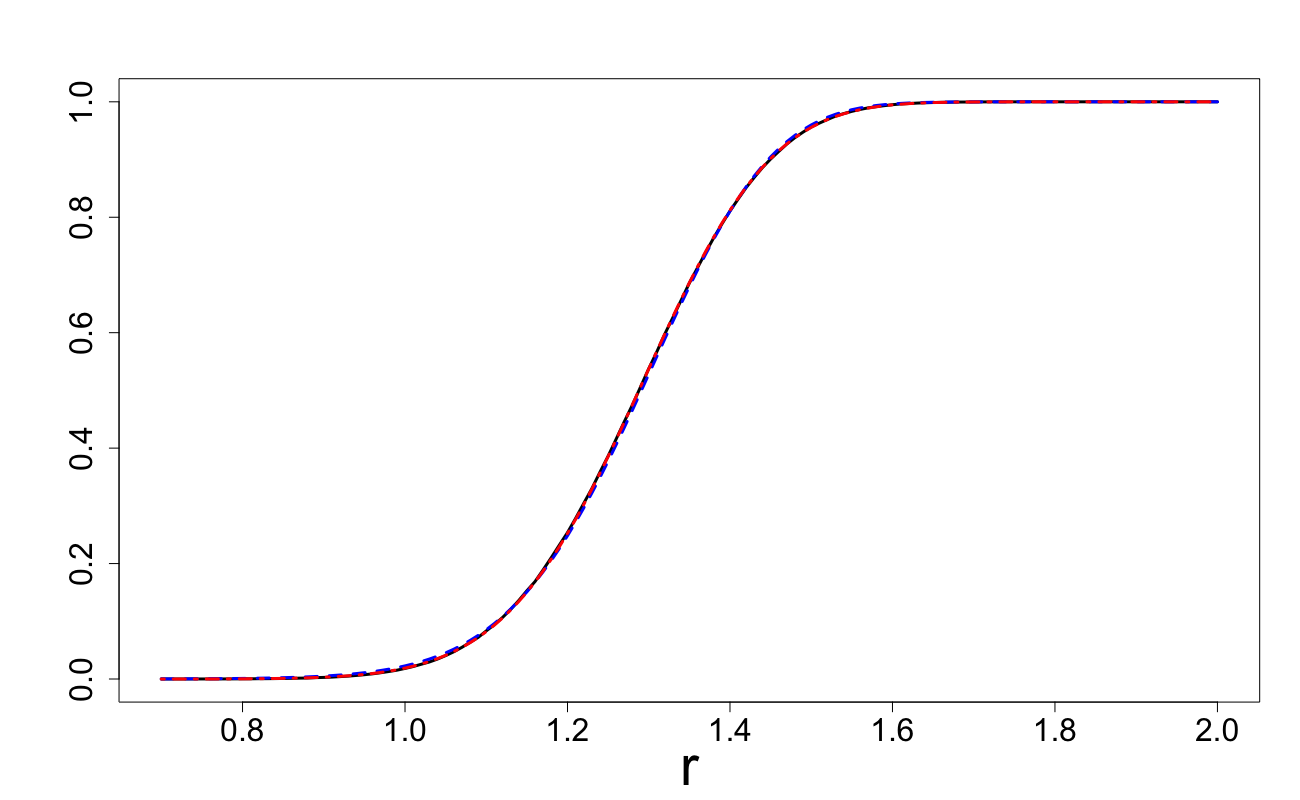
Figure 27: $d=20,U=\bm{1/2}$.

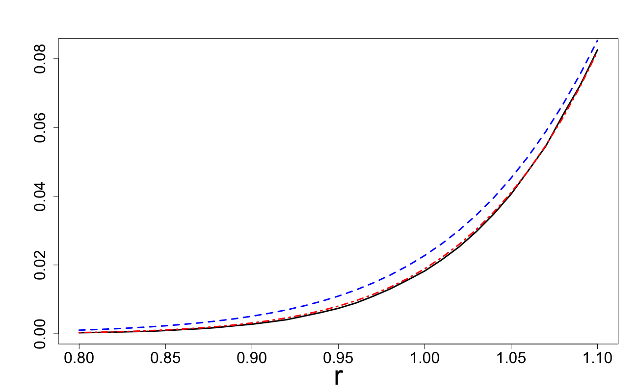
Figure 28: $d=20,U=\bm{1/2}$.

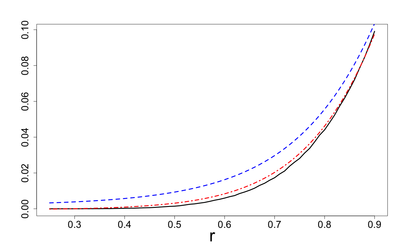
Figure 29: $d=10,U=\bm{3/4}$.

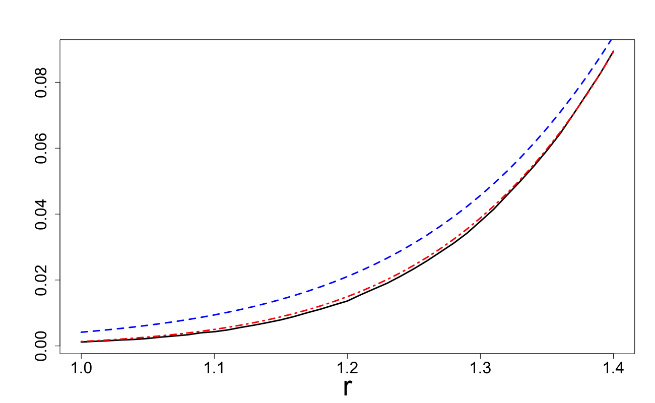
Figure 30: $d=20,U=\bm{3/4}$.

6 Conclusions

We have considered continuous global optimization problems, where the feasible region ${\cal X}$ is a compact subset of $\mathbb{R}^{d}$. As a strategy for exploration, we have mostly considered sampling of i.i.d. random points either in ${\cal X}$ or a suitable subset of ${\cal X}$.

We have distinguished between between ‘small’, ‘medium’ and ‘high’ dimensional problems depending on the following relations between $d$ and $n_{\max}$ (which is the maximum possible number of points available for space exploration):

• small dimensions: $n_{\max}\gg 2^{d}$ (roughly, $d<10$);

• medium dimensions: $n_{\max}$ is comparable to $2^{d}$ (roughly, $10\leq d\leq 20$);

• high dimensions: $n_{\max}\ll 2^{d}$ (roughly, $d>20$).

We only considered the situations (M) and (H), where we have demonstrated the following effects: (i) the actual convergence of randomized exploration schemes is much slower than that given by the classical estimates, which are based on the asymptotic properties of random points; (ii) the usually recommended space exploration schemes are practically inefficient as the asymptotic regime is unreachable. In particular, we have shown: (ii-a) uniform sampling on entire ${\cal X}$ is much less efficient than uniform sampling on a suitable subset of ${\cal X}$, and (ii-b) the effect of replacement of random points by a low-discrepancy sequence is very small so that using low-discrepancy sequences and other deterministic constructions does not lead to significant improvements (unless the number of evaluation points $n=n_{\max}$ is fixed to some particular value like $2^{d}$ or $2^{d-1}$, see Noonan and Zhigljavsky (2022)). We believe that the effects (i) and (ii) have not been stated in literature, at least in this generality. The effect (ii-a) has been numerically demonstrated in our previous papers Noonan and Zhigljavsky (2020, 2021). The effect (ii-b) enhances one of the main messages of the paper Pepelyshev et al. (2018).

It was not the purpose of the paper to give the most effective exploration schemes. However, the results of this paper, along with studies reported in Noonan and Zhigljavsky (2020, 2021) and Noonan and Zhigljavsky (2022), allow us to give several general recommendations on efficient organization of exploration strategies in the situations (M) and (H), at least when ${\cal X}$ is a cube.

In a high-dimensional cube ${\cal X}=[0,1]^{d}$ with $d>20$ and $1<n_{\max}<2^{d}$, we propose the following strategy of construction of nested exploration designs $X_{n}$: $x_{1}=\bm{1/2}$ (the centre of ${\cal X}$) and the other points $x_{j}$ are taken randomly among the vertices of a cube $[1/4,3/4]^{d}$. Sampling from vertices can be done without replacement (see Noonan and Zhigljavsky (2021)) and, moreover, we can keep the points $x_{j}$ so that the Hamming distance between them is at least $\lfloor d-\log_{2}(n_{\max}-1)\rfloor+1$.

It is more difficult to be so specific in the situation (M) as there may be different relations between $2^{d}$, $n_{\min}$ and $n_{\max}$. A good strategy would be using the product of arcsine distributions on a suitable $\delta$-cube (see Noonan and Zhigljavsky (2021)); this distribution is slightly superior to the uniform on $\delta$-cube of Section 4 (with different values of $\delta$ optimized for the respective distribution). An even more natural strategy would be sampling in $2^{d}$ small cubes (or side-length $\varepsilon$) surrounding the vertices of a $\delta$-cube $C_{\delta}=[{1/2-{\delta}/2,1/2+{\delta}/2}]^{d}$ (after placing $x_{1}=\bm{1/2}$). The choice of $\delta$ and $\varepsilon$ depends on $2^{d}$, $n_{\min}$ and $n_{\max}$ are requires a separate study. As usual, reduction of randomness in sampling makes any of these schemes marginally more efficient.

Data availability statement

Data sharing not applicable to this article as no datasets were generated or analysed during the current study.

References

- Borodachov et al. [2019] S. Borodachov, D. Hardin, and E. Saff. Discrete energy on rectifiable sets. Springer, 2019.
- Du et al. [1999] Q. Du, V. Faber, and M. Gunzburger. Centroidal voronoi tessellations: Applications and algorithms. SIAM review, 41(4):637–676, 1999.
- Graf and Luschgy [2007] S. Graf and H. Luschgy. Foundations of quantization for probability distributions. Springer, 2007.
- Grimmett and Stirzaker [2020] G. Grimmett and D. Stirzaker. Probability and random processes. Oxford university press, 2020.
- Janson [1986] S. Janson. Random coverings in several dimensions. Acta Mathematica, 156(1):83–118, 1986.
- Niederreiter [1992] H. Niederreiter. Random number generation and quasi-Monte Carlo methods. SIAM, Philadelphia, PA, 1992.
- Noonan and Zhigljavsky [2020] J. Noonan and A. Zhigljavsky. Covering of high-dimensional cubes and quantization. SN Operations Research Forum, 1(3):1–32, 2020.
- Noonan and Zhigljavsky [2021] J. Noonan and A. Zhigljavsky. Non-lattice covering and quantization of high dimensional sets. In Black Box Optimization, Machine Learning, and No-Free Lunch Theorems, pages 273–318. Springer, 2021.
- Noonan and Zhigljavsky [2022] J. Noonan and A. Zhigljavsky. Efficient quantisation and weak covering of high dimensional cubes. Discrete & Computational Geometry, pages 1–26, 2022.
- Pagès [1998] G. Pagès. A space quantization method for numerical integration. Journal of computational and applied mathematics, 89(1):1–38, 1998.
- Penrose [2021] M. Penrose. Random Euclidean coverage from within. arXiv preprint arXiv:2101.06306, 2021.
- Pepelyshev et al. [2018] A. Pepelyshev, A. Zhigljavsky, and A. Žilinskas. Performance of global random search algorithms for large dimensions. J. of Global Optimization, 71(1):57–71, 2018.
- Petrov [1975] V. Petrov. Sums of independent random variables. Springer-Verlag, 1975.
- Petrov [1995] V. Petrov. Limit theorems of probability theory: sequences of independent random variables. Oxford Science Publications, 1995.
- Pintér [1984] J. Pintér. Convergence properties of stochastic optimization procedures. Optimization, 15(3):405–427, 1984.
- Pronzato and Müller [2012] L. Pronzato and W. Müller. Design of computer experiments: space filling and beyond. Statistics and Computing, 22(3):681–701, 2012.
- Santner et al. [2003] T. Santner, B. Williams, W. Notz, and B. Williams. The design and analysis of computer experiments, volume 1. Springer, 2003.
- Schaback and Wendland [2006] R. Schaback and H. Wendland. Kernel techniques: from machine learning to meshless methods. Acta numerica, 15:543–639, 2006.
- Solis and Wets [1981] F. Solis and R. Wets. Minimization by random search techniques. Mathematics of operations research, 6(1):19–30, 1981.
- Sukharev [1971] A. Sukharev. Optimal strategies of search for an extremum. USSR Computational Mathematics and Math. Physics, 11(4):910–924, 1971.
- Sukharev [1992] A. Sukharev. Minimax models in the theory of numerical methods. Springer, 1992.
- Tsvetkov and Krymov [2022] E. Tsvetkov and R. Krymov. Pure random search with virtual extension of feasible region. Journal of Optimization Theory and Applications, 195(2):575–595, 2022.
- Wendland [2004] H. Wendland. Scattered data approximation, volume 17. Cambridge university press, 2004.
- Zador [1982] P. Zador. Asymptotic quantization error of continuous signals and the quantization dimension. IEEE Transactions on Information Theory, 28(2):139–149, 1982.
- Zhigljavsky [1991] A. Zhigljavsky. Theory of global random search. Kluwer, Dordrecht, 1991.
- Zhigljavsky and Žilinskas [2008] A. Zhigljavsky and A. Žilinskas. Stochastic Global Optimization. Springer, 2008.
- Žilinskas [2013] A. Žilinskas. On the worst-case optimal multi-objective global optimization. Optimization Letters, 7(8):1921–1928, 2013.