Studying radiation of a white dwarf star falling on a black hole

Abstract

We investigate electromagnetic and gravitational radiation generated during a process of the tidal stripping of a white dwarf star circulating a black hole. We model a white dwarf star by a Bose-Fermi droplet at zero temperature and use the quantum hydrodynamic equations to simulate evolution of a black hole-white dwarf binary system. While going through the periastron, the white dwarf looses a small fraction of its mass. The mass falling onto a black hole is a source of powerful electromagnetic and gravitational radiation. Bursts of ultraluminous radiation are flared at each periastron passage. This resembles the recurrent flaring of X-ray sources discovered recently by Irwin et al.. Gravitational energy bursts occur mainly through emission at very low frequencies. The accretion disc, formed due to stripping of a white dwarf, starts at some point to contribute continuously to radiation of both electromagnetic and gravitational type.

I Introduction

It is very hard to detect black hole-white dwarf binaries. However, based on known population of white dwarfs, predicted population of black holes, and several possible mechanisms for binaries formation it is expected that such systems exist Tutuk07 .

An X-ray data search of nearby galaxies NGC 4636 and NGC 5128 uncovers two sources of ultraluminous X-ray flares from sources not associated with the galactic centres Irwin16 . All these X-ray bursts have similar rise time, which is less than one minute and the decay time of about an hour. The first source flared once, with an estimated peak X-ray luminosity of $9\times 10^{40}$erg s^-1, while the second flared five times and it was $\sim 10$ times weaker. Prior to and after the flare, a 0.3-10 keV luminosity of the first source was of $7.9\times 10^{38}$ erg s^-1 and $4\times 10^{37}$ erg s^-1 in the case of the second source.

Sivakoff et al. Sivakoff05 reported on another similar X-ray source in the elliptical galaxy NGC 4697 which showed two flares, and more recently, Tiengo et al. Tiengo22 reported a recurrent flaring activity from an ultra-luminous X-ray source in a globular cluster in the galaxy NGC 4472. The properties of these sources are difficult to reconcile with those of better known Galactic accreting X-ray sources, such as the type I and II bursts observed in some low-mass X-ray binaries and beamed emission from stellar mass black holes (Irwin16 ; see, however, Sivakoff05 ; Maccarone05 ). Therefore, it has been proposed that they might constitute a new type of fast transients Irwin16 . An explanation of observed X-ray bursts as originating from a tidal stripping of a white dwarf (WD) circulating an intermediate-mass black hole has been proposed Krolik11 ; Shen19 ; Karpiuk21 ; Tiengo22 . Recently two other papers Miniutti19 ; Arcodia21 reported data showing sequences of quasi-periodic highly energetic X-ray eruptions, with possible explanation that they might be driven by the disruption of a compact object orbiting a supermassive black hole Arcodia21 ; ZhuLiu22 .

In this article we study the dynamics of a model white dwarf star in the field of a black hole (BH). The tidal stripping of the WD by the BH causes radiation which is at the centre of our attention. We propose to model a cold white dwarf star by the Bose-Fermi droplet consisting of ultracold bosonic and fermionic atoms. Such systems have been recently considered theoretically Rakshit18 ; Rakshit18a ; Karpiuk20 and should be possibly realized experimentally. An atomic Bose-Fermi droplet exists because some forces driving system’s components counteract with each other. The one is attraction between bosons and fermions. When it is strong enough then the fermion-mediated interactions between bosons make them to be effectively attractive and the whole system becomes unstable due to collapse. The counteracting force is related to quantum pressure of fermionic component. It acts against the collapse of atomic Bose-Fermi droplet just like the pressure of degenerate electrons prohibits the gravitational collapse and stabilize, to some extent, a white dwarf star. The white dwarfs, in fact, very slowly evolve towards an ultimate equilibrium state of the black dwarf. Similarly, the Bose-Fermi droplets are finally stabilized by the action of higher order quantum corrections to the interatomic forces Rakshit18 ; Rakshit18a .

An idea of using cold atomic gases as quantum simulators of systems otherwise inaccessible is already well established and sounds in accordance with an old proposition given by Feynman Feynman82 ; Feynman86 . For example, this idea has been applied to study a quantum phase transition from a superfluid to a Mott insulator by using a gas of ultracold rubidium atoms in an optical lattice Greiner02 and to investigate critical phenomena near continuous phase transitions Hung11 . A two-dimensional caesium atoms’ superfluid was quenched to higher interparticle interactions to observe the Sakharov oscillations, which were predicted to occur at the inflation era of early Universe and are responsible for detected fluctuating cosmic microwave background Hung13 . Recently, the Hawking temperature of an analogue black hole was measured experimentally in agreement with the Hawking’s theory Steinhauer19 . An analogue fluid black hole was created in the Bose-Einstein condensate of rubidium atoms.

The initial temperatures of white dwarf stars, while forming, are of order of $10^{5}\,$K Goldsbury12 . They cool down and reach $2\times 10^{4}\,$K after hundred million years. This temperature falls to $10^{4}\,$K over the next billion years Fontaine01 . Hot white dwarfs are temporal, short-living objects. The oldest observed white dwarfs have temperatures of the order of $10^{3}\,$K Kaplan14 . Recently an ultracold white dwarf 2MASS J0348-6022 with a surface temperature of about $880\,$K was observed Tannock21 .

Densities of WDs (between $10^{4}$ g cm^-3 and $10^{7}$ g cm^-3) causes the very high Fermi temperature ($10^{9}-10^{11}$ K). This temperature is a few orders of magnitude larger than the interior of a WD ($\lesssim 9\times 10^{7}$ K Mestel52 ). For this reason, we treat electrons as a gas at zero temperature. If we focus on the bosonic component, then for a WD density of the order of $10^{6}$ g cm^-3 the critical temperature for Bose-Einstein condensation is $10^{5}$K for the ⁴He component (neglecting interactions). The assumption that most of the bosonic component is condensed is very plausible. In this paper, for simplicity, we consider bosonic component of a white dwarf as a gas at zero temperature. However, let us mention that the description of bosons including thermal fraction is already well known review . The possibility of formation of the Bose-Einstein condensation in helium white dwarf stars was already discussed in Gabadadze08a ; Gabadadze08b ; Gabadadze09 ; Mosquera10 . It was argued that, indeed, in the interior of the dwarf the charged ⁴He nuclei are in the state of Bose-Einstein condensate whereas the relativistic degenerate electrons form a neutralizing liquid.

The modelling of disruption of a WD by a BH, assuming a zero temperature droplet was first considered in our first paper Karpiuk20 . This work improves on the previous one in some respects: we study emission of electromagnetic and gravitational waves from the system. We follow the formation of the accretion disk from the radiation point of view.

II Radiation from a black hole-white dwarf binary system

Oscillating electric charge radiates electromagnetic waves Hertz , in accordance with Maxwell’s theory Maxwell . Localized charge density can be expanded into multipoles at any time. Since the total charge of a binary system is zero, the lowest order contribution to radiation comes from the oscillating electric dipole moment. The power radiated by a localized but otherwise arbitrary electric dipole moment $\bf{p}$, calculated in the far-field approximation, is Griffiths ; Jackson

$$P=\frac{2}{3\,c^{3}}\,|\ddot{{\bf p}}|^{2}\,,$$ (1)

where CGS units are used, $c$ is the speed of light, and double dots symbol over the electric dipole moment means the second derivative in time. In the above formula the electric dipole moment $\bf{p}$ is given by

$${\bf{p}}=\int{\bf{r}}\,\rho_{el}({\bf{r}})\,d^{3}r\,,$$ (2)

where the charge density is $\rho_{el}({\bf{r}})=q_{B}n_{B}({\bf{r}})-q_{F}n_{F}({\bf{r}})$, while $n_{B}({\bf{r}})$ ($n_{F}({\bf{r}})$) is the particle number density for bosons (fermions) and $q_{B}$ and $q_{F}$ are the electric charges of bosonic and fermionic components’ elements building a white dwarf star. Since a white dwarf star is electrically neutral, i.e., $q_{B}N_{B}=q_{F}N_{F}$ ($N_{B}$ and $N_{F}$ are total numbers of bosonic and fermionic particles, respectively), we have

$${\bf{p}} = q_{B}N_{B}\int{\bf{r}}\,\Big{(}\bar{n}_{B}({\bf{r}})-\bar{n}_{F}({\bf{r}})\Big{)}\,d^{3}r$$ (3)

$$= q_{B}N_{B}\,\bar{{\bf{p}}}\,,$$

where

$$\bar{{\bf{p}}}=\int{\bf{r}}\,\Big{(}\bar{n}_{B}({\bf{r}})-\bar{n}_{F}({\bf{r}})\Big{)}\,d^{3}r$$ (4)

and particle number densities $\bar{n}_{B}({\bf{r}})$ and $\bar{n}_{F}({\bf{r}})$ are here normalized to one.

The next order contribution to electromagnetic radiation originates from a change of the electric quadrupole moment $Q_{\alpha\,\beta}$, where indices $\alpha$ and $\beta$ refer to Cartesian components (contribution coming from a time variation of the magnetic dipole moment remains of the same order) Jackson

$$P=\frac{1}{180\,c^{5}}\sum_{\alpha,\beta}(\dddot{Q}_{\alpha\,\beta})^{2}\,\,,$$ (5)

where

$$Q_{\alpha\,\beta} = \int(3\,r_{\alpha}r_{\beta}-r^{2}\delta_{\alpha\,\beta})\,\rho_{el}({\bf{r}})\,d^{3}r$$

$$= q_{B}N_{B}\,\bar{Q}_{\alpha\,\beta}$$

$$\bar{Q}_{\alpha\,\beta} = \int(3\,r_{\alpha}r_{\beta}-r^{2}\delta_{\alpha\,\beta})\,\Big{(}\bar{n}_{B}({\bf{r}})-\bar{n}_{F}({\bf{r}})\Big{)}\,d^{3}r\,.$$

The total power radiated by a localized oscillating charge is an incoherent sum of contributions from different multipoles Jackson .

Falling mass generates disturbances in the gravitational field and hence becomes the source of gravitational waves travelling in space-time Abbott16 . In the lowest order, the gravitational radiation produced in this way depends on a third time derivative of a mass quadrupole moment $Q_{\alpha\,\beta}^{m}$, and is given by a famous Einstein’s quadrupole formula Maggiore ; PJAK

$$P=\frac{G}{45\,c^{5}}\sum_{\alpha,\beta}(\dddot{Q}_{\alpha\,\beta}^{m})^{2}\,.$$ (7)

The above formula has been indirectly confirmed by measuring the decay of the orbital period with time of the binary pulsar PSR 1913+16 Hulse74 ; Hulse75 ; Taylor . In the case of a black hole-white dwarf binary system one has

$$Q_{\alpha\,\beta}^{m} = \int(3\,r_{\alpha}r_{\beta}-r^{2}\delta_{\alpha\,\beta})\,\Big{(}m_{B}n_{B}({\bf{r}})+m_{F}n_{F}({\bf{r}})\Big{)}\,d^{3}r$$ (8)

$$= m_{B}N_{B}\,\bar{Q}_{\alpha\,\beta}^{m}\,,$$

$m_{B}$ and $m_{F}$ being the masses of bosonic and fermionic component particles and

$$\bar{Q}_{\alpha\,\beta}^{m} = \int(3\,r_{\alpha}r_{\beta}-r^{2}\delta_{\alpha\,\beta})\,\Big{(}\bar{n}_{B}({\bf{r}})+\frac{m_{F}N_{F}}{m_{B}N_{B}}\,\bar{n}_{F}({\bf{r}})\Big{)}\,d^{3}r$$ (9)

$$\approx \int(3\,r_{\alpha}r_{\beta}-r^{2}\delta_{\alpha\,\beta})\,\bar{n}_{B}({\bf{r}})\,d^{3}r\,,$$

and $G$ is the gravitational constant. The last term in the upper row of Eq. (9) can be safely neglected since bosonic component mass dominates in the white dwarf stars as well as in the ceasium-lithium atomic Bose-Fermi droplets, assumed in our simulations.

III Quantum hydrodynamic equations

We use the formalism of quantum hydrodynamics Madelung ; Frolich ; Wong ; MarchDeb to describe Bose-Fermi mixtures. Such a treatment was already disscussed many years ago by Ball et al. in the context of the oscillations of electrons in a many-electron atom induced by ultraviolet and soft X-ray photons Wheeler . They assumed the velocity field of electrons is irrotational. In our study we follow the same reasoning and apply quantum hydrodynamic equations both for fermionic and bosonic clouds in a droplet.

The quantum hydrodynamic equations for the Bose-Fermi mixture read Karpiuk21

$$\frac{\partial\,n_{F}}{\partial t}=-\nabla\cdot\left(n_{F}\,{\bf{v}}_{\!F}\right),$$

$$m_{F}\frac{\partial\,{\bf{v}}_{\!F}}{\partial t}=-\nabla\left(\frac{\delta T}{\delta n_{F}}+\frac{m_{F}}{2}{\bf{v}}_{\!F}^{2}+\frac{\delta E_{BF}}{\delta n_{F}}\right)$$

$$\frac{\partial\,n_{B}}{\partial t}=-\nabla\cdot\left(n_{B}{\bf{v}}_{\!B}\right)$$

$$m_{B}\frac{\partial\,{\bf{v}}_{\!B}}{\partial t}=-\nabla\left(\frac{\delta E_{B}}{\delta n_{B}}+\frac{m_{B}}{2}{\bf{v}}_{\!B}^{2}+V_{q}+\frac{\delta E_{BF}}{\delta n_{B}}\right)\;,$$

(10)

where the fermionic and bosonic densities ($n_{F}({\bf r},t)$, $n_{B}({\bf r},t)$) and irrotational velocity fields (${\bf{v}}_{\!F}({\bf r},t)$, ${\bf{v}}_{\!B}({\bf r},t)$) are used as main variables. Different terms in the right-hand side of Eqs. (10) (the second and the fourth ones) represent various energy components present in the system under consideration. $T$ is the intrinsic kinetic energy of an ideal Fermi gas and is calculated including lowest order gradient correction Weizsacker ; Kirznits ; Oliver and $E_{BF}$ is the boson-fermion interaction energy. $E_{BF}$ includes the mean-field term and a quantum corrections due to quantum fluctuations which is necessary to stabilize the Bose-Fermi droplet Rakshit18 . The term $E_{B}$ describes the interaction between bosons, including the famous Lee-Huang-Yang correction LHY57 , $V_{q}$ is related to the bosonic quantum pressure Madelung . Terms proportional to the square of velocities represent the energies of macroscopic flow of bosonic and fermionic fluids. Detailed formulas are given in Appendix A.

The hydrodynamic equations for fermions can be put in a form of the Schrödinger-like equation by using the inverse Madelung transformation Dey98 ; Domps98 ; Grochowski17 ; Grochowski20 . This is just a mathematical transformation which introduces the single complex function instead of density field and velocity field (which represents the potential flow) used in a hydrodynamic description. Both treatments are equivalent provided the velocity field is irrotational. Hence, Eqs. 10 can be turned into coupled Schrödinger-like equations for a condensed Bose field $\psi_{B}=\sqrt{n_{B}}\exp{(i\phi_{B})}$ (with $n_{B}=|\psi_{B}|^{2}$ and ${\bf{v}}_{\!B}=(\hbar/m_{B})\nabla\phi_{B}$) and a pseudo-wavefunction for fermions $\psi_{F}=\sqrt{n_{F}}\exp{(i\phi_{F})}$ (with $n_{F}=|\psi_{F}|^{2}$ and ${\bf{v}}_{\!F}=(\hbar/m_{F})\nabla\phi_{F}$): $i\hbar\,\partial\psi_{B}/\partial t=H^{eff}_{B}\psi_{B}$ and $i\hbar\,\partial\psi_{F}/\partial t=H^{eff}_{F}\psi_{F}$. The effective nonlinear single-particle Hamiltonians are

$$H^{eff}_{B} = -\frac{\hbar^{2}}{2m_{B}}\nabla^{2}+g_{B}\,|\psi_{B}|^{2}+\frac{5}{2}C_{LHY}\,|\psi_{B}|^{3}$$

$$+ g_{BF}\,|\psi_{F}|^{2}+C_{BF}\,|\psi_{F}|^{8/3}A(w,\alpha)$$

$$+ C_{BF}\,|\psi_{B}|^{2}|\psi_{F}|^{8/3}\,\frac{\partial A}{\partial\alpha}\frac{\partial\alpha}{\partial n_{B}}\,,$$

$$H^{eff}_{F} = -\frac{\hbar^{2}}{2m_{F}}\nabla^{2}+(1-\xi)\frac{\hbar^{2}}{2m_{F}}\frac{\nabla^{2}|\psi_{F}|}{|\psi_{F}|}$$ (11)

$$+ \frac{5}{3}\kappa_{k}|\psi_{F}|^{4/3}+g_{BF}\,|\psi_{B}|^{2}$$

$$+ \frac{4}{3}C_{BF}\,|\psi_{B}|^{2}|\psi_{F}|^{2/3}A(w,\alpha)$$

$$+ C_{BF}\,|\psi_{B}|^{2}|\psi_{F}|^{8/3}\,\frac{\partial A}{\partial\alpha}\frac{\partial\alpha}{\partial n_{F}}$$

with all parameters defined in Appendix A. The bosonic wave function and the fermionic pseudo-wave function are normalized to the total number of particles in bosonic and fermionic components, $N_{B,F}=\int d\mathbf{r}\,|\psi_{B,F}|^{2}$, respectively.

Next the Bose-Fermi droplet is placed in the field of an artificial black hole, which is assumed to be a non-rotating black hole described by the Schwarzschild space-time metric. We use further a well working approximation, given by Paczyńsky and Wiita Paczynsky80 , to potential energy of a test particle moving in the Schwarzschild metric. According to this approximation the radial part of potential energy is replaced by $V_{PN}=-GM/(r-R_{S})$, where the Schwarzschild radius is $R_{S}=2GM/c^{2}$. The pseudo-Newtonian potential, $V_{PN}(r)$, reproduces correctly the last stable circular orbits. Since it does not depend on the angular momentum, the motion of a test particle can be approximated just as a motion in a three-dimensional space in the field of pseudo-Newtonian potential. Hence, the equations of motion for the Bose-Fermi droplet moving in the field of a fixed black hole can be put in the form

$$i\hbar\frac{\partial\psi_{B}}{\partial t}=(H^{eff}_{B}+V_{PN}\,m_{B})\,\psi_{B}$$

$$i\hbar\frac{\partial\psi_{F}}{\partial t}=(H^{eff}_{F}+V_{PN}\,m_{F})\,\psi_{F}\,.$$ (12)

IV Scaling model’s results to the realm of astronomical objects

We solve numerically Eqs. (12) and scale all quantities to the realm of astronomical objects. All quantities used in numerical simulations are given in the code units. A typical scattering length for bosonic atoms $a_{B}$ ($\simeq 5$ nm) represents the length unit. The mass is expressed in $m_{B}$ – the mass of bosonic ceasium atom ($=2.21\times 10^{-25}$ kg). The time unit is given in $(m_{B}a_{B}^{2})/\hbar$. The last one results from the Schrödinger equation ($E\propto\hbar^{2}\nabla^{2}/(2m)$ and $t\propto\hbar/E$). Although the atomic droplet behaviour is simulated, the results can be scaled up to real astronomical sources. To achieve this, let’s adopt

$$\begin{array}[]{ccc}r_{\rm astro}&=&\mathcal{A}\,\,r_{\rm num}\ [a_{B}]\\ m_{\rm astro}&=&\phantom{ai}\mathcal{B}\,\,m_{\rm num}\ [m_{B}]\\ t_{\rm real}&=&\phantom{aaaaaa}\mathcal{T}\,t_{\rm num}\ [m_{B}a_{B}^{2}/\hbar]\ ,\end{array}$$ (13)

where $\mathcal{A,B,T}$ are unknown constants. The droplet radius $r_{\rm num}\simeq 1\mu$m ($=200a_{B}$), and, since the droplet consists of $1460$ bosons and $100$ fermions, its mass $m_{\rm num}=1460\,m_{B}+100\,m_{F}=3.23\times 10^{-22}$ kg (i.e., $m_{\rm num}=1464\,m_{B})$. By assuming that $r_{\rm astro}$ and $m_{\rm astro}$ are the typical white dwarf radius and mass ($0.01R_{\odot},1M_{\odot}$), we get $\mathcal{A}=6.96\times 10^{12}$ and $\mathcal{B}=6.15\times 10^{51}$. To obtain the coefficient $\mathcal{T}$ a more subtle approach is needed. Based on Eqs. (13), the energy must be scaled up according to

$$E_{\rm real}\ =\frac{\mathcal{BA}^{2}}{\mathcal{T}^{2}}\,E_{\rm num}\ [\hbar^{2}/(m_{B}a_{B}^{2})]\ .$$ (14)

This relationship also applies to the gravitational potential energy (the value) and thus

$$E_{\rm real}^{\rm grv} = G_{real}\frac{\rm m_{astro}^{2}}{r_{\rm astro}}=\mathcal{G}G_{\rm num}\frac{\mathcal{B}^{2}m_{\rm num}^{2}}{\mathcal{A}r_{\rm num}}$$ (15)

$$= \mathcal{G}\frac{\mathcal{B}^{2}}{\mathcal{A}}\,G_{\rm num}\frac{m_{\rm num}^{2}}{r_{\rm num}}=\mathcal{G}\frac{\mathcal{B}^{2}}{\mathcal{A}}\,E_{\rm num}^{\rm grv}$$

$$\equiv \frac{\mathcal{BA}^{2}}{\mathcal{T}^{2}}\,E_{\rm num}^{\rm grv}\ ,$$

where $\mathcal{G}$ is a constant and $\mathcal{G}=\mathcal{A}^{3}/(\mathcal{B}\mathcal{T}^{2})$. The gravitational constant is then scaling according to

$$G_{real}=\mathcal{G}G_{\rm num}\,\left[\mathrm{\frac{\hbar^{2}}{m_{B}^{3}a_{B}}}\right]=\frac{\mathcal{A}^{3}}{\mathcal{BT}^{2}}\,G_{\rm num}\,\left[\mathrm{\frac{\hbar^{2}}{m_{B}^{3}a_{B}}}\right]\ ,$$

(16)

where $G_{\rm real}=6.67\times 10^{-11}$ m³ kg^-1 s^-2. Multiplying both sides of Eq. (16) by $(M_{\rm BH})_{\rm num}$ one gets

$$G_{real}\,(M_{\rm BH})_{\rm num}=\frac{\mathcal{A}^{3}}{\mathcal{B}\mathcal{T}^{2}}\,G_{num}(M_{\rm BH})_{\rm num}\,[\mathrm{\hbar^{2}/(m_{B}^{2}a_{B})}]$$

$$=\frac{\mathcal{A}^{3}}{\mathcal{B}\mathcal{T}^{2}}\,\widetilde{GM_{BH}}\,\frac{\hbar^{2}}{m_{B}^{2}a_{B}}\,,$$ (17)

where the tilde symbol means the value of the indicated quantity in the code units. $\widetilde{GM_{BH}}=0.773$ in our case. Since $(M_{BH}/m)_{\rm num}=(M_{BH}/m_{wd})_{\rm astro}$, finally we have

$$\mathcal{T}=\left(\frac{(\mathcal{A}^{3}/\mathcal{B})\,\,\widetilde{GM_{BH}}\,\,\hbar^{2}/(m_{B}^{2}a_{B})}{G_{real}\,\,(M_{BH}/m_{wd})_{\rm astro}\,\,m_{\rm num}}\right)^{1/2}\,.$$ (18)

For $M_{\rm BH}=10\,m_{\rm wd}$ one has $\mathcal{T}=2982.0$. For $M_{\rm BH}=10^{3}\,m_{\rm wd}$ constant $\mathcal{T}$ becomes, in accordance with Eq. (18), one order of magnitude smaller. It is worthy to emphasize that while the mass and the radius of a droplet are scaled in a simple way which resembles just the change of units, scaling of time requires additional change of the values of Planck and gravitational constants. This is related to the fact that in numerics (and in experimental realization as well) what appears at the first stage is the product $GM$ while after scaling to the realm of astronomical objects each of the quantity present in the product has to be fixed independently.

The last thing required to calculate the radiation power, Eqs. (1) and (5), is scaling of the electrostatic charge. The electrostatic energy of two point charges, $q_{1}$ and $q_{2}$, is (CGS units are used)

$$E_{\rm real}^{el}=\frac{q_{1real}\,q_{2real}}{r_{real}}=\frac{\mathcal{D}^{2}}{\mathcal{A}}\,\frac{q_{1num}\,q_{2num}}{r_{num}}$$

$$=\frac{\mathcal{D}^{2}}{\mathcal{A}}\,E_{\rm num}^{el}\ [\hbar^{2}/(m_{B}a_{B}^{2})]\equiv\frac{\mathcal{BA}^{2}}{\mathcal{T}^{2}}\,E_{\rm num}^{el}\ [\hbar^{2}/(m_{B}a_{B}^{2})]\,,$$

(19)

where the electrostatic charge is scaled as $q_{real}=\mathcal{D}\,q_{num}$. In our case $(q_{B}N_{B})_{real}=\mathcal{D}\,(q_{B}N_{B})_{num}$ and $(q_{F}N_{F})_{real}=\mathcal{D}\,(q_{F}N_{F})_{num}$. Then one has

$$\mathcal{D}=\left(\frac{\mathcal{B}\mathcal{A}^{3}}{\mathcal{T}^{2}}\right)^{1/2}\,.$$ (20)

Then the radiation power, Eq. (1), scales as

$$P_{\rm real} = \Big{(}\frac{2}{3\,c^{3}}\,\ddot{p}^{\,2}\Big{)}_{\rm real}=\frac{2}{3\,c^{3}}\,(\ddot{p}^{\,2})_{\rm real}$$

$$= \frac{2}{3c^{3}}\,\Big{(}\mathcal{D}\,\frac{\mathcal{A}}{\mathcal{T}^{2}}\Big{)}^{2}\,(\ddot{\bar{p}}^{\,2})_{\rm num}$$

$$= \frac{2}{3c^{3}}\,\frac{\mathcal{B}\,\mathcal{A}^{5}}{\mathcal{T}^{6}}\,(\ddot{\bar{p}}^{\,2})_{\rm num}$$

$$= \frac{2}{3c^{3}}\,\frac{\mathcal{B}\,\mathcal{A}^{5}}{\mathcal{T}^{6}}\,\Big{(}\ddot{\bar{p}}^{\,2}\Big{|}_{num}\,[\hbar^{6}/(m_{B}^{5}a_{B}^{7})]\Big{)}\,.$$

Similarly, for the electromagnetic radiation originating from the variation of the electric quadrupole moment, Eq. (5), one has

$$P_{\rm real} = \frac{1}{180\,c^{5}}\,\Big{(}\sum_{\alpha,\beta}(\dddot{Q}_{\alpha\,\beta})^{2}\Big{)}_{\rm real}$$

$$= \frac{1}{180\,c^{5}}\,\Big{(}\mathcal{D}\,\frac{\mathcal{A}^{2}}{\mathcal{T}^{3}}\Big{)}^{2}\,\Big{(}\sum_{\alpha,\beta}(\dddot{\bar{Q}}_{\alpha\,\beta})^{2}\Big{)}_{\rm num}$$

$$= \frac{1}{180\,c^{5}}\,\frac{\mathcal{B}\,\mathcal{A}^{7}}{\mathcal{T}^{8}}\,\Big{(}\sum_{\alpha,\beta}(\dddot{\bar{Q}}_{\alpha\,\beta})^{2}\Big{)}_{\rm num}$$

$$= \frac{1}{180\,c^{5}}\,\frac{\mathcal{B}\,\mathcal{A}^{7}}{\mathcal{T}^{8}}\,\Big{(}\sum_{\alpha,\beta}(\dddot{\bar{Q}}_{\alpha\,\beta})^{2}\Big{|}_{num}[\hbar^{8}/(m_{B}^{7}a_{B}^{9})]\Big{)}\,.$$

On the other hand, the power of gravitational radiation, Eq. (7), scales according to

$$P_{\rm real} = \frac{G}{45\,c^{5}}\,\Big{(}\sum_{\alpha,\beta}(\dddot{Q}^{m}_{\alpha\,\beta})^{2}\Big{)}_{\rm real}$$

$$= \frac{G}{45\,c^{5}}\,\frac{\mathcal{B}^{2}\,\mathcal{A}^{4}}{\mathcal{T}^{6}}\,\Big{(}\sum_{\alpha,\beta}(\dddot{\bar{Q}}^{m}_{\alpha\,\beta})^{2}\Big{)}_{\rm num}$$

$$= \frac{G}{45\,c^{5}}\,\frac{\mathcal{B}^{2}\,\mathcal{A}^{4}}{\mathcal{T}^{6}}\,\Big{(}\sum_{\alpha,\beta}(\dddot{\bar{Q}}^{m}_{\alpha\,\beta})^{2}\Big{|}_{num}[\hbar^{6}/(m_{B}^{4}a_{B}^{8})]\Big{)}\,.$$

Eqs. (LABEL:powerscaling), (LABEL:scalingquad), and (LABEL:scalinggrav) have prefactors, which for $M_{\rm BH}=10\,m_{\rm wd}$ (and in CGS units) equal $3.52\times 10^{63}$, $1.77\times 10^{59}$, and $7.69\times 10^{72}$, respectively. For the black hole mass already two orders of magnitude larger these factors increase by $10^{6}$ in the case of dipole and gravitational radiation and by $10^{8}$ for an electromagnetic quadrupole radiation. Note that our scaling procedure allows only to consider low-mass black holes, with masses limited by the condition that initial position of a white dwarf star is far from the horizon (see the next section).

V Numerical results

We solve numerically Eqs. (12) by split-operator technique Gawryluk17 for trajectories of an atomic white dwarf corresponding to closed eccentric orbits. We consider the Bose-Fermi droplet consisted of ¹³³Cs bosonic and ⁶Li fermionic atoms. Such mixtures are studied experimentally nowadays Chin17 ; Chin18 ; Weidemuller14 . The droplet, consisted of $1460$ bosonic and $100$ fermionic atoms, is initially located at apostron at some distance (about $7\,r_{\rm wd}$) from the artificial black hole, far away from the horizon. The initial numerical parameters are chosen in such a way that we can follow several revolutions of a white dwarf in an eccentric orbit (with periastron at about $4\,r_{\rm wd}$). Such a task is numerically manageable (i.e., is not too intensive with respect to the computational time) provided the white dwarf is not located extremely far from the black hole. This, on the other hand, means that the period of revolution of a white dwarf in our case remains short, in fact it is at most of the order of ten seconds. At each periastron passage a white dwarf is stripped off an approximately (at least within initial few passes) the same mass, which is about $10^{-3}$ of the white dwarf mass for a particular orbit discussed below.

Accelerating localized charged mass is a source of electromagnetic radiation. The lowest order contribution to radiation of a localized charge distribution, which remains neutral, comes from a time-dependent electric dipole moment (1). We split the electric dipole moment into parts representing the accretion disk and the white dwarf itself, ${\bf{p}}={\bf{p}}_{ad}+{\bf{p}}_{wd}$. We further assume that mainly the accretion disk contributes to radiation, not the white dwarf.

In Figs. 1 and 2 we summarize our results for the case of a stellar-mass and intermediate-mass black holes, $M_{\rm BH}=10\,m_{\rm wd}$ and $M_{\rm BH}=10^{3}\,m_{\rm wd}$, respectively. We show the electromagnetic radiation power of a binary system as a function of time, restricting ourselves to two lowest multipoles. We also include the frame (the bottom one) which depicts the incoherent sum of electric dipole and quadrupole contributions. Actually, we also added the contribution from the magnetic dipole term, assuming it is equal to that related to the electric quadrupole one (this assumption seems to be reasonable since both terms appear at the same level of multipole expansion). Ten periastron passages, equally separated in time, can be easily recognized. Clearly, bursts of radiation emerge while a white dwarf is coming through the periastron. Such regular emergence of radiation bursts resembles recurrent flaring of X-ray sources reported recently Irwin16 ; Miniutti19 ; Arcodia21 ; Tiengo22 . The amount of dipole radiation exceeds the quadrupole one by an order of magnitude for a stellar-mass black hole case, Fig. 1 (first outburst, in fact, is excessively high, due to a kind of numerical turn-on effect), but the opposite becomes true for an intermediate-mass black holes, see Fig. 2. The total radiation (bottom frames in Figs. 1 and 2) understood as the incoherent sum of lowest order multipoles, including the magnetic dipole term, shows regular bursts as well.

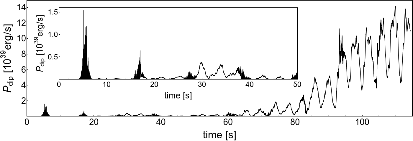
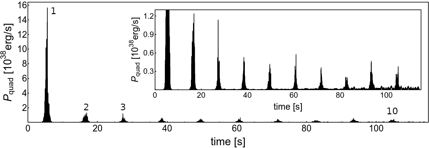
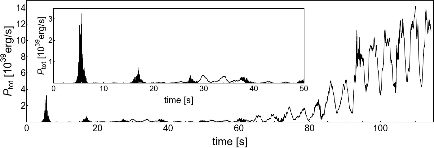
Figure 1: Electromagnetic radiation power of the system of a black hole and a white dwarf as a function of time. Successive frames (from top to bottom) show: electric dipole contribution, electric quadrupole part of radiation (with some passages through periastron marked by numbers, i.e. by $1$, $2$, $3$, and $10$), and sum of dipole and twice quadrupole contributions for the case when $M_{\rm BH}/m_{\rm wd}=10$.

Regular bursts are stronger exhibited for higher mass black hole-white dwarf binary systems, Fig. 2. This is because the dipole and quadrupole radiation power scales as $\mathcal{T}^{-6}$ and $\mathcal{T}^{-8}$, respectively (see Eqs. (LABEL:powerscaling) and (LABEL:scalingquad)). Increasing the mass of the black hole by a factor of $10^{2}$, the scaling parameter $\mathcal{T}$ decreases ten times resulting in much stronger (by two orders of magnitude) contribution from the quadrupole excitations than the dipole ones. Note that for the black hole with mass $M_{\rm BH}=10^{3}\,m_{\rm wd}$ its Schwarzschild radius equals about $0.4$ of the white dwarf radius, still much below the initial distance between the black hole and the white dwarf, which remains to be consistent with our numerical assumptions. Our simulations demonstrate that the quadrupole contribution to total emitted radiation becomes more important for the binaries with larger mass black holes.

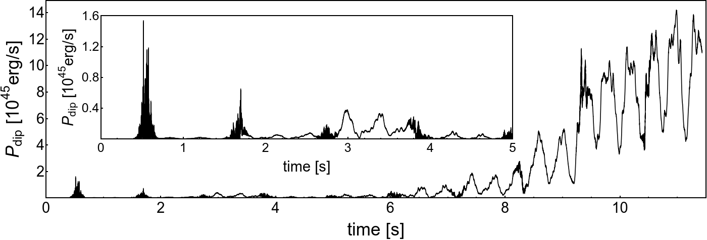
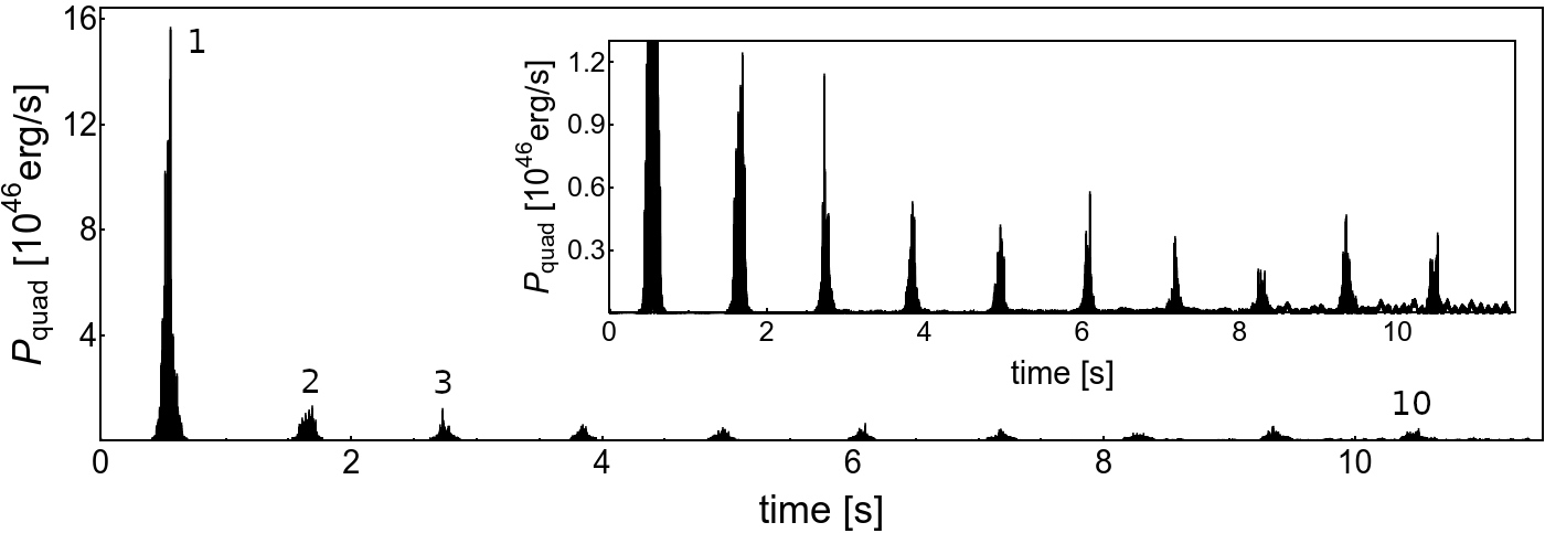
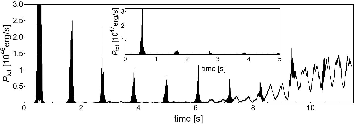
Figure 2: Electromagnetic radiation power of the system of a black hole and a white dwarf as a function of time. Successive frames (from top to bottom) show: electric dipole contribution, electric quadrupole part of radiation (with some passages through periastron marked by numbers, i.e. by $1$, $2$, $3$, and $10$), and sum of dipole and twice quadrupole contributions for the case when $M_{\rm BH}/m_{\rm wd}=10^{3}$.

Another interesting outcome of numerical simulations is that the accretion disk itself becomes a source of strong electric dipole radiation, see top frames in Figs. 1 and Figs. 2. Here, the accretion disc activates already after the third passage and becomes dominant at later time. Further properties of dipole radiation can be uncovered by looking at the dipole emission from a binary system in a particular direction. The power of radiation emitted in direction along angle $\Theta$ with respect to vector $\ddot{\bf{p}}$ is Griffiths

$$P\sim|\ddot{{\bf p}}|^{2}\,\sin^{2}{\Theta}\,.$$ (24)

Then the radiation power detected along $\hat{\bf{x}}$, $\hat{\bf{y}}$, and $\hat{\bf{z}}$ directions becomes $P_{x,y,z}\sim(\ddot{p})^{2}\,\Big{(}1-\ddot{p}_{x,y,z}^{2}/\ddot{p}^{2}\Big{)}$. Since $p_{z}=0$ one has $P_{z}\sim\ddot{p}^{\,2}$ and $P_{x}+P_{y}=P_{z}$. $P_{x,y,z}$ quantities are plotted in Fig. 3 for $M_{\rm BH}/m_{\rm wd}=10$. There is a qualitative difference in the observed dipole radiation depending on the observation angle. Since a charged mass dropped towards an accretion disc still (although for a limited time) orbits a black hole, it can be considered as a rotating electric dipole. Then it can be thought of as a superposition of two dipoles oscillating along $x$ and $y$ axes, respectively, and being out of phase by $\pi/2$. The energy emitted along $x$ and $y$ axes then exhibits a characteristic pattern as a function of time which is $\sim(1-\cos^{2}{\omega_{d}t})$ and $\sim(1-\sin^{2}{\omega_{d}t})$, respectively (see Fig. 3, blue and green curves). Here, $\omega_{d}$ is a frequency of rotating dipole (falling mass) which is higher than the frequency of orbiting white dwarf. Therefore, between two successive periastron passages one observes several oscillations in $P_{x}$ and $P_{y}$, whereas no such behaviour is visible in time-dependence of $P_{z}$. The properties of dipole-type radiation can tell us about the orientation of the orbital plane of a white dwarf with respect to the Earth. The accretion disc emits much weaker quadrupole-type radiation, see Figs. 1 and 2, middle frames. This remains true for both a stellar-mass and intermediate-mass black holes and is understandable since the structure of an accretion disc is mainly that of a rotating electric dipole type.

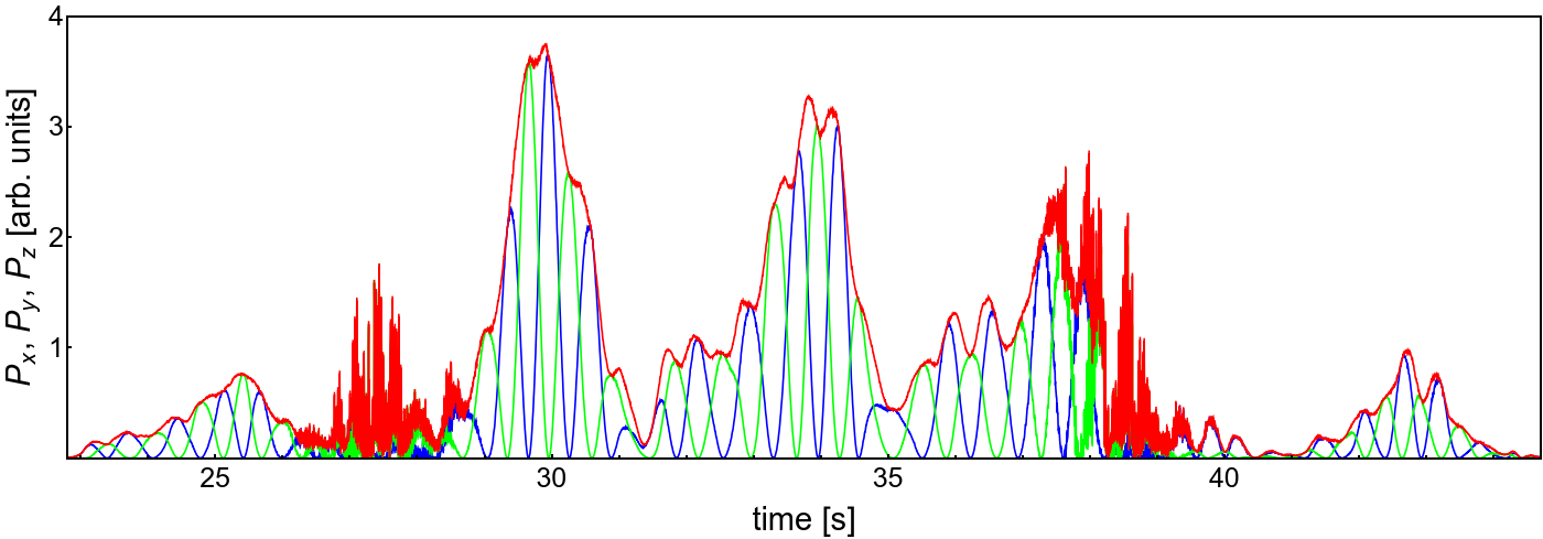
Figure 3: Power of electromagnetic radiation of the system of a black hole and a white dwarf emitted along $\hat{\bf{x}}$ (blue colour), $\hat{\bf{y}}$ (green colour), and $\hat{\bf{z}}$ (red colour) directions as a function of time, showing mainly the time period between the third and fourth periastron passages. Curve plotted in red colour is just the sum $P_{x}+P_{y}$.

Similar bursts of energy are visible while looking at the gravitational radiation power emitted by a binary black hole-white dwarf system, Fig. 4. However, the amount of energy radiated via gravitational waves remains a few orders of magnitudes lower than the energy emitted electromagnetically, compare Figs. 4 and 1 for the case of $M_{\rm BH}/m_{\rm wd}=10$. For such a stellar-mass black hole-white dwarf systems a peak gravitational-wave luminosity at a periastron passage is of the order of $10^{33}\,$erg s^-1 (Fig.4). For an intermediate-mass black holes ($M_{\rm BH}/m_{\rm wd}=10^{3}$) case a peak of radiation power increases up to $10^{39}\,$erg s^-1. This is, not surprisingly, much less than the maximum gravitational-wave luminosity detected in GW150914 event, the first observation of gravitational waves from the merger of two stellar-mass black holes Abbott16 , which was $10^{56}\,$erg s^-1. Two years later LIGO and Virgo detectors made the first observation of a binary neutron star inspiral, known as the signal GW170817 Abbott17 . The energy radiated via gravitational waves in this event was estimated from below as $0.025M_{\odot}c^{2}$. Combined with the knowledge of a duration of a gravitational wave signal, which lasted for approximately $100$ seconds, leads to average radiation power at least of the order of $10^{52}\,$erg s^-1. Merger of binary neutron stars was followed by a short $\gamma$-ray burst GRB 170817A Abbott17a located in the same sky position, thus linking a short bursts of $\gamma$ rays to coalescence of neutron stars. The power radiated electromagnetically by GRB 170817A event was estimated as of the order of $10^{46}\,$erg s^-1, much less than the power radiated via gravitational waves.

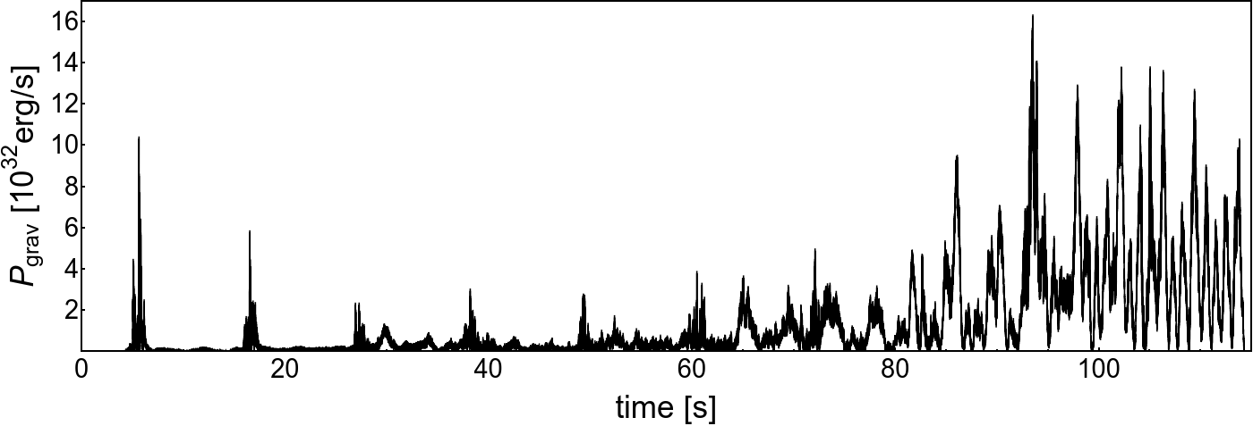
Figure 4: Gravitational radiation power of the system of a black hole and a white dwarf as a function of time for the case when $M_{\rm BH}/m_{\rm wd}=10$.

For the studied case of a binary system with a white dwarf moving along an eccentric orbit we observe tidal stripping of a white dwarf star and accompanying electromagnetic and gravitational radiation, with electromagnetic outcome being much stronger (compare Figs. 1 and 4). An important question is about frequencies at which binary system emits its gravitational energy. Here, we are particularly focused on the second periastron passage of a white dwarf, see Fig. 4. The gravitational energy emitted per frequency unit, i.e. power spectral density (PSD), is given by the following Fourier transform of gravitational radiation power, Eq. (LABEL:scalinggrav),

$${\rm PSD}_{grav}=\left|{\cal{F}}\left[\sqrt{\,{\rm P}_{grav}}\right]\right|^{2}$$ (25)

and is depicted in Fig. 5. Clearly, the energy is mainly radiated at low frequencies, below $\omega/2\pi\approx 1\,$Hz, see Inset (more than $95$ % of the whole energy is emitted within the range of frequencies $\omega/2\pi<10\,$Hz). Already planned gravitational-wave observatory in space, the Laser Interferometer Space Antenna (LISA), is supposed to work in frequency range covering the one visible in inset in Fig. 5.

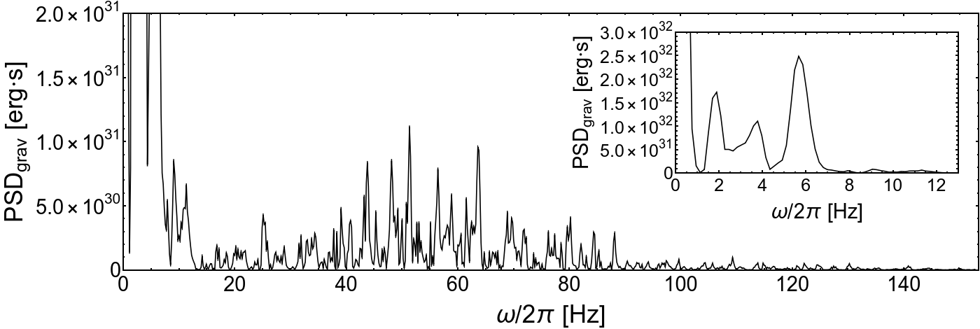
Figure 5: Power spectral density of gravitational waves emitted during the second periastron passage (see Fig. 4) for the case when $M_{\rm BH}/m_{\rm wd}=10$. Inset shows PSD for low frequencies, below $\omega/2\pi=10\,$Hz.

VI Conclusions

In summary, we have studied the electromagnetic and gravitational radiation coming out of the system of a white dwarf orbiting a black hole. As a model of a white dwarf star we consider a zero temperature Bose-Fermi droplet of attractively interacting degenerate atomic bosons and spin-polarized atomic fermions. Our quantum hydrodynamics based simulations indeed show that the black hole-white dwarf binary system emits the electromagnetic energy in bursts, while crossing the periastron area. Such regular high energy blasts resemble ultraluminous X-ray bursts uncovered recently Irwin16 . Our simulations show that binary systems with heavier black holes radiate mostly in a quadrupole mode. On the other hand, the accretion disc emits energy mainly via dipole-type radiation, provided stellar- and intermediate-mass black holes are considered. This property can be used to determine the orientation of an orbital plane of a black hole-white dwarf binary system with respect to the observer on the Earth. Our simulations also show that at periastron the gravitational energy is emitted mainly at the very low frequencies. Moreover, they demonstrate that the binary system becomes a source of continues gravitational radiation as soon as the accretion disc is formed.

Appendix A Energy contributions

The intrinsic kinetic energy of an ideal Fermi gas is

$$T=\int d{\bf r}\,\left(\kappa_{k}\,n_{F}^{5/3}-\xi\,\frac{\hbar^{2}}{8m_{F}}\frac{(\nabla n_{F})^{2}}{n_{F}}\right)$$ (26)

with $\kappa_{k}=(3/10)\,(6\pi^{2})^{2/3}\,\hbar^{2}/m_{F}$ and $\xi=1/9$ Weizsacker ; Kirznits ; Oliver .

The boson-fermion interaction energy is

$$E_{BF} = \int d{\bf r}\,g_{BF}\,n_{B}({\bf r})n_{F}({\bf r})$$ (27)

$$+ C_{BF}\int d{\bf r}\,n_{B}\,n_{F}^{4/3}A(w,\alpha)\,,$$

where $w=m_{B}/m_{F}$ and $\alpha=2w(g_{B}n_{B}/\varepsilon_{F})$ are dimensionless parameters, $C_{BF}=(6\pi^{2})^{2/3}\hbar^{2}a_{BF}^{2}/2m_{F}$, and the function $A(w,\alpha)$ is given in a form of integral Giorgini02

$$A(w,\alpha)=\frac{2(1+w)}{3w}\left(\frac{6}{\pi}\right)^{2/3}\int^{\infty}_{0}{\rm d}k\int^{+1}_{-1}{\rm d}{\Omega}$$

$$\left[1-\frac{3k^{2}(1+w)}{\sqrt{k^{2}+\alpha}}\int^{1}_{0}{\rm d}qq^{2}\frac{1-\Theta(1-\sqrt{q^{2}+k^{2}+2kq\Omega})}{\sqrt{k^{2}+\alpha}+wk+2qw\Omega}\right],$$

(28)

with $\Theta()$ being the step theta-function.

The bosonic quantum pressure term is

$$V_{q}=-\hbar^{2}/(2m_{B})\,(\nabla^{2}\sqrt{n_{B}})/\sqrt{n_{B}}\,.$$ (29)

The interaction between bosons, including the famous Lee-Huang-Yang correction LHY57 , is

$$E_{B}=g_{B}n_{B}^{2}/2+C_{LHY}\int d{\bf r}\,n_{B}^{5/2}$$ (30)

with $C_{LHY}=64/(15\sqrt{\pi})\,g_{B}\,a_{B}^{3/2}$. $g_{B}$ and $g_{BF}$ appearing in the above energy expressions are coupling constants for contact interactions between atoms PitaevskiiStringari , with $g_{B}=4\pi\hbar^{2}a_{B}/m_{B}$ and $g_{BF}=2\pi\hbar^{2}a_{BF}/\mu$, where $a_{B}$ ($a_{BF}$) is the scattering length corresponding to the boson-boson (boson-fermion) interaction and $\mu=m_{B}\,m_{F}/(m_{B}+m_{F})$ is the reduced mass.

References

- (1) A. V. Tutukov, A. V. Fedorova, Astronomy Reports, 51, 291 (2007).
- (2) J.A. Irwin, W.P. Maksym, G.R. Sivakoff, A.J. Romanowsky, D. Lin, T. Speegle, I. Prado, D. Mildebrath, J. Strader, J. Liu, and J.M. Miller, Nature 538, 356 (2016).
- (3) G.R. Sivakoff, C.L. Sarazin, and A. Jordán, Astrophys. J. 624, L17 (2005).
- (4) A. Tiengo, P. Esposito, M. Toscani, G. Lodato, M. Arca Sedda, S.E. Motta, F. Contato, M. Marelli, R. Salvaterra, A. De Luca, A&A 661, A68 (2022).
- (5) T. J. Maccarone, MNRAS 364, 971 (2005).
- (6) R.-F. Shen, Astrophys. J. Lett. 871, L17 (2019).
- (7) J.H. Krolik, T. Piran, ApJ, 743, 134 (2011).
- (8) T. Karpiuk, M. Nikołajuk, M. Gajda, and M. Brewczyk, Sci. Rep. 11, 2286 (2021).
- (9) G. Miniutti et al., Nature 573, 381 (2019).
- (10) R. Arcodia et al., Nature 592, 704 (2021).
- (11) Zhu Liu, A. Malyali, M. Krumpe, et al., preprint arXiv: 2208.12452
- (12) D. Rakshit, T. Karpiuk, M. Brewczyk, and M. Gajda, SciPost Phys. 6, 079 (2019).
- (13) D. Rakshit, T. Karpiuk, P. Zin, M. Brewczyk, M. Lewenstein, and M. Gajda, New J. Phys. 21, 073027 (2019).
- (14) T. Karpiuk, M. Gajda, and M. Brewczyk, New J. Phys. 22, 103025 (2020).
- (15) R.P. Feynman, Int. J. Theor. Phys. 21, 467 (1982).
- (16) R.P. Feynman, Found. Phys. 16 507 (1986).
- (17) M. Greiner, O. Mandel, T. Esslinger, T.W. Hänsch, and I. Bloch, Nature 415, 40 (2002).
- (18) C.-L. Hung, X. Zhang, N. Gemelke, and C. Chin, Nature 470, 236 (2011).
- (19) C.-L. Hung, V. Gurarie, and C. Chin, Science 341, 1213 (2013).
- (20) J.R.M. de Nova, K. Golubkov, V.I. Kolobov, and J. Steinhauer, Nature 569, 688 (2019).
- (21) R. Goldsbury, J. Heyl, H.B.Richer, P. Bergeron, A. Dotter, J.S. Kalirai, J. MacDonald, R.M. Rich, P.B. Stetson, P.-E. Tremblay, and K.A. Woodley, ApJ 760, 78 (2012).
- (22) G. Fontaine, P. Brassard, and P. Bergeron, PASP 113, 409 (2001).
- (23) D.L. Kaplan, J. Boyles, B.H. Dunlap, S.P. Tendulkar, A.T. Deller, S.M. Ransom, M.A. McLaughlin, D.R. Lorimer, I.H. Stairs, ApJ 789, 119 (2014).
- (24) M.E. Tannock et al. AJ 161, 224 (2021).
- (25) L. Mestel, MNRAS 112, 583 (1952)
- (26) M. Brewczyk, M. Gajda, and K. Rza̧żewski, J. Phys. B 40, R1 (2007).
- (27) G. Gabadadze, R.A. Rosen, Phys. Lett. B 658, 266 (2008).
- (28) G. Gabadadze, R.A. Rosen, JCAP 2008, 030 (2008).
- (29) G. Gabadadze, D. Pirtskhalava, JCAP 2009, 017 (2009).
- (30) M.E. Mosquera, O. Civitarese, O.G. Benvenuto, and M.A. De Vito, Phys. Lett. B 683, 119 (2010).
- (31) H.R. Hertz, Annalen der Physik 267, 421 (1887).
- (32) J.C. Maxwell, A Treatise on Electricity and Magnetism (Dover, New York, 1954).
- (33) D.J. Griffiths, Introduction to electrodynamics (New Jersey, Prentice Hall, 1999).
- (34) J.D. Jackson, Classical electrodynamics (New York, Wiley, 1999).
- (35) B.P. Abbott et al., Phys. Rev. Lett. 116, 061102 (2016).
- (36) M. Maggiore, Gravitational waves (Oxford University Press, New York, 2008).
- (37) P. Jaranowski and A. Królak, Analysis of Gravitational-Wave Data (Cambridge University Press, Cambridge, 2009).
- (38) R.A. Hulse and J.H. Taylor, Astrophys. J. 191, L59 (1974).
- (39) R.A. Hulse and J.H. Taylor, Astrophys. J. 195, L51 (1975).
- (40) J.H. Taylor, L.A. Fowler, and J.M. Weisberg, Nature 277, 437 (1979).
- (41) E. Madelung, Z. Phys. 40, 322 (1927).
- (42) H. Frölich, Physica 37, 215 (1967).
- (43) C.Y. Wong and J.A. McDonald, Phys. Rev. C 16, 1196 (1977).
- (44) N.H. March and B.M. Deb, The single-particle density in physics and chemistry (Academic Press, London, 1987).
- (45) J.A. Ball, J.A. Wheeler, and E.L. Fireman, Rev. Mod. Phys. 45, 333 (1973).
- (46) C.F. Weizsäcker, Z. Phys. 96, 431 (1935).
- (47) D.A. Kirznits, Sov. Phys. JETP 5, 64 (1957).
- (48) G.L. Oliver and J.P. Perdew, Phys. Rev. A 20, 397 (1979).
- (49) T.D. Lee, K. Huang, and C.N. Yang, Phys. Rev. 106, 1135 (1957).
- (50) B.Kr. Dey and B.M. Deb, Int. J. Quantum Chem. 70, 441 (1998).
- (51) A. Domps, P.-G. Reinhard, and E. Suraud, Phys. Rev. Lett. 80, 5520 (1998).
- (52) P.T. Grochowski, T. Karpiuk, M. Brewczyk, and K. Rzążewski, Phys. Rev. Lett. 119, 215303 (2017).
- (53) P.T. Grochowski, T. Karpiuk, M. Brewczyk, and K. Rzążewski, Phys. Rev. Lett. 125, 103401 (2020).
- (54) B. Paczyńsky and P.J. Wiita, A&A 88, 23 (1980).
- (55) K. Gawryluk, T. Karpiuk, M. Gajda, K. Rzążewski, and M. Brewczyk, Int. J. Comput. Math. 95, 2143 (2018).
- (56) B.J. DeSalvo, K. Patel, J. Johansen, and C. Chin, Phys. Rev. Lett. 119, 233401 (2017).
- (57) B.J. DeSalvo, K. Patel, G. Cai, and C. Chin, Nature 568, 61 (2019).
- (58) R. Pires, J. Ulmanis, S. Häfner, M. Repp, A. Arias, E.D. Kuhnle, and M. Weidemüller, Phys. Rev. Lett. 112, 250404 (2014).
- (59) B.P. Abbott et al., Phys. Rev. Lett. 119, 161101 (2017).
- (60) B.P. Abbott et al., Astrophys. J. Lett. 848, L13 (2017).
- (61) L. Viverit and S. Giorgini, Phys. Rev. A 66, 063604 (2002).
- (62) L. Pitaevskii and S. Stringari, Bose-Einstein Condensation (Oxford University Press, Oxford, 2003).