Explosion of a Minimum-Mass Neutron Star within Relativistic Hydrodynamics

National Research Center ‘‘Kurchatov Institute’’, Moscow, 123182 Russia¹

The relativistic hydrodynamics equations are adapted for the spherically symmetric case and the Lagrangian form. They are used to model the explosive disruption of a minimum-mass neutron star, a key ingredient of the stripping model for short gamma-ray bursts. The shock breakout from the neutron star surface accompanied by the acceleration of matter to ultrarelativistic velocities is studied. A comparison with the results of previously published nonrelativistic calculations is made.

Keywords: neutron stars, relativistic hydrodynamics, shock waves, gamma-ray bursts.

 
^∗ email: $<$yudin@itep.ru$>$

INTRODUCTION

On August 17, 2017, the event GW170817 with parameters corresponding to merging neutron stars occurred on the LIGO and Virgo gravitational-wave antennas (Abbott et al. 2017). In addition, the FERMI and INTEGRAL satellites detected the accompanying gamma-ray burst GRB170817A almost simultaneously. Thus, the connection between the merging of neutron stars (NSs) and short gammaray bursts (GRBs) (Blinnikov et al. 1984) was directly confirmed for the first time.

However, this GRB turned out to be peculiar, which renewed the nearly faded interest in the stripping model for short GRBs (Blinnikov et al. 2021). In contrast to the universally accepted NS merging model, in the stripping model two NSs, having come closer together due to the energy losses through gravitational-wave radiation, do not merge, but begin to exchange mass, with the more massive one swallows (strips) its less massive companion (Clark and Eardley 1977). The latter, having reached a configuration corresponding to the minimum mass of stable NSs ($\sim 0.1M_{\odot}$), explodes to produce a GRB.

The details of the explosion of a minimum-mass NS (MMNS) were first calculated by Blinnikov et al. (1990) (see also Sumiyoshi et al. 1998). An important fact for us here is that the matter expansion velocities after the explosion are, on average, $\sim$10% of the speed of light. In addition, the shock from the explosion, when breaking out, is accelerated as it propagates along a descending density profile. A computation of this process within nonrelativistic hydrodynamics with a good resolution can lead and actually leads, as we will show, to velocities exceeding the speed of light. Therefore, studying this process in terms of relativistic hydrodynamics is topical. In this case, the gravitational field may be deemed relatively weak: the MMNS has a factor of 10 lower mass and a factor of 10 larger radius than does an ordinary NS; consequently, the general relativity (GR) effects for it are a factor of 100 smaller than those for an ordinary NS. It seems to us that the most appropriate approach to study this problem is the approximation proposed in Hwang and Noh (2016), which we will use.

BASIC EQUATIONS

Let us write the relativistic hydrodynamics equations following Hwang and Noh (2016). The gravitational field is assumed to be weak (i.e., the GR effects are small), but the matter velocities and the energy density in comparison with the rest mass are not assumed to be small. We will write the original equations from Hwang and Noh (2016) and then will transform them to a form meeting our goals or, more specifically, to a form suggesting the spherical symmetry of the problem and the Lagrangian form. Quantities like the time $t$, the radial coordinate $r$, and the matter velocity $v$ are defined in the laboratory frame, while quantities like the density $\rho_{\mathrm{b}}$, the pressure $P$, etc. are defined in the comoving frame.

Continuity Equation

The original continuity equation is:

$$\frac{d\rho_{\mathrm{b}}}{dt}+\rho_{\mathrm{b}}\Big{(}\mathrm{div}\,\vec{v}+\frac{d\ln\gamma}{dt}\Big{)}=0.$$ (1)

Here $\rho_{\mathrm{b}}$ is the baryonic density of the matter, $\vec{v}$ is its velocity, and $\gamma$ is the Lorentz factor:

$$\gamma\equiv\frac{1}{\sqrt{1{-}v^{2}/c^{2}}},$$ (2)

where $c$ is the speed of light. The total time derivative is:

$$\frac{d}{dt}=\frac{\partial}{\partial t}+(\vec{v}\cdot\vec{\nabla}).$$ (3)

We will rewrite Eq. (1) as:

$$\frac{d\ln(\rho_{\mathrm{b}}\gamma)}{dt}+\frac{1}{r^{2}}\frac{\partial\left(r^{2}v\right)}{\partial r}=0,$$ (4)

where $r$ is the radius (Eulerian coordinate) and the divergence is written for the case of spherical symmetry. Let us now introduce a natural definition for the Lagrangian (mass) coordinate $m_{\mathrm{b}}$ (baryonic mass):

$$\frac{\partial m_{\mathrm{b}}}{\partial r}=4\pi r^{2}\rho_{\mathrm{b}}\gamma,$$ (5)

where, in comparison with the nonrelativistic case, the additional factor $\gamma$ appears on the right-hand side. Let us write this expression as

$$\frac{1}{\rho_{\mathrm{b}}\gamma}=\frac{4\pi}{3}\frac{\partial r^{3}}{\partial m_{\mathrm{b}}}.$$ (6)

Let us show that this is another form of the continuity equation (4). For this purpose, let us differentiate it with respect to time:

$$-\frac{1}{(\rho_{\mathrm{b}}\gamma)^{2}}\frac{d(\rho_{\mathrm{b}}\gamma)}{dt}=4\pi\frac{\partial(r^{2}v)}{\partial m_{\mathrm{b}}},$$ (7)

where we used the fact that $v\equiv dr/dt$. Substituting here $\partial m_{\mathrm{b}}/\partial r$ from (5), we will obtain exactly (4). We will use (6) as the main Lagrangian form of the continuity equation and $m_{\mathrm{b}}$ as the Lagrangian coordinate.

Energy Equation

The energy equation in Hwang and Noh (2016) is written as

$$\frac{d\rho}{dt}+\left(\rho+P/c^{2}\right)\Big{(}\mathrm{div}\,\vec{v}+\frac{d\ln\gamma}{dt}\Big{)}=R_{\mathrm{E}},$$ (8)

where $P$ is the matter pressure, $\rho=\rho_{\mathrm{b}}(1+E/c^{2})$ is the total mass–energy density, and $E$ is the internal energy of the matter per unit mass. The expression for the right-hand side $R_{\mathrm{E}}$ is written via the spatial part $\Pi_{ij}$ of the anisotropic energy–momentum tensor $\pi_{\alpha\beta}$, which is related to the total energy–momentum tensor of the matter $T_{\alpha\beta}$ by the relation

$$T_{\alpha\beta}=(\rho c^{2}+P)u_{\alpha}u_{\beta}+Pg_{\alpha\beta}+\pi_{\alpha\beta},$$ (9)

where $u_{\alpha}$ is the 4-velocity and $g_{\alpha\beta}$ is a metric tensor with signature $(-,+,+,+)$. In what follows, we adopt the condition that the Greek and Latin indices run the values of $(0{\div}3)$ and $(1{\div}3)$, respectively. We will write out the specific form of $R_{\mathrm{E}}$ below.

Subtracting the continuity equation (1) from (8), after simple transformations it is easy to obtain the energy equation in the form

$$\frac{dE}{dt}+P\frac{d}{dt}\!\left(\!\frac{1}{\rho_{\mathrm{b}}}\!\right)=\frac{R_{\mathrm{E}}c^{2}}{\rho_{\mathrm{b}}}.$$ (10)

Equation of Motion

The equation of motion is

$$\frac{d\vec{v}}{dt}=\vec{a}_{\mathrm{G}}-\frac{\vec{\nabla}P+\vec{v}\dot{P}/c^{2}+\vec{R}_{\mathrm{V}}}{\gamma^{2}(\rho+P/c^{2})},$$ (11)

where $\vec{a}_{\mathrm{G}}=-\vec{\nabla}\varphi$ is the gravitational acceleration and $\varphi$ is the gravitational potential the equation for which is given below. The dot in $\dot{P}$ denotes a partial time derivative and $\vec{R}_{\mathrm{V}}$ is the part of the acceleration that depends on $\Pi_{ik}$, whose explicit form will be discussed later.

ARTIFICIAL VISCOSITY

To write the complete system of relativistic hydrodynamics equations in the final form, it remains to determine the specific form of the tensor $\Pi_{ij}$. Here we will consider the contribution to it only from the artificial viscosity needed to calculate the shock waves. We will follow the paper by Liebendoerfer et al. (2001), where the following general relativistic expression for the viscosity tensor $Q_{\alpha\beta}$ was proposed:

$$Q_{\alpha\beta}=\triangle l^{2}\rho_{\mathrm{b}}u^{\mu}_{;\mu}\Big{[}\varepsilon_{\alpha\beta}-\frac{1}{3}u^{\mu}_{;\mu}P_{\alpha\beta}\Big{]},$$ (12)

which is valid at $u^{\mu}_{;\mu}<0$, otherwise it is zero. Here, $\triangle l$ is the characteristic shock front ‘‘smearing’’ width, $P_{\alpha\beta}=u_{\alpha}u_{\beta}+g_{\alpha\beta}$, and

$$\varepsilon_{\alpha\beta}=\frac{1}{2}\left(u_{\alpha;\mu}P^{\mu}_{\beta}+u_{\beta;\mu}P^{\mu}_{\alpha}\right).$$ (13)

Using the continuity equation (1), the derivative $u^{\mu}_{;\mu}$ can be represented as

$$u^{\mu}_{;\mu}=\frac{1}{c}\frac{\partial\gamma}{\partial t}+\frac{\partial}{\partial x_{i}}\!\left(\frac{\gamma v_{i}}{c}\right)=-\frac{\gamma}{c}\frac{d\ln\rho_{\mathrm{b}}}{dt}.$$ (14)

Hence it can be seen that the artificial viscosity (12) does ‘‘work’’ only during matter compression. To calculate the remaining quantities, we will use the spherical symmetry of the problem. We will write the velocity as $\vec{v}=v\vec{r}/r$ and express the 4-velocity via $\gamma$ as $u^{\alpha}=(\gamma,\frac{\vec{r}}{r}\sqrt{\gamma^{2}{-}1})$. We will also use the definition (3) and, as a consequence, the fact that for any scalar $a$

$$u^{\mu}a_{;\mu}=\frac{\gamma}{c}\frac{da}{dt}.$$ (15)

In addition, we will use the relationship between the total time derivatives of $\rho_{\mathrm{b}}$ and $\gamma$ and the partial derivative $\partial v/\partial r$ following from (4). The final expression will be written as (recall that for the tensor $\Pi_{ij}$ we need only the spatial components)

$$Q_{ij}=\triangle l^{2}\rho_{\mathrm{b}}\frac{\gamma^{2}}{3}\frac{d\ln\rho_{\mathrm{b}}}{dt}\Big{(}\frac{d\ln\rho_{\mathrm{b}}}{dt}+\frac{3v}{r}\Big{)}\Big{[}(2\gamma^{2}{+}1)\frac{r_{i}r_{j}}{r^{2}}-\delta_{ij}\Big{]}.$$ (16)

Since we work in Lagrangian variables, it is convenient to replace the length scale $\triangle l$ via the characteristic baryonic mass $\triangle m_{\mathrm{b}}$ using (5). Finally, we will write

$$\Pi_{ij}=Q_{ij}=\frac{Q}{2}\left[(2\gamma^{2}{+}1)\frac{r_{i}r_{j}}{r^{2}}-\delta_{ij}\right],$$ (17)

where the factor $1/2$ is introduced for convenience and $Q$ is the ordinary artificial viscosity, which after some transformations takes the form

$$Q=-\frac{2}{3}\left(\!\frac{\triangle m_{\mathrm{b}}}{4\pi r^{2}}\!\right)^{2}\frac{d}{dt}\!\left(\!\frac{1}{\rho_{\mathrm{b}}}\!\right)\frac{d}{dt}\Big{(}\!\ln(\rho_{\mathrm{b}}r^{3})\!\Big{)},$$ (18)

for $Q>0$, otherwise $Q=0$. This expression has the following peculiarity noted in Liebendoerfer et al. (2001): it becomes zero non only during matter expansion (the first factor with $d/dt$), but also during homologous compression (i.e., for $v\propto r$, the second factor), which allows the nonphysical matter overheating to be avoided.

POISSON EQUATION

The generalization of the Poisson equation for the gravitational potential is written as (Hwang and Noh 2016):

$$\triangle\varphi=4\pi G\Big{(}\rho+3P/c^{2}+\frac{2}{c^{2}}\big{[}\gamma^{2}v^{2}(\rho+P/c^{2})+\Pi^{i}_{i}\big{]}\Big{)}.$$ (19)

Using the explicit form (17) of the tensor $\Pi_{ij}$, we can find its convolution: $\Pi^{i}_{i}=(\gamma^{2}{-}1)Q$. The equation for the gravitational acceleration $a_{\mathrm{G}}=-\partial\varphi/\partial r$ is then written as

$$\gamma\frac{\partial\left(r^{2}a_{\mathrm{G}}\right)}{\partial m_{\mathrm{b}}}={-}G\Big{(}2\gamma^{2}{-}1+\frac{(2\gamma^{2}{-}1)E}{c^{2}}+\frac{(2\gamma^{2}{+}1)P}{\rho_{\mathrm{b}}c^{2}}+\frac{2(\gamma^{2}{-}1)Q}{\rho_{\mathrm{b}}c^{2}}\Big{)},$$ (20)

where we took into account the spherical symmetry of the problem.

RIGHT-HAND SIDE OF THE ENERGY EQUATION

The expression for the right-hand side of the energy equation $R_{\mathrm{E}}$ is

$$R_{\mathrm{E}}=-\frac{1}{c^{2}}\Big{[}\Pi^{j}_{i}\nabla_{j}v^{i}+\Pi_{ij}\frac{v^{i}\dot{v}^{j}}{c^{2}}\Big{]},$$ (21)

where the dot again denotes a partial time derivative. Writing the velocity as $\vec{v}=v\vec{r}/r$ and using Eq. (17) for the tensor $\Pi_{ij}$ , it is easy to obtain

$$R_{\mathrm{E}}=\frac{Q}{c^{2}}\Big{[}\frac{v}{r}-\gamma^{2}\Big{(}\frac{\partial v}{\partial r}+\frac{v\dot{v}}{c^{2}}\Big{)}\Big{]}.$$ (22)

The expression in square brackets is transformed using the continuity equation (4) into

$$\frac{d\ln\rho_{\mathrm{b}}}{dt}+\frac{3v}{r}=\frac{d}{dt}\Big{(}\!\ln(\rho_{\mathrm{b}}r^{3})\!\Big{)}.$$ (23)

The energy balance equation (10) will then finally be written as

$$\frac{dE}{dt}+P\frac{d}{dt}\!\left(\!\frac{1}{\rho_{\mathrm{b}}}\!\right)=\frac{Q}{\rho_{\mathrm{b}}}\frac{d}{dt}\Big{(}\!\ln(\rho_{\mathrm{b}}r^{3})\!\Big{)}.$$ (24)

Remarkably, the same factor with the total time derivative of $\rho_{\mathrm{b}}r^{3}$ as that in the definition of the artificial viscosity (18) appeared on the right-hand side of (24).

RIGHT-HAND SIDE OF THE EQUATION OF MOTION

The quantity $\vec{R}_{\mathrm{V}}$ on the right-hand side of the equation of motion (11) looks as follows:

$$(R_{\mathrm{V}})_{i}=\Pi^{j}_{i,j}-\frac{1}{c^{2}}\left[v_{i}(\Pi^{k}_{j}v^{j})_{,k}-(\Pi_{ij}v^{j})^{\cdot}\right]-\frac{v_{i}}{c^{4}}(\Pi_{jk}v^{j}v^{k})^{\cdot}.$$ (25)

Given the spherical symmetry of the problem and the explicit form (17) for the tensor $\Pi_{ij}$, we will obtain a number of relations:

$$\Pi_{ij}v^{j} =\frac{r_{i}}{r}v\gamma^{2}Q,$$ (26)

$$\Pi_{ij}v^{j}v^{j} =v^{2}\gamma^{2}Q=(\gamma^{2}{-}1)Qc^{2}.$$ (27)

The first term in (25) is

$$\Pi_{i,j}^{j}=\frac{r_{i}}{r}\Big{[}\gamma^{2}\frac{\partial Q}{\partial r}+\Big{(}\frac{2\gamma^{2}{+}1}{r}+\frac{\partial\gamma^{2}}{\partial r}\Big{)}Q\Big{]}.$$ (28)

The factor at $v_{i}$ in the first term in square brackets (25) is

$$(\Pi^{k}_{j}v^{j})_{,k}=\frac{1}{r^{2}}\frac{\partial}{\partial r}\big{(}v\gamma^{2}r^{2}Q\big{)}.$$ (29)

Collecting all terms, we finally can write

$$(R_{\mathrm{V}})_{i}=\frac{r_{i}}{r}\left[\frac{\partial Q}{\partial r}+\frac{3Q}{r}+\gamma^{2}\frac{dv}{dt}\frac{Q}{c^{2}}+\frac{v}{c^{2}}\frac{\partial Q}{\partial t}\right].$$ (30)

Substituting this expression into (11), after some transformations using, in particular, the energy equation (24), we will obtain the equation of motion

$$\frac{d}{dt}\Big{(}\gamma v\big{[}1+\frac{E{+}(P{+}Q)/\rho_{\mathrm{b}}}{c^{2}}\big{]}\Big{)}=\gamma^{3}\Big{(}1+\frac{E{+}P/\rho_{\mathrm{b}}}{c^{2}}\Big{)}a_{\mathrm{G}}-4\pi r^{2}\frac{\partial(P{+}Q)}{\partial m_{\mathrm{b}}}-\frac{3Q}{\gamma r\rho_{\mathrm{b}}}.$$ (31)

DIMENSIONLESS FORM OF THE EQUATIONS

For numerical calculations of hydrodynamic processes in a star it is convenient to have the above equations in a dimensionless form. We will use the system of units based on the total mass $M_{\mathrm{s}}$ and initial radius $R_{\mathrm{s}}$of the star. The units of time, velocity, density, energy per unit mass, and pressure are

$$[t] =\sqrt{\frac{R_{\mathrm{s}}^{3}}{GM_{\mathrm{s}}}},$$ (32)

$$[v] =\sqrt{\frac{GM_{\mathrm{s}}}{R_{\mathrm{s}}}},$$ (33)

$$[\rho] =\frac{M_{\mathrm{s}}}{4\pi R_{\mathrm{s}}^{3}},$$ (34)

$$[E] =\frac{GM_{\mathrm{s}}}{R_{\mathrm{s}}},$$ (35)

$$[P] =\frac{GM_{\mathrm{s}}^{2}}{4\pi R_{\mathrm{s}}^{4}}.$$ (36)

It is also convenient to introduce the relativistic parameter $r_{\mathrm{g}}$:

$$r_{\mathrm{g}}=\frac{GM_{\mathrm{s}}}{R_{\mathrm{s}}c^{2}}.$$ (37)

The parameter $\gamma$ is then

$$\gamma=\frac{1}{\sqrt{1-r_{\mathrm{g}}\hat{v}^{2}}},$$ (38)

where $\hat{v}$ is the dimensionless velocity. The continuity equation (6) in dimensionless variables takes the form

$$\frac{3}{\hat{\rho}_{\mathrm{b}}\gamma}=\frac{\partial\hat{r}^{3}}{\partial m},$$ (39)

where $\hat{\rho}_{\mathrm{b}}$, $\hat{r}$, and $m$ are the dimensionless density, radius, and mass coordinate, respectively.

For a further analysis it will be convenient to introduce the following dimensionless quantities: $\epsilon$ for the internal energy $E$, $p$ for the ratio $P/\rho_{\mathrm{b}}$, and $q$ for $Q/\rho_{\mathrm{b}}$. The expression for the artificial viscosity (18) will then be written as

$$q=-\frac{(\triangle m)^{2}}{3\hat{r}^{4}}\frac{d}{d\tau}\!\left(\!\frac{1}{\hat{\rho}_{\mathrm{b}}^{2}}\!\right)\frac{d}{d\tau}\Big{(}\!\ln(\hat{\rho}_{\mathrm{b}}\hat{r}^{3})\!\Big{)},$$ (40)

where $\tau$ is the dimensionless time.

The energy equation (24) will take the form

$$\frac{d\epsilon}{d\tau}-p\frac{d\ln\hat{\rho}_{\mathrm{b}}}{d\tau}=q\frac{d}{d\tau}\Big{(}\!\ln(\hat{\rho}_{\mathrm{b}}\hat{r}^{3})\!\Big{)}.$$ (41)

Equation (20) for the gravitational acceleration will be written as

$$-\gamma\frac{\partial\left(\hat{r}^{2}\hat{a}_{\mathrm{G}}\right)}{\partial m}=2\gamma^{2}{-}1+r_{\mathrm{g}}\big{[}(2\gamma^{2}{-}1)\epsilon+(2\gamma^{2}{+}1)p+2(\gamma^{2}{-}1)q\big{]}.$$ (42)

And, finally, the equation of motion (31) will take the form

$$\frac{d}{d\tau}\big{(}\gamma\hat{v}\big{[}1+r_{\mathrm{g}}(\epsilon+p+q)\big{]}\big{)}=\gamma^{3}\big{(}1+r_{\mathrm{g}}(\epsilon+p)\big{)}\hat{a}_{\mathrm{G}}-\hat{r}^{2}\frac{\partial\big{(}(p+q)\hat{\rho}_{\mathrm{b}}\big{)}}{\partial m}-\frac{3q}{\gamma\hat{r}}.$$ (43)

Equations (39), (41), and (43) in combination with the definitions (38), (40), and (42) (and the equality $\hat{v}=d\hat{r}/d\tau$) comprise the complete system of ideal relativistic hydrodynamics equations.

FORMULATION OF THE EXPLOSION PROBLEM

In the formulation of the initial conditions in the problem of the explosion of a minimum-mass neutron star (MMNS) we will largely follow the paper of Blinnikov et al. (1990).

For the equation of state (EoS) of the matter we use a universally accepted, though significantly simplified, approach: thermodynamic quantities, such as the pressure and the internal energy, are represented by sums:

$$P=P_{0}(\rho_{\mathrm{b}})+\frac{\rho_{\mathrm{b}}kT}{m_{\mathrm{u}}}+\frac{aT^{4}}{3},$$ (44)

$$E=E_{0}(\rho_{\mathrm{b}})+\frac{3kT}{2m_{\mathrm{u}}}+\frac{aT^{4}}{\rho_{\mathrm{b}}},$$ (45)

where $T$ is the temperature, $k$ is the Boltzmann constant, $m_{\mathrm{u}}$ is the atomic mass unit, and $a=8\pi^{5}k^{4}/15(hc)^{3}$ is the radiation density constant. The second and third terms in (44–45) represent the contribution of the ideal gas and the radiation, respectively. For the terms $P_{0}$ and $E_{0}$ we use the fits proposed by Haensel and Potekhin (2004). They describe the properties of NS matter at temperature $T=0$ in a wide density range. For our calculations we chose the BSk22 fit. Naturally, Eqs. (44–45) describe very roughly the temperature part of the matter thermodynamics and may be considered only as the first approximation to reality.

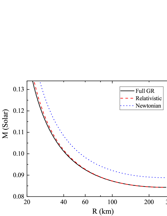
Figure 1: NS mass–radius diagram near the minimum mass. The blue dotted and black solid lines indicate the nonrelativistic case and the solution of the GR equations, respectively. The red dashed line indicates our approach.

Now it is necessary to determine the MMNS parameters: for this purpose, we construct a sequence of NS models parameterized by a decreasing central density (see, e.g., Haensel et al. 2007) and find the MMNS in the sequence. The NS matter temperature is assumed to be zero. Figure 1 shows the lower part of the NS mass–radius diagram computed within several approaches. The blue dotted line indicates the nonrelativistic case. The black solid line indicates the solution of the Tolman–Oppenheimer–Volkoff equations (see, e.g., Weinberg 1972). The red dashed line indicates our approach. As the central density decreases, the mass of the star drops, while its radius increases. Each curve in the figure ends with the MMNS configuration: there are no stable configurations of lower-mass NSs. As can be seen, our approach based on the simultaneous solution of the equilibrium equation (31) and the Poisson equation (20) at $v=0$ and $Q=0$ is very close to the GR result, while the Newtonian one gives a slightly higher MMNS mass at almost the same radius.

SIMULATION OF EXPLOSIVE MMNS DISRUPTION

A MMNS ‘‘explosion’’ can be initiated in two ways: either to remove part of the mass from the stellar surface or to slightly ‘‘push’’ it outward by specifying an initial small velocity perturbation, for example, in the form of $v\propto r$. Blinnikov et al. (1990) showed that both ways are virtually equivalent with regard to the final result — the MMNS explosion parameters. However, we preferred the second variant. The MMNS envelope is very extended and rarefied, and by removing even a small fraction of the mass from the surface, we thus change dramatically the initial stellar radius. In addition, as will be seen from our further analysis, the shock breakout and acceleration on the stellar surface depend strongly on the density profile in the envelope. The computation of this process can be distorted by the artificial removal of part of the envelope or its insufficient numerical resolution in the computation.

For a better presentation of our numerical simulation results, we divided the illustration of the MMNS explosion process into three periods. The first period lasts from the loss of stability by the star to the formation of a shock front in the outer part of the envelope. Next, in the second period, we show in detail the shock breakout whereby part of the ejected matter is accelerated significantly. The last, third period shows the expansion of matter and the establishment of a final ejecta velocity distribution.

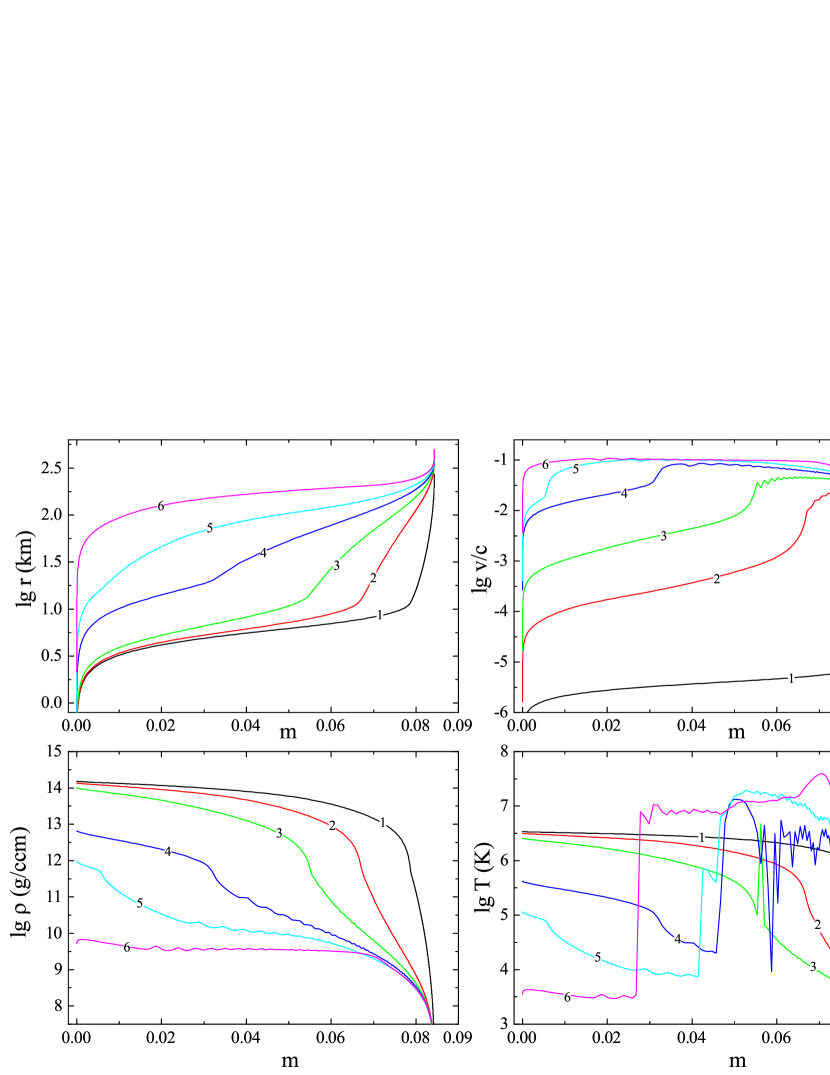
Figure 2: The first MMNS explosion period: from the equilibrium configuration (index 1) to the time of shock generation (index 6). The logarithms of the Eulerian coordinate $r$ (top left), the ratio $v/c$ (top right), the density (bottom left), and the temperature (bottom right) are shown as a function of the mass coordinate $m$.

The development of the explosion in the first period is shown in Fig. 2. It presents the distributions of the radius $r$, the ratio $v/c$, the density $\rho$, and the temperature $T$ as functions of the mass coordinate $m[M_{\odot}]$ for six times (the indices near the curves). On the graphs from the second to the fourth one the times corresponding to the indices are given in Table 1. The initial small velocity perturbation (time 1) corresponds to $v\propto r$. As can be seen, the evolution over times 1–6 leads to a flattening of the density and velocity distributions. Hydrodynamic disturbances (waves) are generated in this case, which are clearly seen, for example, on the velocity graphs at times 3 and 4 and in the density distributions 4–6. Propagating outward along a descending density profile, these disturbances transform into weak shock waves and lead to envelope heating, which is clearly seen on the temperature panel. By time 6 at a mass coordinate $m\approx 0.07$ evidence for the generation of a strong shock wave can be seen on the velocity and, especially, temperature graphs, which we will consider below.

Table 1. The times for the indices from 1 to 12 in Figs 2–4 Index 1 2 3 4 5 6 Time (s) 0.0 0.3110 0.3161 0.3191 0.3210 0.3236 Index 7 8 9 10 11 12 Time (s) 0.3252 0.3267 0.3292 0.3307 0.3573 0.6214

Figure 3: The second MMNS explosion period: shock breakout. The velocity $v$, density $\rho$, and temperature $T$ of the matter are shown as functions of the mass coordinate $m$.

The shock generation and breakout are shown in Fig. 3. The shock front and its propagation are clearly seen on the velocity panel (left). The shock passage through the envelope causes its temperature to rise by more than two orders of magnitude (right), reaching $T\sim 10^{10}$ K (i.e., $\sim 1$MeV). Furthermore, at shock breakout the outermost layers of the envelope are accelerated to ultrarelativistic velocities due to the cumulation effect (time 10 on the velocity graph). However, the fraction of the mass accelerated to $v/c\sim 1$ is extremely small (see Fig. 5 below and its discussion).

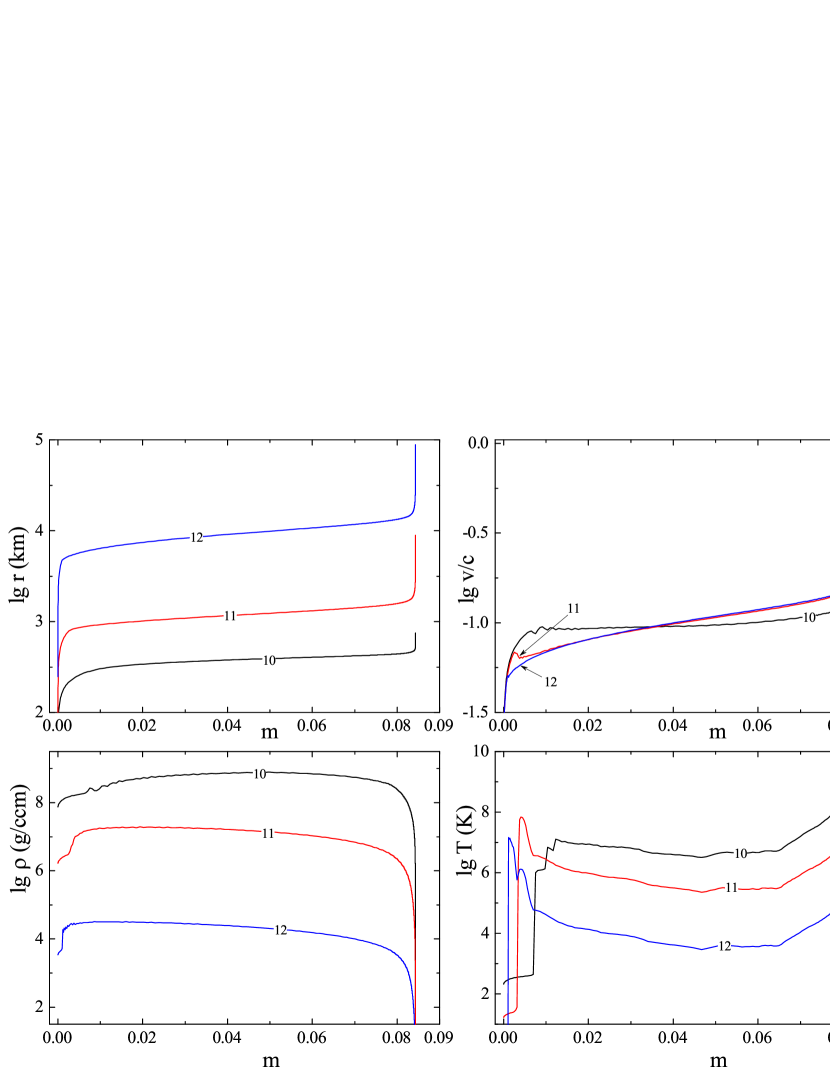
Figure 4: The third MMNS explosion period: from shock breakout to free expansion. The notation is the same as that in Fig. 2.

The third explosion period from shock breakout to the transition to free expansion is illustrated in Fig. 4. As can be seen, the star expands essentially at a density uniform in $m$. The velocity comes fairly rapidly to its final distribution (time 12). The temperature decreases monotonically virtually in the entire volume of the star, except for its inner part, where weak shocks lead to some additional heating.

DISCUSSION AND CONCLUSIONS

It is useful to compare the MMNS explosion parameters given above both with the original computation from Blinnikov et al. (1990) and with the computation in which an identical problem is solved within ordinary Newtonian hydrodynamics. Table 2 contains a comparison, where Blinn denotes the results from the mentioned 1990 paper, non-rel is the nonrelativistic case, and rel is the relativistic one.

Table 2. Comparison of the computational results for several approaches.

	Blinn	non-rel	rel
$M_{\mathrm{min}},\leavevmode\nobreak\ M_{\odot}$	0.095	0.089	0.084
$N_{\mathrm{zone}}$	151	2609	3899
$E_{\mathrm{exp}},\leavevmode\nobreak\ 10^{50}$ эрг	8.8	9.1	8.7

The first row $M_{\mathrm{min}}$ gives the mass of the exploding NS. The difference between our Newtonian computation and the computation by Blinnikov et al. (1990) is due to the use of different approximations for $P_{0}(\rho)$ and $E_{0}(\rho)$ (see Eqs. 44 and 45). The difference between non-rel and rel consists in using the Newtonian/ relativistic stellar equilibrium equations.

The number of zones $N_{\mathrm{zone}}$ in the Blinn computation is more than an order of magnitude smaller than that in our one. This did not allow one to provide a good resolution of the extended NS envelope and to correctly compute the cumulation of the shock during its breakout. That is why in this computation we did not run into the problem of $v/c>1$ discussed below.

Finally, the last row in the table gives the kinetic energy $E_{\mathrm{kin}}$ of the ejecta at the end of the computation. It can be seen that all three values are very close, while the differences between rel and non-rel are due mainly to the difference in the total masses (see also Fig. 5 below). On the whole, however, all three computations show a very similar picture of explosion development.

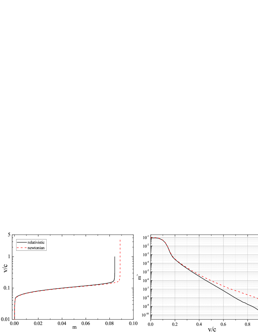
Figure 5: Comparison of the relativistic and Newtonian calculations. Left: The velocity distribution as a function of m at the final time. Right: The $m^{>}(v/c)$ distribution (for more details, see the text).

Let us now turn to the problem that gave rise to this paper. Figure 5 (left) shows the ejecta velocity distribution at the final time of our computations. As can be seen, in the nonrelativistic case part of the matter (though very small) was accelerated to $v/c>1$. Otherwise, however, the distributions are surprisingly similar.

Figure5 (right) shows the $m^{>}$ distribution as a function of the parameter $v/c$. By definition, $m^{>}(v/c)$ is the ejecta mass (in units of the solar mass) that has a velocity greater than $v/c$ at the final time of our computation. For example, the mass accelerated to $v/c>0.1$ is approximately $m^{>}\approx 0.047$ (i.e., almost half the entire stellar mass), while the mass accelerated to $v/c>0.2$ is already only $3\times 10^{-4}$. It can be seen from the same graph that the mass accelerated to $v/c>1$ in the nonrelativistic computation is $\sim 3\times 10^{-9}$. Note that the ejecta velocity distribution can be important for a comparison with the results of observations, in particular, for determining the properties of the so-called red and blue kilonovae for GRB170817A (Siegel 2019).

In conclusion, note that, on the whole, the MMNS explosion parameters derived by D.K. Nadyozhin in 1990 (Blinnikov et al. 1990) within the nonrelativistic approach agree well both with our results in the same approximation and with the completely relativistic computation (see, e.g., Table 2 and left part of Fig. 5). At the same time, it should be emphasized that in our computations we omitted several important points whose inclusion can affect the results obtained. First, the energy losses through neutrino radiation, for example, from electron–positron pair annihilation, become important in the region heated by the shock front with a temperature $T\sim 10^{10}$ K. These losses can reduce the cumulation effect and, accordingly, the ejecta velocity. This phenomenon is planned to be studied in the near future.

Second, during the disruption of a MMNS its matter experiences explosive decompression, which will be accompanied by numerous neutron-capture and beta-decay processes (r-process) leading to a significant change in the nuclear composition of the matter. At the same time, neutrinos are also emitted, but the energy of the corresponding nuclear transformations is released as well. Our preliminary offline computations (Panov and Yudin 2020) on fixed tracks show the promise and potential importance of these processes, which will undoubtedly also need to be studied in detail in future.

Third, it should be remembered that our formulation of the problem is idealized. In reality, a low-mass NS is a member of a binary system. As a result of mass transfer, it not only loses its mass, but is also heated due to the tidal interaction with its companion. In addition, as our preliminary computations show, the stability of the transfer process is lost not at $M_{2}=M_{\mathrm{min}}\sim 0.1M_{\odot}$, but at $M_{2}\sim 0.2M_{\odot}$. The star loses the rest of its mass on a fast hydrodynamic time scale, and the initial configuration for the MMNS explosion can differ noticeably from the spherically symmetric one already due to the influence of gravity from its massive companion (Manukovskii 2010). Computing the MMNS explosion in this formulation is a challenging three-dimensional problem that is of importance in its own right.

ACKNOWLEDGMENTS

This work was supported by the Russian Foundation for Basic Research (project no. 18-29-21019mk). Author is grateful to the anonymous referees whose remarks contributed significantly to an improvement of this paper.

APPENDIX: ENERGY CONSERVATION IN A STAR

The relativistic equations derived by us look unusual with regard to how the terms with the artificial viscosity $Q$ appear in them. Usually, the introduction of the latter is actually reduced to an additive to the pressure: $P\rightarrow P{+}Q$. In our case, however, there is also an additional contribution to the equation of motion (the last turn in (31)). Furthermore, the righthand side of the energy equation (24) is not reduced to the form $Q/\rho_{\mathrm{b}}^{2}(d\rho_{\mathrm{b}}/dt)$ because of the term $r^{3}$ under the logarithm. Let us demonstrate that, nevertheless, our formulas are quite self-consistent. We will work in the nonrelativistic limit. Let us multiply Eq. (31) by $v$ and integrate over $m_{\mathrm{b}}$ throughout the star. On the right we will obtain the term

$$\frac{1}{2}\int\frac{dv^{2}}{dt}dm_{\mathrm{b}}=\frac{dE_{\mathrm{kin}}}{dt},$$ (1)

i.e., the total time derivative of the kinetic energy. The gravitational acceleration (20) in the limit under consideration is simply $a_{\mathrm{G}}=-Gm_{\mathrm{b}}/r^{2}$. Its integral is

$$-\int\!\frac{vGm_{\mathrm{b}}dm_{\mathrm{b}}}{r^{2}}=\int\!\frac{d}{dt}\!\left(\frac{1}{r}\right)Gm_{\mathrm{b}}dm_{\mathrm{b}}=-\frac{dE_{\mathrm{grav}}}{dt},$$ (2)

where $E_{\mathrm{grav}}$ is the gravitational energy. We integrate the next term in (31) by parts:

$$-\int\!4\pi r^{2}v\frac{\partial(P{+}Q)}{\partial m_{\mathrm{b}}}dm_{\mathrm{b}}=\int\!(P{+}Q)\frac{d}{dt}\!\left(\!\frac{1}{\rho_{\mathrm{b}}}\!\right)dm_{\mathrm{b}}.$$ (3)

The energy equation (24) can be rewritten in an equivalent form:

$$(P+Q)\frac{d}{dt}\!\left(\!\frac{1}{\rho_{\mathrm{b}}}\!\right)=-\frac{dE}{dt}+\frac{3Qv}{r\rho_{\mathrm{b}}}.$$ (4)

Substituting this expression into (3) , we will find that the second term on the right in (4) is canceled out with the last term in the equation of motion (31) during its integration. There remains only the total derivative of the star’s internal energy $E_{\mathrm{int}}=\int\!Edm_{\mathrm{b}}$. Thus,we obtained the law of conservation of the star’s total energy in the form $dE_{\mathrm{tot}}/dt=0$, where$E_{\mathrm{tot}}=E_{\mathrm{kin}}+E_{\mathrm{grav}}+E_{\mathrm{int}}$.

REFERENCES

1.   B.P. Abbott et al., Astroph. J. Lett., 848, L:12 (2017)

2.   S.I. Blinnikov, I.D. Novikov, T.V. Perevodchikova, A.G. Polnarev, Sov. Astron. Lett. 10 177 (1984)

3.   Blinnikov S.I., Imshennik V.S., Nadyozhin D.K., Novikov I.D., Perevodchikova T.V., Polnarev A.G., Sov. Astron. 34 595 (1990)

4.   S.I. Blinnikov, D.K. Nadyozhin, N.I. Kramarev, and A.V. Yudin, Astron. Rep. 65, 385 (2021)

5.   S. Weinberg, Gravity and Cosmology: Principles and Applications of the General Theory of Relativity, Wiley-VCH, Weinheim, (1972)

6.   Clark J.P.A., Eardley D.M., Astroph. J. 215 311-322 (1977)

7.   Liebendoerfer, M; Mezzacappa, A.; Thielemann, K.-F., Phys. Rev. D, 63, 104003 (2001)

8.   K.V. Manukovskii, Astron. Lett., 36, 3, 191–203 (2010)

9.   I.V. Panov and A.V. Yudin, Astron. Lett. 46, 518 (2020)

10.   D.M. Siegel, European Phys. J. A 55, 203 (2019)

11.   Sumiyoshi K., Yamada S., Suzuki H., Hillebrandt W., Astron. Astrophys. 334, 159-168 (1998)

12.   Hwang, J.; Noh, H., Astrophys. J., 833, 2, 180, 12 pp. (2016)

13.   P. Haensel, A.Y. Potekhin, D.G. Yakovlev, ‘‘Neutron Stars 1: Equation of State and Structure’’, Springer, New York (2007)

14.   Haensel, P., Potekhin A.Y., Astron. Astroph., 428, 191-197 (2004)