Abstract

We consider the Seiberg-Witten solution of pure $\mathcal{N}=2$ gauge theory in four dimensions, with gauge group $SU(N)$. A simple exact series expansion for the dependence of the $2(N-1)$ Seiberg-Witten periods $a_{I}(u),a_{DI}(u)$ on the $N-1$ Coulomb-branch moduli $u_{n}$ is obtained around the $\mathbb{Z}_{2N}$-symmetric point of the Coulomb branch, where all $u_{n}$ vanish. This generalizes earlier results for $N=2$ in terms of hypergeometric functions, and for $N=3$ in terms of Appell functions. Using these and other analytical results, combined with numerical computations, we explore the global structure of the Kähler potential $K=\frac{1}{2\pi}\sum_{I}\text{Im}(\bar{a}_{I}a_{DI})$, which is single valued on the Coulomb branch. Evidence is presented that $K$ is a convex function, with a unique minimum at the $\mathbb{Z}_{2N}$-symmetric point. Finally, we explore candidate walls of marginal stability in the vicinity of this point, and their relation to the surface of vanishing Kähler potential.

1 Introduction

1.1 An Expansion for the $SU(N)$ Seiberg-Witten Periods

The Seiberg-Witten (SW) solution of $\mathcal{N}=2$ $SU(2)$ gauge theory in four dimensions [1, 2] and its generalizations have led to many new insights into the dynamics of gauge theories and string theories at strong coupling. In the original work [1], the exact low-energy effective Lagrangian on the Coulomb branch of the pure $SU(2)$ gauge theory was determined by computing the periods of a suitable SW one-form over the homology cycles of an auxiliary genus-one Riemann surface – the SW curve.

In this paper, we revisit the generalization of the SW solution to pure $SU(N)$ gauge theory [3, 4, 5], beginning with a brief sketch of its salient features. These theories have a Coulomb branch that is parameterized by $N-1$ complex coordinates $u_{n}$, $n=0,\ldots,N-2$, in correspondence with the gauge-invariant products of the $SU(N)$ vector multiplet scalars. At generic points on the Coulomb branch, the low-energy theory on the Coulomb branch is a $U(1)^{N-1}$ gauge theory described by $N-1$ abelian ${\cal N}=2$ vector multiplets $A_{I}$, $I=1,\cdots,N-1$, whose complex scalar bottom components we denote by $a_{I}$. Note that the $a_{I}(u)$ are locally (but not globally) holomorphic functions of the Coulomb branch moduli.

The leading long-distance interactions of these vector multiplets are completely determined if we also specify $N-1$ locally holomorphic functions $a_{DI}(u)$, which can be thought of as vector multiplet scalars in a magnetic dual description. Then the Kähler potential describing the sigma model for the scalars is given by

$$K={i\over 4\pi}\sum_{I=1}^{N-1}\Big{(}a_{I}\,\bar{a}_{DI}-\bar{a}_{I}\,a_{DI}\Big{)}\,,$$ (1.1)

while the symmetric matrix of complexified $U(1)^{N-1}$ gauge couplings is given by $\tau_{IJ}={\partial a_{DI}/\partial a_{J}}$. It follows from ${\cal N}=2$ supersymmetry that the positive-definite Kähler metric $g_{I{J}}={\partial^{2}K}/\partial a^{I}\partial\bar{a}^{J}$ is (up to a positive constant) the same as the imaginary part of $\tau_{IJ}$.

The SW solution can be expressed through the $2(N-1)$ special coordinates $a_{I}(u),a_{DI}(u)$ (also called SW periods), which in turn are identified with the periods of a meromorphic one-form $\lambda$ on a canonical basis of homology cycles $(\mathfrak{A}_{I},\mathfrak{B}_{I})$ of a genus $N-1$ hyperelliptic curve ${\cal C}(u)$ that depends on the moduli,

$$2\pi i\,a_{I}=\oint_{\mathfrak{A}_{I}}\lambda\,,\qquad 2\pi i\,a_{DI}=\oint_{\mathfrak{B}_{I}}\lambda\,.$$ (1.2)

The derivatives of the SW differential with respect to the moduli $u_{n}$ are holomorphic one-forms, which is sufficient to ensure the positivity of the Kähler metric. Different choices of homology basis $(\mathfrak{A}_{I},\mathfrak{B}_{I})$ act on the special coordinates as electric-magnetic duality transformations: a change of homology basis by $M\in\text{Sp}(2(N-1),\mathbb{Z})$ preserves the canonical intersection pairing, while the period vector $v=(a_{DI},a_{I})$ transforms under such a duality transformation in the doublet representation.

The presentation of the $SU(N)$ SW solution sketched above is deceptively simple: obtaining explicit, tractable expressions for the periods that are valid in varied regions of moduli space is in general a formidable challenge. For gauge group $SU(2)$, the periods are elliptic integrals and can be expressed in terms of Gauss hypergeometric functions [1]. The latter have well-known analytic continuations in the entire $u$-plane. For general $N$, efficient methods for obtaining the period integrals in certain limits have been developed in [6, 7, 8, 9, 10, 11, 12]. The $SU(N)$ periods are known to satisfy Picard-Fuchs differential equations as functions of the moduli $u_{n}$ [5, 13] (see also [14, 15]). For $SU(3)$ gauge group, the solutions to these Picard-Fuchs equations were shown in [5] to be given by Appell $F_{4}$ functions. However, the complexity of the Picard-Fuchs equations increases rapidly with $N$.

A principal result of this paper is the derivation of a simple, exact series expansion for the $a_{I},a_{DI}$ periods around the origin of moduli space, where all $u_{n}$ vanish, generalizing the earlier results for $N=2$ and $N=3$. This result is expressed as Theorem 2.1 below; it is then refined in several Corollaries and exploited in various applications. For $SU(2)$ and $SU(3)$ gauge groups, our series expansion reduces to the known hypergeometric and Appell function representations, respectively. For higher $N$, it takes the form of a series expansion in the moduli $u_{n}$, which is optimal in the sense that the coefficient of each monomial $u_{0}^{\ell_{0}}\cdots u_{N-2}^{\ell_{N-2}}$ consists of a single factorized term.

1.2 Exploring the $SU(N)$ Kähler Potential

In addition to the SW periods $a_{I},a_{DI}$ themselves, another object whose properties we wish to illuminate is the Kähler potential (1.1). Besides being an important ingredient in the low-energy Lagrangian, our interest in the Kähler potential $K$ derives from the observation [16] that $K$ plays a critical role in a certain supersymmetry-breaking scenario that connects four-dimensional ${\cal N}=2$ Yang-Mills theory with gauge group $G$ to a non-supersymmetric $G$ gauge theory with two Weyl fermions transforming in the adjoint representation of $G$ – in short, $N_{f}=2$ adjoint QCD. The renormalization group flow from the supersymmetric to the non-supersymmetric theory is triggered by the soft supersymmetry-breaking deformation $\mathcal{T}_{\text{UV}}\sim\text{Tr}(\bar{\phi}\phi)$, which gives mass to the complex ${\cal N}=2$ vector multiplet scalars. Crucially, the operator $\mathcal{T}_{\text{UV}}$ is the bottom component of the protected ${\cal N}=2$ stress-tensor supermultiplet; it can therefore be reliably tracked to the low-energy description on the Coulomb branch, where it is identified with the Kähler potential, i.e. $\mathcal{T}_{\text{UV}}\rightarrow\mathcal{T}_{\text{IR}}\sim K$. Several comments are in order:

• Since ${\cal T}_{\text{UV}}$ is a well-defined operator and it flows to $K$ in the IR, it follows that the Kähler potential given by (3.1) is a well-defined function on the Coulomb branch, i.e. it does not suffer from the usual Kähler ambiguities, and it is invariant under $\text{Sp}(2(N-1),{\mathbb{Z}})$ electric-magnetic duality transformations.

• Even though $\mathcal{T}_{\text{UV}}\sim\text{Tr}(\bar{\phi}\phi)$ is classically positive-definite, quantum effects can render its expectation value negative. Indeed we show below that there is a region of the Coulomb branch – which we term the strong-coupling region – where $K<0$. Note that this region is well defined, because $K$ is well defined (see (i) above).

• The deformation by ${\cal T}_{\text{UV}}$ leads to a supersymmetry-breaking scalar potential proportional to $K$ on the Coulomb branch. In this way, the properties of $K$ lead to a prediction for the vacuum structure of non-supersymmetric $N_{f}=2$ adjoint QCD, which is reliable if the supersymmetry-breaking mass scale is small compared to the strong coupling scale $\Lambda$ of the ${\cal N}=2$ theory. In upcoming work [19], we utilize this perspective to explore the phases of $N_{f}=2$ adjoint QCD with gauge group $SU(N)$.

With the preceding motivation in mind, we here apply our explicit and (relatively) simple expressions for the SW periods, along with other analytic and numeric methods, to study the global structure of the SW Kähler potential $K$, focusing on its stationary points and convexity properties. For the case of gauge group $SU(2)$, $K(u)$ is a convex function of the single complex modulus $u$, with a single minimum at the origin $u=0$ of moduli space. This minimum is depicted in figure 1, and was also previously discussed in [20, 16] in the context of supersymmetry-breaking.

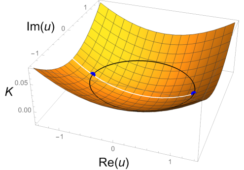
Figure 1: The Kähler potential for gauge group $SU(2)$ in the complex $u$-plane (with $\Lambda=1$), made using the hypergeometric function representation of the periods (see section 2.4). The black curve indicates the $K=0$ contour; it is the boundary of the strong-coupling region where $K<0$. Note that the monopole and dyon points (indicated by the blue dots) lie on this $K=0$ boundary.

For general $N>2$, $K$ is a function of $N-1$ complex variables, and the extraction of its properties is considerably more involved. We prove that for general $N$, the origin of moduli space where all $u_{n}=0$ is a stationary point (see section 4.3). Since the SW curve is invariant under a $\mathbb{Z}_{2N}$ symmetry when all the $u_{n}=0$ – corresponding to the action of the unbroken $\mathbb{Z}_{4N}$ $R$-symmetry on the moduli space – we refer to this point as the $\mathbb{Z}_{2N}$-symmetric point (or simply the ${\mathbb{Z}}_{2N}$ point). We compute the value $K(0)$ at the $\mathbb{Z}_{2N}$-symmetric point and show that it is negative, scaling with $N$ as $K(0)\sim-N^{2}$ (and given explicitly in (3.10)). Then, much as in $SU(2)$, there is a region around the origin for which $K$ is negative, $K<0$, which we refer to as the strong coupling region. The boundary of this region for $SU(2)$ is depicted by the black curve in figure 1, which contains the singular monopole and dyon points. For general $N$, the $N$ multi-monopole points – the $N>2$ generalization of the monopole and dyon points studied in [21] – also lie on the $K=0$ boundary of this region. In section 5.4 we numerically study this $K=0$ surface for the case of gauge group $SU(3)$, slices of which are depicted in figures 4(a) and 4(b).

It is natural to conjecture that the origin is the unique global minimum of the Kähler potential, and that $K$ is everywhere convex, for all $N$. While this conjecture is as of yet proven only for gauge group $SU(2)$, it is supported by the following evidence that we present throughout the paper:

• If $K$ has another stationary point, it occurs at a negative value of $K$, i.e. within the strong coupling region. The proof of this statement is given in section 4.1. Thus one may restrict the search for another minimum to this region.

• For gauge group $SU(3)$, we have thoroughly explored the Kähler potential numerically. This analysis is presented in section 5.4. Our numerical studies have shown $K$ to be convex on every slice upon which we have evaluated it, with no evidence for a minimum away from the ${\mathbb{Z}}_{2N}$-symmetric point at the origin.

• We obtain some partial analytic results that are valid for all $N$ and consistent with the convexity conjecture. For instance, on the slice parameterized by a single modulus $u_{0}$ (with all other $u_{n}=0$) there is no stationary point for $\text{Im}(u_{0})\neq 0$ (see section 4.4).

It would be interesting to find a definitive proof (or disproof) of this conjecture, but we leave this problem for the future.

1.3 Charting Candidate Curves of Marginal Stability

It has been known since [1] that there are walls of marginal stability on the Coulomb branch. In the simplest cases, such walls are loci where a massive BPS particle becomes marginally unstable to decay into two (or more) other BPS particles – or conversely, loci where two (or more) BPS particles can form threshold bound states. This occurs when the complex central charges of the BPS particles in question, which are determined by the SW periods, have aligned phases. The $SU(2)$ case was completely understood in [1, 22]: a wall of marginal stability separates the moduli space into a strong-coupling chamber around the origin, and a weak-coupling chamber extending out to infinity. This wall precisely coincides with the black $K=0$ contour depicted in figure 1, i.e. the $SU(2)$ strong-coupling chamber for massive BPS states is the same as our strong-coupling region defined by $K<0$.

Already the case of $SU(3)$ gauge group is much richer, see for instance [23, 24, 25] for discussions specifically focusing on this case, with many additional references to the large literature on BPS states and wall crossing in 4d ${\cal N}=2$ theories.

As another application of our formulas for the SW periods of $SU(N)$ gauge theory, in section 6 we map out some candidate walls of marginal stability within the strong coupling $K<0$ region near the origin of the Coulomb branch. We emphasize that the scope of our analysis is narrow: we do not claim to find all walls of marginal stability, nor do we analyze the much more delicate question of which BPS states actually decay or form bound states as we cross these walls. The results in this section should be viewed as motivation for a more detailed study of this problem.

Outline

The remainder of this paper is organized as follows:

In section 2 we present a simple series expansion for the $SU(N)$ SW periods around the $\mathbb{Z}_{2N}$-symmetric point at the origin of moduli space, as well as various simplifications of this expression for different special values of the moduli, and for low values of $N$. The proof of the main theorem is relegated to appendix A, and the proof that the expansion reproduces the $SU(3)$ Appell functions appears in appendix B.

In section 3 we build on these results to express the Kähler potential in a simple diagonal form. We evaluate $K$ at the ${\mathbb{Z}}_{2N}$-symmetric point, showing that it behaves (up to an ${\cal O}(1)$ positive coefficient) as $-N^{2}$ for $N\gg 1$, and additionally discuss the structure of the Kähler potential for restricted values of the moduli.

In section 4 we collect a number of general results regarding the structure of the Kähler potential, including a proof that the ${\mathbb{Z}}_{2N}$-symmetric point is a stationary point (as expected from the ${\mathbb{Z}}_{2N}$-symmetry), and that $K$ is negative at an arbitrary stationary point. We also re-express the derivatives of $K$ with respect to the moduli as two-real-dimensional integrals, which is useful both for proving some of the results in this section, and for numerical computations in later sections.

In section 5 we restrict to the case of gauge group $SU(3)$. By mapping the SW curve and differential to an elliptic problem, we compute the SW periods on the cusp slice of moduli space, where the discriminant of the curve vanishes – and which includes both the multi-monopole and the Argyres-Douglas [26] points of $SU(3)$. We use these results to evaluate $K$ at special points of the moduli space. Next, we describe the results of a numerical exploration of $K$, presenting evidence that the Kähler potential is convex and that the ${\mathbb{Z}}_{2N}$-symmetric point at the origin is the only minimum. Appendix C includes a brief review of elliptic functions and modular forms as needed for the analysis of this section, and numerical methods for evaluating $K$ are discussed in appendix D.

In section 6 we investigate candidate walls of marginal stability within the $K<0$ strong-coupling region. We mostly focus on special slices of $SU(3)$ moduli space, but also present some results for general $N$. A summary of the BPS particles that are stable in the strong-coupling chamber of the $SU(N)$ theory (with emphasis on the case $N=3$) appears in appendix E.

Acknowledgements

The research of ED is supported in part by the National Science Foundation under grants PHY-19-14412 and PHY-22-09700. The research of EN is supported by World Premier International Research Center Initiative (WPI), MEXT, Japan. EN also acknowledges the Aspen Center for Physics where part of this work was performed, which is supported by National Science Foundation grant PHY-1607611. TD is supported by a DOE Early Career Award under DE-SC0020421, by the Simons Collaboration on Global Categorical Symmetries, and by the Mani L. Bhaumik Presidential Chair in Theoretical Physics at UCLA. We are grateful to P. Dumitrescu, A. Neitzke, and F. Yan for useful discussions. We especially thank E. Gerchkovitz for collaboration and discussion on closely related work [12, 19].

2 Expanding the Periods around the ${\mathbb{Z}}_{2N}$ Point

In this section we analyze the SW periods in the vicinity of the ${\mathbb{Z}}_{2N}$-symmetric SW curve, or equivalently the ${\mathbb{Z}}_{2N}$-symmetric origin, where all $u_{n}=0$, of the Coulomb branch.

2.1 Seiberg-Witten Review

We consider pure ${\cal N}=2$ supersymmetric Yang-Mills theory with gauge group $SU(N)$ (for any $N\geq 2$) and no hypermultiplets in four space-time dimensions. We begin by briefly reviewing the Seiberg-Witten (SW) solution for this class of theories, which was found in [1, 3, 4, 5]. This solution determines the vector multiplet scalars $a_{I}(u)$ and their magnetic duals $a_{DI}(u)$ as locally holomorphic functions of the gauge invariant Coulomb branch moduli $u_{n}~{}(n=0,1,\ldots,N-2)$. This is accomplished by expressing them as periods of a meromorphic SW one-form (or differential) $\lambda$ over a canonical basis of homology one-cycles $\mathfrak{A}_{I}$ and $\mathfrak{B}_{I}$,

$$2\pi i\,a_{I}=\oint_{\mathfrak{A}_{I}}\lambda\,,\hskip 65.76596pt2\pi i\,a_{DI}=\oint_{\mathfrak{B}_{I}}\lambda\,.$$ (2.1)

on a family of curves ${\cal C}(u)$ (known as SW curves) that depend holomorphically on the moduli $u_{n}$. Recall that, given a compact, oriented surface a canonical homology basis of oriented one-cycles $(\mathfrak{A}_{I},\mathfrak{B}_{I})$ is defined by the following intersection pairings,

$$\#(\mathfrak{A}_{I},\mathfrak{B}_{J})=\delta_{IJ}~{},\qquad\#(\mathfrak{A}_{I},\mathfrak{A}_{J})=0~{},\qquad\#(\mathfrak{B}_{I},\mathfrak{B}_{J})=0~{},$$ (2.2)

where $\#(X,Y)=-\#(Y,X)$ denotes the antisymmetric intersection pairing of the oriented one-cycles $X$ and $Y$.

It is standard to introduce a locally defined and holomorphic prepotential ${\cal F}(a)$, which captures the relationship between the electric and magnetic periods $a_{I}(u)$ and $a_{DI}(u)$, as well as the symmetric matrix $\tau_{IJ}(u)$ of effective holomorphic $U(1)^{N-1}$ gauge couplings on the Coulomb branch,

$$a_{DI}={\partial{\cal F}\over\partial a_{I}}~{},\qquad\tau_{IJ}={\partial a_{DI}\over\partial a_{J}}={\partial^{2}{\cal F}\over\partial a_{I}\partial a_{J}}=\tau_{JI}~{},\qquad(I,J=1,\cdots,N-1)~{}.$$ (2.3)

The SW curve ${\cal C}(u)$ is parametrized by the $N-1$ complex moduli $u_{0},\cdots,u_{N-2}$. For each value of the $u_{n}$, the curve is hyper-elliptic and can be chosen to take the following form,

$$y^{2}=A(x)^{2}-\Lambda^{2N}\,,\hskip 57.81621ptA(x)=x^{N}-\sum_{n=0}^{N-2}u_{n}x^{n}\,,$$ (2.4)

where $\Lambda$ is the strong-coupling scale of the non-Abelian gauge theory. For the remainder of this paper we set $\Lambda=1$, so that all quantities are dimensionless. In terms of the data in (2.4), the SW differential $\lambda$ is given by

$$\lambda={xA^{\prime}(x)dx\over y}\,.$$ (2.5)

By construction, the derivatives of the SW differential $\lambda$ with respect to the moduli $u_{n}$ produce holomorphic Abelian differentials, modulo exact differentials,

$${\partial\lambda\over\partial u_{n}}=\omega_{n}-dx{\partial\over\partial x}\left({x^{n+1}\over\sqrt{A(x)^{2}-1}}\right)\,,\hskip 36.135pt\omega_{n}={x^{n}dx\over\sqrt{A(x)^{2}-1}}~{}.$$ (2.6)

Here the $\omega_{n}$ (with $n=0,\ldots,N-2$) are holomorphic Abelian differentials of the first kind, which furnish a basis for the Dolbeault cohomology $H^{(1,0)}({\cal C}(u),{\mathbb{C}})$. It follows that the matrix $\tau_{IJ}(u)$ is the period matrix of the curve ${\cal C}(u)$ for a given set of $u_{n}$. By the Riemann bilinear relations, $\tau_{IJ}(u)$ is symmetric and has positive definite imaginary part, as required for a matrix of complexified $U(1)^{N-1}$ gauge couplings in a unitary theory.

2.2 The ${\mathbb{Z}}_{2N}$-Symmetric Curve

The Seiberg-Witten curve ${\cal C}(0)$ at the origin of the Coulomb branch, obtained by setting all $u_{n}=0$ in (2.4), is given by

$$y^{2}=x^{2N}-1~{}.$$ (2.7)

Note that ${\cal C}(0)$ is manifestly invariant under the following ${\mathbb{Z}}_{2N}$ transformation,

$$(x,y)\to(\varepsilon x,\pm y)~{},\qquad\varepsilon=e^{\frac{2\pi i}{2N}}~{},$$ (2.8)

with $\varepsilon$ a $2N$-th root of unity. This symmetry descends from a physical $\mathbb{Z}_{4N}$ discrete $R$-symmetry of the ${\cal N}=2$ gauge theory, whose quotient by fermion parity $(-1)^{F}$ acts on the bosonic moduli space coordinates $u_{n}$ via the following ${\mathbb{Z}}_{2N}$ action,

$$u_{n}\;\to\;e^{\frac{2\pi i(N-n)}{2N}}u_{n}~{}.$$ (2.9)

Thus the origin, where all $u_{n}=0$, is the unique point on the Coulomb branch where this ${\mathbb{Z}}_{2N}$ symmetry is unbroken. For this reason we refer to ${\cal C}(0)$ as the ${\mathbb{Z}}_{2N}$-symmetric curve.

The branch points of ${\cal C}(0)$ are the $2N$ roots of unity $\varepsilon^{n}$, with $n=0,\cdots,2N-1$, and the branch cuts in the hyper-elliptic representation may be chosen to lie along the intervals $[\varepsilon^{2I-2},\varepsilon^{2I-1}]$ with $I=1,\cdots,N$. We define the cycles $\mathfrak{A}_{I}$ and $\mathfrak{B}_{I}$ (with $I=1,\cdots,N$) as follows,

$$\mathfrak{A}_{I}=\bigcup_{J=1}^{I}\hat{\mathfrak{A}}_{J}\,,\hskip 50.58878pt\hat{\mathfrak{A}}_{I}=(\varepsilon^{2I-2},\varepsilon^{2I-1})\,,\hskip 50.58878pt\mathfrak{B}_{I}=(\varepsilon^{2I-1},\varepsilon^{2I})~{}.$$ (2.10)

Here the intervals indicating the cycles are somewhat schematic. In truth, the cycles are closed curves surrounding the branch points, as indicated in detail in figure 2 for the case $N=3$. Crucially, we choose the orientations of the cycles as indicated in the figure: clockwise for $\hat{\mathfrak{A}}_{J}$, $\mathfrak{A}_{I}$ and counter-clockwise for $\mathfrak{B}_{I}$. This ensures that $\mathfrak{A}_{I}$ and $\mathfrak{B}_{I}$ comprise a canonical homology basis in the sense of (2.2).

Warning: The cycles $\mathfrak{A}_{I}$ and $\mathfrak{B}_{I}$ defined above (which are very convenient near the origin) do not coincide with other common duality frames used in SW theory, e.g. the standard electric frame that is simply related to the UV theory by Higgsing (and that, in a suitable sense, becomes weakly coupled at infinity in the moduli space), or the standard magnetic frame that becomes weakly-coupled at the multi-monopole point where the maximal number of mutually local monopoles become massless. Rather, our $\mathfrak{A}_{I}$ and $\mathfrak{B}_{I}$ cycles are related to these bases by an electric-magnetic duality transformation. We will see this explicitly below.

Figure 2: Branch points $x=\varepsilon^{n}$ for the ${\mathbb{Z}}_{2N}$-symmetric curve $y^{2}=x^{2N}-1$ for the special case $N=3$, for which $\varepsilon=e^{2\pi i/6}$. The branch cuts are denoted by black double lines, while the $\hat{\mathfrak{A}}_{J}$ and $\mathfrak{B}_{I}$ cycles defined above are shown in blue and red, respectively. The integration paths used to define the function $Q(\xi)$ (see (2.13) below) are shown in green.

Note that the $N$ pairs of $\mathfrak{A}$- and $\mathfrak{B}$-cycles defined above are not independent: the union of all $\mathfrak{A}$-cycles is homologically trivial, and so is the union of all $\mathfrak{B}$-cycles. Via (2.1), this translates into

$$\sum_{I=1}^{N}a_{I}=\sum_{I=1}^{N}a_{DI}=0\,,$$ (2.11)

as required in $SU(N)$ gauge theory.

2.3 Expanding Around the ${\mathbb{Z}}_{2N}$-Symmetric Curve

Given the conventions spelled out above, the periods $a_{I}(u)$, $a_{DI}(u)$ (with $I=1,\cdots,N-1$) can be expressed as follows,

$$a_{I}=\sum_{J=1}^{I}\big{\{}Q(\varepsilon^{2J-1})-Q(\varepsilon^{2J-2})\big{\}}~{},\qquad a_{DI}=Q(\varepsilon^{2I})-Q(\varepsilon^{2I-1})~{},\qquad\varepsilon=e^{\frac{2\pi i}{2N}}~{}.$$ (2.12)

Here $Q(\xi)$ is a function on the $2N$-th roots of unity $\xi$ (i.e. $\xi^{2N}=1$), which is defined as the integral of the SW differential $\lambda$ in (2.5) along a path from $x=0$ to $x=\xi$ (i.e. one of the green paths in figure 2),

$$\pi i\,Q(\xi)=\int_{0}^{\xi}\lambda~{}.$$ (2.13)

As usual, the factors of 2 in (2.12) account for the fact that the integral over a full cycle is twice the integral over the corresponding interval on a single sheet of the curve.

The function $Q(\xi)$ is a hyper-elliptic integral whose series expansion in powers of the moduli $u_{n}$ is given by the following theorem:

Theorem 2.1

The function $Q(\xi)$ has the following series expansion around $u_{n}=0$,

$$Q(\xi)=\sum_{{\{\ell_{n}\}=0\atop n=0,\ldots,N-2}}^{\infty}V_{L,M}(\xi)\,{u_{0}^{\ell_{0}}\cdots u_{N-2}^{\ell_{N-2}}\over\ell_{0}!\,\cdots\ell_{N-2}!}~{},\qquad L=\sum_{j=0}^{N-2}j\ell_{j}~{},\qquad M=\sum_{j=0}^{N-2}\ell_{j}~{},$$ (2.14)

where the coefficients $V_{L,M}(\xi)$ are given by,

$$V_{L,M}(\xi)={2^{M-(L+1)/N}\over 2\pi^{2}N}\,\xi^{NM+L+N+1}\Gamma(\tfrac{L+1}{N})\Gamma(\tfrac{NM-L-1}{2N})^{2}\sin^{2}\big{(}\pi\tfrac{NM-L-1}{2N}\big{)}\,.$$ (2.15)

The proof of this theorem is essentially calculational; we defer the details to appendix A. Note that the resulting series expansion is optimal, i.e. the coefficient of each monomial $u_{0}^{\ell_{0}}\cdots u_{N-2}^{\ell_{N-2}}$ consists of a single factorized term. The following corollaries are direct consequences of Theorem 2.1.

Corollary 2.2

The summation over $\ell_{0}$ may be carried out to express $Q(\xi)$ in terms of an infinite series of Gauss hypergeometric functions $F(a,b;c;z)={}_{2}F_{1}(a,b;c;z)$,

$$Q(\xi)=\sum_{\ell_{1},\ldots,\ell_{N-2}=0}^{\infty}{2^{M_{0}-(L+1)/N}\,\over 2\pi^{2}N}\,\xi^{NM_{0}+L+N+1}\,\Gamma(\tfrac{L+1}{N})\,Y_{M_{0}}(\xi^{N},L)\,{u_{1}^{\ell_{1}}\cdots u_{N-2}^{\ell_{N-2}}\over\ell_{1}!\,\cdots\ell_{N-2}!}~{},$$ (2.16)

where $L=\sum_{j=0}^{N-2}j\ell_{j}$ and $M_{0}=\sum_{j=1}^{N-2}\ell_{j}$, while the coefficients $Y_{M_{0}}(\xi^{N},L)$ are given by

$$Y_{M_{0}}(\xi^{N},L) = 2u_{0}\,\xi^{N}\cos^{2}\big{(}\pi\tfrac{NM_{0}-L-1}{2N}\big{)}\Gamma(\tfrac{NM_{0}+N-L-1}{2N})^{2}F\left(\tfrac{NM_{0}+N-L-1}{2N},\,\tfrac{NM_{0}+N-L-1}{2N};\,\tfrac{3}{2};\,u_{0}^{2}\right)$$ (2.17)

$$+\sin^{2}\big{(}\pi\tfrac{NM_{0}-L-1}{2N}\big{)}\Gamma(\tfrac{NM_{0}-L-1}{2N})^{2}\,F\left(\tfrac{NM_{0}-L-1}{2N},\,\tfrac{NM_{0}-L-1}{2N};\,{\tfrac{1}{2}};\,u_{0}^{2}\right)\,.$$

Corollary 2.3

In the special case where $u_{n}=0$ for all $n\not=0$, the function $Q(\xi)$ is given by a linear combination of Gauss hypergeometric functions $Q(\xi)=\xi Q_{1}+\xi^{N+1}Q_{N+1}$, with

$$Q_{1} = {u_{0}\,\Gamma(1+\tfrac{1}{2N})\over 2\,\Gamma(\tfrac{3}{2})\,\Gamma({1\over 2}+\tfrac{1}{2N})}\,F\big{(}\tfrac{N-1}{2N},\tfrac{N-1}{2N};\tfrac{3}{2};u_{0}^{2}\big{)}\,,$$

$$Q_{N+1} = {\Gamma({\tfrac{1}{2}}+\tfrac{1}{2N})\over 2\,\Gamma(\tfrac{1}{2})\,\Gamma(1+\tfrac{1}{2N})}\,F\big{(}-\tfrac{1}{2N},-\tfrac{1}{2N};{\tfrac{1}{2}};u_{0}^{2}\big{)}\,.$$ (2.18)

The proof of these corollaries, using the results of Theorem 2.1 as well as the standard series representation of $F(a,b;c;z)$, is essentially straightforward and left to the reader. Note that while the hypergeometric functions appearing in these corollaries may be analytically continued to all values of $u_{0}$, it is in general not clear how this affects the convergence of the resulting series expansions.

2.4 Comparison to known $SU(2)$ results

When $N=2$, the only modulus is $u_{0}$. Then (2.12) (with $\varepsilon=i$) together with Corollary 2.3 implies that

$$a = Q(i)-Q(1)=(i-1)Q_{1}-(i+1)Q_{3}~{},$$

$$a_{D} = Q(-1)-Q(i)=-(1+i)Q_{1}-(1-i)Q_{3}~{},$$ (2.19)

where the functions $Q_{1}$ and $Q_{3}$ are defined in Corollary 2.3 by,

$$Q_{1}(u_{0}) = {u_{0}\Gamma({5\over 4})\over 2\Gamma({3\over 2})\Gamma({3\over 4})}F(\tfrac{1}{4},\tfrac{1}{4};\tfrac{3}{2};u_{0}^{2})~{},$$

$$Q_{3}(u_{0}) = {\Gamma({3\over 4})\over 2\Gamma({1\over 2})\Gamma({5\over 4})}F(-\tfrac{1}{4},-\tfrac{1}{4};\tfrac{1}{2};u_{0}^{2})~{}.$$ (2.20)

Note that these functions have two symmetric branch cuts running from $u_{0}=\pm 1$ to $u_{0}=\pm\infty$ along the real axis.

Let us compare this to the $SU(2)$ periods determined by Seiberg and Witten (SW) in [1, 2]; we will follow the conventions of their [2]. Taking into account an overall factor of $\sqrt{2}$ that results from differently normalized strong coupling scales ($\Lambda_{\text{us}}=\sqrt{2}\Lambda_{\text{SW}}$, as in footnote 4), we obtain,

$$a_{\text{SW}}(u_{0}) = \sqrt{1+u_{0}}\,F(-\tfrac{1}{2},\tfrac{1}{2};1;\tfrac{2}{1+u_{0}})~{},$$

$$a_{D,\text{SW}}(u_{0}) = {i(u_{0}-1)\over\sqrt{2}}\,F(\tfrac{1}{2},\tfrac{1}{2};2;\tfrac{1-u_{0}}{2})~{}.$$ (2.21)

Here we are using a representation in terms of hypergeometric functions that was spelled out in [27] (see also section 4.1 of [16]). The conventions are such that $a_{\text{SW}}(u_{0})$ has a branch cut running from the monopole point $u_{0}=1$ to $-\infty$ along the real axis, while $a_{D,\text{SW}}(u_{0})$ has a branch cut running from the dyon point $u_{0}=-1$ to $-\infty$ along the real axis. Note that $a_{D,\text{SW}}=0$ at the monopole point $u_{0}=1$. By contrast, we find that $a=a_{D}\neq 0$ at $u_{0}=1$.

We claim that our periods $a,a_{D}$ and the SW periods $a_{\text{SW}},a_{D,\text{SW}}$ are related by an electric-magnetic duality transformation. This transformation can be determined by analytically continuing $a_{\text{SW}}(u_{0})$ to the origin $u_{0}=0$ by going above the monopole point and through the upper half plane. We can then verify that

$$a_{\text{SW}}=-a~{},\qquad a_{D,\text{SW}}=a-a_{D}~{},\qquad\begin{pmatrix}-1&0\\ 1&-1\end{pmatrix}\in SL(2,{\mathbb{Z}})~{}.$$ (2.22)

2.5 Comparison to known $SU(3)$ results

Explicit formulas for the periods in the case $N=3$ were obtained in [5] using Picard-Fuchs equations. The authors expressed their results in terms of Appell $F_{4}$ functions, which can be defined by the following series expansion,

$$F_{4}(a,b,c_{1},c_{2};x,y)=\sum_{m,n=0}^{\infty}{\Gamma(m+n+a)\Gamma(m+n+b)\Gamma(c_{1})\Gamma(c_{2})\over\Gamma(a)\Gamma(b)\Gamma(m+c_{1})\Gamma(n+c_{2}){\,m!\,n!}}\,x^{m}y^{n}\,.$$ (2.23)

We recover their results in the following corollary:

Corollary 2.4

The periods for gauge group $SU(3)$ are given by the relations (2.12) in terms of the function $Q(\xi)$, which for $SU(3)$ simplify as follows,

$$a_{1} =Q(\varepsilon^{1})-Q(\varepsilon^{0})~{}, a_{D1} =Q(\varepsilon^{2})-Q(\varepsilon^{1})~{},$$

$$a_{2} =Q(\varepsilon^{1})-Q(\varepsilon^{0})+Q(\varepsilon^{3})-Q(\varepsilon^{2})~{}, a_{D2} =Q(\varepsilon^{4})-Q(\varepsilon^{3})~{}.$$ (2.24)

The function $Q(\xi)$ can be expanded in inequivalent representations of ${\mathbb{Z}}_{6}$,

$$Q(\xi)=\xi^{4}Q_{0,0}+\xi^{2}Q_{1,0}+\xi^{0}Q_{2,0}+\xi^{1}Q_{0,1}+\xi^{5}Q_{1,1}+\xi^{3}Q_{2,1}\,.$$ (2.25)

The formula for $Q(\xi)$ given in Theorem 2.1 may be recast in terms of Appell functions $Q_{s,t}$ expressed as follows in terms of the variables $x=4u^{3}/27$ and $y=v^{2}$ with $u=u_{1}$ and $v=u_{0}$,

$$Q_{0,0} = {2^{{1\over 3}}\,3^{{3\over 2}}\,\Gamma(\tfrac{2}{3})^{3}\over 4\pi^{2}}\,F_{4}(-\tfrac{1}{6},-\tfrac{1}{6},\tfrac{2}{3},\tfrac{1}{2};x,y)\,,$$

$$Q_{0,1} = {2\pi\over 2^{{1\over 3}}\,3^{{3\over 2}}\,\Gamma(\tfrac{2}{3})^{3}}\,v\,F_{4}(\tfrac{1}{3},\tfrac{1}{3},\tfrac{2}{3},\tfrac{3}{2};x,y)\,,$$

$$Q_{1,0} = {2\pi\over 2^{{1\over 3}}\,3^{2}\,\Gamma(\tfrac{2}{3})^{3}}\,u\,F_{4}(\tfrac{1}{6},\tfrac{1}{6},\tfrac{4}{3},\tfrac{1}{2};x,y)\,,$$

$$Q_{1,1} = {2^{{1\over 3}}\,\Gamma(\tfrac{2}{3})^{3}\over 4\pi^{2}}\,uv\,F_{4}(\tfrac{2}{3},\tfrac{2}{3},\tfrac{4}{3},\tfrac{3}{2};x,y)\,.$$ (2.26)

Additionally, we have $Q_{2,1}=0$, while $Q_{2,0}$ cancels out of all periods. These expressions, including their normalizations, agree with [5].

The proof of this corollary is given in appendix B. We note that the double infinite series for the Appell function is absolutely convergent for $\sqrt{|x|}+\sqrt{|y|}<1$ which gives the following region of absolute convergence in terms of $u$ and $v$,

$$\tfrac{2}{\sqrt{27}}\,|u|^{{3\over 2}}+|v|<1\,.$$ (2.27)

Beyond this region, partial analytic continuation formulas are known for the Appell functions,

$$F_{4}(a,b,c_{1},c_{2};x,y) ={\Gamma(c_{1})\Gamma(b-a)\over\Gamma(b)\Gamma(c_{1}-a)}\,(-x)^{-a}F_{4}(a,a+1-c_{1},a+1-b,c_{2};\tfrac{1}{x},\tfrac{y}{x})$$ (2.29)

$$\ +{\Gamma(c_{1})\Gamma(a-b)\over\Gamma(a)\Gamma(c_{1}-b)}\,(-x)^{-b}F_{4}(b,b+1-c_{1},b+1-a,c_{2};\tfrac{1}{x},\tfrac{y}{x})\,,\qquad$$

which gives the following region in terms of $u$ and $v$,

$$1+|v|<\tfrac{2}{\sqrt{27}}\,|u|^{{3\over 2}}\,,$$ (2.30)

allowing us to explore the region of large $|u|$ and small $|v|$. Recent progress on the analytic continuation of $F_{4}$ may be found in [28].

2.6 Expanding Periods of Holomorphic Abelian Differentials

To evaluate the series expansion of the holomorphic Abelian differentials $\omega_{n}$ for the family of SW curves ${\cal C}(u)$, we use their relation with the SW differential given in (2.6). The second term on the right side in (2.6) is an exact differential of a single-valued holomorphic function for $0\leq n\leq N-2$, and thus integrates to zero on all closed homology cycles. We can thus write the periods of the holomorphic Abelian differentials as follows,

$$2\pi i\,\partial_{n}a_{I} = \oint_{\mathfrak{A}_{I}}{x^{n}\,dx\over\sqrt{A(x)^{2}-1}}=\oint_{\mathfrak{A}_{I}}\omega_{n}\,,$$

$$2\pi i\,\partial_{n}a_{DI} = \oint_{\mathfrak{B}_{I}}{x^{n}\,dx\over\sqrt{A(x)^{2}-1}}=\oint_{\mathfrak{B}_{I}}\omega_{n}\,,$$ (2.31)

which shows that they are simply derivatives of the SW periods $a_{I},a_{DI}$ with respect to $u_{n}$. Using (2.12), these in turn may be expressed in terms of $u_{n}$-derivatives of the function $Q(\xi)$,

$$\partial_{n}a_{I} = \sum_{J=1}^{I}\big{\{}\partial_{n}Q(\varepsilon^{2J-1})-\partial_{n}Q(\varepsilon^{2J-2})\big{\}}\,,$$

$$\partial_{n}a_{DI} = \partial_{n}Q(\varepsilon^{2I})-\,\partial_{n}Q(\varepsilon^{2I-1})~{}.$$ (2.32)

The derivatives $\partial_{n}Q(\xi)$ are given by Theorem 2.1 as follows,

$$\partial_{n}Q(\xi)=\sum_{{\ell_{m}=0\atop m=0,\ldots,N-2}}^{\infty}{\ell_{n}\over u_{n}}\,{u_{0}^{\ell_{0}}\cdots u_{N-2}^{\ell_{N-2}}\over\ell_{0}!\,\cdots\ell_{N-2}!}\,V_{L,M}(\xi)\,,$$ (2.33)

where $L,M$ and $V_{L,M}(\xi)$ are the same as in Theorem 2.1. In the above sum, it is understood that whenever $u_{n}=0$ one also has $\ell_{n}=0$ in the first factor in the summand.

3 Expanding the Kähler Potential around the ${\mathbb{Z}}_{2N}$ Point

In this section we express the Kähler potential for pure ${\cal N}=2$ Seiberg-Witten theory with gauge group $SU(N)$, defined in terms of the periods $a_{I}$ and $a_{DI}$ by (1.1), which we repeat here for convenience,

$$K={i\over 4\pi}\sum_{I=1}^{N-1}\Big{(}a_{I}\,\bar{a}_{DI}-\bar{a}_{I}\,a_{DI}\Big{)}\,,$$ (3.1)

in terms of the functions $Q(\xi)$, defined in (2.13) as (hyper-) elliptic integrals. The series expansion of the Kähler potential is then readily obtained from the series expansion of the functions $Q(\xi)$, derived in Theorem 2.1. We thus have the following theorem:

Theorem 3.1

In terms of the Fourier coefficients $Q_{j}$ in the decomposition of the function $Q(\xi)$ into inequivalent representations of ${\mathbb{Z}}_{2N}$,

$$Q(\xi)=\sum_{j=0}^{2N-1}Q_{j}\,\xi^{j}\,,$$ (3.2)

the Kähler potential takes the following diagonal form,

$$K={N\over 2\pi}\sum_{{j=1\atop j\not=N}}^{2N-1}|Q_{j}|^{2}\tan\left({\pi j\over 2N}\right)\,.$$ (3.3)

The function $Q_{0}$ does not enter the expression for the Kähler potential, and $Q_{N}=0$.

To prove Theorem 3.1, we use the expression (2.13) for the periods in terms of the function $Q(\xi)$, as well as Theorem 2.1 giving a decomposition of $Q(\xi)$ in powers of $\xi$.

To show that $Q_{N}=0$ we observe that the coefficient of $\xi^{N}$ in $V_{L,M}(\xi)$ of Theorem 2.1 can arise only when $NM-L-1\equiv 0$ (mod $2N$). When this relation holds, the sine function that appears in $V_{L,M}(\xi)$ vanishes. Moreover, the $\Gamma$-function of the same argument is non-singular since we have $NM-L\geq 2$ whenever at least one $\ell_{n}\not=0$ and $NM-L-1=-1$ when all $\ell_{n}=0$. As a result, $Q_{N}=0$.

To evaluate the Kähler potential in terms of the functions $Q_{j}$, we substitute the expansion (3.2) into the expressions for the periods in (2.12) and carry out the sum over $J$,

$$a_{I}=-\sum_{j=1}^{2N-1}Q_{j}{1-\varepsilon^{2Ij}\over 1+\varepsilon^{j}}~{},\qquad a_{DI}=\sum_{j=1}^{2N-1}Q_{j}(1-\varepsilon^{-j})\varepsilon^{2Ij}\,.$$ (3.4)

The Kähler potential is then given by

$$-4\pi iK = \sum_{j,k=1}^{2N-1}{Q_{j}\bar{Q}_{k}\over(1+\varepsilon^{j})(1+\bar{\varepsilon}^{k})}\sum_{I=1}^{N-1}\Big{[}(\varepsilon^{k}-\varepsilon^{-k})(\varepsilon^{-2Ik}-\varepsilon^{2I(j-k)})$$ (3.5)

$$\hskip 137.31255pt+(\varepsilon^{j}-\varepsilon^{-j})(\varepsilon^{2Ij}-\varepsilon^{2I(j-k)})\Big{]}\,.$$

The summation over $I$ gives the following,

$$\sum_{I=1}^{N-1}\varepsilon^{2Ik}=-1+\sum_{I=0}^{N-1}\varepsilon^{2Ik}=N\delta_{k\equiv 0}-1~{}.$$ (3.6)

Here we use $\delta_{k\equiv 0}=\delta_{k\equiv 0\,({\rm mod}\,N)}$ to represent the Kronecker symbol mod $N$. In carrying out the summations over $I$ the contribution of the additive term $-1$ cancels out. The contributions $j=N$ and $k=0$ cancel in view of $Q_{N}=0$, a fact that was established above. This leaves only the contributions $\delta_{j-k\equiv 0}$,

$$K = {N\over 4\pi i}\sum_{j,k=1}^{2N-1}{Q_{j}\bar{Q}_{k}\over(1+\varepsilon^{j})(1+\bar{\varepsilon}^{k})}\Big{[}\varepsilon^{k}-\varepsilon^{-k}+\varepsilon^{j}-\varepsilon^{-j}\Big{]}\delta_{j-k\equiv 0}\,.$$ (3.7)

Next, we solve $\delta_{j-k\equiv 0}$ which gives $k=j+\alpha N$ for some integer $\alpha$. The solutions for the ranges of $k$ and $j$ involved in the sums are as follows,

$$k = j\hskip 97.56493pt1\leq j\leq N-1~{}\hbox{ and }~{}N+1\leq j\leq 2N-1$$

$$k = j+N\hskip 72.26999pt1\leq j\leq N-1$$

$$k = j-N\hskip 72.26999ptN+1\leq j\leq 2N-1$$ (3.8)

The fact that $Q_{N}=0$ implies that the contributions $j=N$ and $k=N$ are absent. For the solutions $k=j\pm N$, we have $\varepsilon^{j}+\varepsilon^{k}=0$, so that their contributions to $K$ vanish. This leaves only the contribution from $k=j$,

$$K = {N\over 2\pi i}\sum_{{j=1\atop j\not=N}}^{2N-1}{|Q_{j}|^{2}\over|1+\varepsilon^{j}|^{2}}(\varepsilon^{j}-\varepsilon^{-j})\,.$$ (3.9)

Expressing $\varepsilon=e^{2\pi i/2N}$ in terms of real variables we readily obtain (3.3), thereby completing the proof of Theorem 3.1.

3.1 The Value of $K$ at the ${\mathbb{Z}}_{2N}$-Symmetric Point

At the symmetric point, we have $u_{n}=0$ for all $n=0,\cdots,N-1$. Using the results of Corollary 2.2 for $u_{0}=0$, we find that $Q(\xi)=\xi^{N+1}Q_{N+1}$ where $Q_{N+1}$ is given by the corollary. Using the expression (3.3) for the Kähler potential, with the only non-vanishing contribution from $j=N+1$, we readily obtain

$$K(u_{n}=0)=-{N\over 8\pi^{2}}{\Gamma({\tfrac{1}{2}}+\tfrac{1}{2N})^{2}\over\Gamma(1+\tfrac{1}{2N})^{2}}\,\cot\left({\pi\over 2N}\right)~{}.$$ (3.10)

This formula has two noteworthy features:

• $K(u_{n}=0)$ is negative.

• $K(u_{n}=0)$ scales as $-N^{2}/4\pi^{2}$ for $N\gg 1$.

3.2 Structure of the Kähler Potential on Restricted Moduli

An immediate consequence of Theorem 3.1 is that the number $N_{Q}$ of independent functions $Q_{j}$ that can contribute to the Kähler potential is bounded from above, $N_{Q}\leq 2N-2$, with equality being attained for generic moduli. Setting some of the moduli to zero may decrease the number $N_{Q}$ to values smaller than $2N-2$. In this subsection, we shall give a formula for $N_{Q}$ as a function of the choice of non-vanishing moduli.

At the ${\mathbb{Z}}_{2N}$-symmetric point, all moduli $u_{n}$ vanish so that only $Q_{N+1}$ is non-zero and we have $N_{Q}=1$ for any value of $N$. On the slice $u_{n}=0$ for all $n=1,\cdots,N-2$ and $u_{0}\not=0$ we have $N_{Q}=2$ as shown in Theorem 2.1. More generally, the number of independent $Q_{j}$ functions contributing to the Kähler potential equals the number of distinct values, other than $\varepsilon^{0}$ and $\varepsilon^{N}$, taken by the roots of unity function $\varepsilon^{NM+N+1+L}$ in the expression for $Q(\xi)$ given in Theorem 2.1.

Let $u_{j_{1}},\ldots~{},u_{j_{p}}$ be the set of distinct moduli that differ from zero, while all other moduli vanish, and define the set $S=\{j_{1},j_{2},\cdots,j_{p}\}\subset\{0,1,2,\cdots,N-2\}$. In terms of these data, the roots of unity function takes the following values,

$$N_{Q}=\#\bigg{(}\Big{\{}\varepsilon^{N+1}\prod_{j\in S}\varepsilon^{(N+j)\ell_{j}}\Big{\}}_{0\leq\ell_{j}\leq 2N-1}\setminus\{\varepsilon^{0},\varepsilon^{N}\}\bigg{)}\,.$$ (3.11)

Here the $\ell_{j}$ are allowed to take all possible values in the range $0\leq\ell_{j}\leq 2N-1$. A significant simplification occurs when $N+j$ is even for every $j\in S$. In this case $\varepsilon^{0}$ and $\varepsilon^{N}$ never belong to the range of the root of unity function and we simply have,

$$N_{Q}=\#\Big{\{}\varepsilon^{N+1}\prod_{j\in S}\varepsilon^{(N+j)\ell_{j}}\Big{\}}_{0\leq\ell_{j}\leq 2N-1}\,.$$ (3.12)

As an example, consider the case $N=4k$, with only the modulus $u_{2k}$ turned on,

$$N_{Q}=\#\Big{\{}\varepsilon^{N+1}(-i)^{\ell_{2k}}\Big{\}}_{0\leq\ell_{2k}\leq 3}=|{\mathbb{Z}}_{4}|=4\,.$$ (3.13)

Note that the counting procedure outlined above is correlated with the breaking pattern of the ${\mathbb{Z}}_{2N}$ symmetry on the moduli space.

4 Some Exact Properties of the Kähler Potential

In this section we present a number of general results about the Kähler potential, which offer evidence for its overall structure advocated in this paper. The derivations of these results are direct and exact, i.e. they do not rely on the series expansion of the periods around the $\mathbb{Z}_{2N}$ symmetric point presented in Theorem 2.1.

4.1 $K$ is Negative at an Arbitrary Stationary Point

At an arbitrary stationary point of $K$, the value of $K$ is negative. This may be established by using the partial derivative of $K$ with respect to an arbitrary modulus $u_{n}$ and using the fact that $a_{I}$ and $a_{DI}$ are holomorphic in $u_{n}$,

$${\partial K\over\partial u_{n}}={i\over 4\pi}\sum_{I}{\partial a_{I}\over\partial u_{n}}\left(\bar{a}_{DI}-\sum_{J}\tau_{IJ}\bar{a}_{J}\right)=0\,.$$ (4.1)

Since the matrix $\partial a_{I}/\partial u_{n}$ is invertible, the vanishing condition required at an arbitrary stationary point of $K$ simplifies and we have,

$$\bar{a}_{DI}-\sum_{J}\tau_{IJ}\,\bar{a}_{J}=0\,,$$ (4.2)

for $I=1,\ldots,N-1$. Using this relation to eliminate $a_{DI}$ and $\bar{a}_{DI}$ from $K$, we obtain,

$$K\big{|}_{\text{stationary}}=-{1\over 2\pi}\sum_{I,J}a_{I}\bar{a}_{J}\,{\rm Im\,}(\tau_{IJ})=-{1\over 2\pi}\sum_{I,J}a_{DI}\bar{a}_{DJ}\,({\rm Im\,}\tau)^{-1}_{IJ}\quad\leq\quad 0~{}.$$ (4.3)

This inequality is strict as long as the vectors $a_{I}$ and $a_{DI}$ are not both identically zero.

4.2 $K$ as a Two-Dimensional Integral

In this subsection, we shall prove that derivatives of the Kähler potential $K$ can be written as real, two-dimensional integrals over the SW curve ${\cal C}(u)$, via the following formulas,

$${\partial K\over\partial\bar{u}_{n}}={i\over 16\pi^{3}}\int_{{\cal C}(u)}\lambda\wedge{\partial\bar{\lambda}\over\partial\bar{u}_{n}}={1\over 8\pi^{3}}\lim_{R\to\infty}\int_{|x|<R}d^{2}x\,{xA^{\prime}(x)\,\bar{x}^{n}\over|A(x)^{2}-1|}~{},$$ (4.4)

where $d^{2}x={i\over 2}dx\wedge d\bar{x}$. The SW differential $\lambda$ is meromorphic in all its ingredients and has only double poles at $P_{\pm}=\pm\infty$. The formula is established using calculations similar to those used to prove the Riemann bilinear relations on the integrals involving Abelian differentials. Indeed, the starting point is the relation,

$${\partial K\over\partial\bar{u}_{n}}={i\over 16\pi^{3}}\sum_{I}\left(\oint_{\mathfrak{A}_{I}}\lambda\oint_{\mathfrak{B}_{I}}\bar{\omega}_{n}-\oint_{\mathfrak{B}_{I}}\lambda\oint_{\mathfrak{A}_{I}}\bar{\omega}_{n}\right)\,,$$ (4.5)

where the holomorphic differentials $\omega_{n}$ were given in (2.6) by

$${\partial\lambda\over\partial u_{n}}=\omega_{n}+(\hbox{exact differential})~{},\qquad\omega_{n}={x^{n}dx\over\sqrt{A(x)^{2}-1}}~{}.$$ (4.6)

To recast (4.5) in terms of a two-dimensional integral, we introduce a simply-connected domain $M_{\varepsilon}$ in ${\mathbb{C}}$, where $M_{\varepsilon}$ is obtained from the SW curve ${\cal C}(u)$ by cutting the latter open along the $\mathfrak{A}_{I}$ and $\mathfrak{B}_{I}$ cycles of a canonical homology basis and removing coordinate discs, of coordinate radius $\varepsilon>0$, centered at $P_{\pm}$ with boundaries $\gamma_{\pm}$. In the simply-connected domain $M_{\varepsilon}$, we may write the closed form $\omega_{n}$ as the exact differential $\omega_{n}=df_{n}$ of a function $f_{n}$ that is single-valued in $M_{\varepsilon}$. With this set-up, we evaluate the following integral,

$$\int_{M_{\varepsilon}}\lambda\wedge\bar{\omega}_{n}=\int_{M_{\varepsilon}}\lambda\wedge d\bar{f}_{n}=-\int_{M_{\varepsilon}}d(\bar{f}_{n}\lambda)=-\oint_{\partial M_{\varepsilon}}\bar{f}_{n}\lambda\,.$$ (4.7)

Decomposing the integral over $\partial M_{\varepsilon}$ into integrals over cycles, we obtain (see e.g. [29])

$$-\oint_{\partial M_{\varepsilon}}\bar{f}_{n}\lambda=\sum_{I}\left(\oint_{A_{I}}\lambda\oint_{B_{I}}\bar{\omega}_{n}-\oint_{B_{I}}\lambda\oint_{A_{I}}\bar{\omega}_{n}\right)+\oint_{\gamma_{+}}\bar{f}_{n}\lambda+\oint_{\gamma_{-}}\bar{f}_{n}\lambda\,.$$ (4.8)

The integrals over $\mathfrak{A}_{I}$ and $\mathfrak{B}_{I}$ cycles may be read off from the properties of the SW differential and the period matrix, while the integrals over $\gamma_{\pm}$ vanish, as may be seen by expanding $\bar{f}_{n}(z)$ in a series near the points $P_{\pm}$. Taking the limit $\varepsilon\to 0$ gives a prescription for regularizing the double pole in the surface integral, and we obtain,

$$\int_{{\cal C}(u)}\lambda\wedge\bar{\omega}_{n}=2\pi i\sum_{I}\left(-a_{DI}+\sum_{J}\bar{\tau}_{IJ}a_{J}\right){\partial\bar{a}_{I}\over\partial\bar{u}_{n}}\,.$$ (4.9)

From the definition of $K$ we obtain,

$${\partial K\over\partial\bar{u}_{n}}={i\over 4\pi}\sum_{I}\left(-a_{DI}+\sum_{J}\bar{\tau}_{IJ}a_{J}\right){\partial\bar{a}_{I}\over\partial\bar{u}_{n}}\,.$$ (4.10)

Re-expressing this relation in terms of the variables $u_{n}$ we obtain the first equality in (4.4); substituting the values for the SW differential and making the regularization explicit establishes the second equality in (4.4).

As an aside, the convexity of $K$ for gauge group $SU(2)$ can be proven by differentiating (4.4), and showing that the determinant of the Hessian is strictly positive. For general $N>2$ such arguments can be used to demonstrate positivity of the derivatives of $K$ on certain sub-slices of moduli space, but we have not succeeded in generalizing them to prove the conjecture that the origin is the only minimum of $K$.

4.3 The ${\mathbb{Z}}_{2N}$-Symmetric Point is a Stationary Point of $K$

Here we verify that the symmetric point, defined by $u_{n}=0$ for all $n=0,1,\ldots,N-2$, is a stationary point of $K$, as expected from the fact that $K$ is invariant under ${\mathbb{Z}}_{2N}$ rotations. To establish this directly, we use formula (4.4) above for the gradient of $K$ as a surface integral,

$${\partial K\over\partial\bar{u}_{n}}={1\over 8\pi^{3}}\int_{\mathbb{C}}d^{2}x{xA^{\prime}(x)\,\bar{x}^{n}\over|A(x)^{2}-1|}\,.$$ (4.11)

At the symmetric point, we have $A(x)=x^{N}$, so that,

$${\partial K\over\partial\bar{u}_{n}}\bigg{|}_{u=0}={N\over 8\pi^{3}}\int_{\mathbb{C}}d^{2}x\,{x^{N}\,\bar{x}^{n}\over|x^{2N}-1|}\,.$$ (4.12)

Under a rotation on $x$ by angle $2\pi/2N$,

$$x=\varepsilon y~{},\qquad\varepsilon=e^{2\pi i/2N}~{},$$ (4.13)

the denominator and the measure $d^{2}x$ are invariant, but the remaining part of the numerator is not invariant, and we have,

$$\int_{\mathbb{C}}d^{2}x\,{x^{N}\,\bar{x}^{n}\over|x^{2N}-1|}=\varepsilon^{N-n}\int_{\mathbb{C}}d^{2}y\,{y^{N}\,\bar{y}^{n}\over|y^{2N}-1|}\,.$$ (4.14)

Since $\varepsilon^{N-n}\not=1$ for all $n=0,\cdots,N-2$, the integral must vanish for all $n$, which shows that the symmetric point is a stationary point. Note that the periods $a_{I}$ are manifestly not zero at that point, so that the value of $K$ at the symmetric point must be negative (as was already shown in (3.10)).

4.4 $\partial K/\partial\bar{u}_{0}\not=0$ whenever ${\rm Im\,}(u_{0})\not=0$

We shall now prove a stronger statement that implies the result of section 4.3 above: ${\rm Im\,}(\partial K/\partial\bar{u}_{0})>0$ for ${\rm Im\,}(u_{0})>0$, where we stress that both inequalities are strict. This result will imply that $\partial K/\partial\bar{u}_{0}\not=0$ whenever ${\rm Im\,}(u_{0})\not=0$. Our starting point is (4.4) for $A(x)=x^{N}-u_{0}$ and we change integration variable from $x$ to $z=x^{N}$ to obtain

$${\partial K\over\partial\bar{u}_{0}}={1\over 8\pi^{3}N}\int_{\mathbb{C}}{d^{2}z\over|z|^{2-\frac{2}{N}}}\,{z\over|z-u_{0}+1|\,|z-u_{0}-1|}\,.$$ (4.15)

We decompose $z$ and $u_{0}$ into real coordinates $z=x+iy$ and $u_{0}=v_{1}+iv_{2}$ with $x,y,v_{1},v_{2}\in{\mathbb{R}}$, and take the imaginary part of the above equation,

$${\rm Im\,}{\partial K\over\partial\bar{u}_{0}}={1\over 8\pi^{3}N}\int_{-\infty}^{\infty}dx\,\int_{-\infty}^{\infty}dy\,{\varphi(x,y,u_{0})\over|x^{2}+y^{2}|^{1-\frac{1}{N}}}\,,$$ (4.16)

where the function $\varphi$ is given by,

$$\varphi(x,y,u_{0})={y\over\big{(}(x-v_{1}+1)^{2}+(y-v_{2})^{2}\big{)}^{1\over 2}\big{(}(x-v_{1}-1)^{2}+(y-v_{2})^{2}\big{)}^{1\over 2}}\,.$$ (4.17)

Decomposing the integration over $y$ into positive and negative parts, and reducing both integrations to $y>0$, we obtain,

$${\rm Im\,}{\partial K\over\partial\bar{u}_{0}} = {1\over 8\pi^{3}N}\int_{-\infty}^{\infty}dx\,\int_{0}^{\infty}dy\,{\varphi(x,y,u_{0})+\varphi(x,-y,u_{0})\over|x^{2}+y^{2}|^{1-\frac{1}{N}}}\,.$$ (4.18)

Note that $(x-v_{1}\pm 1)^{2}+(y+v_{2})^{2}>(x-v_{1}\pm 1)^{2}+(y-v_{2})^{2}$ as long as $v_{2}>0$. Thus, for ${\rm Im\,}(u_{0})=v_{2}>0$ we have

$$\varphi(x,y,u_{0})-\varphi(x,-y,u_{0})>0~{},$$ (4.19)

uniformly throughout the domain of integration, and thus ${\rm Im\,}(\partial K/\partial\bar{u}_{0})>0$, strictly.

4.5 $\partial K/\partial u_{0}\not=0$ for real $u_{0}\not=0$

A subtle analysis, which is much more involved than the one given above for ${\rm Im\,}(u_{0})\not=0$ and that we shall not reproduce here, allows one to show that $\partial K/\partial u_{0}$ is non-zero also when $u_{0}$ is purely real and non-zero. The result is obtained by a detailed bound on various combinations that appear in the integrand.

5 Exploring the Kähler Potential for $SU(3)$

The goal of this section is to explore the behavior of the Kähler potential for the case of gauge group $SU(3)$ using a variety of complementary analytic and numerical techniques.

5.1 Expansion Around the ${\mathbb{Z}}_{6}$-Symmetric Point

The exact series expansion around the ${\mathbb{Z}}_{6}$-symmetric curve given by Theorem 2.1, or via Appell functions in Corollary 2.4, is absolutely convergent in a finite neighborhood of moduli space surrounding the origin $u=v=0$. The boundaries of this region are set by the singularities that arise when branch points collide. For $SU(3)$ gauge group the Kähler potential takes the following form (see Theorem 3.1),

$$K(u,v)={\sqrt{3}\over 2\pi}\Big{[}|Q_{0,1}|^{2}+3|Q_{1,0}|^{2}-3|Q_{0,0}|^{2}-|Q_{1,1}|^{2}\Big{]}\,.$$ (5.1)

The special slice $u=0$ reduces to Gauss hypergeometric functions,

$$K(0,v)={\sqrt{3}\over 2\pi}\Big{[}|Q_{0,1}|^{2}-3|Q_{0,0}|^{2}\Big{]}\,, Q_{0,0}={2^{{1\over 3}}\,3^{{3\over 2}}\,\Gamma(\tfrac{2}{3})^{3}\over 4\pi^{2}}\,F(-\tfrac{1}{6},-\tfrac{1}{6};\tfrac{1}{2};v^{2})\,,$$ (5.2)

$$Q_{0,1}={2\pi\,v\over 2^{{1\over 3}}\,3^{{3\over 2}}\,\Gamma(\tfrac{2}{3})^{3}}\,F(\tfrac{1}{3},\tfrac{1}{3};\tfrac{3}{2};v^{2})\,,$$

as does the special slice $v=0$,

$$K(u,0)={\sqrt{3}\over 2\pi}\Big{[}3|Q_{1,0}|^{2}-3|Q_{0,0}|^{2}\Big{]}\,, Q_{0,0}={2^{{1\over 3}}\,3^{{3\over 2}}\,\Gamma(\tfrac{2}{3})^{3}\over 4\pi^{2}}\,F(-\tfrac{1}{6},-\tfrac{1}{6};\tfrac{2}{3};\tfrac{4u^{3}}{27})\,,$$ (5.3)

$$Q_{1,0}={2\pi\,u\over 2^{{1\over 3}}\,3^{2}\,\Gamma(\tfrac{2}{3})^{3}}\,F(\tfrac{1}{6},\tfrac{1}{6};\tfrac{4}{3};\tfrac{4u^{3}}{27})\,.$$

The full control over the analytic continuation of the hypergeometric function allows for a complete picture of $K$ in either the $u=0$ or $v=0$ slices through moduli space.

5.2 The Cusp Slice

In this subsection, we explore the behavior of the SW periods and of the Kähler potential on the cusp slice for gauge group $SU(3)$, namely the section of moduli space along which the discriminant of the SW curve vanishes.

5.2.1 Definition

The SW curve may be parametrized by $u=u_{1}$ and $v=u_{0}$, following the notation of [5],

$$y^{2}=(x^{3}-ux-v-1)(x^{3}-ux-v+1)\,,\qquad\lambda={(3x^{3}-ux)dx\over y}\,.$$ (5.4)

Both factors on the right side of $y^{2}$ cannot vanish simultaneously, so that the discriminant of the SW curve factors into the product $\Delta_{+}\Delta_{-}$ of the discriminants of each factor (up to an overall constant), with

$$\Delta_{\pm}=4u^{3}-27{(v\mp 1)^{2}}\,.$$ (5.5)

The cusp divisor is the union of the vanishing sets of $\Delta_{+}$ and $\Delta_{-}$. The two sets are related by $(u,v)\to(-u,-v)$, and the SW curve and differential are invariant provided we also let $(x,y)\to(-x,-y)$. Thus, we concentrate on $\Delta_{+}$ for which $v$ is given as a function of $u$ by,

$$v=1+\left({4u^{3}\over 27}\right)^{{1\over 2}}\,.$$ (5.6)

Note that the $N=3$ Argyres-Douglas points [26], as well as the multi-monopole points (i.e. the $N=3$ generalization of the $SU(2)$ monopole and dyon points, studied for instance in [21, 8, 12]), lie on the cusp slice, as they satisfy

$$(u^{3},v^{2})_{\text{AD}}=(0,1)\,,\hskip 57.81621pt(u^{3},v^{2})_{\text{mon}}=({27}/{4},0)\,.$$ (5.7)

Inspection of the boundary of absolute convergence of the Appell functions in (2.27) and (2.30) reveals that the above cusp relation sweeps out a divisor that intersects with the boundary of convergence. For this reason the Appell function solution, even if analytically continued with the help of (2.29), is expected to be of limited use for evaluating the periods and the Kähler potential on the cusp slice.

5.2.2 Mapping to an Elliptic Problem

Instead, we shall use the special properties of the cusp slice to solve it with the help of elliptic functions and modular forms. We begin by substituting the cusp relation (5.6) into the expression for the SW curve,

$$y^{2}=\left(x^{3}-ux-2-\left(\tfrac{4u^{3}}{27}\right)^{{1\over 2}}\right)\left(x^{3}-ux-\left(\tfrac{4u^{3}}{27}\right)^{{1\over 2}}\right)\,.$$ (5.8)

It will be convenient to scale out the modulus $u$ by using the new variables $\xi,\kappa$,

$$\xi=\left({3\over u}\right)^{\tfrac{1}{2}}x\,,\hskip 65.04256pt\kappa=\left({27\over 4u^{3}}\right)^{{1\over 2}}\,,$$ (5.9)

in terms of which the SW curve and differential become,

$$y^{2} = \left({u\over 3}\right)^{3}(\xi+1)^{2}(\xi-2)(\xi^{3}-3\xi-2-4\kappa)\,,$$

$$\lambda = {\sqrt{3u}\,\xi(\xi-1)d\xi\over\sqrt{(\xi-2)(\xi^{3}-3\xi-2-4\kappa)}}\,.$$ (5.10)

Note that the factor $(\xi+1)^{2}$ in the equation for the SW curve cancels out from the SW differential. This cancellation is the crucial ingredient in reducing the SW differential to an elliptic differential whose denominator is the square root of a quartic polynomial. By contrast the denominator of the original SW differential involved the square root of a polynomial of degree 6. The explicit knowledge of one of the roots of the quartic polynomial, namely $\xi=2$, allows us to send that point to infinity using a Möbius transformation from the variable $\xi$ to a new variable $\chi$. The resulting polynomial is now cubic. Choosing the remaining freedom in the Möbius transformation to cancel the term quadratic in $\chi$ in the cubic polynomial determines the appropriate change of variables uniquely,

$$\xi=2-{4\kappa\over\chi-3}\,.$$ (5.11)

In terms of $\chi$ the SW differential becomes,

$$\lambda={4\sqrt{3u}\,(\chi-3-2\kappa)(\chi-3-4\kappa)d\chi\over(\chi-3)^{2}\sqrt{4\chi^{3}-12(9+8\kappa)\chi+8(8\kappa^{2}+36\kappa+27)}}~{}.$$ (5.12)

The square root in the denominator is now over a polynomial of degree three in $\chi$ whose quadratic term vanishes.

5.2.3 Uniformization

The SW differential obtained in (5.12) may be uniformized in terms of the Weierstrass elliptic function $\wp(z)$ with periods $1$ and $\tau$, using the differential equation it satisfies,

$$\wp^{\prime}(z)^{2}=4\wp(z)^{3}-g_{2}\wp(z)-g_{3}\,,$$ (5.13)

where $g_{2}$ and $g_{3}$ are the standard modular forms of weight 4 and 6 respectively, with respect to the periods $1$ and $\tau$. However, in mapping the SW differential to the elliptic problem, we need to leave the periods $2\omega$ and $2\omega^{\prime}$ with $\omega^{\prime}/\omega=\tau$ to be determined by the SW problem. Restoring arbitrary periods may be carried out by using the degrees of homogeneity in the periods, which are 2, 4 and 6 for $\wp(z)$, $g_{2}$ and $g_{4}$ respectively. Thus, we uniformize the Seiberg-Witten curve and differential by making the following change of variables,

$$\wp(z)=\chi\,(2\omega)^{2}\,, g_{2}=12(8\kappa+9)\,(2\omega)^{4}\,,$$ (5.14)

$$g_{3}=-8(8\kappa^{2}+36\kappa+27)\,(2\omega)^{6}\,.$$

The complex coordinate $z$ takes values in the fundamental parallelogram with vertices $\{0,1,\tau,\tau+1\}$. The uniformized SW differential is then given by,

$$\lambda=8\,\omega\,\sqrt{3u}\,f(z)\,dz\,,$$ (5.15)

where the elliptic function $f(z)$ is given by,

$$f(z)=1-{24\,\omega^{2}\kappa\over\wp(z)-12\omega^{2}}+{128\,\omega^{4}\kappa^{2}\over(\wp(z)-12\omega^{2})^{2}}\,.$$ (5.16)

The reduced discriminant $\Delta=g_{2}^{3}-27g_{3}^{2}$ and the $j$-function evaluate as follows,

$$\Delta(\tau)=-2^{12}\times 27\,(2\omega)^{12}\kappa^{3}(\kappa+1)\,,\hskip 57.81621ptj(\tau)=-27\,{(8\kappa+9)^{3}\over\kappa^{3}(\kappa+1)}\,.$$ (5.17)

Given $\kappa$ in terms of $u$ as in (5.9), the modulus $\tau$ may be obtained by the standard expression in terms of hypergeometric functions $F={}_{2}F_{1}$ [30, 31],

$$\tau={i\over\sqrt{3}}{F\left(\tfrac{1}{3},\tfrac{2}{3};1;-\kappa\right)\over F\left(\tfrac{1}{3},\tfrac{2}{3};1;1+\kappa\right)}\,.$$ (5.18)

A final rearrangement of $\lambda$ is made to obtain an expression that may be easily integrated to obtain the periods. To do so, we define a point $z_{0}$ such that $12\omega^{2}=\wp(z_{0})$. By matching zeros and poles we obtain the following alternative expression for $f(z)$,

$$f(z)={1\over 4}+{3\over 8\wp(z_{0})}\Big{(}\wp(z-z_{0})+\wp(z+z_{0})\Big{)}\,.$$ (5.19)

This formula may be checked directly by using the addition formula for Weierstrass functions.

5.2.4 Periods on the Cusp Slice

In summary we obtain the following formula for the SW differential on the cusp slice,

$$\lambda={\sqrt{3u}\over 4\omega}\,dz\Big{(}8\omega^{2}+\wp(z-z_{0})+\wp(z+z_{0})\Big{)}\,.$$ (5.20)

The SW curve for the cusp slice is a genus-one curve with two punctures at $z=\pm z_{0}$, resulting from a non-separating degenerating of the genus-two SW curve for $SU(3)$. Correspondingly, the SW differential has double poles at $z=\pm z_{0}$. The homology generators of the underlying compact genus-one Riemann surface may be chosen as follows,

$$\mathfrak{A} : z\to z+1\,,\hskip 57.81621pt\mathfrak{B}:z\to z+\tau\,.$$ (5.21)

Of the remaining two homology cycles of the genus-two curve, one cycle tends to infinity under the non-separating degeneration and corresponds to the curves from $-z_{0}$ to $+z_{0}$, while the other cycle tends to zero.

The periods of the SW differential $\lambda$ on the cycles $\mathfrak{A}$ and $\mathfrak{B}$ are readily evaluated using the Weierstrass $\zeta$-function, which satisfies $\wp(z)=-\zeta^{\prime}(z)$, and the monodromy relations given in (C.1) of appendix C,

$$2\pi ia =\sqrt{3u}\,\big{(}2\omega-2\eta\big{)}\,, 2\omega\,\eta =\zeta(\tfrac{1}{2})\,,$$

$$2\pi ia_{D} =\sqrt{3u}\,\big{(}2\omega^{\prime}-2\eta^{\prime}\big{)}\,, 2\omega\,\eta^{\prime} =\zeta(\tfrac{\tau}{2})\,.$$ (5.22)

The modular transformation properties of the periods are manifest in view of (C.2). The Kähler potential,

$$K(u,v)={3|u|i\over 4\pi^{3}}\Big{(}(\omega-\eta)(\bar{\omega}^{\prime}-\bar{\eta}^{\prime})-(\bar{\omega}-\bar{\eta})(\omega^{\prime}-\eta^{\prime})\Big{)}\,,$$ (5.23)

is manifestly modular invariant. For later use, it will be convenient to recast $K$ in the following way,

$$K(u,v)={3|u|i\over 16\pi^{3}|2\omega|^{2}}\bigg{[}\Big{(}4\omega^{2}-2\zeta(\tfrac{1}{2})\Big{)}\Big{(}4\bar{\omega}^{2}\bar{\tau}-2\overline{\zeta(\tfrac{\tau}{2})}\Big{)}-{\rm c.c.}\bigg{]}\,.$$ (5.24)

Manifestly, only the single-valued combination $\omega^{2}$ appears (recall that $\omega$ is double valued).

5.3 Values of $K$ at Special Points

As noted around (5.7), the Argyres-Douglas points and multi-monopole points lie on the cusp slice, and thus we may use (5.24) to evaluate the Kähler potential at these points.

5.3.1 Argyres-Douglas Points

The Argyres-Douglas points are located at $(u,v)=(0,\pm 1)$, which lie on the cusp slice since they satisfy $\Delta_{+}\Delta_{-}=0$ in (5.5). Thus, we may obtain the behavior of the Kähler potential at the Argyres-Douglas points by taking the limit $u\to 0$ on the cusp slice.

As $u\to 0$, we have $\kappa\to\infty$ in view of (5.9), and thus $j(\tau)\to 0$ in view of (5.17), which implies that $\tau=\rho=e^{2\pi i/3}$, up to modular transformations. Since $g_{3}(\rho)$ is finite and $\kappa\to\infty$, the last equation in (5.14) implies that we must have $\omega\to 0$ as $u\to 0$. This result is consistent with the fact that $g_{2}(\rho)=0$ and the relation between $g_{2}$, $\kappa$ and $\omega$ in (5.14). Using the result for $\eta$ and $\eta^{\prime}$ for $\tau=\rho$ from (C.3), we readily find,

$$2\omega\eta={\pi\over\sqrt{3}}\,,\hskip 65.04256pt2\omega\eta^{\prime}=-{\pi\over 2\sqrt{3}}-i{\pi\over 2}\,.$$ (5.25)

The Kähler potential evaluates as follows,

$$K(0,\pm 1)=-\lim_{u\to 0}\,{\sqrt{3}|u|\over 4\pi|2\omega|^{2}}\,.$$ (5.26)

We obtain $\omega$ from its relation with $g_{3}(\rho)$, which in turn is derived from the value of $E_{6}(\rho)$ given in (C.3), and we find,

$$K(0,\pm 1)=-{3\sqrt{3}\over 4\pi}\left|{16\over g_{3}(\rho)}\right|^{{1\over 3}}=-{2^{{1\over 3}}\,3^{{9\over 2}}\,\Gamma(\tfrac{2}{3})^{6}\over(2\pi)^{5}}=-0.1112829388$$ (5.27)

In particular, the Kähler potential is negative at the Argyres-Douglas points.

5.3.2 Multi-Monopole Points

At the multi-monopole points we have $v=0$, and $u=u_{*}$ with $4u_{*}^{3}=27$ and $\kappa^{2}=1$. The root $\kappa=-1$ corresponds to a singular curve where $j=\infty$ and $\tau=i\infty$ up to modular transformations, and is the proper value for the multi-monopole point (by contrast $\kappa=1$ corresponds to a regular curve). Using the values of (C.3), we obtain $\eta$ and $\eta^{\prime}$ in the limit of large $\tau$,

$$\omega={\pi\over 2\sqrt{3}}\,,\hskip 43.36243pt\omega^{\prime}={\pi\tau\over 2\sqrt{3}}\,,\hskip 43.36243pt\eta={\pi\over 2\sqrt{3}}\,,\hskip 43.36243pt\eta^{\prime}={\pi\tau\over 2\sqrt{3}}-i\sqrt{3}\,.$$ (5.28)

Hence $\omega-\eta$ vanishes in this limit, while $\omega^{\prime}-\eta^{\prime}$ remains finite. As a result, we have,

$$K(u_{*},0)=0\,.$$ (5.29)

This is as expected, and also confirms the result obtained by substituting for $u=u_{*}$ on the $v=0$ slice in (5.3). We will have more to say about the $K=0$ hypersurface inside the $N=3$ moduli space in section 5.4 below.

5.3.3 Behavior of $K$ for Large $u$

Large $u\to\infty$ corresponds to $\kappa\to 0$, which implies $j(\tau)\to\infty$ and thus $\tau\to i\infty$. Using (5.14) and the values of $g_{2}$ and $g_{3}$ at infinity, we obtain

$$g_{2}(i\infty)={4\pi^{4}\over 3}\,,\hskip 43.36243ptg_{3}(i\infty)={8\pi^{6}\over 27}\,,\hskip 43.36243pt4\omega^{2}=-{\pi^{2}\over 9}\,.$$ (5.30)

We also have the following asymptotics for the $\zeta$-values at half periods,

$$\zeta({\tfrac{1}{2}}|i\infty)={\pi^{2}\over 6}\,,\hskip 65.04256pt\zeta(\tfrac{\tau}{2}|\tau)\Big{|}_{\tau\to i\infty}\approx{\pi^{2}\over 6}\tau-i\pi\,.$$ (5.31)

This allows us to recast $K$ in the following form,

$$K_{u\to\infty}={|u|\over 2\pi^{2}}\left({4\pi\over 3}\tau_{2}-6\right)\,.$$ (5.32)

The limiting behavior of $K$ may be obtained form the expression for the reduced discriminant,

$$\Delta(\tau)\approx(2\pi)^{12}e^{2\pi i\tau}\approx-3^{3}\times 2^{12}\,(2\omega)^{12}\kappa^{3}=-2^{9}\pi^{12}(3u)^{-{9\over 2}}\,,$$ (5.33)

so that,

$$K\big{|}_{\text{cusp },u\to\infty}={|u|\over 2\pi^{2}}\left(2\ln 2-6+3\ln\left|{3u\over\Lambda^{2}}\right|\right)\rightarrow+\infty~{}.$$ (5.34)

5.4 A Numerical Study of $K$

In this subsection we summarize the results of a numerical exploration of the $SU(3)$ Kähler potential, which are complementary to the analytic results obtained thus far. Let us briefly review what has already been learned:

• $K$ has a minimum at the symmetric point $u=v=0$, where the value of $K$ is negative.

• On the 2-real-dimensional slices of moduli space $u=0$ and $v=0$, one may straightforwardly use the hypergeometric function representations (5.2) and (5.3) to conclude that $K$ does not have stationary points away from the origin. (This has not been proven on the analogous slices for general $N>3$, although the result of section 4.4 provides some evidence in this direction.)

• An arbitrary stationary point of $K$ must occur at negative $K$, and so it is of interest to map the real-codimension-1 boundary of this region, where $K=0$. The multi-monopole points lie on this $K=0$ boundary, while the Argyres-Douglas points lie within it.

We would like to numerically evaluate $K$ to further elucidate its features, e.g. whether it has other stationary points and what can be said about the $K=0$ surface. On a generic slice in moduli space, $K$ is given in terms of Appell $F_{4}$ functions whose arguments are functions of the moduli $u$ and $v$, as per Corollary 2.4. Unfortunately analytic studies of the Appell functions are limited, and software tools such as Mathematica and Maple have considerable difficulty evaluating them directly. We have developed two complementary techniques to evaluate $K$ numerically, which are more fully described in appendix D. The first method (see appendix D.1) converts the system of second order differential equations defining $F_{4}$ into the integration of a first order ODE along a ray in moduli space; the second method (see appendix D.2) uses (4.4) to numerically compute the derivatives of $K$ with respect to the moduli, which are then numerically integrated to obtain $K$.

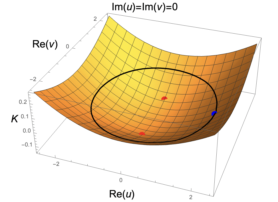
(a) $K$ plotted in the ${\rm Re\,}u$-${\rm Re\,}v$ plane, with ${\rm Im\,}u={\rm Im\,}v=0$, evaluated on a grid with spacing $\delta\text{Re}u=\delta\text{Re}v=0.25$. This slice includes the two Argyres-Douglas points, indicated by the red dots, and one of the multi-monopole points, indicated by the blue dot.

(b) $K$ plotted in the complex $u$-plane, with $v=0$, evaluated on a grid with spacing $\delta\text{Re}u=\delta\text{Im}u=0.25$. The three multi-monopole points are indicated by blue dots.

Figure 3: The $SU(3)$ Kähler potential, plotted numerically on two-real-dimensional slices of the moduli space, using the method of appendix D.2. The $K=0$ contours are depicted in black.

Using both of these numerical techniques, we have evaluated $K$ and its derivatives on many slices through the four-real-dimensional moduli space, with representative plots appearing in figures 3-5. In all cases we observe that $K$ is apparently convex, with no evidence for an extremum away from the origin of moduli space.

Figure 3 depicts two representative numerical plots of $K(u,v)$ on two-dimensional slices of moduli space. In figure 3(a), $K$ is plotted in the $\text{Re}(u)$ and $\text{Re}(v)$ plane with $\text{Im}(u)=\text{Im}(v)=0$. This slice includes the two Argyres-Douglas points at $v=\pm 1$, and one of the three multi-monopole points on the $K=0$ contour. Figure 3(b) is the $SU(3)$ analogue of figure 1 for $SU(2)$, depicting $K$ in the complex $u$-plane at $v=0$ that includes all three multi-monopole points on the $K=0$ contour. Another slicing is shown in 5(a), which depicts $K$ along rays in the complex $u$-plane for various fixed real values of $v$.

All these plots indicate that $K$ is negative around the $\mathbb{Z}_{6}$-symmetric point $u=v=0$ and goes to positive infinity as $u,v\to\infty$. A visualization of the the $K=0$ hypersurface bounding the region of negative $K$ surrounding the origin is depicted in figure 4. In detail, figure 4(a) depicts the complex $u$-plane as a function of real $v$, and figure 4(b) depicts the complex $v$-plane as a function of real $u$. In these slices, the $K=0$ surface is roughly shaped like a cigar, which caps off at approximately $|v|\sim 2.01$ and $|u|\sim 1.89$. Another view of this boundary is depicted in figure 5(b), which shows an almost-circular section of the $K=0$ surface along a ray in the $u$-direction.

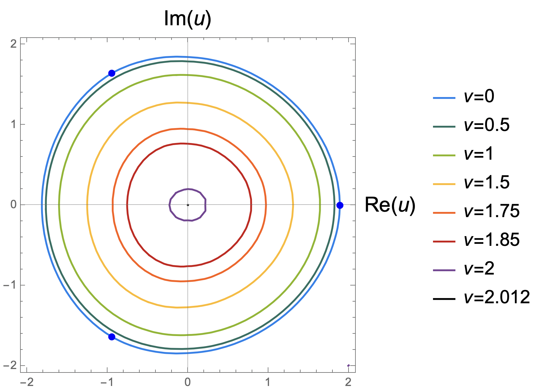
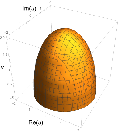
(a) $K=0$ contours in the complex $u$-plane, for real $v\geq 0$. $K$ becomes positive on this slice when $v\gtrsim 2.012$. The blue $v=0$ contour in the left panel includes the three multi-monopole points, indicated by the blue dots. The $K=0$ surface plotted in the right panel is the 3D visualization of the contours plotted in the left panel, and is symmetric under $v\to-v$.

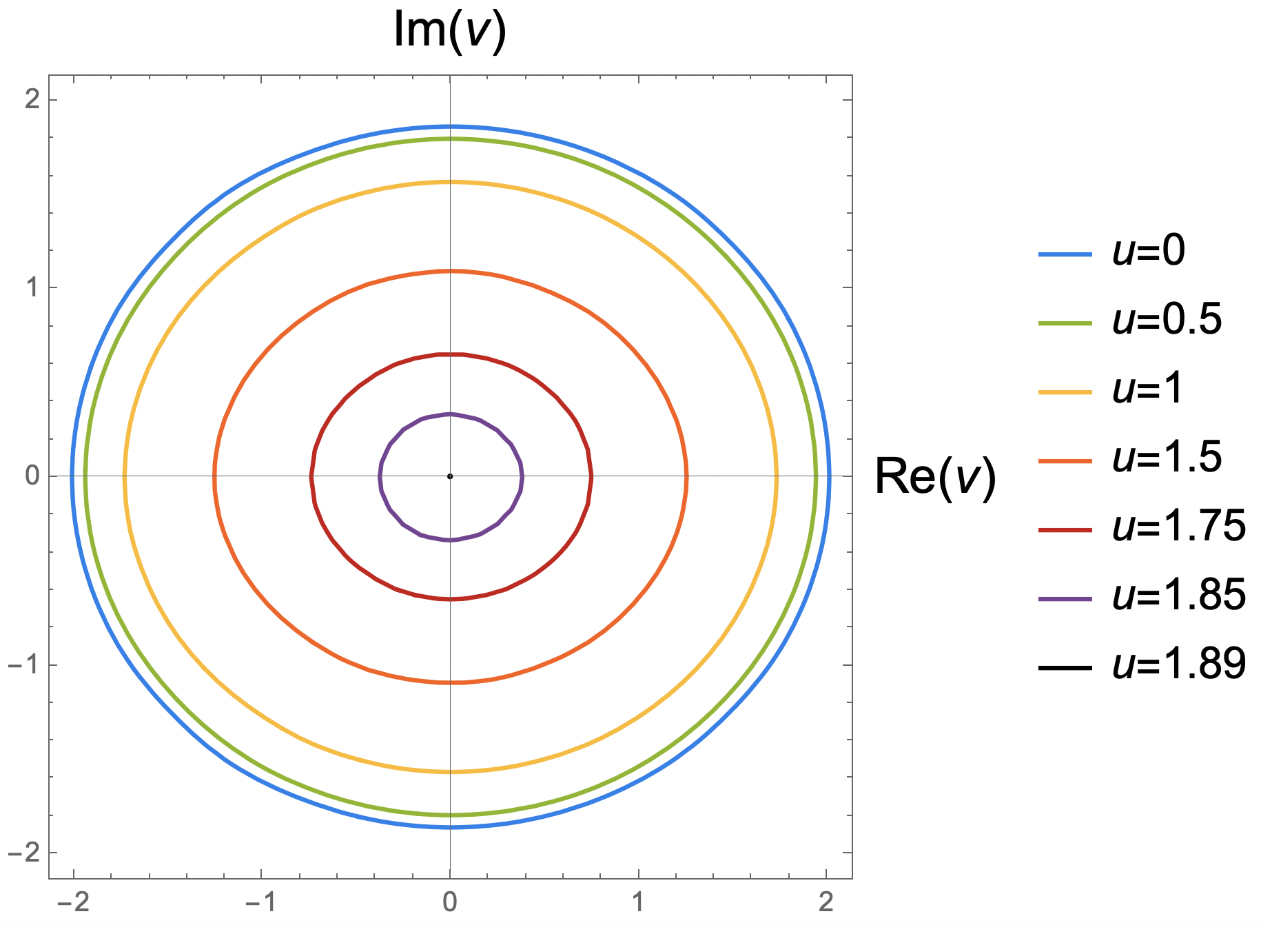
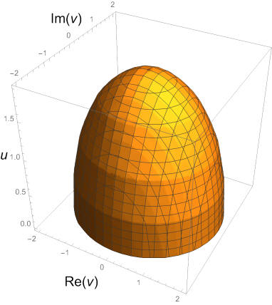
(b) $K=0$ contours in the complex $v$-plane, for real $u\geq 0$. $K$ becomes positive on this slice when $u\gtrsim 1.89$. The $K=0$ surface plotted in the right panel is the 3D visualization of the contours plotted in the left panel.

Figure 4: $K=0$ contours for gauge group $SU(3)$, plotted via the method of appendix D.2.

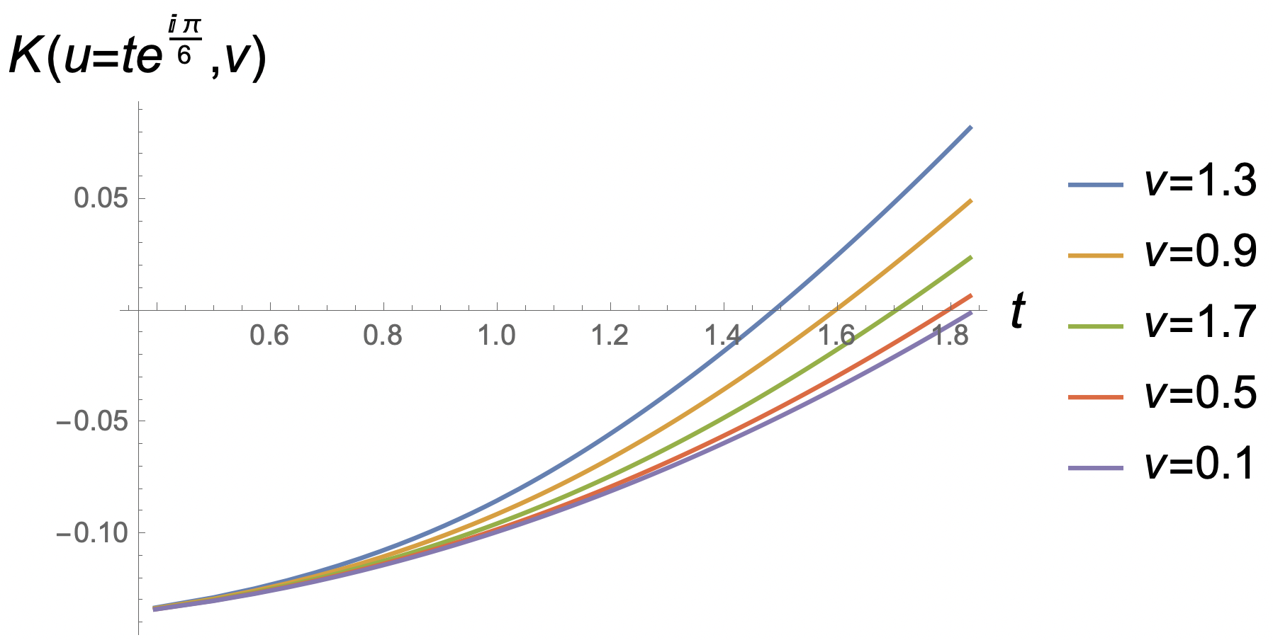
(a) $K$ plotted along rays parameterized by $u=te^{\frac{i\pi}{6}}$, for various real values of $v$. Each ray consists of 100 data points. As $v$ is increased, the region of negative $K$ shrinks.

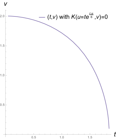
(b) Plot of the (approximately, but not exactly ellipse-shaped) $K=0$ contour in the $(t,v)$ plane, for various real values of $t$ and $v$, with $u=te^{\frac{i\pi}{6}}$. The curve is made up of 36 data points, and is symmetric under $v\to-v$.

Figure 5: Plots of $K$ made using the numerical techniques of appendix D.1.

6 Some Candidate Walls of Marginal Stability

Consider the Coulomb branch of the pure $SU(N)$ gauge theory, where the low-energy gauge group is $U(1)^{N-1}$. In addition to the massless fields on the Coulomb branch, there can be massive particles. These are characterized by their mass $M$, as well as their electric and magnetic charges under the low-energy $U(1)^{N-1}$ gauge group, collectively denoted by a charge vector $\vec{\mu}$,

$$\vec{\mu}=\left(q_{1},\ldots,q_{N-1};g_{1},\ldots,g_{N-1}\right)\in{\mathbb{Z}}^{N}\times{\mathbb{Z}}^{N}~{},$$ (6.1)

with $q_{1},\ldots,q_{N-1}\in{\mathbb{Z}}$ the electric charges and $g_{1},\ldots,g_{N-1}\in{\mathbb{Z}}$ the magnetic ones.

The central charge in the ${\cal N}=2$ supersymmetry algebra is a complex linear function of the charges that depends on the SW periods [1],

$$Z[\vec{\mu}]=\sum_{I=1}^{N-1}\left(q_{I}a_{I}+g_{I}a_{DI}\right)~{}.$$ (6.2)

A single-particle state of mass $M$ and electromagnetic charge vector $\vec{\mu}$ satisfies the following BPS bound [33],

$$M\geq\left|Z[\vec{\mu}]\right|~{}.$$ (6.3)

The particle is a short, or BPS, multiplet of the ${\cal N}=2$ super-Poincaré algebra if and only if this bound is saturated,

$$M_{\text{BPS}}=\left|Z[\vec{\mu}]\right|~{}.$$ (6.4)

Consider two BPS particles with charge vectors $\vec{\mu},\vec{\mu}^{\prime}$ and masses given by (6.4). Henceforth we assume that both charge vectors are non-zero, and that they are not integer multiples of one another. Let us recall that two such particles can in principle form a single-particle bound state (which necessarily has electromagnetic charge vector $\vec{\mu}+\vec{\mu}^{\prime}$) that is also BPS. This happens precisely for threshold bound states (with zero binding energy) whose masses satisfy the following condition,

$$\left|Z[\vec{\mu}+\vec{\mu}^{\prime}]\right|=\left|Z[\vec{\mu}]\right|+\left|Z[\vec{\mu}^{\prime}]\right|~{}.$$ (6.5)

Since $Z$ is a linear function of the charges, this condition saturates the triangle inequality, which is only possible when the complex numbers $Z[\vec{\mu}]$, $Z[\vec{\mu}^{\prime}]$ (and hence also $Z[\vec{\mu}+\vec{\mu}^{\prime}]$) are related by a real proportionality factor,

$$Z[\vec{\mu}^{\prime}]=\zeta\,Z[\vec{\mu}]~{},\qquad\zeta\in{\mathbb{R}}\,.$$ (6.6)

For fixed charge vectors, this real condition carves out a real-codimension-one slice on the Coulomb branch. We refer to this slice as a candidate wall of marginal stability for the BPS particles with charge vectors $\vec{\mu},\vec{\mu}^{\prime}$. Whether or not these particles actually form a bound state upon crossing the wall is a more interesting and delicate question that we do not analyze here.

6.1 Review of Marginal Stability for $SU(2)$

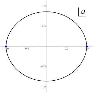
Figure 6: The unique wall of marginal stability in $SU(2)$ gauge theory. The monopole point at $u=1$ and the dyon point at $u=-1$ are indicated as blue dots.

For gauge group $SU(2)$, there is a single pair $\vec{\mu}=(q,g)$ of electromagnetic charges on the Coulomb branch, so that $Z[\vec{\mu}]=qa+ga_{D}$. Given two (non-vanishing and non-parallel) charge vectors $\vec{\mu}=(q,g)$ and $\vec{\mu}^{\prime}=(q^{\prime},g^{\prime})$, the condition (6.6) for a candidate wall of marginal stability then reads

$$(q^{\prime}a+g^{\prime}a_{D})=\zeta(qa+ga_{D})\,,\qquad\zeta\in{\mathbb{R}}\,.$$ (6.7)

Since the charges are all real, this condition can be satisfied if and only if $a$ and $a_{D}$ are themselves related by a real proportionality factor, or equivalently

$${\rm Im\,}\left({a_{D}\over a}\right)=0~{}.$$ (6.8)

This condition defines a (roughly elliptical) curve surrounding the origin $u=0$, which is plotted in figure 6. As shown in [1, 22], inside the wall of marginal stability, there are are precisely two BPS states (together with their antiparticles): the monopole that becomes massless at $u=1$, and the dyon that becomes massless at $u=-1$. Note that these points lie on the wall. The interior of the wall is known as the strong coupling chamber of the moduli space. As the wall is crossed towards the weakly coupled region at infinity, the monopole and the dyon form an infinite tower of BPS bound states comprising the $SU(2)$ W-bosons and the infinite dyon towers that are visible at weak coupling.

Finally, note that the Kähler potential $K\sim{\rm Im\,}a\bar{a}_{D}$ vanishes on the wall of marginal stability, because the condition (6.8) is equivalent to ${\rm Im\,}a\bar{a}_{D}=0$. Thus our notion of strong coupling region, defined as the region where $K<0$, coincides with the standard strong coupling chamber for BPS particles in the case of $SU(2)$ gauge group.

6.2 Some Candidate Walls of Marginal Stability for $SU(3)$

Here we use the expansion of the periods obtained in Corollary 2.4 for $SU(3)$ gauge group to determine candidate walls of marginal stability in special slices of the moduli space, and in a neighborhood that encompasses our strong-coupling region, where $K<0$. It is known that there is an open neighborhood of the origin – termed the strong coupling chamber – in which the BPS spectrum consists of exactly six stable particles (as well as their antiparticles), pairs of which become massless at the three multi-monopole points of $SU(3)$ gauge theory [34, 35, 36]. However, the precise extent of this chamber in moduli space is not known, and our results can serve as a starting point for a more detailed analysis of this question.

6.2.1 The $v=0$ Slice

Figure 7: Candidate wall of marginal stability in the $u$-plane (where $v=0$) for $SU(3)$ gauge group. The three multi-monopole points are indicated as blue dots. In the $u$-plane, the wall coincides with the locus where $K=0$, i.e. it coincides with the outermost contour plotted in figure 4(a).

Inspection of the solution given by Corollary 2.4 shows that $Q_{0,1}=Q_{1,1}=0$ when $v=0$, so that $Q(\xi)=\xi^{4}Q_{0,0}+\xi^{2}Q_{1,0}$. Thus, the periods in the $u$-plane are given by

$$a_{1} = (\rho^{2}-1)Q_{0,0}+(\rho-1)Q_{1,0}\,,$$

$$a_{2} = (\rho^{2}-\rho)Q_{0,0}-(\rho^{2}-\rho)Q_{1,0}\,,$$

$$a_{D1} = (\rho-\rho^{2})Q_{0,0}-(\rho-\rho^{2})Q_{1,0}\,,$$

$$a_{D2} = (\rho^{2}-1)Q_{0,0}+(\rho-1)Q_{1,0}\,,$$ (6.9)

where $\rho=\varepsilon^{2}=e^{2\pi i/3}$. The above expressions for the periods imply the following relations, independently of the values taken by $Q_{0,0}$ and $Q_{1,0}$,

$$a_{2}=-a_{D1}\,,\qquad a_{D2}=a_{1}\,.$$ (6.10)

Let us evaluate the Kähler potential on this slice. Thanks to (6.10), the two pairs of periods contribute equally to $K$, which can now be expressed in terms of $a_{1}$ and $a_{D1}$ only,

$$K={i\over 2\pi}\Big{(}a_{1}\bar{a}_{D1}-\bar{a}_{1}a_{D1}\Big{)}\,.$$ (6.11)

This differs from the Kähler potential for $SU(2)$ by an overall factor of $2$.

Now consider two BPS states with (non-vanishing, non-proportional) charge vectors $\vec{\mu}=(q_{1},q_{2};g_{1},g_{2})$ and $\vec{\mu}^{\prime}=(q_{1}^{\prime},q_{2}^{\prime};g_{1}^{\prime},g_{2}^{\prime})$. Thanks to (6.10) their central charges are given by

$$Z[\vec{\mu}] = (q_{1}+g_{2})a_{1}+(g_{1}-q_{2})a_{D1}~{},$$

$$Z[\vec{\mu}^{\prime}] = (q_{1}^{\prime}+g_{2}^{\prime})a_{1}+(g_{1}^{\prime}-q_{2}^{\prime})a_{D1}\,.$$ (6.12)

Requiring these to be related by a real proportionality factor implies that $a_{1}$ and $a_{D1}$ are also thus related. Thus, as a result of the relations (6.10), this case is completely parallel to the case of $SU(2)$ discussed above: there is a candidate wall of marginal stability defined by the curve $\text{Im}(a_{D1}/a_{1})=0$ in the $u$-plane, depicted in figure 7, and the Kähler potential (6.11) vanishes there.

6.2.2 The $u=0$ Slice

General Discussion

Inspection of the solution given by Corollary 2.4 shows that $Q_{1,0}=Q_{1,1}=0$ for $u=0$, so that $Q(\xi)=\xi^{4}Q_{0,0}+\xi Q_{0,1}$. As a result, the periods are given as follows

$$a_{1} = -(2+\rho)Q_{0,0}+\rho Q_{0,1}\,,$$

$$a_{2} = -(1+2\rho)Q_{0,0}-Q_{0,1}\,,$$

$$a_{D1} = +(1+2\rho)Q_{0,0}-Q_{0,1}\,,$$

$$a_{D2} = -(2+\rho)Q_{0,0}-\rho Q_{0,1}\,,$$ (6.13)

where $\rho=e^{2\pi i/3}$. The above expressions for the periods imply the following inter-relations, independently of the values taken by $Q_{0,0}$ and $Q_{0,1}$,

$$a_{2}=-\rho^{2}\,a_{1}\,,\hskip 72.26999pta_{D2}=\rho\,a_{D1}\,.$$ (6.14)

On this slice, the Kähler potential takes the form

$$K={i\over 4\pi}\Big{(}(1-\rho)a_{1}\bar{a}_{D1}-(1-\rho^{2})\bar{a}_{1}a_{D1}\Big{)}={\sqrt{3}\over 2\pi}\Big{(}|Q_{0,1}|^{2}-3|Q_{0,0}|^{2}\Big{)}\,.$$ (6.15)

As before, we consider two BPS states with (non-vanishing, non-proportional) charge vectors $\vec{\mu}=(q_{1},q_{2};g_{1},g_{2})$ and $\vec{\mu}^{\prime}=(q_{1}^{\prime},q_{2}^{\prime};g_{1}^{\prime},g_{2}^{\prime})$. Substituting these charges and the periods (6.2.2) into the central charge formula (6.2), we find

$$Z[\mu] = (m_{1}+m_{2}\rho)Q_{0,0}+(n_{1}+n_{2}\rho)Q_{0,1}\,,$$

$$Z[\mu^{\prime}] = (m_{1}^{\prime}+m_{2}^{\prime}\rho)Q_{0,0}+(n_{1}^{\prime}+n_{2}^{\prime}\rho)Q_{0,1}\,,$$ (6.16)

where,

$$m_{1} =g_{1}-2g_{2}-2q_{1}-q_{2}\,, n_{1} =g_{1}-q_{2}\,,$$

$$m_{2} =2g_{1}-g_{2}-q_{1}-2q_{2}\,, n_{2} =-g_{2}+q_{1}\,,$$

$$m_{1}^{\prime} =g_{1}^{\prime}-2g_{2}^{\prime}-2q_{1}^{\prime}-q_{2}^{\prime}\,, n_{1}^{\prime} =g_{1}^{\prime}-q_{2}^{\prime}\,,$$

$$m_{2}^{\prime} =2g_{1}^{\prime}-g_{2}^{\prime}-q_{1}^{\prime}-2q_{2}^{\prime}\,, n_{2}^{\prime} =-g_{2}^{\prime}+q_{1}^{\prime}\,.$$ (6.17)

Note that since the charge vector $(g_{1},g_{2};q_{1},q_{2})$ is not identically zero, the same is true for $(m_{1},m_{2};n_{1},n_{2})$, and similarly for the primed charges. Thus $Z[\vec{\mu}],Z[\vec{\mu}^{\prime}]\not=0$ for generic $v$.

The condition (6.6) for a candidate wall of marginal stability, namely $Z[\vec{\mu}^{\prime}]=\zeta Z[\vec{\mu}]$ for $\zeta\in{\mathbb{R}}$, may be expressed as follows,

$$\zeta={az+b\over cz+d}\,,\qquad z={Q_{0,1}\over Q_{0,0}}\,,$$ (6.18)

with

$$a =n_{1}^{\prime}+n_{2}^{\prime}\rho\,, b =m_{1}^{\prime}+m_{2}^{\prime}\rho\,,$$

$$c =n_{1}+n_{2}\rho\,, d =m_{1}+m_{2}\rho\,.$$ (6.19)

We now analyze the implications of these equations, recalling from above that $c$ and $d$ are not both equal to zero. Let us distinguish the following cases:

• For the singular case $ad-bc=0$ the numerator $az+b$ is a constant multiple of the denominator $cz+d$ in (6.18). Since $c$ and $d$ cannot vanish simultaneously, it suffices to analyze the cases $c\not=0$ and $d\not=0$, for which we have the relations,

  $$c\not=0:~{}~{}\zeta={a\over c}\,,\hskip 86.72377ptd\not=0:~{}~{}\zeta={b\over d}\,.$$ (6.20)

  Since $a,b,c,d\in{\mathbb{Z}}[\rho]$, the ratios $a/c$ and $b/d$ may be real or complex. If the ratios are not real, then there can be no solution since $\zeta$ must be real. If the ratios are real, then the charges $\vec{\mu}$, $\vec{\mu}^{\prime}$ are proportional to one another, which we assumed was not the case.

• For the regular case where $ad-bc\not=0$, the relation between $z$ and $\zeta$ may be inverted to give $z$ as a function of $\zeta$,

  $$z={Q_{0,1}\over Q_{0,0}}={d\zeta-b\over-c\zeta+a}\,.$$ (6.21)

  For generic electromagnetic charge vectors, the constants $a,b,c,d$ will be complex, and thus $z$, as a function of $\zeta$, will span an arc of a circle in the complex plane whose center is on the imaginary axis. Below, we will see this explicitly in examples.

Candidate Walls for BPS States that are Stable in the Strong-Coupling Chamber

We will now apply the general discussion above to the six BPS particles that are stable in the strong-coupling chamber of the $SU(3)$ gauge theory. As we review in appendix E, in our conventions these particles have the following electromagnetic charge vectors $(q_{1},q_{2};g_{1},g_{2})$,

$$\begin{split}&\vec{\mu}_{01}=(-1,0;-1,0)~{},\\ &\vec{\mu}_{02}=(0,1;0,-1)~{},\\ &\vec{\mu}_{11}=(1,0;-1,-1)~{},\\ &\vec{\mu}_{12}=(-1,1;0,1)~{},\\ &\vec{\mu}_{21}=(0,1;1,1)~{},\\ &\vec{\mu}_{22}=(1,-1;-1,0)~{}.\end{split}$$ (6.22)

Note that the particle pairs with charges $\vec{\mu}_{k1},\vec{\mu}_{k2}$ become massless at the three multi-monopole points (lying in the $v=0$ slice) corresponding to $k=0,1,2$. Combining with (6.2.2), we see that their central charges in the $u=0$ plane take the following form,

$$Z[\vec{\mu}_{01}] ={\tfrac{1}{2}}(3-i\sqrt{3})(Q_{0,0}+Q_{0,1})\,,$$

$$Z[\vec{\mu}_{02}] ={\tfrac{1}{2}}(3-i\sqrt{3})(Q_{0,0}-Q_{0,1})\,,$$

$$Z[\vec{\mu}_{11}] =-i\sqrt{3}(Q_{0,0}-Q_{0,1})\,,$$

$$Z[\vec{\mu}_{12}] =-i\sqrt{3}(Q_{0,0}+Q_{0,1})\,,$$

$$Z[\vec{\mu}_{21}] =-{\tfrac{1}{2}}(3+i\sqrt{3})(Q_{0,0}+Q_{0,1})\,,$$

$$Z[\vec{\mu}_{22}] =-{\tfrac{1}{2}}(3+i\sqrt{3})(Q_{0,0}-Q_{0,1})\,.$$ (6.23)

Note that the two Argyres-Douglas points lie in the $u=0$ plane, at $v=\pm 1$ (see (5.7)). Evaluating (5.2) at these points, we find the following relations between the $Q$-functions,

$$Q_{0,1}\big{|}_{v=\pm 1}=\pm Q_{0,0}\big{|}_{v=\pm 1}\,.$$ (6.24)

We see that the states $\vec{\mu}_{01},\vec{\mu}_{12},\vec{\mu}_{21}$ are massless at the $v=-1$ Argyres-Douglas point, while the remaining three BPS states $\vec{\mu}_{02},\vec{\mu}_{11},\vec{\mu}_{22}$ are massless at $v=+1$.

Using the central charges in (6.2.2), we can form $\left(\begin{smallmatrix}6\\ 2\end{smallmatrix}\right)=15$ different pairwise ratios, of which six are complex constants $\sim\rho,\rho^{2}$ so that the corresponding central charges can never align. In order to express the alignment conditions for the remaining nine pairs, we use the variable $z=Q_{0,1}/Q_{0,0}$. This leads to the following three cases:

1. The central charges pairwise align as $Z[\vec{\mu}_{01}]\sim Z[\vec{\mu}_{02}]$, $Z[\vec{\mu}_{12}]\sim Z[\vec{\mu}_{11}]$, and $Z[\vec{\mu}_{21}]\sim Z[\vec{\mu}_{22}]$ (with $\sim$ indicating real proportionality) if and only if

   $${1+z\over 1-z}=\zeta\in{\mathbb{R}}\quad\Longleftrightarrow\quad z={\zeta-1\over\zeta+1}~{}.$$ (6.25)

   This describes a horizontal straight line in the complex $z$-plane, i.e. $z=Q_{0,1}/Q_{0,0}$ has to be real, and this can only happen when $v$ is real.

2. The central charges pairwise align as $Z[\vec{\mu}_{01}]\sim Z[\vec{\mu}_{22}]$, $Z[\vec{\mu}_{12}]\sim Z[\vec{\mu}_{02}]$, and $Z[\vec{\mu}_{21}]\sim Z[\vec{\mu}_{11}]$ (with $\sim$ again indicating real proportionality) if and only if

   $$\rho{1+z\over 1-z}=\zeta\in{\mathbb{R}}\quad\Longleftrightarrow\quad z={\rho^{2}\zeta-1\over\rho^{2}\zeta+1}~{}.$$ (6.26)

   This describes a segment of the circle $|z+i/\sqrt{3}|^{2}=4/3$.

3. The central charges pairwise align as $Z[\vec{\mu}_{01}]\sim Z[\vec{\mu}_{11}]$, $Z[\vec{\mu}_{12}]\sim Z[\vec{\mu}_{22}]$, and $Z[\vec{\mu}_{21}]\sim Z[\vec{\mu}_{02}]$ if and only if

   $$-\rho^{2}{1+z\over 1-z}=\zeta\in{\mathbb{R}}\quad\Longleftrightarrow\quad z={\rho\zeta+1\over\rho\zeta-1}~{}.$$ (6.27)

   This describes a segment of the circle $|z-i/\sqrt{3}|^{2}=4/3$.

In the left panel of figure 8 we have plotted the circle described by (6.26) in red, and the one described by (6.27) in blue. There we also indicate in black the curve corresponding to the vanishing of the Kähler potential, $K=0$. As may be read off from (6.15), this curve is a circle in the $z$-plane of radius $\sqrt{3}$.

Figure 8: Candidate curves of marginal stability in the $u=0$ slice for $SU(3)$. In the left panel, the curves are circles of radius $\tfrac{2}{\sqrt{3}}$ centered at $\pm\tfrac{i}{\sqrt{3}}$ in the $z$-plane, and plotted in blue and red. In the right panel, the image of the blue circle is shown in blue and cyan, while the image of the red circle is shown in orange and red. In both panels, the Argyres-Douglas points are indicated by bold black dots, while the $K=0$ curve where the Kähler potential vanishes is plotted in black.

In the right panel of figure 8, the curve of vanishing Kähler potential and the candidate curves of marginal stability are plotted in the $v$-plane. The function $z=Q_{0,1}(0,v)/Q_{0,0}(0,v)$ is holomorphic and single-valued away from the Argyres-Douglas branch points. Thus, the map from $z$ to $v$ is conformal away from the branch points and preserves all angles. Comparison of the curves in the left and right panels of figure 8 clearly shows, however, that the angles between the curves are not preserved at the Argyres-Douglas points, as expected. Using (5.2), the precise expression for the map is given by

$$z={Q_{0,1}(0,v)\over Q_{0,0}(0,v)}={8\pi^{3}\,v\over 2^{{2\over 3}}3^{3}\Gamma(\tfrac{2}{3})^{6}}{F(\tfrac{1}{3},\tfrac{1}{3};\tfrac{3}{2};v^{2})\over F(-\tfrac{1}{6},-\tfrac{1}{6};\tfrac{1}{2};v^{2})}\,.$$ (6.28)

The lowest order approximation, where the hypergeometric functions are set to 1, gives the approximation $z\approx 0.93875\,v$ and translates the circle $|z|^{2}=3$ into the circle $|v|^{2}\approx 3.4043$, which provides a reasonable approximation to the curve of vanishing Kähler potential in the $v$-plane. The behavior near the Argyres-Douglas points may be obtained by using the analytic continuation formulas for the hypergeometric functions, which leads to

$$z=v\Big{(}1-0.47310(1-v^{2})^{5\over 6}+{\cal O}(1-v^{2})\Big{)}\,.$$ (6.29)

The points $v=\pm 1$ are clearly mapped to the points $z=\pm 1$, but the map is not conformal at those points, which explains the widening of the angles in the $v$ plane.

6.3 Generalization to the $u_{0}$ Slice for $SU(N)$

The approach adopted above for the $u=0$ slice in $SU(3)$ extends almost verbatim to the 1-complex-dimensional slice $u_{0}\not=0$ and $u_{n}=0$ with $n=1,\ldots,N-2$ for $SU(N)$ gauge group. Recall from Corollary 2.3 that in this case,

$$a_{DI} = Q(\varepsilon^{2I})-Q(\varepsilon^{2I-1})\,,$$

$$a_{I} = \sum_{J=1}^{I}\Big{\{}Q(\varepsilon^{2J-1})-Q(\varepsilon^{2J-2})\Big{\}}\,,$$ (6.30)

where $\varepsilon=e^{2\pi i/2N}$ and the function $Q(\xi)$ for any $\xi^{2N}=1$ is given by,

$$Q(\xi)=\xi Q_{1}+\xi^{N+1}Q_{N+1}\,,$$ (6.31)

where $Q_{1}$ and $Q_{N+1}$ are functions of $u_{0}$ only. Substituting the form of these functions into the periods, we obtain,

$$a_{DI} = \varepsilon^{2I-1}\Big{\{}(\varepsilon-1)Q_{1}+(\varepsilon+1)Q_{N+1}\Big{\}}\,,$$

$$a_{I} = \sum_{J=1}^{I}\varepsilon^{2J-2}\Big{\{}(\varepsilon-1)Q_{1}-(\varepsilon+1)Q_{N+1}\Big{\}}\,.$$ (6.32)

The central charge of a BPS state with electromagnetic charge vector
$\vec{\mu}=(q_{1},\ldots,q_{N-1};g_{1},\ldots,g_{N-1})$ is given by

$$Z[\vec{\mu}]=mQ_{1}+nQ_{N+1}\,,$$ (6.33)

where $m,n\in{\mathbb{Z}}[\varepsilon]$ are given in terms of the charge vector,

$$m = \sum_{I=1}^{N-1}g_{I}\,\varepsilon^{2I-1}(\varepsilon-1)+\sum_{I=1}^{N-1}q_{I}\,\sum_{J=1}^{I}\varepsilon^{2J-2}(\varepsilon-1)\,,$$

$$n = \sum_{I=1}^{N-1}g_{I}\,\varepsilon^{2I-1}(\varepsilon+1)-\sum_{I=1}^{N-1}q_{I}\,\sum_{J=1}^{I}\varepsilon^{2J-2}(\varepsilon+1)\,.$$ (6.34)

Now we simply repeat the argument used to determine candidate curves of marginal stability in the $u=0$ slice for $SU(3)$ gauge group (see section 6.2.2 above). Consider two charge vectors $\vec{\mu},\vec{\mu}^{\prime}$ with corresponding central charges,

$$Z[\vec{\mu}] = mQ_{1}+nQ_{N+1}\,,$$

$$Z[\vec{\mu}^{\prime}] = m^{\prime}Q_{1}+n^{\prime}Q_{N+1}\,.$$ (6.35)

Marginal stability requires $Z[\vec{\mu}^{\prime}]=\zeta Z[\vec{\mu}]$ for $\zeta\in{\mathbb{R}}$, or equivalently

$$\zeta={n^{\prime}z+m^{\prime}\over nz+m}\,,\hskip 65.04256ptz={Q_{N+1}\over Q_{1}}\,.$$ (6.36)

For the singular case $n^{\prime}m-m^{\prime}n=0$ and, say, $m\not=0$, we have $\zeta=m^{\prime}/m$. There are then two possibilities: if $m^{\prime}/m$ is not real, then there are no solutions; while if $m^{\prime}/m=n^{\prime}/n$ are real, then the charge vectors are proportional to one another. For the regular case $n^{\prime}m-m^{\prime}n\not=0$, the relation between $z$ and $\zeta$ may be inverted and we have,

$$z={Q_{N+1}\over Q_{1}}={m\zeta-m^{\prime}\over-n\zeta+n^{\prime}}\,.$$ (6.37)

For generic charge vectors, $z$ traces an arc of a circle in the complex plane.

Appendix A Proof of Theorem 2.1

In this appendix, we shall provide a complete proof of Theorem 2.1.

A.1 Taylor series expansion of $\lambda$

To obtain a Taylor expansion for the periods $a_{I}$ and $a_{DI}$ at the ${\mathbb{Z}}_{2N}$ symmetric curve, we begin by Taylor expanding the Seiberg-Witten differential in the moduli $u_{n}$ by setting,

$$A(x)=x^{N}-U(x)\,,\hskip 65.04256ptU(x)=\sum_{\ell=0}^{N-2}u_{\ell}\,x^{\ell}\,,$$ (A.1)

and expanding in powers of the polynomial $U(x)$,

$$\lambda=\sum_{m,n=0}^{\infty}{\Gamma(m+{1\over 2})\Gamma(n+{1\over 2})\over\Gamma({1\over 2})^{2}\,m!\,n!}{\big{(}Nx^{N}-xU^{\prime}(x)\big{)}\,U(x)^{m+n}\over(x^{N}-1)^{{1\over 2}+m}(x^{N}+1)^{{1\over 2}+n}}\,dx\,.$$ (A.2)

To obtain this formula, it is convenient to derive the expansions arising from the factors $A(x)\pm 1$ separately and then multiply both series together. Furthermore, to arrive at an integrand whose integrals are easily computed, it will be convenient to multiply numerator and denominator by the factor $(x^{N}+1)^{m}(x^{N}-1)^{n}$, so that all contributions have a common denominator in the form of a power of $(x^{2N}-1)$. Changing summation variables from $m,n$ to $m$ and $M=m+n$, the result may be expressed as follows,

$$\lambda=\sum_{M=0}^{\infty}P_{M}(x^{N})\,{\big{(}Nx^{N}-xU^{\prime}(x)\big{)}\,U(x)^{M}\over(x^{2N}-1)^{{1\over 2}+M}}\,dx~{}.$$ (A.3)

Here we have introduced a family of polynomials $P_{M}(z)$, defined by

$$P_{M}(z)=\sum_{m=0}^{M}{\Gamma(m+{1\over 2})\Gamma(M-m+{1\over 2})\over\Gamma({1\over 2})^{2}\,m!\,(M-m)!}(z+1)^{m}(z-1)^{M-m}\,.$$ (A.4)

Alternatively, one may define these polynomials by their generating function,

$$\sum_{M=0}^{\infty}x^{M}P_{M}(z)={1\over\sqrt{(1-xz)^{2}-x^{2}}}\,.$$ (A.5)

The polynomial $P_{M}(z)$ is of degree $M$ in $z$, satisfies the parity relation $P_{M}(-z)=(-)^{M}P_{M}(z)$, and belongs to a class of polynomials that generalizes Jacobi polynomials. Its expansion in powers of $z$ defines the coefficients $p_{M}(\ell)$ as follows,

$$P_{M}(z)=\sum_{m=0}^{M}p_{M}(m)\,z^{m}\,.$$ (A.6)

The parity relation for $P_{M}(z)$ implies that the coefficients $p_{M}(m)$ vanish unless $M$ and $m$ are either both even or both odd, in which case we have the following expression for $p_{M}(m)$ obtained using Mathematica,

$$p_{M}(m)={2^{m-M}\,M!\over m!\,\Gamma({\tfrac{1}{2}}(M-m)+1)^{2}}~{},\qquad 0\leq m\leq M,\quad M\equiv m~{}(\rm{mod}~{}2)\,.$$ (A.7)

We shall also use the multinomial expansion of $U(x)^{M}$ in powers of the moduli,

$$U(x)^{M}=\sum_{\ell_{0},\ldots,\ell_{N-2}=0}^{\infty}\delta\left(M-\sum_{j=0}^{N-2}\ell_{j}\right)\binom{M}{\ell_{0},\ldots,\ell_{N-2}}\,u_{0}^{\ell_{0}}\cdots u_{N-2}^{\ell_{N-2}}\,x^{L}\,,$$ (A.8)

where $L$ and $M$ are related to the exponents $\ell_{j}$ by

$$L=\sum_{j=0}^{N-2}j\ell_{j}\,,\hskip 65.04256ptM=\sum_{j=0}^{N-2}\ell_{j}\,.$$ (A.9)

Putting all together, we obtain the following expansion for the SW differential,

$$\lambda=\sum_{\ell_{0},\ldots,\ell_{N-2}=0}^{\infty}\binom{M}{\ell_{0},\ldots,\ell_{N-2}}\,u_{0}^{\ell_{0}}\cdots u_{N-2}^{\ell_{N-2}}\,\sum_{m=0}^{M}p_{M}(m)\,\lambda_{M}(Nm+L)\,,\quad$$ (A.10)

where $L$ and $M$ are given in terms of the exponents $\ell_{j}$ by the relations of (A.9) and the differential $(1,0)$-form $\lambda_{M}(k)$ is given as follows,

$$\lambda_{M}(k)={(Nx^{N}-xU^{\prime}(x))\,x^{k}\,dx\over(x^{2N}-1)^{{1\over 2}+M}}~{}.$$ (A.11)

To derive the expansion of Theorem 2.1 we need to obtain the period integrals of the differential $\lambda_{M}(k)$ and to carry out the sum over $m$.

A.2 The basic integrals

The period integrals of $\lambda$ may be expressed in terms of those of $\lambda_{M}(k)$ through (A.10), which in turn may be obtained as finite linear combinations of integrals of the type,

$$\int_{0}^{y}{x^{\gamma-1}\,dx\over\left(x^{2N}-1\right)^{{P\over 2}}}=i^{P}\,{y^{\gamma}\over\gamma}\,F\left({P\over 2},{\gamma\over 2N};1+{\gamma\over 2N};y^{2N}\right)\,,$$ (A.12)

for ${\rm Re\,}(\gamma)>0$ and odd integer $P\geq 1$. The branch cut has been chosen so that $\sqrt{x^{2N}-1}=-i\sqrt{1-x^{2N}}$ when $|x|<1$, for which the square root $\sqrt{1-x^{2N}}$ is positive for $x$ real. Actually, in view of (2.12) and (2.13), evaluating the period integrals requires the above integrals only at the points $y=\xi$ where $\xi^{2N}=1$. To obtain these, we choose the integration path to be the straight line from 0 to $\xi$, as illustrated for $N=3$ by the green lines in figure 2. Since the hypergeometric function then has argument 1, it may be simplified using Gauss’s formula,

$$F(a,b;c;1)={\Gamma(c)\Gamma(c-a-b)\over\Gamma(c-a)\Gamma(c-b)}\,,$$ (A.13)

and we obtain,

$$\int^{\xi}_{0}{x^{\gamma-1}\,dx\over\left(x^{2N}-1\right)^{{P\over 2}}}=i^{P}\,{\xi^{\gamma}\over\gamma}\,{\Gamma(1+{\gamma\over 2N})\Gamma(1-{P\over 2})\over\Gamma(1+{\gamma\over 2N}-{P\over 2})}\,.$$ (A.14)

Using the decomposition of the differential $(1,0)$-form $\lambda_{M}(k)$ in terms of the above integrands,

$$\lambda_{M}(k)={Nx^{N+k}\,dx\over(x^{2N}-1)^{{1\over 2}+M}}-\sum_{j=1}^{N-2}ju_{j}{x^{k+j}\,dx\over(x^{2N}-1)^{{1\over 2}+M}}\,,$$ (A.15)

its integral is readily obtained with the help of (A.14),

$${1\over\pi i}\int^{\xi}_{0}\lambda_{M}(k) = {\xi^{k+N+1}\,\Gamma({k+1\over 2N}+{1\over 2})\over 2\Gamma({k+1\over 2N}+1-M)\Gamma(M+{1\over 2})}\,,$$ (A.16)

$$-\sum_{j=1}^{N-2}j\,u_{j}\,{\xi^{k+j+1}\,\Gamma({k+j+1\over 2N})\over 2N\,\Gamma({k+j+1\over 2N}+{1\over 2}-M)\Gamma(M+{1\over 2})}~{},$$

where we used $\Gamma({1\over 2}-M)\Gamma({1\over 2}+M)=\pi(-)^{M}$ for integer $M$ to simplify the result.

The integral of the SW differential from 0 to an arbitrary $2N$-th root of unity $\xi$,

$$Q(\xi)={1\over\pi i}\int^{\xi}_{0}\lambda\,,$$ (A.17)

may then be expressed in terms of the integrals of the differentials $\lambda_{M}(k)$,

$$W_{M}(\xi,L)=M!\sum_{m=0}^{M}p_{M}(m)\,{1\over\pi i}\int^{\xi}_{0}\lambda_{M}(Nm+L)\,,$$ (A.18)

as follows,

$$Q(\xi)=\sum_{\ell_{0},\ldots,\ell_{N-2}=0}^{\infty}{u_{0}^{\ell_{0}}\cdots u_{N-2}^{\ell_{N-2}}\over\ell_{0}!\cdots\ell_{N-2}!}\,W_{M}(\xi,L)\,,$$ (A.19)

where in both formulas $L$ and $M$ are given in terms of the $\ell_{j}$ by (A.9).

A.3 Carrying out the sum over $m$

Substituting the result (A.16) for the integral of $\lambda_{M}(k)$ into the expression for $W_{M}(\xi,L)$ in (A.18), we obtain

$$W_{M}(\xi,L) = {1\over 2}\,\xi^{NM+L+N+1}\sum_{m=0}^{M}{p_{M}(m)\,\Gamma({m\over 2}+{1\over 2}+{L+1\over 2N})\,M!\over\Gamma({m\over 2}+{L+1\over 2N}+1-M)\Gamma(M+{1\over 2})}$$ (A.20)

$$-{1\over 2N}\xi^{NM+L+j+1}\,\sum_{j=1}^{N-2}j\,u_{j}\,\sum_{m=0}^{M}{p_{M}(m)\,\Gamma({m\over 2}+{L+j+1\over 2N})\,M!\over\Gamma({m\over 2}+{L+j+1\over 2N}+{1\over 2}-M)\Gamma(M+{1\over 2})}\,.$$

We have used the fact that $p_{M}(m)$ vanishes unless $M$ and $m$ are both even or both odd to set $\xi^{Nm}=\xi^{NM}$, thereby allowing us to extract this factor from under the summation symbol. Both sums over $m$ are of the following form for an arbitrary $\gamma\in{\mathbb{C}}$,

$$S_{M}(\gamma)=\sum_{m=0}^{M}{p_{M}(m)\,\Gamma({m\over 2}+\gamma)\,M!\over\Gamma({m\over 2}+\gamma+{1\over 2}-M)\Gamma(M+{1\over 2})}\,,$$ (A.21)

in terms of which $W_{M}$ can be expressed as follows,

$$W_{M}(\xi,L) = {1\over 2}\,\xi^{NM+L+N+1}S_{M}(\tfrac{N+L+1}{2N})-{1\over 2N}\,\xi^{NM+L+1}\sum_{j=1}^{N-2}j\,u_{j}\,\xi^{j}S_{M}(\tfrac{L+j+1}{2N})\,.$$ (A.22)

To evaluate the functions $S_{M}(\gamma)$ we need the following lemma:

Lemma A.1

The function $S_{M}(\gamma)$ evaluates to the following expression,

$$S_{M}(\gamma)={2^{M+1-2\gamma}\over\pi^{2}}\Gamma(2\gamma)\Gamma(\tfrac{M+1}{2}-\gamma)^{2}\sin^{2}\big{(}\pi(\tfrac{M+1}{2}-\gamma)\big{)}~{},$$ (A.23)

for integer $M\geq 0$.

The formula was obtained by induction from the form of $S_{M}(\gamma)$ for low values of $M$, and then verified using Maple for all values of $M$ up to 200. It may be proven analytically by appealing to the hypergeometric function ${}_{3}F_{2}$ as follows: using the explicit expression for $p_{M}(m)$ given in (A.7), the sum over $m$ in $S_{M}(\gamma)$ may be carried out to obtain

$$S_{M}(\gamma)={2^{M+2\sigma}\Gamma(\tfrac{M}{2}+{\tfrac{1}{2}}+\sigma)^{2}\Gamma(\gamma+\sigma)\over\pi\Gamma(M+{\tfrac{1}{2}})\Gamma({\tfrac{1}{2}}+\sigma-M+\gamma)}\,{}_{3}F_{2}\left(\begin{matrix}\sigma-\tfrac{M}{2},\sigma-\tfrac{M}{2},\gamma+\sigma\cr{\tfrac{1}{2}}+2\sigma,{\tfrac{1}{2}}+\sigma-M+\gamma\cr\end{matrix};1\right)\,,$$ (A.24)

where $\sigma=\tfrac{M}{2}-\left[\tfrac{M}{2}\right]$ takes the value $0$ when $M$ is even and ${\tfrac{1}{2}}$ when $M$ is odd. Next, we use the analogue of Gauss’s formula for ${}_{3}F_{2}$,

$${}_{3}F_{2}\left(\begin{matrix}a,b,-n\cr c,1+a+b-c-n\cr\end{matrix};1\right)={\Gamma(c-a+n)\Gamma(c-b+n)\Gamma(c)\Gamma(c-a-b)\over\Gamma(c-a)\Gamma(c-b)\Gamma(c+n)\Gamma(c-a-b+n)}\,,$$ (A.25)

with $a=\sigma-\tfrac{M}{2}$, $b=\gamma+\sigma$, $c={\tfrac{1}{2}}+2\sigma$, and $n=\tfrac{M}{2}-\sigma$. After some simplifications, this expression combines to give the formula of Lemma A.1 and completes its proof.

Substituting Lemma A.1 into (A.22), we find the following formula for $W_{M}(\xi,L)$,

$$W_{M}(\xi,L) = {2^{M-(L+1)/N}\over 2\pi^{2}}\,\xi^{NM+L+N+1}\Gamma(\tfrac{N+L+1}{N})\Gamma(\tfrac{NM-L-1}{2N})^{2}\sin^{2}\big{(}\pi\tfrac{NM-L-1}{2N}\big{)}$$ (A.26)

$$-{2^{M-(L+1)/N}\over\pi^{2}N}\sum_{j=1}^{N-2}j\,u_{j}\,\xi^{NM+j+L+1}\,2^{-\tfrac{j}{N}}\Gamma(\tfrac{j+L+1}{N})\Gamma(\tfrac{NM+N-j-L-1}{2N})^{2}$$

$$\hskip 108.405pt\times\sin^{2}\big{(}\pi\tfrac{NM+N-j-L-1}{2N}\big{)}\,.$$

A.4 Final simplification

We now substitute the formula for $W_{M}(\xi,L)$ in (A.26) above into the expression for $Q(\xi)$ in (A.19) to obtain

$$Q(\xi) = \sum_{\ell_{0},\ldots,\ell_{N-2}=0}^{\infty}{u_{0}^{\ell_{0}}\cdots u_{N-2}^{\ell_{N-2}}\over\ell_{0}!\,\cdots\ell_{N-2}!}{2^{M-(L+1)/N}\over 2\pi^{2}}\,\xi^{NM+L+N+1}\Gamma(\tfrac{N+L+1}{N})\Gamma(\tfrac{NM-L-1}{2N})^{2}\sin^{2}\big{(}\pi\tfrac{NM-L-1}{2N}\big{)}$$ (A.27)

$$-\sum_{\ell_{0},\ldots,\ell_{N-2}=0}^{\infty}{u_{0}^{\ell_{0}}\cdots u_{N-2}^{\ell_{N-2}}\over\ell_{0}!\,\cdots\ell_{N-2}!}{2^{M-(L+1)/N}\over\pi^{2}N}\sum_{j=1}^{N-2}{j\,u_{j}\,\xi^{NM+j+L+1}\over 2^{\tfrac{j}{N}}}\Gamma(\tfrac{j+L+1}{N})$$

$$\hskip 72.26999pt\times\,\Gamma(\tfrac{NM+N-j-L-1}{2N})^{2}\sin^{2}\big{(}\pi\tfrac{NM+N-j-L-1}{2N}\big{)}\,,$$

where on both lines we use the expressions for $L$ and $M$ given in (A.9). In the sum over $j$ on the second and third lines, we combine the lone factor of $u_{j}$ with the monomial $u^{\ell_{j}}\to u_{j}^{\ell_{j}+1}$ and change variables $\ell_{j}+1\to\ell_{j}$. The net effect is to bring out a factor of $\ell_{j}$ and to decrease the values of $M$ and $\ell$ as follows, $M\to M-1$ and $L\to L-j$. Carrying out these three changes at once, and factorizing common parts, gives

$$Q(\xi) = \sum_{\ell_{0},\ldots,\ell_{N-2}=0}^{\infty}{u_{0}^{\ell_{0}}\cdots u_{N-2}^{\ell_{N-2}}\over\ell_{0}!\,\cdots\ell_{N-2}!}{2^{M-(L+1)/N}\over 2\pi^{2}}\,\xi^{NM+L+N+1}\Gamma(\tfrac{NM-L-1}{2N})^{2}$$ (A.28)

$$\qquad\times\sin^{2}\big{(}\pi\tfrac{NM-L-1}{2N}\big{)}\left[\Gamma(1+\tfrac{L+1}{N})-\Gamma(\tfrac{L+1}{N})\sum_{j=0}^{N-2}{j\,\ell_{j}\over N}\right]\,.$$

The expression inside the brackets simplifies to $\Gamma(\tfrac{L+1}{N})/N$, which leads to our final result,

$$Q(\xi) = \sum_{\ell_{0},\ldots,\ell_{N-2}=0}^{\infty}{u_{0}^{\ell_{0}}\cdots u_{N-2}^{\ell_{N-2}}\over\ell_{0}!\,\cdots\ell_{N-2}!}{2^{M-(L+1)/N}\over 2\pi^{2}N}\,\xi^{NM+L+N+1}$$

$$\hskip 57.81621pt\times\Gamma(\tfrac{L+1}{N})\Gamma(\tfrac{NM-L-1}{2N})^{2}\sin^{2}\big{(}\pi\tfrac{NM-L-1}{2N}\big{)}\,.$$

This expression may be recast in the form of Theorem 2.1, thereby completing its proof.

Appendix B The $SU(3)$ Solution in Terms of Appell Functions

In this appendix, we prove Corollary 2.4 and thereby show that the results obtained in Theorem 2.1 for arbitrary $N$ reproduce the solution in terms of Appell functions obtained in [5].

The starting point for the proof is the expression for $Q(\xi)$ for the case $N=3$. We shall use the simplified notation $v=u_{0}$ and $u=u_{1}$, and express the sum in terms of $\ell=\ell_{0}$ and $k=\ell_{1}$ so that $M=k+\ell$ and $L=k$. In terms of these variables, the result of Theorem 2.1 reduces to the following expression for $Q(\xi)$,

$$Q(\xi)=\sum_{k,\ell=0}^{\infty}{2^{(3\ell+2k-1)/3}\over 6\pi^{2}\,k!\,\ell!}\,\xi^{3\ell+4k+4}\,u^{k}\,v^{\ell}\,\Gamma(\tfrac{k+1}{3})\Gamma(\tfrac{3\ell+2k-1}{6})^{2}\sin^{2}\big{(}\pi\tfrac{3\ell+2k-1}{6}\big{)}\,.$$ (B.1)

To decompose the function $Q(\xi)$ into powers of $\xi$, we decompose the summation variables $k$ and $\ell$ modulo 3 and 2 respectively,

$$k =3m+\mu m \geq 0 \mu =0,1,2$$

$$\ell =2n+\nu n \geq 0 \nu =0,1$$ (B.2)

so that the $\xi$-dependence of $Q(\xi)$ is contained entirely in $\mu,\nu$ and independent of $m,n$. The function $Q(\xi)$ then decomposes as follows,

$$Q(\xi) = \sum_{\mu=0,1,2}\,\sum_{\nu=0,1}\xi^{4\mu+3\nu+4}\,Q_{\mu,\nu}$$ (B.3)

$$= \xi^{4}Q_{0,0}+\xi^{2}Q_{1,0}+\xi^{0}Q_{2,0}+\xi^{1}Q_{0,1}+\xi^{5}Q_{1,1}+\xi^{3}Q_{2,1}\,,$$

where the coefficient functions are given by,

$$Q_{\mu,\nu} = {1\over 6\pi^{2}}\sin^{2}\big{(}\pi\tfrac{3\nu+2\mu-1}{6}\big{)}\sum_{m,n=0}^{\infty}{2^{2m+2n+\nu+(2\mu-1)/3}\over(3m+\mu)!\,(2n+\nu)!}\,u^{3m+\mu}\,v^{2n+\nu}$$ (B.4)

$$\hskip 86.72377pt\times\Gamma(m+\tfrac{\mu+1}{3})\Gamma(m+n+\tfrac{3\nu+2\mu-1}{6})^{2}\,.$$

Using the duplication and triplication formulas for the factorials in the denominators,

$$\Gamma(2n+\nu+1) = {2^{2n+\nu}\over\sqrt{\pi}}\Gamma(n+\tfrac{\nu}{2}+{\tfrac{1}{2}})\Gamma(n+\tfrac{\nu}{2}+1)\,,$$

$$\Gamma(3m+\mu+1) = {3^{3m+\mu+{\tfrac{1}{2}}}\over 2\pi}\Gamma(m+\tfrac{\mu}{3}+\tfrac{1}{3})\Gamma(m+\tfrac{\mu}{3}+\tfrac{2}{3})\Gamma(m+\tfrac{\mu}{3}+1)\,,$$ (B.5)

we obtain,

$$Q_{\mu,\nu} = {2^{-1/3}\over 3\sqrt{3\pi}}\sum_{m,n=0}^{\infty}{\sin^{2}\big{(}\pi\tfrac{3\nu+2\mu-1}{6}\big{)}\,\Gamma(m+n+\tfrac{3\nu+2\mu-1}{6})^{2}\,\left({4u^{3}\over 27}\right)^{m+{\mu\over 3}}\,v^{2n+\nu}\over\Gamma(n+\tfrac{\nu}{2}+{\tfrac{1}{2}})\Gamma(n+\tfrac{\nu}{2}+1)\,\Gamma(m+\tfrac{\mu}{3}+\tfrac{2}{3})\Gamma(m+\tfrac{\mu}{3}+1)}\,.$$ (B.6)

Of the six inequivalent representations of ${\mathbb{Z}}_{6}$, $Q_{2,0}$ multiplies the trivial representation of ${\mathbb{Z}}_{6}$ and cancels in the differences giving the periods. Also, the sine-factor vanishes identically for $\mu=2$ and $\nu=1$, so that we have

$$Q_{2,1}=0~{}.$$ (B.7)

The remaining four functions correspond to $\mu,\nu=0,1$ and evaluate as follows,

$$Q_{0,0} = {2^{-1/3}\over 12\sqrt{3\pi}}\sum_{m,n=0}^{\infty}{\Gamma(m+n-\tfrac{1}{6})^{2}\,\over\Gamma(m+\tfrac{2}{3})\Gamma(n+{\tfrac{1}{2}})\,m!\,n!}\,\left({4u^{3}\over 27}\right)^{m}\,v^{2n}\,,$$

$$Q_{0,1} = {2^{-1/3}\over 4\sqrt{3\pi}}\,v\sum_{m,n=0}^{\infty}{\Gamma(m+n+\tfrac{1}{3})^{2}\,\over\Gamma(m+\tfrac{2}{3})\Gamma(n+\tfrac{3}{2})\,m!\,n!}\,\left({4u^{3}\over 27}\right)^{m}\,v^{2n}\,,$$

$$Q_{1,0} = {2^{1/3}\over 36\sqrt{3\pi}}\,u\sum_{m,n=0}^{\infty}{\Gamma(m+n+\tfrac{1}{6})^{2}\over\Gamma(m+\tfrac{4}{3})\Gamma(n+{\tfrac{1}{2}})\,m!\,n!}\,\left({4u^{3}\over 27}\right)^{m}\,v^{2n}\,,$$

$$Q_{1,1} = {2^{1/3}\over 12\sqrt{3\pi}}\,uv\sum_{m,n=0}^{\infty}{\Gamma(m+n+\tfrac{2}{3})^{2}\,\over\Gamma(m+\tfrac{4}{3})\Gamma(n+\tfrac{3}{2})\,m!\,n!}\,\left({4u^{3}\over 27}\right)^{m}\,v^{2n}\,.$$ (B.8)

Using the definition of the Appell function $F_{4}$ in the variables $x=4u^{3}/27$ and $y=v^{2}$, we easily convert these expressions into those stated in Corollary 2.4.

Appendix C Aspects of Elliptic Functions and Modular Forms

In this appendix, we provide a brief review of elliptic functions and modular forms as needed here. A standard and useful reference is [30], whose notations we follow.

C.1 Weierstrass Elliptic Functions

Given a lattice in ${\mathbb{C}}$ with periods $2\omega,2\omega^{\prime}$ the Weierstrass $\wp$ function $\wp(\upsilon|2\omega,2\omega^{\prime})$ satisfies the following differential equation,

$$\left({\partial\wp(\upsilon|2\omega,2\omega^{\prime})\over\partial\upsilon}\right)^{2}=4\,\wp(\upsilon|2\omega,2\omega^{\prime})^{3}-g_{2}(2\omega,2\omega^{\prime})\,\wp(\upsilon|2\omega,2\omega^{\prime})-g_{3}(2\omega,2\omega^{\prime})\,,$$ (C.1)

where each of these quantities is given by the following lattice sums,

$$\wp(\upsilon|2\omega,2\omega^{\prime}) = {1\over\upsilon^{2}}+\sum_{(m,n)\not=(0,0)}\left({1\over(\upsilon+2m\omega+2n\omega^{\prime})^{2}}-{1\over(2m\omega+2n\omega^{\prime})^{2}}\right)\,,$$

$$g_{2}(2\omega,2\omega^{\prime}) = 60\sum_{{m,n}\not=(0,0)}{1\over(2m\omega+2n\omega^{\prime})^{4}}\,,$$

$$g_{3}(2\omega,2\omega^{\prime}) = 140\sum_{{m,n}\not=(0,0)}{1\over(2m\omega+2n\omega^{\prime})^{6}}\,.$$ (C.2)

It will be convenient to use canonical normalizations instead in which the periods are normalized to $1,\tau=\omega^{\prime}/\omega$, and the argument is normalized accordingly to $z=\upsilon/2\omega$. The relation between these two normalizations amounts to a scaling factor by powers of the period $2\omega$ (the functions with both normalizations are denoted by the same symbol),

$$(2\omega)^{-2}\,\wp(z|\tau) = \wp(\upsilon|2\omega,2\omega^{\prime})\,,$$

$$(2\omega)^{-4}\,g_{2}(\tau) = g_{2}(2\omega,2\omega^{\prime})\,,$$

$$(2\omega)^{-6}\,g_{3}(\tau) = \,g_{3}(2\omega,2\omega^{\prime})\,,$$ (C.3)

or equivalently $g_{2}(\tau)=g_{2}(1,\tau)$ and $g_{3}(\tau)=g_{3}(1,\tau)$. In the sequel, the argument $\tau$ will not be exhibited if its dependence is clear from the context. The differential equation for the Weierstrass function is homogeneous under this scaling, and the canonical Weierstrass function $\wp(z)$ satisfies,

$$\wp^{\prime}(z)^{2}=4\,\wp(z)^{3}-g_{2}\wp(z)-g_{3}\,.$$ (C.4)

Henceforth, we shall use this canonical form which is the derivative of the Weierstrass $\zeta(z)$ function (not to be confused with the Riemann $\zeta$-function which will not enter here),

$$\wp(z)=-\zeta^{\prime}(z)\,,\qquad\zeta(-z)=-\zeta(z)\,.$$ (C.5)

The $\zeta(z)$ function has the following monodromy relations,

$$\zeta(z+1)-\zeta(z) = 4\omega\eta\,,\hskip 65.04256pt2\omega\,\eta=\zeta(\tfrac{1}{2})\,,$$

$$\zeta(z+\tau)-\zeta(z) = 4\omega\eta^{\prime}\,,\hskip 65.04256pt2\omega\,\eta^{\prime}=\zeta(\tfrac{\tau}{2})\,.$$ (C.6)

Note that $\zeta(\tfrac{1}{2})$ and $\zeta(\tfrac{\tau}{2})$ are functions of $\tau$ only but, because of the extra factor of $\omega$ in their definition, the parameters $\eta$ and $\eta^{\prime}$ depend on both $\omega$ and $\tau$. The relations are readily established by using the fact that $\zeta(-z)=\zeta(z)$ and setting $z$ equal to $-\tfrac{1}{2}$ and $-\tfrac{\tau}{2}$, respectively. The periods $2\omega$ and $2\omega^{\prime}$ and the parameters $\eta$ and $\eta^{\prime}$ satisfy the following relation,

$$2\eta\,\omega^{\prime}-2\eta^{\prime}\omega=\tau\zeta(\tfrac{1}{2})-\zeta(\tfrac{\tau}{2}) = i\pi\,.$$ (C.7)

One may use this relation to obtain $\eta^{\prime}$ and $\zeta(\tfrac{\tau}{2})$ in terms of the other data. A useful formula for $\zeta(\tfrac{1}{2})$ and thus $\eta$ in terms of the discriminant $\Delta=g_{2}^{3}-27g_{3}^{2}$ is as follows,

$$\zeta(\tfrac{1}{2})=-{i\pi\over 12}\,\partial_{\tau}\ln\Delta={\pi^{2}\over 6}E_{2}(\tau)\,.$$ (C.8)

The combinations $g_{2},g_{3}$ and $\Delta$ are holomorphic modular forms.

C.2 Modular Transformations and Modular Forms

Modular transformations form the group $SL(2,{\mathbb{Z}})$ and act on $\tau$ by Möbius transformations,

$$\tau\to\tilde{\tau}={a\tau+b\over c\tau+d}\,,\hskip 65.04256pt\left(\begin{matrix}a&b\cr c&d\cr\end{matrix}\right)\in SL(2,{\mathbb{Z}})\,.$$ (C.9)

They are generated by the transformations $S$ and $T$, under which $S:\tau\to-1/\tau$ and $T:\tau\to\tau+1$, and whose matrix form is as follows,

$$S=\left(\begin{matrix}0&-1\cr 1&0\cr\end{matrix}\right)\,,\hskip 65.04256ptT=\left(\begin{matrix}1&1\cr 0&1\cr\end{matrix}\right)\,.$$ (C.10)

Under an arbitrary modular transformation $\tau\to\tilde{\tau}$, the half-periods $\omega$ and $\omega^{\prime}$ and the parameters $\eta$ and $\eta^{\prime}$ transform linearly,

$$\tilde{\omega}^{\prime} =a\omega^{\prime}+b\omega\,, \tilde{\eta}^{\prime} =a\eta^{\prime}+b\eta\,,$$

$$\tilde{\omega} =c\omega^{\prime}+d\omega\,, \tilde{\eta} =c\eta^{\prime}+d\eta\,,$$ (C.11)

while the combinations $g_{2}$, $g_{3}$, $\Delta=g_{2}^{3}-27g_{3}^{2}$, and $j=1728\,g_{2}^{3}/\Delta$ transform as follows,

$$g_{2}(\tilde{\tau}) =(c\tau+d)^{4}\,g_{2}(\tau)\,, \Delta(\tilde{\tau}) =(c\tau+d)^{12}\,\Delta(\tau)\,,$$

$$g_{3}(\tilde{\tau}) =(c\tau+d)^{6}\,g_{3}(\tau)\,, j(\tilde{\tau}) =j(\tau)\,.$$ (C.12)

The combinations $g_{2},g_{3}$, and $\Delta$ are referred to as holomorphic modular forms of weight $(4,0)$, $(6,0)$, and $(12,0)$ respectively, while $j$ is a meromorphic modular function, since it is invariant under $SL(2,{\mathbb{Z}})$. We note that $\zeta(\tfrac{1}{2})$ and $\zeta(\tfrac{\tau}{2})$ are not modular forms. Indeed, by combining the expression for $E_{2}$ in terms of $\Delta$ with the transformation law for $\Delta$, we obtain,

$$E_{2}(\tilde{\tau})=(c\tau+d)^{2}E_{2}(\tau)+{12\over 2\pi i}c(c\tau+d)\,,$$ (C.13)

and $E_{2}$ is referred to as a quasi-modular form.

The standard fundamental domain for $SL(2,{\mathbb{Z}})$ is given by,

$${\cal F}=\{\tau\in{\mathbb{C}}\hbox{ such that }0<\tau_{2},\,1\leq|\tau|,\,|\tau_{1}|\leq{\tfrac{1}{2}}\}\,.$$ (C.14)

It contains the orbifold points $i$, $\rho=e^{2\pi i/3}$, and $\rho^{\prime}=\rho+1$, which are fixed points under the transformations $S:i\to i$, $ST:\rho\to\rho$ and $TS:\rho^{\prime}\to\rho^{\prime}$. The $j$-function provides a holomorphic bijection from ${\cal F}$ to the Riemann sphere $\hat{\mathbb{C}}$.

Convergent Taylor series expansions in terms of the variable $e^{2\pi i\tau}$ for $\zeta({\tfrac{1}{2}})$, $g_{2}$ and $g_{3}$ with $\tau$ in the standard fundamental domain ${\cal F}$ are given by

$$\zeta({\tfrac{1}{2}}|\tau) ={\pi^{2}\over 6}E_{2}(\tau)\,, E_{2}(\tau) =1-24\sum_{n=1}^{\infty}\sigma_{1}(n)\,e^{2\pi in\tau}\,,$$

$$g_{2}(\tau) ={4\pi^{4}\over 3}E_{4}(\tau)\,, E_{4}(\tau) =1+240\sum_{n=1}^{\infty}\sigma_{3}(n)\,e^{2\pi in\tau}\,,$$

$$g_{3}(\tau) ={8\pi^{6}\over 27}E_{6}(\tau)\,, E_{6}(\tau) =1-504\sum_{n=1}^{\infty}\sigma_{5}(n)\,e^{2\pi in\tau}\,,$$ (C.15)

where $\sigma_{k}(n)=\sum_{d|n}d^{k}$ with $d>0$ are the standard sum-of-divisor functions. The discriminant takes the form,

$$\Delta(\tau)={(2\pi)^{12}\over 1728}\Big{(}E_{4}(\tau)^{3}-E_{6}(\tau)^{2}\Big{)}=(2\pi)^{12}\,e^{2\pi i\tau}\prod_{n=1}^{\infty}(1-e^{2\pi in\tau})^{24}\,.$$ (C.16)

The $j$-function is normalized so that its pole in $q=e^{2\pi i\tau}$ at the cusp has unit residue,

$$j(\tau)=e^{-2\pi i\tau}+744+{\cal O}(e^{2\pi i\tau})\,.$$ (C.17)

C.3 Special Values

In this final subsection, we review the reality conditions for $g_{2},g_{3},\Delta,E_{2}$ and $\zeta(\tfrac{1}{2})$ and $\zeta(\tfrac{\tau}{2})$, and obtain their special values at the orbifold points $i$ and $\rho$ and at the cusp $i\infty$. The modular function $j$, the modular forms $g_{2},g_{3},\Delta$, as well as $E_{2}$ and thus $\zeta({\tfrac{1}{2}})$ are real for $\tau\in i{\mathbb{R}}$ and $\tau\in\pm{\tfrac{1}{2}}+i{\mathbb{R}}$.

At the orbifold points $i,\,\rho$ and at the cusp $i\infty$, the functions $E_{4}(\tau)$, $E_{6}(\tau)$ , $j(\tau)$, $\zeta({\tfrac{1}{2}}|\tau)$ and $\zeta(\tfrac{\tau}{2}|\tau)$ take the following values,

$$E_{2}(i\infty) =1 E_{2}(i) =\tfrac{3}{\pi} E_{2}(\rho) =\tfrac{2\sqrt{3}}{\pi}$$

$$E_{4}(i\infty) =1 E_{4}(i) =48\Gamma(\tfrac{5}{4})^{4}/(\pi^{2}\Gamma(\tfrac{3}{4})^{4}) E_{4}(\rho) =0$$

$$E_{6}(i\infty) =1 E_{6}(i) =0 E_{6}(\rho) =729\Gamma(\tfrac{4}{3})^{6}/(2\pi^{3}\Gamma(\tfrac{5}{6})^{6})$$

$$j(i\infty) =\infty j(i) =1728 j(\rho) =0$$

$$\zeta({\tfrac{1}{2}}|i\infty) =\tfrac{\pi^{2}}{6} \zeta({\tfrac{1}{2}}|i) =\tfrac{\pi}{2} \zeta({\tfrac{1}{2}}|\rho) =\tfrac{\pi}{\sqrt{3}}$$

$$\zeta(\tfrac{\tau}{2}|\tau) \approx\tfrac{\pi^{2}}{6}\tau-i\pi \zeta(\tfrac{i}{2}|i) =-\tfrac{i\pi}{2} \zeta(\tfrac{\rho}{2}|\rho) =-\tfrac{\pi}{2\sqrt{3}}-\tfrac{i\pi}{2}$$ (C.18)

The values for the cusp $\tau=i\infty$ follow from the series expansions of $E_{2},E_{4}$ and $E_{6}$, and the relation between $\zeta({\tfrac{1}{2}})$ and $E_{2}$ and (C.7). The cancellations of $E_{4}(\rho)$ and $E_{6}(i)$ follow from the modular transformations [37]: the relation $Si=i$ implies $E_{6}(Si)=-E_{6}(i)$ so that $E_{6}(i)=0$ and $j(i)=1728$. Similarly, the relation $ST\rho=\rho$ implies $E_{4}(ST\rho)=\rho^{2}E_{4}(\rho)$ so that $E_{4}(\rho)=0$ and $j(\rho)=0$. The values of $E_{4}(i)$ and $E_{6}(\rho)$ may be found on page 7 in [38].

The values of $\zeta(\tfrac{1}{2}|\tau)$ and $\zeta(\tfrac{\tau}{2}|\tau)$ at the fixed points may be obtained from the values of $E_{2}$ at the fixed points combined with the relations (C.7). Applying the modular transformation rule for $E_{2}$ for the values $\tau=\tilde{\tau}=i$ and $\tau=\tilde{\tau}=i$ with the modular transformations $S$ and $ST$ respectively, we find,

$$E_{2}(i)=-E_{2}(i)+{6\over\pi}\,,\hskip 65.04256ptE_{2}(\rho)=\rho E_{2}(\rho)+{6\rho^{2}\over\pi}\,.$$ (C.19)

Solving these equations gives the entries in the first line of (C.3).

Appendix D Numerical Methods for $SU(3)$

In this appendix, we describe two numerical techniques to evaluate the Kähler potential for the case of $SU(3)$ gauge group.

D.1 Numerically Evaluating $F_{4}$

The Appell function $F_{4}(a,b,c_{1},c_{2};x,y)$ may be evaluated by summing its Taylor series at $x=y=0$ in the domain of convergence $\sqrt{|x|}+\sqrt{|y|}<1$. Beyond this domain, the function enjoys an inversion formula, given in (2.29), which allows one to extend the domain to $\sqrt{|x|}+1<\sqrt{|y|}$ and $\sqrt{|y|}+1<\sqrt{|x|}$. Still, the union of all these domains does not cover all of $x,y\in{\mathbb{C}}$, and in particular excludes the domain that is of greatest interest to us when $|x|\sim|y|\sim 1$. Maple sports a preprogrammed function for $F_{4}$, which has difficulties precisely in this physically interesting region as well. To this end, we now present a numerical approach that circumvents these problems. It is based on numerically integrating a first order ODE along a ray $x(t)=tx,y(t)=ty$ for a given point $(x,y)\in{\mathbb{C}}^{2}$ and $t\in[0,1]$. We shall now present the essential components of the method.

D.1.1 Conversion to a First Order System

Following Appell and Kampé de Fériet [39], we transform the system of two second order differential equations for $F_{4}$,

$$x(1-x)\partial_{x}^{2}f-y^{2}\partial_{y}^{2}f-2xy\partial_{x}\partial_{y}f+\big{(}c_{1}-c_{0}x\big{)}\partial_{x}f-c_{0}y\partial_{y}f-abf = 0$$

$$y(1-y)\partial_{y}^{2}f-x^{2}\partial_{x}^{2}f-2xy\partial_{x}\partial_{y}f+\big{(}c_{2}-c_{0}y\big{)}\partial_{y}f-c_{0}x\partial_{x}f-abf = 0$$ (D.1)

with $c_{0}=a+b+1$, into a system of 4 first order differential equations. Clearly, the dimension of the first order system must be 4 since we know that there must be 4 independent solutions (for generic parameters). Using the notation,

$$p ={\partial f\over\partial x}\,, q ={\partial f\over\partial y}\,, s ={\partial^{2}f\over\partial x\,\partial y}\,,$$ (D.2)

the system of first order differential equations is conveniently expressed in terms of matrix-valued differential form notation,

$$d\Phi=(M_{x}dx+M_{y}dy)\Phi\,,$$ (D.3)

where,

$$\Phi=\left(\begin{matrix}f\cr p\cr q\cr s\cr\end{matrix}\right)\,,\hskip 21.68121ptM_{x}=\left(\begin{matrix}0&1&0&0\cr A_{1}&A_{2}&A_{3}&A_{4}\cr 0&0&0&1\cr C_{1}&C_{2}&C_{3}&C_{4}\cr\end{matrix}\right)\,,\hskip 21.68121ptM_{y}=\left(\begin{matrix}0&0&1&0\cr 0&0&0&1\cr B_{1}&B_{2}&B_{3}&B_{4}\cr D_{1}&D_{2}&D_{3}&D_{4}\cr\end{matrix}\right)\,.$$ (D.4)

The rows that involve only 0 and 1 in $M_{x}$ and $M_{y}$ readily result from the definitions of $p,q,s$ in (D.2). The entries $A_{1},\ldots,A_{4}$ and $B_{1},\ldots,B_{4}$ may be obtained by transforming the system of second order equations into an equivalent system in which one equation involves $\partial_{x}p$ but not $\partial_{y}q$ and vice-versa. This system is given as follows,

$$x(1-x-y)\partial_{x}p-2xys+(c_{1}-c_{1}y-c_{0}x)p+(c_{2}-c_{0})yq-abf = 0\,,$$

$$y(1-x-y)\partial_{y}q-2xys+(c_{2}-c_{2}x-c_{0}y)q+(c_{1}-c_{0})xp-abf = 0\,.$$ (D.5)

As a result, we have,

$$A_{1} ={ab\over x(1-x-y)} B_{1} ={ab\over y(1-x-y)}$$

$$A_{2} ={c_{0}x+c_{1}y-c_{1}\over x(1-x-y)} B_{2} ={(c_{0}-c_{1})x\over y(1-x-y)}$$

$$A_{3} ={(c_{0}-c_{2})y\over x(1-x-y)} B_{3} ={c_{2}x+c_{0}y-c_{2}\over y(1-x-y)}$$

$$A_{4} ={2y\over 1-x-y} B_{4} ={2x\over 1-x-y}$$ (D.6)

To obtain the entries $C_{1},\ldots,C_{4}$ and $D_{1},\ldots,D_{4}$ we begin by taking the $\partial_{y}$ derivative of the first equation in (D.1.1) and the $\partial_{x}$ derivative of the second equation. Taking linear combinations that produce one equation involving only $\partial_{x}s$ and another involving only $\partial_{y}s$ and eliminating the derivatives $\partial_{x}p$ and $\partial_{y}q$ using (D.1.1), one obtains,

$$C_{i}={{\cal C}_{i}\over x(1-x-y)N}\,,\hskip 36.135ptD_{i}={{\cal D}_{i}\over y(1-x-y)N}\,,$$ (D.7)

where $N=(1-x-y)^{2}-4xy$. The coefficients ${\cal C}_{i}$ are given by,

$${\cal C}_{1} = ab(c_{0}-2c_{1}+c_{2}+1)x+ab(c_{0}-c_{2}+1)(1-y)\,,$$

$${\cal C}_{2} = (-2ab+c_{0}^{2}-c_{0}c_{1}+c_{0}c_{2}-c_{1}c_{2}-c_{0}+c_{1})x^{2}$$

$$+(-2ab-c_{0}^{2}+3c_{0}c_{1}+c_{0}c_{2}-2c_{1}^{2}-c_{1}c_{2}-3c_{0}+3c_{1})xy$$

$$+(2ab+c_{0}^{2}-3c_{0}c_{1}-c_{0}c_{2}+2c_{1}^{2}+c_{1}c_{2}+3c_{0}-3c_{1})x\,,$$

$${\cal C}_{3} = (ab-c_{0}c_{2}+c_{2}^{2}+c_{0}-c_{2})(1-x)^{2}+(ab-c_{0}^{2}+c_{0}c_{2})y^{2}$$

$$+(2ab+c_{0}^{2}-2c_{0}c_{1}-2c_{0}c_{2}+2c_{1}c_{2}+c_{2}^{2}+3c_{0}-3c_{2})xy$$

$$+(-2ab+c_{0}^{2}-c_{2}^{2}-c_{0}+c_{2})y\,,$$

$${\cal C}_{4} = (c_{0}-2c_{2}+2)x^{3}+c_{1}y^{3}+(2c_{0}-3c_{1}+2)x^{2}y+(-3c_{0}+2c_{1}+2c_{2}-4)xy^{2}$$ (D.8)

$$+(-2c_{0}-c_{1}+4c_{2}-4)x^{2}-3c_{1}y^{2}+(2c_{0}-4c_{1}+2)xy$$

$$+(c_{0}+2c_{1}-2c_{2}+2)x+3c_{1}y-c_{1}\,,$$

and the coefficients ${\cal D}_{i}$ are given by,

$${\cal D}_{1} = ab(c_{0}-c_{1}+1)(1-x)+ab(c_{0}+c_{1}-2c_{2}+1)y\,,$$

$${\cal D}_{2} = (ab-c_{0}^{2}+c_{0}c_{1})x^{2}+(ab-c_{0}c_{1}+c_{1}^{2}+c_{0}-c_{1})(1-y)^{2}$$

$$+(2ab+c_{0}^{2}-2c_{0}c_{1}-2c_{0}c_{2}+c_{1}^{2}+2c_{1}c_{2}+3c_{0}-3c_{1})xy$$

$$+(-2ab+c_{0}^{2}-c_{1}^{2}-c_{0}+c_{1})x\,,$$

$${\cal D}_{3} = (-2ab+c_{0}^{2}+c_{0}c_{1}-c_{0}c_{2}-c_{1}c_{2}-c_{0}+c_{2})y^{2}$$

$$+(-2ab-c_{0}^{2}+c_{0}c_{1}+3c_{0}c_{2}-c_{1}c_{2}-2c_{2}^{2}-3c_{0}+3c_{2})xy$$

$$+(2ab+c_{0}^{2}-c_{0}c_{1}-3c_{0}c_{2}+c_{1}c_{2}+2c_{2}^{2}+3c_{0}-3c_{2})y\,,$$

$${\cal D}_{4} = c_{2}x^{3}+(c_{0}-2c_{1}+2)y^{3}+(-3c_{0}+2c_{1}+2c_{2}-4)x^{2}y+(2c_{0}-3c_{2}+2)xy^{2}$$ (D.9)

$$-3c_{2}x^{2}+(-2c_{0}+4c_{1}-c_{2}-4)y^{2}+(2c_{0}-4c_{2}+2)xy$$

$$+3c_{2}x+(c_{0}-2c_{1}+2c_{2}+2)y-c_{2}\,.$$

Swapping $x\leftrightarrow y$ and simultaneously $c_{1}\leftrightarrow c_{2}$, we verify $(A_{1},A_{2},A_{3},A_{4})\leftrightarrow(B_{1},B_{3},B_{2},B_{4})$ and $({\cal C}_{1},{\cal C}_{2},{\cal C}_{3},{\cal C}_{4})\leftrightarrow({\cal D}_{1},{\cal D}_{3},{\cal D}_{2},{\cal D}_{4})$.

D.1.2 Solution on a Ray via ODE

Fix a point $(x,y)\in{\mathbb{C}}^{2}$ and parametrize a ray from the ${\mathbb{Z}}_{6}$ symmetric point to $(x,y)$ by

$$x(t) =t\alpha^{2}\,, x =\alpha^{2}\,,$$

$$y(t) =t\beta^{2}\,, y =\beta^{2}\,.$$ (D.10)

In terms of this parametrization, the denominators $(1-x-y)$ and $N$ have simple zeros,

$$1-x(t)-y(t) = 1-t(\alpha^{2}+\beta^{2})\,,$$

$$N(x(t),y(t)) = \big{(}1-t(\alpha-\beta)^{2}\big{)}\big{(}1-t(\alpha+\beta)^{2}\big{)}\,.$$ (D.11)

On this ray, the system of first order equations in two variables collapses to a system in just one variable $t$,

$${d\over dt}\Phi=(\alpha^{2}M_{x}+\beta^{2}M_{y})\Phi\,,$$ (D.12)

where $\Phi$, $M_{x}$, and $M_{y}$ are all evaluated at $x(t),y(t)$. The initial values at the ${\mathbb{Z}}_{6}$-symmetric point may be obtained from the Taylor expansion of $F_{4}$ in powers of $x,y$. The integration of this ODE for each one of the $F_{4}$ functions appearing in the $SU(3)$ solution is now standard, and thankfully proves to be numerically fast.

D.2 Numerically Evaluating the Derivatives of $K$

We now describe a method for numerically evaluating the $SU(3)$ Kähler potential by integrating its derivatives with respect to the moduli $u,v$. Our starting point is the expression (4.4) for the derivatives of $K$ as two-dimensional integrals, which we repeat here

$${\partial K\over\partial\bar{u}_{n}}={1\over 8\pi^{3}}\lim_{R\to\infty}\int_{|x|<R}d^{2}x\,{xA^{\prime}(x)\,\bar{x}^{n}\over|A(x)^{2}-1|}\,,$$ (D.13)

and likewise for the complex conjugate derivatives. For $N=3$ the two complex moduli are $u_{1}=u$ and $u_{0}=v$, with $A(x)=x^{3}-ux-v$.

Straightforward numerical integration of (D.13) fails, due to the fact that the integrand has poles at $x_{i}$ satisfying $A(x_{i})^{2}=1$, as well as at infinity (for the $v$-derivative). We proceed by explicitly subtracting the residues of these poles from the integrand, numerically integrating, and then adding back in the subtracted contributions. For instance, $dK/d\bar{u}$ is computed as

$${\partial K\over\partial\bar{u}} ={2i\over 8\pi^{3}}\lim_{\epsilon\to 0}\left[\int_{-\infty}^{\infty}\int_{-\infty}^{\infty}d\text{Re}(x)\,d\text{Im}(x)\,I(x,\epsilon)+\sum_{i}J(x_{i},\epsilon)\right]\,,$$ (D.14)

where $I(x,\epsilon)$ and $J(x_{i},\epsilon)$ are given as,

$$I(x,\epsilon) = {|x|^{2}A^{\prime}(x)\over|A(x)^{2}-1|}-\frac{3x^{2}}{|x|^{4}}e^{-\frac{1}{|x|^{2}}}-\sum_{i}\frac{|x_{i}|^{2}A^{\prime}(x_{i})e^{-\epsilon|x-x_{i}|^{2}}}{2|A^{\prime}(x_{i})||x-x_{i}|}\,,$$

$$J(x_{i},\epsilon) = \frac{x_{i}A^{\prime}(x_{i})}{2|A^{\prime}(x_{i})|}(2\pi)\int_{0}^{\infty}\,dr\,e^{-\epsilon r^{2}}\,.$$ (D.15)

When evaluating these formulas numerically we take $\epsilon$ to be a small number (e.g. $\epsilon=0.01$) whose precise value demonstrably does not affect the results of the integration. The expression (D.14) for $\partial K/\partial\bar{u}$, along with the analogous formulae for $\partial K/\partial\bar{v}$ and their complex conjugates, can then be straightforwardly numerically integrated from an initial point (which we take to be the multi-monopole point with real $u$ for which $K=0$) to a generic point $(u,v)$. In this way, $K$ can be evaluated on a grid of complex $(u,v)$ values.

We have subjected the numerical evaluation method described above to various consistency checks:

• Applying the same method to the case of $SU(2)$ gauge group, we have verified that the resulting $K(u)$ matches the known hypergeometric function representation depicted in figure 1.

• We have verified that on the $u=0$ and $v=0$ slices of moduli space for which the Appell functions reduce to hypergeometric functions, the numeric evaluation of $K(u,v)$ reproduces the correct values. This includes matching to the analytic values of $K$ at the origin (computed in (3.10)) and at the Argyres-Douglas points (computed in (5.27)).

• Within the region of convergence of Maple’s predefined Appell $F_{4}$ function, we have verified for a variety of $(u,v)$ that the numerical evaluation of $K(u,v)$ matches the numerical evaluation of the exact formula of $K$ given in terms of Appell functions.

• We have, in some regimes, checked the two numerical methods described in appendices D.1 and D.2 against each other and found them to match with high precision.

Appendix E The Strong-Coupling Spectrum for $SU(N)$

In this appendix, we enumerate the stable BPS particles in the strong-coupling chamber of four-dimensional $\mathcal{N}=2$ pure supersymmetric gauge theory with gauge group $SU(N)$, though our primary interest is the case $N=3$.

These BPS states were determined, for all $SU(N)$ gauge groups, in [34, 35, 36]. We follow the discussion in [35], where a basis different from ours is used. It is convenient to work at the origin of moduli space, i.e. at the ${\mathbb{Z}}_{2N}$-symmetric point. The left panel of figure 9 shows the branch cut conventions and various cycles used in [35], while the right panel shows our choice of branch cuts and cycles, both for the case of $SU(3)$ gauge group. We see that the branch cuts, as well as the $\hat{\mathfrak{A}}_{I}$ (and hence the ${\mathfrak{A}}_{I}$) cycles and the intersection pairing $\#(\mathfrak{A}_{I},\mathfrak{B}_{J})=\delta_{IJ}$, are the same in both figures. However, the figures differ in the definition of the $\mathfrak{B}_{I}$ cycles.

In order to translate their results into our conventions, we denote their $\mathfrak{B}_{I}$ cycles – referring to the left panel of figure 9 – by $\mathfrak{B}_{I}^{\text{them}}$, while our $\mathfrak{B}_{I}$ cycles – referring to the right panel of figure 9 – are denoted by $\mathfrak{B}_{I}^{\text{us}}$. By examining these figures, we see that the cycles are related as follows,

$$\mathfrak{B}_{1}^{\text{us}}=\mathfrak{B}_{1}^{\text{them}}-\mathfrak{A}_{1}\,,\hskip 65.04256pt\mathfrak{B}_{2}^{\text{us}}=\mathfrak{B}_{2}^{\text{them}}+\mathfrak{A}_{2}\,.$$ (E.1)

Figure 9: The left panel shows the conventions for the $\hat{\mathfrak{A}}_{I}$, $\mathfrak{B}_{I}$, and $\mathfrak{C}_{I}$ cycles that are used in [35]. The right panel shows our conventions for the $\hat{\mathfrak{A}}_{I},\mathfrak{B}_{I}$ cycles. In this figure we have specialized to $N=3$, with $\varepsilon=e^{\frac{2\pi i}{6}}$.

In the conventions of [35], the $N(N-1)$ BPS particles that exist at the origin of $SU(N)$ gauge theory have charge vectors $\vec{\mu}_{kI}$ that correspond to the following cycles $\mu_{kI}$,

$$\mu_{0I}=-\mathfrak{B}_{I}^{\text{them}}\,,\hskip 28.90755pt\mu_{1I}=\mathfrak{C}_{I}\,,\hskip 28.90755pt\mu_{kI}=\mu_{k-1,I-1}+\mu_{k-1,I+1}-\mu_{k-2,I}\,.$$ (E.2)

Here the labels run over $k=2,\ldots,N-1$ and $I=1,\ldots,N-1$, so that we set $\mu_{kI}=0$ for $I<1$ and $I>N-1$. The $\mathfrak{C}_{I}$ cycle is obtained from $\mathfrak{B}^{\text{them}}_{I}$ by a $-\frac{\pi}{N}$ rotation, as indicated in figure 9 for the case $N=3$. It can be expressed in terms of the $\mathfrak{A}_{I}$ and $\mathfrak{B}^{\text{them}}_{I}$ cycles:

$$\mathfrak{C}_{I}=\left\{\begin{array}[]{cc}-\mathfrak{A}_{I-1}+2\mathfrak{A}_{I}-\mathfrak{A}_{I+1}+\mathfrak{B}^{\text{them}}_{I}&I\ \text{even}\\ -\mathfrak{A}_{I-1}+2\mathfrak{A}_{I}-\mathfrak{A}_{I+1}-\mathfrak{B}^{\text{them}}_{I-1}-\mathfrak{B}^{\text{them}}_{I}-\mathfrak{B}^{\text{them}}_{I+1}&I\ \text{odd}\end{array}\right.\,.$$ (E.5)

The tower of $N-1$ mutually local dyons that become massless at the $k$’th multi-monopole point corresponds to the set of $\mu_{kI}$ cycles, with $I=1,\cdots,N-1$.

$\mu_{kI}$	Cycles	$(\vec{q};\vec{g})^{\text{them}}$	$(\vec{q};\vec{g})^{\text{us}}$
$\mu_{01}$	$-\mathfrak{B}_{1}^{\text{them}}$	$(0,0;-1,0)$	$(-1,0;-1,0)$
$\mu_{02}$	$-\mathfrak{B}^{\text{them}}_{2}$	$(0,0;0,-1)$	$(0,1;0,-1)$
$\mu_{11}$	$\mathfrak{C}_{1}=2\mathfrak{A}_{1}-\mathfrak{A}_{2}-\mathfrak{B}^{\text{them}}_{1}-\mathfrak{B}^{\text{them}}_{2}$	$(2,-1;-1,-1)$	$(1,0;-1,-1)$
$\mu_{12}$	$\mathfrak{C}_{2}=-\mathfrak{A}_{1}+2\mathfrak{A}_{2}+\mathfrak{B}^{\text{them}}_{2}$	$(-1,2;0,1)$	$(-1,1;0,1)$
$\mu_{21}$	$\mathfrak{C}_{2}+\mathfrak{B}^{\text{them}}_{1}$	$(-1,2;1,1)$	$(0,1;1,1)$
$\mu_{22}$	$\mathfrak{C}_{1}+\mathfrak{B}^{\text{them}}_{2}$	$(2,-1;-1,0)$	$(1,-1;-1,0)$

Table 1: The six stable BPS particles in the strong-coupling chamber of $SU(3)$ gauge theory, together with the corresponding cycles and charges in the conventions of [35], as well as the translation of the charges into our conventions.

Specializing to $N=3$, there are six BPS particles in the strong-coupling chamber, corresponding to cycles $\mu_{kI}$ with $k=0,1,2$ and $I=1,2$. The corresponding charges $\vec{\mu}^{\text{them}}=(\vec{q};\vec{g})^{\text{them}}$ can be read off immediately from the specialization of (E.2) and (E.5) to $N=3$, while the charges $\vec{\mu}^{\text{us}}=(\vec{q};\vec{g})^{\text{us}}$ in our basis can be determined from (E.1),

$$\begin{split}\vec{g}^{\text{us}}&=\vec{g}^{\text{them}}~{},\\ q_{1}^{\text{us}}&=q_{1}^{\text{them}}+g_{1}^{\text{them}}~{},\\ q_{2}^{\text{us}}&=q_{2}^{\text{them}}-g_{2}~{}.\end{split}$$ (E.6)

The results are summarized in table 1. The states in the table are grouped into three pairs $\mu_{kI}$, labeled by $k=0,1,2$, of mutually local dyons, with one pair becoming massless at each of the three multi-monopole points. At each of the two Argyres-Douglas points, one dyon from each pair becomes massless. At the origin of moduli space, all six states are massive and degenerate.

References

- [1] N. Seiberg and E. Witten, “Electric - magnetic duality, monopole condensation, and confinement in N=2 supersymmetric Yang-Mills theory,” Nucl. Phys. B426 (1994) 19–52, arXiv:hep-th/9407087 [hep-th]. [Erratum: Nucl. Phys.B430,485(1994)].
- [2] N. Seiberg and E. Witten, “Monopoles, duality and chiral symmetry breaking in n = 2 supersymmetric QCD,” Nuclear Physics B 431 no. 3, (Dec, 1994) 484–550. https://doi.org/10.1016%2F0550-3213%2894%2990214-3.
- [3] A. Klemm, W. Lerche, S. Yankielowicz, and S. Theisen, “Simple singularities and N=2 supersymmetric Yang-Mills theory,” Phys. Lett. B344 (1995) 169–175, arXiv:hep-th/9411048 [hep-th].
- [4] P. C. Argyres and A. E. Faraggi, “The vacuum structure and spectrum of N=2 supersymmetric SU(n) gauge theory,” Phys. Rev. Lett. 74 (1995) 3931–3934, arXiv:hep-th/9411057 [hep-th].
- [5] A. Klemm, W. Lerche, and S. Theisen, “Nonperturbative effective actions of N=2 supersymmetric gauge theories,” Int. J. Mod. Phys. A 11 (1996) 1929–1974, arXiv:hep-th/9505150.
- [6] E. D’Hoker, I. M. Krichever, and D. H. Phong, “The Effective prepotential of N=2 supersymmetric SU(N(c)) gauge theories,” Nucl. Phys. B 489 (1997) 179–210, arXiv:hep-th/9609041.
- [7] E. D’Hoker, I. M. Krichever, and D. H. Phong, “The Renormalization group equation in N=2 supersymmetric gauge theories,” Nucl. Phys. B 494 (1997) 89–104, arXiv:hep-th/9610156.
- [8] E. D’Hoker and D. H. Phong, “Strong coupling expansions of SU(N) Seiberg-Witten theory,” Phys. Lett. B 397 (1997) 94–103, arXiv:hep-th/9701055.
- [9] T. Masuda and H. Suzuki, “Prepotential of N=2 supersymmetric Yang-Mills theories in the weak coupling region,” Int. J. Mod. Phys. A 13 (1998) 1495–1506, arXiv:hep-th/9609065.
- [10] J. D. Edelstein and J. Mas, “Strong coupling expansion and Seiberg-Witten-Whitham equations,” Phys. Lett. B 452 (1999) 69–75, arXiv:hep-th/9901006.
- [11] J. D. Edelstein and J. Mas, “N=2 supersymmetric Yang-Mills theories and Whitham integrable hierarchies,” AIP Conf. Proc. 484 (1999) 195–212, arXiv:hep-th/9902161.
- [12] E. D’Hoker, T. T. Dumitrescu, E. Gerchkovitz, and E. Nardoni, “Revisiting the multi-monopole point of SU(N) = 2 gauge theory in four dimensions,” JHEP 09 (2021) 003, arXiv:2012.11843 [hep-th].
- [13] K. Ito and S.-K. Yang, “Prepotentials in N=2 SU(2) supersymmetric Yang-Mills theory with massless hypermultiplets,” Phys. Lett. B 366 (1996) 165–173, arXiv:hep-th/9507144.
- [14] J. M. Isidro, A. Mukherjee, J. P. Nunes, and H. J. Schnitzer, “A New derivation of the Picard-Fuchs equations for effective N=2 superYang-Mills theories,” Nucl. Phys. B 492 (1997) 647–681, arXiv:hep-th/9609116.
- [15] M. Alishahiha, “On the Picard-Fuchs equations of the SW models,” Phys. Lett. B 398 (1997) 100–103, arXiv:hep-th/9609157.
- [16] C. Córdova and T. T. Dumitrescu, “Candidate Phases for SU(2) Adjoint QCD4 with Two Flavors from Supersymmetric Yang-Mills Theory,” arXiv:1806.09592 [hep-th].
- [17] Z. Komargodski and N. Seiberg, “Comments on Supercurrent Multiplets, Supersymmetric Field Theories and Supergravity,” JHEP 07 (2010) 017, arXiv:1002.2228 [hep-th].
- [18] T. T. Dumitrescu and N. Seiberg, “Supercurrents and Brane Currents in Diverse Dimensions,” JHEP 07 (2011) 095, arXiv:1106.0031 [hep-th].
- [19] E. D’Hoker, T. T. Dumitrescu, E. Gerchkovitz, and E. Nardoni, “to appear,”.
- [20] M. A. Luty and R. Rattazzi, “Soft supersymmetry breaking in deformed moduli spaces, conformal theories, and N=2 Yang-Mills theory,” JHEP 11 (1999) 001, arXiv:hep-th/9908085.
- [21] M. R. Douglas and S. H. Shenker, “Dynamics of SU(N) supersymmetric gauge theory,” Nucl. Phys. B 447 (1995) 271–296, arXiv:hep-th/9503163.
- [22] F. Ferrari and A. Bilal, “The Strong coupling spectrum of the Seiberg-Witten theory,” Nucl. Phys. B 469 (1996) 387–402, arXiv:hep-th/9602082.
- [23] B. J. Taylor, “On the strong coupling spectrum of pure SU(3) Seiberg-Witten theory,” JHEP 08 (2001) 031, arXiv:hep-th/0107016.
- [24] B. J. Taylor, “On the moduli space of SU(3) Seiberg-Witten theory with matter,” JHEP 12 (2002) 040, arXiv:hep-th/0211086.
- [25] D. Galakhov, P. Longhi, T. Mainiero, G. W. Moore, and A. Neitzke, “Wild Wall Crossing and BPS Giants,” JHEP 11 (2013) 046, arXiv:1305.5454 [hep-th].
- [26] P. C. Argyres and M. R. Douglas, “New phenomena in SU(3) supersymmetric gauge theory,” Nucl. Phys. B 448 (1995) 93–126, arXiv:hep-th/9505062.
- [27] L. Alvarez-Gaume and S. F. Hassan, “Introduction to S duality in N=2 supersymmetric gauge theories: A Pedagogical review of the work of Seiberg and Witten,” Fortsch. Phys. 45 (1997) 159–236, arXiv:hep-th/9701069.
- [28] B. Ananthanarayan, S. Friot, S. Ghosh, and A. Hurier, “New analytic continuations for the Appell series from quadratic transformations of the Gauss function,” arXiv:2005.07170 [hep-th].
- [29] H. M. Farkas and I. Kra, Riemann surfaces. Springer.
- [30] A. Erdelyi, ed., Higher Transcendental Functions, vol. II, ch. XIII. Robert E. Krieger Publishing Company, London, 1981.
- [31] Wikipedia, “J-invariant — Wikipedia, the free encyclopedia.” http://en.wikipedia.org/w/index.php?title=J-invariant&oldid=1082234111, 2022. [Online; accessed 05-July-2022].
- [32] E. D’Hoker, M. B. Green, and B. Pioline, “Asymptotics of the genus-two string invariant,” Commun. Num. Theor. Phys. 13 (2019) 351–462, arXiv:1806.02691.
- [33] E. Witten and D. I. Olive, “Supersymmetry Algebras That Include Topological Charges,” Phys. Lett. B 78 (1978) 97–101.
- [34] W. Lerche, “On a boundary CFT description of nonperturbative N=2 Yang-Mills theory,” arXiv:hep-th/0006100.
- [35] M. Alim, S. Cecotti, C. Cordova, S. Espahbodi, A. Rastogi, and C. Vafa, “ quantum field theories and their BPS quivers,” Adv. Theor. Math. Phys. 18 no. 1, (2014) 27–127, arXiv:1112.3984 [hep-th].
- [36] W.-y. Chuang, D.-E. Diaconescu, J. Manschot, G. W. Moore, and Y. Soibelman, “Geometric engineering of (framed) BPS states,” Adv. Theor. Math. Phys. 18 no. 5, (2014) 1063–1231, arXiv:1301.3065 [hep-th].
- [37] T. A. Apostol, Modular Functions and Dirichlet Series in Number Theory. Springer Verlag, 1976.
- [38] F. Diamond and J. Shurman, A first course in modular forms. Springer, 2005.
- [39] P. Appell and J. Kampé de Fériet, Fonctions Hyper-géometriques and Hyper-sphériques - Polynomes d’Hermite. Gauthier-Villars, 1929.