Electron-mediated projective quantum nondemolition measurement on a nuclear spin

Abstract

Projective quantum nondemolition (QND) measurement is important for quantum technologies. Here we propose a method for constructing projective QND measurement on a nuclear spin via the measurement of an axillary electron spin in generic electron-nuclear spin systems coupled through weak hyperfine interaction. The key idea is to apply suitable quantum control on the electron to construct a weak QND measurement on the nuclear spin and then cascade a sequence of such measurements into a projective one. We identify a set of tunable parameters to select the QND observables and control the strength of the weak QND measurement. We also find that the QND measurement can be stabilized against realistic experimental control errors. As a demonstration of our method, we design projective QND measurement on a ¹³C nuclear spin weakly coupled to a nitrogen-vacancy center electron spin in diamond.

I Introduction

Measurement backaction Wiseman and Milburn (2010) is the measurement-induced non-unitary disturbance on the system being measured. To overcome the downgrade of measurement precision caused by the random disturbance, quantum nondemolition (QND) was introduced Braginsky and Vorontsov (1975); Braginskii et al. (1977); Thorne et al. (1978); Unruh (1979); Caves et al. (1980); Braginsky et al. (1980). The key idea is to measure an observable that is conserved during the free evolution, so that its value remains unaffected between successive measurements and sufficient statistics can be build up to improve the signal-to-noise ratio Clerk et al. (2010). QND has been demonstrated experimentally in quantum optics Grangier et al. (1998), microscopic superconducting systems Lupascu et al. (2007) and trapped single electron Peil and Gabrielse (1999).

In hybrid electron-nuclear spin systems, the nuclear spin qubits can be exploited as quantum resources due to their long coherence times Laraoui et al. (2013); Staudacher et al. (2015); Mamin et al. (2013); Wang et al. (2017); Zaiser et al. (2016); Shi et al. (2014, 2015); Du et al. (2009); Pfender et al. (2017); Rosskopf et al. (2017); Schmitt et al. (2017); Glenn et al. (2018); Muhonen et al. (2014); Saeedi et al. (2013); Tyryshkin et al. (2012); Press et al. (2010). Projective QND measurement on the nuclear spin qubits is important for scalable quantum computation Taminiau et al. (2014), quantum sensing Pfender et al. (2017); Rosskopf et al. (2017) and quantum communication Yang et al. (2016). The quantum measurement of the nuclear spin is difficult and is often realized indirectly via measurement of a nearby electron spin Dreau et al. (2013); Neumann et al. (2010), e.g., mapping the population of a nearby nuclear spin onto the electron spin via controlled-NOT gates allows projective QND measurements of the nuclear spin $z$ component $\hat{I}_{z}$ – a conserved observable protected by the external magnetic field Dreau et al. (2013); Neumann et al. (2010). However, remote nuclear spins weakly coupled to the electron (i.e., coupling strength $<1/T_{2}^{\ast}$) can hardly be resolved or manipulated to implement the controlled-NOT gates reliably. Moreover, the transverse components $(I_{x},I_{y})$ of the nuclear spin are not conserved, so their projective QND measurements are nontrivial. Recently, single-shot readout of nuclear a spin-1/2 weakly coupled to an nitrogen-vacancy center electron spin in diamond was demonstrated experimentally by using a series of weak measurements to trap the target nuclear spin and then read out its state repeatedly Liu et al. (2017), but its connection to QND remains unclear.

In this paper, we propose a general method to construct projective QND measurements on non-conserved observables (e.g., the transverse components) of a nuclear spin weakly coupled to an axillary electron spin via hyperfine interaction. The procedure consists of two steps. First, dynamical decoupling control is applied to the electron spin to establish electron-nuclear entanglement, followed by a projective measurement on the electron spin to mediate a single weak measurement on the nuclear spin. Second, we apply a sequence of such weak measurements to the nuclear spin and tune the evolution of the nuclear spin between neighboring measurements to meet the stroboscopic QND condition Braginsky et al. (1978); Thorne et al. (1978); Caves et al. (1980); Braginsky et al. (1980); Jordan and Büttiker (2005); Ruskov et al. (2005); Jordan et al. (2006); Averin et al. (2006); Jordan and Korotkov (2006), so that this sequence of weak QND measurements form a single projective QND measurement on the nuclear spin. We identify a set of tunable parameters for flexible, in situ control of the QND observable and find optimal parameters to stabilize the QND measurements against control errors. This work is relevant to state preparation, quantum sensing, and quantum error correction via projective QND measurements.

The paper is organized as follows. In Sec. II, we construct a single weak measurement on the nuclear spin via measurement of the electron spin. In Sec. III, we use a sequence of weak QND measurements to form a single projective QND measurement and analyze its stability against control errors. In Sec. IV, we illustrate our method in a paradigmatic physical system, i.e., a ¹³C nuclear spin weakly coupled to a nitrogen-vacancy center electron spin in diamond Liu et al. (2017). In Sec. V, we draw the conclusions.

II Electron-mediated measurement on nuclear spin

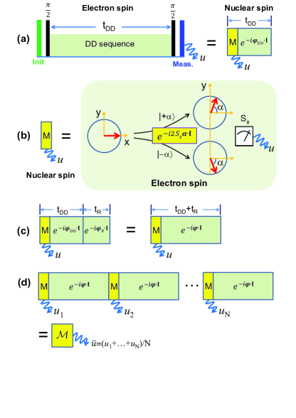
Figure 1: (a) Control sequence on an auxillary electron spin coupled to the target nuclear spin via hyperfine interaction. This mediates an effective measurement (yellow box “M”) on the target nuclear spin followed by a rotation $e^{-i\boldsymbol{\varphi}_{\mathrm{DD}}\cdot\mathbf{\hat{I}}}$. (b) The effective measurement on the nuclear spin originates from the conditional rotation of the electron spin (red arrows) around the $z$ axis by opposite angles for opposite nuclear spin initial states $|\pm\alpha\rangle$ – the two eigenstates of $\boldsymbol{\hat{\alpha}}\cdot\mathbf{\hat{I}}$, and the subsequent projective measurement on the electron spin observable $\hat{S}_{\phi}\equiv\mathbf{\hat{S}}\cdot\mathbf{e}_{\phi}$, where $\mathbf{e}_{\phi}=\mathbf{e}_{x}\cos\phi+\mathbf{e}_{y}\sin\phi$. (c) Immediately after the $\hat{S}_{\phi}$ measurement, we re-initialize the electron spin into $|+\rangle$ and append a waiting time $t_{R}$, during which we flip the electron spin to engineer the nuclear spin evolution $e^{-i\boldsymbol{\varphi}_{R}\cdot\mathbf{\hat{I}}}$. The total evolution of the nuclear spin after the measurement becomes $e^{-i\boldsymbol{\varphi}\cdot\mathbf{\hat{I}}}\equiv e^{-i\boldsymbol{\varphi}_{R}\cdot\mathbf{\hat{I}}}e^{-i\boldsymbol{\varphi}_{\mathrm{DD}}\cdot\mathbf{\hat{I}}}$. (d) Cascading $N$ weak measurements with outcome $(u_{1},\cdots,u_{N})$ into a single strong measurement with outcome $\bar{u}\equiv(u_{1}+\cdots+u_{N})/N$.

We consider a target nuclear spin-1/2 $\hat{\mathbf{I}}$ with Zeeman Hamiltonian $\omega_{n}\hat{I}_{z}$ coupled to an auxillary electron spin with Hamiltonian $\omega_{0}\hat{S}_{z}$ through the hyperfine interaction. The hyperfine interaction is usually much weaker than $\left|\omega_{0}\right|$, so it does not cause electron spin flip and hence can be written as $|+_{z}\rangle\langle+_{z}|\mathbf{a}_{+}\cdot\hat{\mathbf{I}}+|-_{z}\rangle\langle-_{z}|\mathbf{a}_{-}\cdot\hat{\mathbf{I}}$, where $|\pm_{z}\rangle$ are the two eigenstates of the electron spin $\hat{S}_{z}$. In the interaction picture of the electron spin, the total Hamiltonian takes the form

$$\hat{H}=\boldsymbol{\omega}\cdot\hat{\mathbf{I}}+\hat{S}_{z}\mathbf{A}\cdot\hat{\mathbf{I}}\mathbf{,}$$ (1)

with $\boldsymbol{\omega}\equiv\omega_{n}\mathbf{e}_{z}+(\mathbf{a}_{+}+\mathbf{a}_{-})/2$ the hyperfine-shifted nuclear Larmor frequency and $\mathbf{A}\equiv\mathbf{a}_{+}-\mathbf{a}_{-}$ the effective hyperfine interaction.

II.1 Theoretical formalism

The protocol for constructing a single electron-mediated weak measurement on the nuclear spin is shown in Fig. 1(a). At $t=0$, the electron spin starts from the spin-up state $|+_{z}\rangle$ along the $+z$ axis, while the nuclear spin starts from a general initial state $\hat{\rho}$. Next, a $\pi/2$-pulse around the $y$ axis is applied to the electron spin to rotate it to the $\hat{S}_{x}=+1/2$ eigenstate $|+_{x}\rangle$. Next a dynamical decoupling (DD) sequence is applied to the electron spin to generate the evolution

$$\hat{U}_{\mathrm{DD}}=e^{-i\boldsymbol{\varphi}_{\mathrm{DD}}\cdot\hat{\mathbf{I}}}e^{-i2\hat{S}_{z}\boldsymbol{\alpha}\cdot\hat{\mathbf{I}}},$$ (2)

driving the electron-nuclear system into the entangled state $\hat{U}_{\mathrm{DD}}|+_{x}\rangle\hat{\rho}\langle+_{x}|\hat{U}_{\mathrm{DD}}^{\dagger}$. Here $\boldsymbol{\varphi}_{\mathrm{DD}}$ and $\boldsymbol{\alpha}$ are vectors that depend on the hyperfine interaction $\mathbf{A}$ and the DD sequence (see Appendix A). Finally a projective measurement is made on the electron spin $\hat{S}_{\phi}\equiv\mathbf{\hat{S}\cdot e}_{\phi}$ along $\mathbf{e}_{\phi}\equiv\mathbf{e}_{x}\cos\phi+\mathbf{e}_{y}\sin\phi$ by first applying a $\pi/2$-pulse along $\mathbf{e}_{\phi-\pi/2}$ to rotate $\hat{S}_{\phi}$ to $\hat{S}_{z}$ and then measuring $\hat{S}_{z}$. Upon getting a specific outcome $u$ ($=+$ or $-$), the nuclear spin collapses into the $u$-dependent (un-normalized) final state

$$\langle u_{\phi}|\hat{U}_{\mathrm{DD}}|+_{x}\rangle\hat{\rho}\langle+_{x}|\hat{U}_{\mathrm{DD}}^{\dagger}|u_{\phi}\rangle=e^{-i\boldsymbol{\varphi}_{\mathrm{DD}}\cdot\hat{\mathbf{I}}}\hat{M}_{u}\hat{\rho}(\hat{M}_{u})^{\dagger}e^{i\boldsymbol{\varphi}_{\mathrm{DD}}\cdot\hat{\mathbf{I}}},$$ (3)

where $|\pm_{\phi}\rangle$ are the two eigenstates of the electron spin $\hat{S}_{\phi}$ and

$$\hat{M}_{u}\equiv\langle u_{\phi}|e^{-i2\hat{S}_{z}\boldsymbol{\alpha}\cdot\hat{\mathbf{I}}}|+_{x}\rangle=\frac{e^{i(\boldsymbol{\alpha}\cdot\hat{\mathbf{I}}-\phi/2)}+ue^{-i(\boldsymbol{\alpha}\cdot\hat{\mathbf{I}}-\phi/2)}}{2}$$ (4)

is the $u$-dependent Kraus operator acting on the nuclear spin. When $\phi=0$, $\{\hat{M}_{u}\}$ reduce to those in Ref. Greiner et al. (2017).

The nuclear spin evolution from $\hat{\rho}$ at $t=0$ to the $\hat{u}$-dependent final state [Eq. (3)] consists of a measurement followed by a unitary rotation $e^{-i\boldsymbol{\varphi}_{\mathrm{DD}}\cdot\hat{\mathbf{I}}}$ [see Fig. 1(a)]. The measurement is described by the positive-operator valued measure (POVM) set $\{\hat{M}_{\pm}\}$, i.e., outcome $u$ occurs with probability

$$P(u)=\operatorname*{Tr}\hat{M}_{u}\hat{\rho}\hat{M}_{u}^{\dagger}=P(u|\alpha)\langle\alpha|\hat{\rho}|\alpha\rangle+P(u|-\alpha)\langle-\alpha|\hat{\rho}|-\alpha\rangle$$

and collapses the nuclear spin into $\hat{M}_{u}\hat{\rho}\hat{M}_{u}^{\dagger}$, where

$$P(u|\pm\alpha)=\frac{1+u\cos(\phi\mp\alpha)}{2}$$ (5)

is the conditional probability of outcome $u$ for the nuclear spin initial state $|\pm\alpha\rangle$. In the above, we have defined $\alpha\equiv|\boldsymbol{\alpha}|$, $\hat{\boldsymbol{\alpha}}\equiv\boldsymbol{\alpha}/\alpha$, and used $|\pm\alpha\rangle$ for the eigenstates of $\hat{\boldsymbol{\alpha}}\cdot\hat{\mathbf{I}}$ with eigenvalue $\pm 1/2$.

II.2 Physical picture

The measurement on the target nuclear spin is constructed by first entangling it with an ancillary electron spin via the DD-generated evolution $e^{-i2\hat{S}_{z}\boldsymbol{\alpha}\cdot\hat{\mathbf{I}}}$ and then measuring this electron spin. As shown in Fig. 1(b), the evolution $e^{-i2\hat{S}_{z}\boldsymbol{\alpha}\cdot\hat{\mathbf{I}}}$ is a nuclear-controlled rotation of the electron spin around the $z$ axis: for opposite nuclear spin initial states $|\pm\alpha\rangle$, it rotates the electron spin from $|+_{x}\rangle$ to $|\pm\alpha\rangle_{\mathrm{e}}\equiv e^{\mp i\alpha\hat{S}_{z}}|+_{x}\rangle$. This correlates the two orthogonal eigenstates $|\pm\alpha\rangle$ of the nuclear spin observable $\hat{\boldsymbol{\alpha}}\cdot\hat{\mathbf{I}}$ with distinct (but not necessarily orthogonal) final states $|\pm\alpha\rangle_{\mathrm{e}}$ of the electron spin. In the subsequent measurement on the electron spin, $|\pm\alpha\rangle_{\mathrm{e}}$ in turn give distinct measurement distributions $P(u|\pm\alpha)$, i.e., measuring the electron spin can distinguish (partially) between $|\pm\alpha\rangle_{\mathrm{e}}$ or equivalently between $|\pm\alpha\rangle$. So measuring the electron spin observable $\hat{S}_{\phi}$ mediates a (partial) measurement on the nuclear spin observable $\hat{\boldsymbol{\alpha}}\cdot\hat{\mathbf{I}}$. The strength of the measurement on the nuclear spin is quantified by the degree to which this measurement can distinguish between the two eigenstates $|\pm\alpha\rangle$ of $\hat{\boldsymbol{\alpha}}\cdot\hat{\mathbf{I}}$, i.e., the distinguishability between $P(u|\pm\alpha)$.

Quantitatively, we characterize $P(u|a)$ ($a=\pm\alpha$) by the conditional expectation value of the measurement outcome

$$\langle u\rangle_{a}\equiv P(+|a)-P(-|a)=\cos(\phi-a)$$ (6)

and its fluctuation

$$\sigma_{a}\equiv\sqrt{\langle u^{2}\rangle_{a}-\langle u\rangle_{a}^{2}}=|\sin(\phi-a)|.$$ (7)

We identify $\langle u\rangle_{\alpha}-\langle u\rangle_{-\alpha}$ and $\sigma_{\alpha}+\sigma_{-\alpha}$, respectively, as the “signal” and “noise” for distinguishing between the two eigenstates $|\pm\alpha\rangle$ of $\hat{\boldsymbol{\alpha}}\cdot\hat{\mathbf{I}}$ and define the distinguishability between $P(u|\pm\alpha)$ or equivalently the strength of the measurement on $\hat{\boldsymbol{\alpha}}\cdot\hat{\mathbf{I}}$ as the signal-to-noise ratio:

$$D\equiv\frac{\langle u\rangle_{\alpha}-\langle u\rangle_{-\alpha}}{\sigma_{\alpha}+\sigma_{-\alpha}}=\min\{|\tan\alpha|,|\tan\phi|\}.$$ (8)

Here $\tan\alpha$ characterizes the difference bewteen $|\pm\alpha\rangle_{\mathrm{e}}$ or equivalently the degree of electron-nuclear entanglement, while $\tan\phi$ characterizes the degree to which measuring the electron spin observable $\hat{S}_{\phi}$ can distinguish between $|\pm\alpha\rangle_{\mathrm{e}}$ and hence $|\pm\alpha\rangle$. For example, $\tan\alpha\approx 0$ leads to $|+\alpha\rangle_{\mathrm{e}}\approx|-\alpha\rangle_{\mathrm{e}}$ up to a phase factor, so any measurement on the electron spin always yields $P(u|+\alpha)\approx P(u|-\alpha)$ and $D\approx 0$, i.e., weak measurement on the nuclear spin. For a given $\alpha$, measuring $\hat{S}_{y}$ (i.e., $\phi=\pi/2$) can optimally distinguish $|\pm\alpha\rangle_{\mathrm{e}}$ by yielding maximally different $P(u|\pm\alpha)$, so it gives maximal measurement strength. By contrast, measuring $\hat{S}_{x}$ (i.e., $\phi=0$) cannot distinguish $|\pm\alpha\rangle_{\mathrm{e}}$ since it always gives $P(u|\alpha)=P(u|-\alpha)$, so it leads to vanishing measurement strength: $D=0$.

In the above, we have assumed ideal projective measurement on the electron spin observable $\hat{S}_{\phi}$. If this measurement is not perfect, as quantified by a finite probability $p_{\pm}$ to get an outcome $u=\pm$ when the true electron spin state is $|\pm_{\phi}\rangle$, then we should replace $\cos(\phi\mp\alpha)$ in Eq. (5) by $\Delta p+\bar{p}\cos(\phi\mp\alpha)$, where $\Delta p\equiv p_{+}-p_{-}$ and $\bar{p}\equiv p_{+}+p_{-}-1$. This reduces the “signal” by a factor $\bar{p}$, but increases the “noise”, so it weakens the measurement strength to

$$D=\frac{2\bar{p}|\sin\alpha\sin\phi|}{{\displaystyle\sum\limits_{a=\pm\alpha}}\sqrt{1-\left[\Delta p+\bar{p}\cos(\phi-a)\right]^{2}}}\overset{\bar{p}\ll 1}{\approx}\bar{p}|\sin\alpha\sin\phi|.$$ (9)

To summarize, the measurement on the nuclear spin is controlled by two parameters $\boldsymbol{\alpha}=\alpha\boldsymbol{\hat{\alpha}}$ and $\phi$, i.e., $\boldsymbol{\hat{\alpha}}$ controls the nuclear spin observable $\hat{\boldsymbol{\alpha}}\cdot\hat{\mathbf{I}}$ being measured, while $\tan\alpha$ and $\tan\phi$ controls the distinguishability $D$ between $P(u|\pm\alpha)$ or equivalently the measurement strength. For example, $\tan\alpha\tan\phi\approx 0$ gives nearly identical $P(u|\pm\alpha)$ and hence $D\approx 0$, while $\alpha=\phi=\pi/2$ gives non-overlapping (i.e., perfectly distinguishable) $P(u|\alpha)=\delta_{u,+}$ and $P(u|-\alpha)=\delta_{u,-}$ and hence a projective measurement ($D=\infty$), as described by the POVM set [Eq. (4)] $\hat{M}_{+}\equiv|+\alpha\rangle\langle+\alpha|$ and $\hat{M}_{-}\equiv|-\alpha\rangle\langle-\alpha|$. The parameter $\phi$ can be tuned directly in the experiment, while the direction and magnitude of $\boldsymbol{\alpha}$ can be tuned independently by varying the duration and structure of the DD sequence. Next we discuss this tunability in more detail.

II.3 Tunability of $\boldsymbol{\alpha}$

The tunability of $\boldsymbol{\alpha}$ becomes physically transparent when the perpendicular part $\mathbf{A}_{\perp}$ of the hyperfine interaction vector $\mathbf{A}$ with respect to $\boldsymbol{\omega}$ is much smaller than $|\boldsymbol{\omega}|$. In this case, we obtain approximate analytical expressions (see Appendix B)

$$\boldsymbol{\varphi}_{\mathrm{DD}} \approx\boldsymbol{\omega}t_{\mathrm{DD}},$$ (10)

$$\boldsymbol{\alpha} \approx|f_{\mathrm{DD}}|\boldsymbol{\mathbb{R}}(-\arg(f_{\mathrm{DD}})\frac{\boldsymbol{\omega}}{|\boldsymbol{\omega}|})\frac{\mathbf{A}_{\perp}t_{\mathrm{DD}}}{2},$$ (11)

where $\boldsymbol{\mathbb{R}}(\boldsymbol{\theta})$ is the SO(3) rotation matrix that rotates a vector around the axis $\boldsymbol{\theta}$ by an angle $|\boldsymbol{\theta}|$ and

$$f_{\mathrm{DD}}\equiv\frac{1}{t_{\mathrm{DD}}}\int_{0}^{t_{\mathrm{DD}}}s(t)e^{i|\boldsymbol{\omega}|t}dt$$ (12)

accounts for the DD sequence Cywinski et al. (2008); Yang et al. (2017): $s(t)$ starts from $s(0)=+1$ and switches its sign at the timings of each $\pi$-pulse in the DD sequence. The tunability of $\boldsymbol{\alpha}$ is completely characterized by $f_{\mathrm{DD}}$: its phase $\arg(f_{\mathrm{DD}})$ controls the direction of $\boldsymbol{\alpha}$ and hence the nuclear spin observable $\hat{\boldsymbol{\alpha}}\cdot\mathbf{\hat{I}}$ to be measured, while its magnitude $|f_{\mathrm{DD}}|$ controls the magnitude of $\boldsymbol{\alpha}$ and hence the measurement strength. By varying the duration of the DD sequence and the timings of the constituent $\pi$-pulses, we can tune $\arg(f_{\mathrm{DD}})$ and $|f_{\mathrm{DD}}|$ independently, e.g., the $N_{\mathrm{DD}}$-period Carr–Purcell–Meiboom–Gill (CPMG) sequence $(\tau/4$-$\pi$-$\tau/2$-$\pi$-$\tau/4)^{N_{\mathrm{DD}}}$ corresponds to $t_{\mathrm{DD}}\equiv N_{\mathrm{DD}}\tau$ and

$$f_{\mathrm{DD}}=-e^{i|\boldsymbol{\omega}|t_{\mathrm{DD}}/2}\frac{4}{|\boldsymbol{\omega}|t_{\mathrm{DD}}}\frac{\sin^{2}(|\boldsymbol{\omega}|\tau/8)\sin(|\boldsymbol{\omega}|t_{\mathrm{DD}}/2)}{\cos(|\boldsymbol{\omega}|\tau/4)},$$

so $\arg(f_{\mathrm{DD}})$ can be tuned by varying $N_{\mathrm{DD}}$, while $|f_{\mathrm{DD}}|$ can be tuned by varying $\tau$. Setting $\tau=2\pi/|\boldsymbol{\omega}|$ gives maximal $f_{\mathrm{DD}}=2/\pi$ and hence maximal $\boldsymbol{\alpha}=\mathbf{A}_{\perp}t_{\mathrm{DD}}/\pi$.

Equation (11) suggests that the magnitude of $\boldsymbol{\alpha}$ can be enhanced indefinitely by increasing the total duration $t_{\mathrm{DD}}$ of the DD sequence. In practice, however, the ancillary electron spin, albeit under the DD control, still has a finite coherence time $T_{2}$, which sets an upper limit $t_{\mathrm{DD}}\lesssim T_{2}$ and hence $\alpha\lesssim|\mathbf{A}_{\perp}|T_{2}/2$ since $|f_{\mathrm{DD}}|\leq 1$. Here, in addition to providing the desired tunability for $\boldsymbol{\alpha}$, the DD sequence also filters out undesirable noises to enhance the electron spin coherence time $T_{2}$ beyond the inhomogeneous dephasing time $T_{2}^{\ast}$. This not only provides a better spectral resolution $1/T_{2}$ ($\ll 1/T_{2}^{\ast}$) to single out the target nuclear spin among other environmental nuclei Liu et al. (2017), but also enhances the maximal achievable measurement strength. As a result, projective measurement (i.e., $\alpha=\phi=\pi/2$) can be achieved even for weakly coupled target nuclear spins with hyperfine interaction $|\mathbf{A}|<1/T_{2}^{\ast}$, as long as $|\mathbf{A}_{\perp}|\gtrsim 1/T_{2}$. For extremely weak hyperfine interaction $|\mathbf{A}_{\perp}|\lesssim 1/T_{2}$, the maximal achievable $\alpha$ is less than $\pi/2$, i.e., a single projective measurement on the electron spin can at most mediate a weak measurement on the nuclear spin. Interestingly, even in this case, projective measurement is still possible.

III Construction of projective QND measurements

When only weak measurements are available, a natural idea to construct a projective measurement is to cascade a sequence of weak measurements into a single projective measurement Clerk et al. (2010); Liu et al. (2010): although each measurement is weak, the two eigenstates $|\pm\alpha\rangle$ of the observable $\boldsymbol{\hat{\alpha}}\cdot\mathbf{\hat{I}}$ being measured can always be distinguished reliably by the statistics of a large number of repeated weak measurements on $|\pm\alpha\rangle$. In our case, however, the weak measurement over $\boldsymbol{\hat{\alpha}}\cdot\mathbf{\hat{I}}$ is always followed by a unitary rotation $e^{-i\boldsymbol{\varphi}_{\mathrm{DD}}\cdot\mathbf{\hat{I}}}$. Since $\boldsymbol{\varphi}_{\mathrm{DD}}$ and $\boldsymbol{\hat{\alpha}}$ are usually noncollinear, a naive repetition of the protocol in Fig. 1(a) would not form a projective measurement, because $e^{-i\boldsymbol{\varphi}_{\mathrm{DD}}\cdot\mathbf{\hat{I}}}$ may destroy the eigenstates $|\pm\alpha\rangle$ of the observable $\boldsymbol{\hat{\alpha}}\cdot\mathbf{\hat{I}}$ and hence make repeated measurements on $|\pm\alpha\rangle$ impossible. To construct a projective measurement from a sequence of weak measurements, the first step is to protect the eigenstates of $\boldsymbol{\hat{\alpha}}\cdot\mathbf{\hat{I}}$ against the rotation $e^{-i\boldsymbol{\varphi}_{\mathrm{DD}}\cdot\mathbf{\hat{I}}}$, i.e., to make each weak measurement QND.

III.1 Stroboscopic QND condition

The idea of stroboscopic QND Braginsky et al. (1978); Thorne et al. (1978); Caves et al. (1980); Braginsky et al. (1980); Jordan and Büttiker (2005); Ruskov et al. (2005); Jordan et al. (2006); Averin et al. (2006); Jordan and Korotkov (2006) is to use stroboscopic measurements with precise timings to protect the eigenstates of the observable being measured. For example, under an external magnetic field $B$ along the $z$ axis, the Zeeman Hamiltonian $\hat{H}_{0}=\gamma B\hat{S}_{z}$ of a spin-1/2 drives periodic Larmor precession, so the evolution operator $e^{-i\gamma B\tau\hat{S}_{z}}$ becomes a c-number when the evolution time $\tau$ equals the Larmor precession period $2\pi/(\gamma B)$. If we perform a sequence of stroboscopic measurements with the measurement interval being an integer multiple of the Larmor precession period Jordan and Büttiker (2005); Jordan et al. (2006); Averin et al. (2006); Jordan and Korotkov (2006), then the evolution between neighboring measurements does not affect the post-measurement state, so the QND condition is satisfied.

Interestingly, although our protocol in Fig. 1(a) is not stroboscopic, it effectively generates a “stroboscopic” measurement on the nuclear spin observable $\boldsymbol{\hat{\alpha}}\cdot\mathbf{\hat{I}}$, but is followed by a unitary rotation $e^{-i\boldsymbol{\varphi}_{\mathrm{DD}}\cdot\mathbf{\hat{I}}}$ that may destroy the eigenstates $|\pm\alpha\rangle$ of $\boldsymbol{\hat{\alpha}}\cdot\mathbf{\hat{I}}$. To protect $|\pm\alpha\rangle$, we re-initialize the electron spin into $|+_{z}\rangle$ immediately after the $\hat{S}_{\phi}$ measurement and then append a waiting time $t_{R}$ [see Fig. 1(c)]. Since the nuclear spin precession frequency is $\boldsymbol{\omega}\pm\mathbf{A}/2$ when the electron stays in $|\pm_{z}\rangle$, we can engineer the nuclear spin evolution $e^{-i\boldsymbol{\varphi}_{R}\cdot\mathbf{\hat{I}}}$ during this waiting time by flipping the electron spin between $|\pm_{z}\rangle$ with $\pi$-pulses, e.g., $e^{-i\boldsymbol{\varphi}_{R}\cdot\mathbf{\hat{I}}}=e^{-i(\boldsymbol{\omega}+\mathbf{A}/2)t_{R}\cdot\mathbf{\hat{I}}}$ if we do not flip the electron spin and $e^{-i\boldsymbol{\varphi}_{R}\cdot\mathbf{\hat{I}}}=e^{-i(\boldsymbol{\omega}-\mathbf{A}/2)(t_{R}-t_{1})\cdot\mathbf{\hat{I}}}e^{-i(\boldsymbol{\omega}+\mathbf{A}/2)t_{1}\cdot\mathbf{\hat{I}}}$ if we flip the electron spin at $t_{1}$. Since the two rotation axes $\boldsymbol{\omega}\pm\mathbf{A}/2$ are usually non-collinear, we can achieve an arbitrary evolution $e^{-i\boldsymbol{\varphi}_{R}\cdot\mathbf{\hat{I}}}$ by tuning $t_{R}$ and the timings of the electron spin flip. The total evolution of the nuclear spin after each weak measurement becomes

$$e^{-i\boldsymbol{\varphi}\cdot\mathbf{\hat{I}}}\equiv e^{-i\boldsymbol{\varphi}_{R}\cdot\mathbf{\hat{I}}}e^{-i\boldsymbol{\varphi}_{\mathrm{DD}}\cdot\mathbf{\hat{I}}}.$$ (13)

Protecting the eigenstates $|\pm\alpha\rangle$ of $\boldsymbol{\hat{\alpha}}\cdot\mathbf{\hat{I}}$ requires $e^{-i\boldsymbol{\varphi}\cdot\mathbf{\hat{I}}}$ to commute with $\boldsymbol{\hat{\alpha}}\cdot\mathbf{\hat{I}}$, or equivalently

$$\operatorname{mod}(|\boldsymbol{\varphi}|,2\pi)=0\ \ \ \ \ \ \mathrm{or}\ \ \ \ \ \ \ \boldsymbol{\varphi}\parallel\boldsymbol{\hat{\alpha}}.$$ (14)

For weak hyperfine interaction and hence $\boldsymbol{\varphi}\perp\boldsymbol{\hat{\alpha}}$, Eq. (14) reduces to $\operatorname{mod}(|\boldsymbol{\varphi}|,2\pi)=0$, reminiscent of stroboscopic QND measurements at integer multiples of the system’s period Jordan and Büttiker (2005); Jordan et al. (2006); Averin et al. (2006); Jordan and Korotkov (2006). In Eq. (13), $e^{-i\boldsymbol{\varphi}_{\mathrm{DD}}\cdot\mathbf{\hat{I}}}$ is determined by the DD sequence [Fig. 1(a)], so the QND condition Eq. (14) imposes different requirements on $e^{-i\boldsymbol{\varphi}_{R}\cdot\mathbf{\hat{I}}}$ for different DD sequences. Due to the complete tunability in $e^{-i\boldsymbol{\varphi}_{R}\cdot\mathbf{\hat{I}}}$, the QND condition is always achievable. Moreover, as we prove in Appendix C, for a large class of DD sequences, i.e., when the DD sequence is the repetition of an even-order concatenated DD Khodjasteh and Lidar (2005); Yao et al. (2007); Khodjasteh and Lidar (2007); Yang et al. (2011) (with the widely-used CPMG sequence $(\tau/4$-$\pi$-$\tau/2$-$\pi$-$\tau/4)^{N_{\mathrm{DD}}}$ being an example), the QND condition can be achieved by tuning $t_{R}$ only, without flipping the electron spin during the waiting time.

Under the QND condition, we can repeat the structure in Fig. 1(c) to form a single projective measurement, as shown in Fig. 1(d). In the following, we first describe the gradual formation of a single projective QND measurement from a sequence of weak QND measurements Jordan and Korotkov (2006); Liu et al. (2010) and then discuss its stability against control errors.

III.2 Cascading weak measurements into projective measurement

To begin with, we use the eigenstates $|\pm\alpha\rangle$ of the observable $\boldsymbol{\hat{\alpha}}\cdot\mathbf{\hat{I}}$ to rewrite the POVM elements $\{\hat{M}_{u}\}$ [Eq. (4)] as

$$\hat{M}_{u}\equiv\sum_{a=\pm\alpha}\sqrt{P(u|a)}e^{i\theta_{u,a}}|a\rangle\langle a|,$$

where $e^{i\theta_{u,a}}$ is a trivial phase factor and $P(u|a)$ is the conditional probability of outcome $u$ for the initial state $|a\rangle$ ($a=\pm\alpha$), see Eq. (5). As discussed at the end of Sec. II.1, weak measurement ($D\ll 1$) corresponds to small difference between $P(u|\pm\alpha)$, so that a single measurement can barely distinguish between $|\pm\alpha\rangle$; while a projective measurement ($D\rightarrow\infty$) corresponds to non-overlapping $P(u|\pm\alpha)$, so that a single measurement can perfectly distinguish between $|\pm\alpha\rangle$.

Figure 2: Conditional distributions $\mathcal{P}(\bar{u}|\pm\alpha)$ for the average $\bar{u}=(1/N)\sum_{i=1}^{N}u_{i}$ of $N$ sequential binary measurements with $\alpha=0.1$ and $\phi=4\pi/9$, i.e., the strength of each binary measurement is $D\approx 0.1$. Squares for Eq. (15) and solid lines for Eq. (16). The vertical dashed line in (c) marks the optimal threshold $\bar{u}_{\mathrm{th}}$ that maximizes the average readout fidelity.

As shown in Fig. 1(d), we consider a squence of $N$ identical measurements with an outcome $\mathbf{u}\equiv(u_{1},\cdots,u_{N})$, where $u_{i}$ is the outcome of the $i$th measurement. To keep our theory general, we do not make any assumptions about the strength of each measurement. The POVM element for these $N$ measurements is $\hat{M}_{\mathbf{u}}\equiv e^{-i\boldsymbol{\varphi}\cdot\mathbf{\hat{I}}}\hat{M}_{u_{N}}\cdots e^{-i\boldsymbol{\varphi}\cdot\mathbf{\hat{I}}}\hat{M}_{u_{1}}$, e.g., for an arbitrary initial state $\hat{\rho}$, the probability for outcome $\mathbf{u}$ is $\operatorname*{Tr}\hat{M}_{\mathbf{u}}\hat{\rho}\hat{M}_{\mathbf{u}}^{\dagger}$. Under the QND condition Eq. (14), $\hat{M}_{+},\hat{M}_{-}$, and $e^{-i\boldsymbol{\varphi}\cdot\mathbf{\hat{I}}}$ mutually commute, so $\hat{M}_{\mathbf{u}}=e^{-iN\boldsymbol{\varphi}\cdot\mathbf{\hat{I}}}\hat{M}_{+}^{N_{+}}\hat{M}_{-}^{N_{-}}$ only depends on the number $N_{\pm}$ of outcome $\pm$ contained in $\mathbf{u}$, or equivalently the averaged outcome

$$\bar{u}\equiv\frac{N_{+}-N_{-}}{N}=\frac{1}{N}\sum_{i=1}^{N}u_{i},$$

which takes discrete values in $[-1,+1]$ evenly spaced by $d\bar{u}\equiv 2/N$. This allows us to regard the $N$ sequential measurements with outcome $\mathbf{u}$ as a single effective measurement with outcome $\bar{u}$ [Fig. 1(d)], without losing any information about the post-measurement state. Since each constituent measurement gives a binary-valued outcome $u=+$ or $-$, while the resulting effective measurement gives a multi-valued outcome $\bar{u}$, we call the former binary measurement and the latter multi-outcome measurement to avoid confusion. Since there are $N!/(N_{+}!N_{-}!)$ distinct $\mathbf{u}$’s that give the same $\bar{u}$, the POVM element for the multi-outcome measurement is

$$\mathcal{\hat{M}}_{\bar{u}}\equiv\sqrt{\frac{N!}{N_{+}!N_{-}!}}\hat{M}_{\mathbf{u}}=\sum_{a=\pm\alpha}\sqrt{\mathcal{P}(\bar{u}|a)}e^{i\Theta_{\bar{u},a}}|a\rangle\langle a|,$$

where $e^{i\Theta_{\bar{u},a}}$ is a trivial phase factor and

$$\mathcal{P}(\bar{u}|a)\equiv N!\frac{[P(+|a)]^{N_{+}}}{N_{+}!}\frac{[P(-|a)]^{N_{-}}}{N_{-}!}$$ (15)

is the probability of outcome $\bar{u}$ conditioned on the initial state being $|a\rangle$ ($a=\pm\alpha)$. When $N\gg 1$, the conditional distribution of $\bar{u}$ becomes Gaussian (see Fig. 2):

$$\mathcal{P}(\bar{u}|a)\approx\frac{e^{-(\bar{u}-\langle u\rangle_{a})^{2}/(2\sigma_{a}^{2}/N)}}{\sqrt{2\pi}\sigma_{a}/\sqrt{N}}d\bar{u}.$$ (16)

According to Eq. (16), the averaged outcome $\bar{u}$ of $N$ binary measurements has the same conditional expectation value as that of each binary measurement [Eq. (6)], while its conditional fluctuation is $\sqrt{N}$ times smaller [cf. Eq. (7)], consistent with the central limit theorem. As a result, the distinguishability (denoted by $\mathcal{D})$ between $\mathcal{P}(\bar{u}|\pm\alpha)$ or equivalently the strength of the multi-outcome measurement is $\sqrt{N}$ times that of each binary measurement:

$$\mathcal{D}(N)\equiv\sqrt{N}D.$$ (17)

Physically, under the QND condition, the eigenstates $|\pm\alpha\rangle$ of the observable $\boldsymbol{\hat{\alpha}}\cdot\mathbf{\hat{I}}$ are simultaneous eigenstates of $\{\hat{M}_{u}\}$ and $e^{-i\boldsymbol{\varphi}\cdot\mathbf{\hat{I}}}$, so it remains invariant during the sequential measurements. This allows $|\pm\alpha\rangle$ to be measured repeatedly to improve the distinguishability between $\mathcal{P}(\bar{u}|\pm\alpha)$: the signal-to-noise ratio provided by $\bar{u}$ – the average of $N$ binary outcomes – is $\sqrt{N}$ times that of a single binary outcome $u$.

For sufficiently large $N$ and hence $D$, the two curves $\mathcal{P}(\bar{u}|\pm\alpha)$ have negligible overlap, see Fig. 2(d) for an example. Then an outcome $\bar{u}_{0}$ lies under either $\mathcal{P}(\bar{u}|\alpha)$ or $\mathcal{P}(\bar{u}|-\alpha)$, so a single outcome $\bar{u}_{0}$ is sufficient for a reliable discremination of $|\pm\alpha\rangle$, i.e., $\bar{u}_{0}$ under $\mathcal{P}(\bar{u}|a)$ ($a=\pm\alpha$) indicates the initial state to be $|a\rangle$. Correspondingly, the multi-outcome measurement becomes projective: $\mathcal{\hat{M}}_{\bar{u}_{0}}\propto|a\rangle\langle a|$ for $\bar{u}_{0}$ under $\mathcal{P}(\bar{u}|a)$.

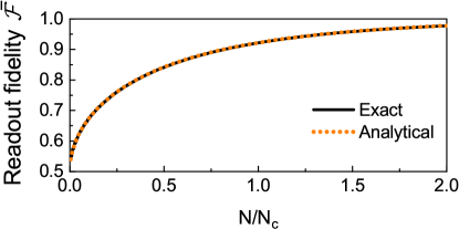
Figure 3: Average readout fidelity $\mathcal{\bar{F}}$ of the multi-outcome measurement as a function of the number $N$ (in units of $N_{\mathrm{c}}\equiv 2/D^{2}$) of constituent binary measurements. Here $\phi=\pi/2$ and $\alpha=0.1$, i.e., the strength of each binary measurement is $D=0.1$.

For finite $N$, the conditional distributions $\mathcal{P}(\bar{u}|\pm\alpha)$ always have a finite overlap. In this case, we can introduce a threshold $\bar{u}_{\mathrm{th}}$ lying between $\langle u\rangle_{\alpha}$ and $\langle u\rangle_{-\alpha}$ [see Fig. 2(c) for an example] and identify the initial state as $|a\rangle$ ($a=\pm\alpha$) if $\bar{u}$ lies on the side of $\langle u\rangle_{a}$. This identification is correct if the outcome $\bar{u}$ lies outside the overlapping region, but it could be incorrect if $\bar{u}$ lies inside the small overlapping region. To quantify its accuracy, we define the readout fidelity $\mathcal{F}_{a}$ of the state $|a\rangle$ ($a=\pm\alpha$) as the probability to identify the initial state to be $|a\rangle$ when the true initial state is $|a\rangle$, e.g., $\mathcal{F}_{\alpha}=\sum_{\bar{u}>\bar{u}_{\mathrm{th}}}\mathcal{P}(\bar{u}|\alpha)$ and $\mathcal{F}_{-\alpha}\equiv\sum_{\bar{u}<\bar{u}_{\mathrm{th}}}\mathcal{P}(\bar{u}|-\alpha)$ for $\langle u\rangle_{\alpha}>\langle u\rangle_{-\alpha}$. Ideal projective measurement corresponds to $\mathcal{F}_{\pm\alpha}=1$. Following Refs. Robledo et al. (2011); Dreau et al. (2013), we maximize the average readout fidelity $\mathcal{\bar{F}}\equiv(\mathcal{F}_{\alpha}+\mathcal{F}_{-\alpha})/2$ by setting $\bar{u}_{\mathrm{th}}$ at the overlapping point, see the vertical dotted lines in Fig. 2(c). For $N\gg 1$, $\mathcal{P}(\bar{u}|\pm\alpha)$ are approximately Gaussian [Eq. (16)], then

$$\bar{u}_{\mathrm{th}}\approx\frac{\langle u\rangle_{\alpha}/\sigma_{\alpha}+\langle u\rangle_{-\alpha}/\sigma_{-\alpha}}{1/\sigma_{\alpha}+1/\sigma_{-\alpha}},$$

so the readout fidelity

$$\mathcal{\bar{F}}=\mathcal{F}_{\pm\alpha}\approx\frac{1}{2}+\frac{1}{2}\mathrm{erf}(\frac{\mathcal{D}}{\sqrt{2}})$$ (18)

is a universal function of the distinguishability $\mathcal{D}$ [Eq. (17)] between $\mathcal{P}(\bar{u}|\pm\alpha)$ or equivalently measurement strength. As shown in Fig. 3, Eq. (18) agrees well with the exact results. When $\mathcal{D}\gtrsim 1$, $\mathcal{\bar{F}}$ approaches 100%, so the multi-outcome measurement approaches an ideal projective measurement. For example, $N=N_{\mathrm{c}}\equiv 2/D^{2}$ leads to $\mathcal{D}=\sqrt{2}$ and hence $\mathcal{\bar{F}}\approx 92\%$, while $N=2N_{\mathrm{c}}$ leads to $\mathcal{D}=2$ and hence $\mathcal{\bar{F}}\approx 98\%$.

For clarity, in the following we define $\mathcal{\bar{F}}_{\mathrm{th}}\equiv 92\%$ or equivalently $\mathcal{D}_{\mathrm{th}}\equiv\sqrt{2}$ as the threshold of a high-fidelity projective measurement.

III.3 Stability analysis

When the QND condition Eq. (14) is violated slightly, the rotation $e^{-i\boldsymbol{\varphi}\cdot\mathbf{\hat{I}}}$ after each binary measurement will rotate the eigenstates $|\pm\alpha\rangle$ of the observable $\hat{\boldsymbol{\alpha}}\cdot\hat{\mathbf{I}}$ slightly away from the measurement axis $\hat{\boldsymbol{\alpha}}$, then the initial state $|\pm\alpha\rangle$ is destroyed after certain number (denoted by $N_{\mathrm{L}}$ – the “lifetime” of $|\pm\alpha\rangle$) of binary measurements. Then the initial state $|\pm\alpha\rangle$ can be measured repeated by at most $N_{\mathrm{L}}$ binary measurements, so the strength of the resulting multi-outcome measurement can reach at most $\mathcal{D}(N_{\mathrm{L}})=\sqrt{N_{\mathrm{L}}}D$. Then constructing a projective measurement above the threshold fidelity $\mathcal{\bar{F}}_{\mathrm{th}}\equiv 92\%$ requires $\mathcal{D}(N_{\mathrm{L}})\geq\mathcal{D}_{\mathrm{th}}\equiv\sqrt{2}$ or equivalently long lifetime

$$N_{\mathrm{L}}\gtrsim N_{\mathrm{c}}\equiv\frac{2}{D^{2}}.$$ (19)

For a quantitative discussion, we calculate the unconditional (i.e., with the measurement outcomes discarded) survival probability of $|\pm\alpha\rangle$ after a sequence of $N$ binary measurements, with the $i$th measurement followed by the rotation $e^{-i\delta\boldsymbol{\varphi}_{i}\cdot\mathbf{\hat{I}}}$. A binary measurement with outcome discarded changes a general nuclear spin state $\hat{\rho}=1/2+\hat{\mathbf{I}}\cdot\mathbf{n}$ with polarization $\mathbf{n}$ into $\sum_{u}\hat{M}_{u}\hat{\rho}\hat{M}_{u}^{\dagger}=1/2+\hat{\mathbf{I}}\cdot\boldsymbol{\mathbb{M}}\mathbf{n}$, where $\boldsymbol{\mathbb{M}}\equiv[\boldsymbol{\mathbb{R}}(\boldsymbol{\alpha})+\boldsymbol{\mathbb{R}}(-\boldsymbol{\alpha})]/2$ describes the measurement-induced dephasing and $\boldsymbol{\mathbb{R}}(\boldsymbol{\theta})$ is the SO(3) rotation matrix as defined after Eq. (11). The effect of $\boldsymbol{\mathbb{M}}$ is to reduce the polarization components perpendicular to $\hat{\boldsymbol{\alpha}}$ by a factor $\cos\alpha$. For clarity we take the initial state as $|\alpha\rangle$. At the end of the evolution, the unconditional nuclear spin state $\hat{\rho}(N)=1/2+\hat{\mathbf{I}}\cdot\hat{\boldsymbol{\alpha}}(N)$ is characterized by the polarization

$$\hat{\boldsymbol{\alpha}}(N)=\boldsymbol{\mathbb{R}}(\delta\boldsymbol{\varphi}_{N})\boldsymbol{\mathbb{M}}\cdots\boldsymbol{\mathbb{R}}(\delta\boldsymbol{\varphi}_{1})\boldsymbol{\mathbb{M}}\hat{\boldsymbol{\alpha}}$$

and the survival probability of $|\alpha\rangle$ is

$$\langle\alpha|\hat{\rho}(N)|\alpha\rangle=\frac{1+\hat{\boldsymbol{\alpha}}\cdot\hat{\boldsymbol{\alpha}}(N)}{2}\equiv\frac{1+S(N)}{2}.$$

For $|-\alpha\rangle$ as the initial state, we obtain the same survival probability. We define the lifetime $N_{\mathrm{L}}$ of $|\pm\alpha\rangle$ as the characteristic $N$ for $S(N)$ to decay to $1/e$. In general, numerical calculations are necessary to determine $S(N)$ and hence $N_{\mathrm{L}}$.

The QND-breaking effect, i.e., the limitation to the lifetime $N_{\mathrm{L}}$, originates from the perpendicular component of $\{\delta\boldsymbol{\varphi}_{i}\}$ with respect to the measurement axis $\hat{\boldsymbol{\alpha}}$. The worst case arises if $\{\delta\boldsymbol{\varphi}_{i}\}$ are all along the same direction (so that different rotations $e^{-i\delta\boldsymbol{\varphi}_{i}\cdot\mathbf{\hat{I}}}$ add up constructively) and this direction is perpendicular to $\hat{\boldsymbol{\alpha}}$ (so that each rotation rotates $|\pm\alpha\rangle$ away from the measurement axis $\hat{\boldsymbol{\alpha}}$ most efficiently). Interestingly, in this worst case, we can obtain analytical results. For clarity we define $\hat{\boldsymbol{\alpha}}$ as the $+X$ axis and $\delta\boldsymbol{\varphi}_{i}$ as the $+Z$ axis, then$\ \delta\boldsymbol{\varphi}_{i}=\delta\varphi_{i}\mathbf{e}_{Z}$. We begin with two special cases:

$$S(N)=\begin{cases}\cos(\sum\limits_{i=1}^{N}(-1)^{i}\delta\varphi_{i})&\cos\alpha=-1,\\ \prod\limits_{i=1}^{N}\cos(\delta\varphi_{i})&\cos\alpha=0.\end{cases}$$

The case $\cos\alpha=-1$ corresponds to $\boldsymbol{\mathbb{M}}=\boldsymbol{\mathbb{R}}(\pi\mathbf{e}_{X})$, i.e., each binary measurement causes $\pi$-rotation of the nuclear spin around the $X$ axis. Then, two binary measurements can reverse a rotation $\boldsymbol{\mathbb{R}}(\delta\varphi\mathbf{e}_{Z})$ around the $Z$ axis: $\boldsymbol{\mathbb{MR}}(\delta\varphi\mathbf{e}_{Z})\boldsymbol{\mathbb{M}}=\boldsymbol{\mathbb{R}}(-\delta\varphi\mathbf{e}_{Z})$. This measurement-induced spin echo can suppress the decay of $S(N)$ when $\delta\varphi_{i}$ varies with $i$ slowly. For $\cos\alpha=0$, the dephasing $\boldsymbol{\mathbb{M}}$ eliminates all the $YZ$ components of the nuclear spin polarization, so the $i$th binary measurement reduces the length of the polarization by a factor $\cos(\delta\varphi_{i})$.

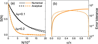
Figure 4: (a) Stability $S(N)$ of $|\alpha\rangle$ against small systematic rotation error for $\boldsymbol{\alpha}=(\pi-0.1)\mathbf{e}_{\pi/4}$ and $\phi=-\pi/2$. (b) Tolerance against systematic error (solid line) and uncorrelated random error (dashed line) for electron spin reaodut fidelity $p=0.1$.

For small systematic rotation error $\delta\varphi_{i}=\delta\varphi\ll\tan^{2}(\alpha/2)$, we obtain $S(N)\approx e^{-N(\delta\varphi)^{2}/[2\tan^{2}(\alpha/2)]}$, which agrees well with the numerical simulations [see Fig. 4(a)]. The lifetime

$$N_{\mathrm{L}}\approx\frac{2}{(\delta\varphi)^{2}}\tan^{2}\frac{\alpha}{2}$$ (20)

depends strongly on $\alpha$ and hence the measurement strength of each binary measurement. When the rotation errors $\{\delta\varphi_{i}\}$ are small uncorrelated random numbers with standard deviation $\delta\varphi$, we obtain $S(N)=e^{-N(\delta\varphi)^{2}/2}$, so the lifetime

$$N_{\mathrm{L}}=\frac{2}{(\delta\varphi)^{2}}$$ (21)

is independent of $\alpha$. The condition Eq. (19) for constructing a projective measurement above the threshold fidelity $\mathcal{\bar{F}}_{\mathrm{th}}\equiv 92\%$ becomes $\delta\varphi\leq\Delta\varphi$, where

$$\Delta\varphi\equiv\left\{\begin{array}[c]{ll}D\left|\tan(\alpha/2)\right|&(\text{systematic error)}\\ D&\text{(uncorrelated random error)}\end{array}\right.,$$ (22)

is the tolerence to rotation errors. As shown in Fig. 4(b), for small $\alpha$, the binary measurement strength $D\propto\alpha$, so the tolerance against systematic (uncorrelated random) rotation error increases quadratically (linearly) with $\alpha$. For $\alpha\rightarrow\pi$, the measurement strength $D\rightarrow 0$ linearly, so the tolerance against uncorrelated random rotation error also approaches zero linearly. By contrast, when $\alpha\rightarrow\pi$, the lifetime $N_{\mathrm{L}}$ due to systematic rotation error diverges quadratically [see Eq. (20)] due to the measurement-induced spin echo, so the tolerance against systematic rotation error approaches a constant $\Delta\varphi\approx 2\bar{p}$ (for $\bar{p}\ll 1$).

When the DD sequence is the repetition of an even-order concatenated DD, the QND condition can be satisfied by tuning $t_{R}$ only, without flipping the electron spin during the waiting time [see the discussions after Eq. (14)]. In this case, we have $\boldsymbol{\varphi}_{R}=(\boldsymbol{\omega}+\mathbf{A}/2)t_{R}$. Then the rotation error $\delta\varphi\sim\delta\varphi_{R}=|\boldsymbol{\omega}+\mathbf{A}/2|\delta t_{R}$ traces back to the error $\delta t_{R}$ in controlling the waiting time. The tolerance against rotation error also translates to the tolerance against the waiting time:

$$\Delta t_{R}\sim\frac{\Delta\varphi}{|\boldsymbol{\omega}+\mathbf{A}/2|}.$$ (23)

IV Example: nitrogen-vacancy center

Parameter sets	P1	P2	P3
Number of CPMG period:$\ N_{\mathrm{DD}}$	$6$	$6$	$8$
Magnetic field $B$	$691$ G	$305$ G	$305$ G
Larmor period $T_{R}\equiv 2\pi/|\omega_{n}|$	$1351$ ns	$3061$ ns	$3061$ ns
Larmor period $T\equiv 2\pi/\left|\boldsymbol{\omega}\right|$	$1088$ ns	$1936$ ns	$1936$ ns

Table 1: Three sets of $(N_{\mathrm{p}},B)$ parameters labelled by P1, P2, and P3. $T$ ($T_{R}$) is the period of the Larmor precession during the DD sequence (waiting time) in the weak hyperfine interaction approximation.

We take an nitrogen-vacancy (NV) center electron spin-1 $\mathbf{\hat{S}}_{\mathrm{NV}}$ coupled to a ¹³C nuclear spin-1/2 $\hat{\mathbf{I}}$ via the hyperfine interaction $\hat{S}_{\mathrm{NV}}^{z}\mathbf{A}\cdot\hat{\mathbf{I}}$ as a paradigmatic physical system to illustrate our method. Under an external magnetic field $B$ along the N-V symmetry axis (defined as the $z$ axis), we can single out two NV electron spin states $|+_{z}\rangle\equiv|m_{S}=0\rangle$ and $|-_{z}\rangle\equiv|m_{S}=-1\rangle$ to form the auxillary electron spin-1/2, e.g., $\hat{S}_{z}\equiv|+_{z}\rangle\langle+_{z}|-|-_{z}\rangle\langle-_{z}|$. Then, in the interaction picture of the electron spin-1/2, we recover the total Hamiltonian in Eq. (1). The hyperfine-shifted nuclear Larmor frequency is $\boldsymbol{\omega}\equiv\omega_{n}\mathbf{e}_{z}-\mathbf{A}/2$, where $\omega_{n}\equiv\gamma_{n}B$ and $\gamma_{n}=-10.71$ MHz/T is the gyromagnetic ratio of the ¹³C nucleus. Next, we follow the standard steps to construct a projective QND measurement on the target ¹³C nucleus.

IV.1 Electron-mediated measurement on ¹³C nucleus

We use the protocol in Fig. 1(a) to construct a single binary measurement on the ¹³C nucleus. We take the DD sequence as the $N_{\mathrm{DD}}$-period CPMG sequence $(\tau/4$-$\pi$-$\tau/2$-$\pi$-$\tau/4)^{N_{\mathrm{DD}}}$ and set $\phi=\pi/2$ (i.e., we measure the electron spin observable $\hat{S}_{y}$) to maximize the strength of each binary measurement. The fidelity of the fluorescence-based readout of the NV center electron spin is determined by the average photon number $n_{\pm}$ for the electron spin state $|\pm_{z}\rangle$ or equivalently the average photon number $\bar{n}=(n_{+}+n_{-})/2$ and the fluorescence contrast $C\equiv(n_{+}-n_{-})/(n_{+}+n_{-})$. Room-temperature experiments have $n_{-}<n_{+}\ll 1$, so nonzero (zero) photon detection corresponds to the outcome $u=+$ ($u=-$). The readout fidelities for $|\pm_{z}\rangle$ are $p_{+}=n_{+}$ and $p_{-}=1-n_{-}$, then $\Delta p=2\bar{n}-1$ and $\bar{p}=2\bar{n}C\ll 1$. Then strength of each binary measurement follows from Eq. (9) as

$$D\approx\sqrt{\bar{n}}C|\sin\alpha|\approx 0.05\left|\sin\alpha\right|,$$ (24)

where we have used typical values $n_{+}=0.1$ and $n_{-}=0.7n_{+}$ or equivalently $\bar{n}=0.085$ and $C=0.18$ in the last step. At low temperature, using resonant optical excitation Robledo et al. (2011); Pfaff et al. (2013); Cramer et al. (2016); Kalb et al. (2016); Reiserer et al. (2016); Yang et al. (2016) gives $n_{+}\gg n_{-}$ and hence much higher readout fidelities on the NV electron spin, then Eq. (9) gives

$$D\sim\bar{p}|\sin\alpha|\approx 0.9\left|\sin\alpha\right|,$$ (25)

where we have used typical values $p_{+}\approx 0.89$ and $p_{-}\approx 0.99$ in the last step. Thus the measurement strength at low temperature is stronger than that at room temperature by a factor $\sim 18$. For specificity, here we consider experiments at room temperature.

IV.2 QND condition and controlling parameters

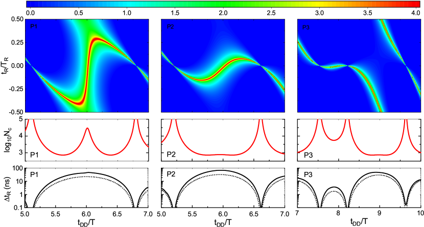
Figure 5: Upper pannels: contour of $\log_{10}N_{\mathrm{L}}$ for P1-P3 in the $(t_{\mathrm{DD}}/T,t_{R}/T_{R}$) plane. Middle and lower panels: $\log_{10}N_{\mathrm{c}}$ and error tolerance $\Delta t_{R}$ as function of $t_{\mathrm{DD}}/T$. The worst-case estimation for $\Delta t_{R}$ is shown as the dashed lines.

We use the protocol in Fig. 1(c) to make each binary measurement QND. According to the discussions after Eq. (14), after measuring the electron spin, we immediately re-initialize the electron spin into $|+_{z}\rangle=|m_{S}=0\rangle$ and then let the ¹³C nuclear spin undergo free precession $e^{-i\boldsymbol{\varphi}_{R}\cdot\mathbf{\hat{I}}}=e^{-i\omega_{n}t_{R}\hat{I}_{z}}$ during the waiting time $t_{R}$. The total rotation of the nuclear spin after the binary measurement is $e^{-i\boldsymbol{\varphi}\cdot\mathbf{\hat{I}}}\equiv e^{-i\omega_{n}t_{R}\hat{I}_{z}}e^{-i\boldsymbol{\varphi}_{\mathrm{DD}}\cdot\mathbf{\hat{I}}}$. By varying $t_{R}$, we can tune $\boldsymbol{\varphi}$ towards the QND condition Eq. (14) to provide a sufficiently long lifetime $N_{\mathrm{L}}\geq N_{\mathrm{c}}$ [Eq. (19)], so that we can use $N_{\mathrm{L}}$ repeated binary measurements to form a multi-outcome projective measurement with readout fidelity above the threshold $\mathcal{F}_{\mathrm{th}}\equiv 92\%$.

The binary measurement is controlled by $\boldsymbol{\alpha}$, which depends on the hyperfine interaction $\mathbf{A}$, the magnetic field $B$, the number $N_{\mathrm{DD}}$ of CPMG periods, and the duration $\tau$ of each period. For specificity, we set $\mathbf{A}=(0.316/\sqrt{2},0.316/\sqrt{2},0.330)$ $\mathrm{MHz}$ Liu et al. (2017) with $1$ $\mathrm{MHz}\equiv 2\pi\times 10^{6}$ rad/(s T) and consider three sets of $(N_{\mathrm{DD}},B$), as labelled by P1, P2, and P3 in Table 1. For each set, we still have two controlling parameters: the CPMG sequence period $\tau$ (or equivalently the CPMG sequence duration $t_{\mathrm{DD}}\equiv N_{\mathrm{DD}}\tau$) and the waiting time $t_{R}$. With $T\equiv 2\pi/|\boldsymbol{\omega}|$ and $T_{R}\equiv 2\pi/|\omega_{n}|$ as the Larmor period of the target ¹³C nucleus during the CPMG sequence and the waiting time, respectively, we can first tune $\tau$ close to resonance with $T$ (or equivalently $t_{\mathrm{DD}}$ close to $N_{\mathrm{DD}}T$) to single out the target ¹³C from other environmental nuclei and then tune $t_{R}$ (or fine tune $\tau$) over one period $[-T_{R}/2,T_{R}/2]$ to search for large $N_{\mathrm{L}}$. Next we perform a numerical simulation for its error tolerance.

IV.3 Numerical simulation

For each set of $(N_{\mathrm{DD}},B$), we scan $t_{R}$ over one period $[-T_{R}/2,T_{R}/2]$ and scan $t_{\mathrm{DD}}\equiv N_{\mathrm{DD}}\tau$ (by scanning $\tau$) in the vicinity of the resonance point $N_{\mathrm{DD}}T$. The lifetime $N_{\mathrm{L}}$ for P1-P3 is shown in the upper panels of Fig. 5. The center of the red region correspond to diverging $N_{\mathrm{L}}$ and hence the exact QND condition. Constructing a projective measurement with readout fidelity above the threshold $\mathcal{\bar{F}}_{\mathrm{th}}\equiv 92\%$ requires long lifetime $N_{\mathrm{L}}\geq N_{\mathrm{c}}$ [Eq. (19)], where $N_{\mathrm{c}}$ as a function of $t_{\mathrm{DD}}$ for P1-P3 is shown in the middle panel of Fig. 5. For each given $t_{\mathrm{DD}}$ in the $(t_{\mathrm{DD}},t_{R})$ plane, the width of the high-fidelity region (in which $N_{\mathrm{L}}\geq N_{\mathrm{c}}$) along the $t_{R}$ axis, i.e., the tolerance $\Delta t_{R}$ against systematic control error of $t_{R}$, is shown in the lower panel of Fig. 5. The worst-case estimation (dashed lines)

$$\Delta t_{R}\sim\frac{T_{R}\ }{\pi}\sqrt{\bar{n}}C\sin^{2}\frac{\alpha}{2}$$

based on Eqs. (22)-(24) shows qualitatively similar dependences on the CPMG duration $t_{\mathrm{DD}}$ as the exact numerical results, but it significantly underestimate $\Delta t_{R}$, in agreement with our discussions in Sec. III.3. The error tolerance $\Delta t_{R}$ are on the nanoseconds time scale, within reach of typical experiments. Therefore, constructing projective QND measurements from a sequence of binary measurements is possible for P1-P3. Moreover, if we work at low temperatures and use resonant optical excitation for high-fidelity readout of the NV electron spin, then we can further enhance $D$ and hence the error tolerance by a factor of $\sim 18$.

V Conclusion

We have developed a general theory for constructing projective quantum nondemolition (QND) measurement on an arbitrary nuclear spin-1/2 by measuring an axillary electron spin in generic electron-nuclear spin systems coupled via hyperfine interaction. A distinguishing feature is that the QND observable is not conserved during the free Larmor precession of the nuclear spin and can be tuned in situ. The key idea consists of three steps. First, suitable dynamical decoupling control on the electron is used to design the electron-nuclear entanglement and hence select the nuclear spin observable to be measured. Second, the nuclear spin evolution between neighboring measurements is tuned to make the measurement QND. Finally, a sequence of such measurements are cascaded into a projective QND measurement. We identify tunable parameters to control the QND observable and further find optimal parameters that stabilize the QND measurement against experimental control errors. This work provides a paradigm for building up QND measurement on non-conserved observables by a sequence of non-projective measurements in hybrid qubit systems, which may be relevant to the state preparation, quantum sensing, and quantum error correction via projective QND measurements. The formalisms developed here can also be used to design other QND measurements via more general quantum controls or study other measurement backaction effect in NV center and other solid-state spin systems, such as semiconductor quantum dots and phosphorus and bismuth donors in silicon.

Note added—- Recently, Ref.Ma et al. (2022) discuss how a sequence of mutually commuting, normal POVM (which is precisely the QND condition discussed in our paper) cascade into a projective measurement and provide a simple example based on a toy model. Here we focus on a realistic physical system – electron-nuclear spin systems coupled through realistic hyperfine interaction. In this system, the electron-mediated measurement on the nuclear spin is not QND, in construct to Ref. Ma et al. (2022). We show how to use suitable quantum control to engineer such non-QND measurements into QND ones, how to tune the QND observables and control the strength of the QND measurements, how a sequence of such QND measurements cascade into a projective measurement, and how the QND measurement is stabilized against realistic experimental control errors. We also give an explicit scheme for constructing a projective QND measurement on a 13C nuclear spin weakly coupled to a nitrogen-vacancy center electron spin in diamond.

Appendix A Evolution during DD sequence

We assume the DD sequence consists of $N$ $\pi$-pulses at $t_{1}\leq t_{2}\leq\cdots\leq t_{N}$. During the DD sequence, the total Hamiltonian in the interaction picture of the auxiliary electron is

$$\hat{H}(t)=[\boldsymbol{\omega}+s(t)\hat{S}_{z}\mathbf{A}]\cdot\hat{\mathbf{I}},$$ (26)

where the DD modulation function $s(t)$ starts from $s(0)=+1$ and switches its sign at $t_{1},t_{2},\cdots,t_{N}$ Cywinski et al. (2008); Yang et al. (2017). The evolution operator during the DD sequence is $e^{-i\boldsymbol{\omega}_{\mathrm{f}}\cdot\mathbf{\hat{I}(}t_{\mathrm{p}}-t_{N})}\cdots e^{-i\boldsymbol{\omega}_{\pm}\cdot\mathbf{\hat{I}(}t_{3}-t_{2})}e^{-i\boldsymbol{\omega}_{\mp}\cdot\mathbf{\hat{I}(}t_{2}-t_{1})}e^{-i\boldsymbol{\omega}_{\pm}\cdot\hat{\mathbf{I}}t_{1}}$

$$\hat{U}_{\mathrm{DD}}=e^{-i(\boldsymbol{\omega}+(-1)^{N}\hat{S}_{z}\mathbf{A})\cdot\hat{\mathbf{I}}}\cdots e^{-i(\boldsymbol{\omega}-\hat{S}_{z}\mathbf{A})\cdot\hat{\mathbf{I}}}e^{-i(\boldsymbol{\omega}+\hat{S}_{z}\mathbf{A})\cdot\hat{\mathbf{I}}}.$$ (27)

We can expand $\hat{U}_{\mathrm{DD}}$ using the eigenstates $|\pm_{z}\rangle$ of $\hat{S}_{z}$ as

$$\hat{U}_{\mathrm{DD}}=\hat{U}_{\mathrm{DD}}^{(+)}|+_{z}\rangle\langle+_{z}|+\hat{U}_{\mathrm{DD}}^{(-)}|-_{z}\rangle\langle-_{z}|,$$

where $\hat{U}_{\mathrm{DD}}^{(\pm)}=(\hat{U}_{\mathrm{DD}})_{\hat{S}_{z}\rightarrow\pm 1/2}$ are nuclear spin evolution operators for the electron spin initial state $|\pm_{z}\rangle$. Next we define $\boldsymbol{\alpha}$ and $\boldsymbol{\varphi}_{\mathrm{DD}}$ via

$$e^{2i\boldsymbol{\alpha}\cdot\mathbf{\hat{I}}} \equiv(\hat{U}_{\mathrm{DD}}^{(+)})^{\dagger}\hat{U}_{\mathrm{DD}}^{(-)},$$

$$e^{-i\boldsymbol{\varphi}_{\mathrm{DD}}\cdot\mathbf{\hat{I}}} \equiv\hat{U}_{\mathrm{DD}}^{(+)}e^{i\boldsymbol{\alpha}\cdot\mathbf{\hat{I}}}=\hat{U}_{\mathrm{DD}}^{(-)}e^{-i\boldsymbol{\alpha}\cdot\mathbf{\hat{I}}},$$

then $\hat{U}_{\mathrm{DD}}^{(\pm)}=e^{-i\boldsymbol{\varphi}_{\mathrm{DD}}\cdot\mathbf{\hat{I}}}e^{\mp i\boldsymbol{\alpha}\cdot\mathbf{\hat{I}}}$ and we obtain Eq. (2) in the main text.

Appendix B Weak hyperfine interaction

The evolution operator during the DD sequence [Eq. (27)] can be written as

$$\hat{U}_{\mathrm{DD}}=e^{-i\boldsymbol{\omega}\cdot\hat{\mathbf{I}}t_{\mathrm{DD}}}\mathcal{T}e^{-i\hat{S}_{z}\int_{0}^{t_{\mathrm{DD}}}s(t)\mathbf{A}\cdot\hat{\mathbf{I}}(t)dt^{\prime}},$$

where $\mathcal{T}$ is the time-ordering superoperator and $\mathbf{\hat{I}}(t)\equiv e^{i\boldsymbol{\omega}\cdot\mathbf{\hat{I}}t}\mathbf{\hat{I}}e^{-i\boldsymbol{\omega}\cdot\mathbf{\hat{I}}t}$. When the perpendicular part $\mathbf{A}_{\perp}$ of $\mathbf{A}$ with respect to $\boldsymbol{\omega}$ is much smaller than the nuclear Zeeman splitting $|\boldsymbol{\omega}|$, we can use the first-order Magus expansion to obtain

$$\hat{U}_{\mathrm{DD}}\approx e^{-i\boldsymbol{\omega}\cdot\mathbf{\hat{I}}t_{\mathrm{DD}}}e^{-i\hat{S}_{z}\int_{0}^{t_{\mathrm{DD}}}s(t)\mathbf{A}\cdot\mathbf{\hat{I}}(t)dt}.$$

For convenience we define $\boldsymbol{\omega}$ as the $z$ axis ($\boldsymbol{\omega}=\omega\mathbf{e}_{z}$) and decompose $\mathbf{A}$ into $A_{z}\mathbf{e}_{z}$ and $\mathbf{A}_{\perp}=A_{\perp}(\cos\Phi\mathbf{e}_{x}+\sin\Phi\mathbf{e}_{y})=A_{\perp}\operatorname{Re}\mathbf{e}_{+}e^{-i\Phi}$ ($\mathbf{e}_{\pm}\equiv\mathbf{e}_{x}\pm i\mathbf{e}_{y}$), then $\mathbf{A}\cdot\mathbf{\hat{I}}(t)=A_{z}\hat{I}_{z}+A_{\perp}\mathbf{\hat{I}\cdot}\operatorname{Re}\mathbf{e}_{+}e^{-i\Phi}e^{i\omega t}$. For a DD sequence of duration $t_{\mathrm{DD}}$, the modulation function must satisfy $\int_{0}^{t_{\mathrm{DD}}}s(t)dt=0$, thus the term $A_{z}\hat{I}_{z}$ is averaged out, and

$$\hat{U}_{\mathrm{DD}}\approx e^{-\omega t_{\mathrm{DD}}\hat{I}_{z}}e^{-i\hat{S}_{z}t_{\mathrm{DD}}A_{\perp}\mathbf{\hat{I}}\cdot\operatorname{Re}\mathbf{e}_{+}e^{-i\Phi}f_{\mathrm{DD}}}\newline \newline =e^{-it_{\mathrm{DD}}(\boldsymbol{\omega}\cdot\mathbf{\hat{I}})}e^{-i2\hat{S}_{z}\boldsymbol{\alpha}\cdot\mathbf{\hat{I}}},$$

where $f_{\mathrm{DD}}$ is given by Eq. (12) and $\boldsymbol{\alpha}$ is given by Eq. (11).

Appendix C Stroboscopic QND condition for even-order concatenated DD sequences

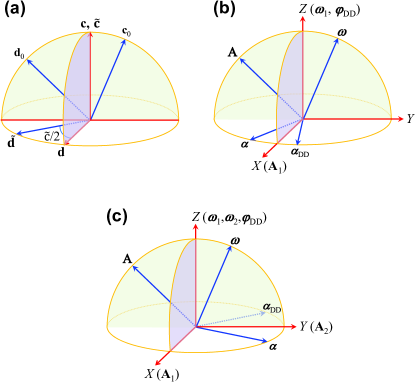
Figure 6: (a) Orientation of relevant vectors for Eqs. (29) and (30). (b) Orientations of relevant vectors for the periodic DD. (c) Orientations of relevant vectors for the CPMG sequence.

The QND condition Eq. (14) is equivalent to

$$\mathbb{R}(\boldsymbol{\varphi}_{R})\hat{\boldsymbol{\alpha}}_{\mathrm{DD}}=\hat{\boldsymbol{\alpha}},$$ (28)

where $\hat{\boldsymbol{\alpha}}_{\mathrm{DD}}\equiv\mathbb{R}(\boldsymbol{\varphi}_{\mathrm{DD}})\hat{\boldsymbol{\alpha}}$ is obtained from $\hat{\boldsymbol{\alpha}}$ by a rotation around the axis $\boldsymbol{\varphi}_{\mathrm{DD}}$ by an angle $|\boldsymbol{\varphi}_{\mathrm{DD}}|$. This can be achieved by first tuning the direction of $\boldsymbol{\varphi}_{R}$ into the bisection plane of $\hat{\boldsymbol{\alpha}}$ and $\hat{\boldsymbol{\alpha}}_{\mathrm{DD}}$ and then tuning $|\boldsymbol{\varphi}_{R}|$ to satisfy Eq. (28). As discussed in the main text, we can achieve an arbitrary evolution $e^{-i\boldsymbol{\varphi}_{R}\cdot\mathbf{\hat{I}}}$ by tuning $t_{R}$ and the timings of the electron spin flip during the waiting time $t_{R}$, so Eq. (28) can always be satisfied. Next, we further prove that when the DD sequence is the repetition of an even-order concatenated DD Khodjasteh and Lidar (2005); Yao et al. (2007); Khodjasteh and Lidar (2007); Yang et al. (2011), the QND condition can be achieved by the evolution $e^{-i\boldsymbol{\varphi}_{R}\cdot\mathbf{\hat{I}}}=e^{-i(\boldsymbol{\omega}+\mathbf{A}/2)t_{R}\cdot\mathbf{\hat{I}}}$ at suitable $t_{R}$, i.e., for these DD sequences, the QND condition can be satisfied by tuning the duration $t_{R}$ of the waiting interval, without flipping the electron spin during the waiting interval.

We will use repeatedly two important properties (with $\hat{S}_{z}$ for the electron spin-1/2 and $\mathbf{\hat{I}}$ for the target nuclear spin-1/2): (i) Given arbitrary vectors $\mathbf{c}_{0}$ and $\mathbf{d}_{0}$, if we define $\mathbf{c}$ and $\mathbf{d}$ via

$$e^{-i(\mathbf{c}+\hat{S}_{z}\mathbf{d})\cdot\mathbf{\hat{I}}}=e^{-i\mathbf{(c}_{0}-\hat{S}_{z}\mathbf{d}_{0})\cdot\mathbf{\hat{I}}}e^{-i(\mathbf{c}_{0}+\hat{S}_{z}\mathbf{d}_{0})\cdot\mathbf{\hat{I}}},$$ (29)

then $\mathbf{c}$ lies in the $\mathbf{c}_{0}$-$\mathbf{d}_{0}\$plane ($\mathbf{c}\parallel\mathbf{c}_{0}$ if $\mathbf{c}_{0}\perp\mathbf{d}_{0}$), while $\mathbf{d\parallel c}_{0}\times\mathbf{d}_{0}$, as shown in Fig. 6(a). (ii) Given two orthogonal vectors $\mathbf{c}\perp\mathbf{d}$, if we define $\mathbf{\tilde{c}}$ and $\mathbf{\tilde{d}}$ via

$$e^{-i\mathbf{\tilde{c}}\cdot\mathbf{\hat{I}}}e^{-i2\hat{S}_{z}\mathbf{\tilde{d}}\cdot\mathbf{\hat{I}}}=e^{-i(\mathbf{c}+\hat{S}_{z}\mathbf{d})\cdot\mathbf{\hat{I}}},$$ (30)

then $\mathbf{\tilde{c}}\parallel\mathbf{c}$ and $\mathbf{\tilde{d}}\parallel\mathbb{R}(-\mathbf{\tilde{c}}/2)\mathbf{d}$, as shown in Fig. 6(a). The proof will be given at the end of this appendix.

To illustrate the concept of concatenation, we begin with the periodic DD $(\tau/4$-$\pi$-$\tau/4$-$\pi$)^N consisting of $N$ periods. The evolution operator $\hat{U}_{1}$ of the electron-nuclear system in one period is the concatenation of the free evolution $\hat{U}_{0}\equiv e^{-i(\tau/4)(\boldsymbol{\omega}+\hat{S}_{z}\mathbf{A})\cdot\mathbf{\hat{I}}}$, i.e.,

$$\hat{U}_{1}\equiv(\hat{U}_{0})_{\hat{S}_{z}\rightarrow-\hat{S}_{z}}\hat{U}_{0},$$ (31)

and the total evolution during this DD sequence is $\hat{U}_{\mathrm{DD}}=\hat{U}_{1}^{N}$. Namely, this periodic DD consists of $N$ repetitions of the first-order concatenated DD. Using Eq. (29), we have

$$\hat{U}_{1} =e^{-i(\tau/2)(\boldsymbol{\omega}_{1}+\hat{S}_{z}\mathbf{A}_{1}/2)\cdot\mathbf{\hat{I}}},$$

$$\hat{U}_{\mathrm{DD}} =e^{-i(N\tau/2)(\boldsymbol{\omega}_{1}+\hat{S}_{z}\mathbf{A}_{1}/2)\cdot\mathbf{\hat{I}}},$$

where $\boldsymbol{\omega}_{1}$ lies in the $\boldsymbol{\omega}$-$\mathbf{A}$ plane and $\mathbf{A}_{1}\parallel\boldsymbol{\omega}\times\mathbf{A}$. For convenience, we define $\mathbf{A}_{1}$ as the $X$ axis, the $\boldsymbol{\omega}$-$\mathbf{A}$ plane as the $YZ$ plane, and $\boldsymbol{\omega}_{1}$ as the $Z$ axis, as shown in Fig. 6(b). Next we can use Eq. (30) to obtain $\hat{U}_{\mathrm{DD}}=e^{-i\boldsymbol{\varphi}_{\mathrm{DD}}\cdot\mathbf{\hat{I}}}e^{-i2\hat{S}_{z}\boldsymbol{\alpha}\cdot\mathbf{\hat{I}}}$ with $\boldsymbol{\varphi}_{\mathrm{DD}}$ along the $Z$ axis and $\boldsymbol{\hat{\alpha}}$ in the $XY$ plane with azimuth $-|\boldsymbol{\varphi}_{\mathrm{DD}}|/2$, so $\hat{\boldsymbol{\alpha}}_{\mathrm{DD}}$ also lies in the $XY$ plane with azimuth $|\boldsymbol{\varphi}_{\mathrm{DD}}|/2$, i.e., $\boldsymbol{\hat{\alpha}}$ and $\hat{\boldsymbol{\alpha}}_{\mathrm{DD}}$ lie symmetrically about $\mathbf{A}_{1}$ in the $XY$ plane, as shown in Fig. 6(b). Therefore, for the periodic DD, the evolution $e^{-i\boldsymbol{\varphi}_{R}\cdot\mathbf{\hat{I}}}=e^{-i(\boldsymbol{\omega}+\mathbf{A}/2)t_{R}\cdot\mathbf{\hat{I}}}$ cannot satisfy the QND condition.

Next we consider the CPMG sequence $(\tau/4$-$\pi$-$\tau/2$-$\pi$-$\tau/4$)^N consisting of $N$ periods. The evolution operator of the electron-nuclear system during one period is the concatenation of $\hat{U}_{1}$ [Eq. (31)], i.e.,

$$\hat{U}_{2}\equiv(\hat{U}_{1})_{\hat{S}_{z}\rightarrow-\hat{S}_{z}}\hat{U}_{1},$$

and the total evolution during the CPMG sequence is $\hat{U}_{\mathrm{DD}}=\hat{U}_{2}^{N}$. Namely, this CPMG sequence consists of $N$ repetitions of the second-order concatenated DD. Using Eq. (29), we obtain

$$\hat{U}_{2}=e^{-i\tau(\boldsymbol{\omega}_{2}+\hat{S}_{z}\mathbf{A}_{2}/2)\cdot\mathbf{\hat{I}}},$$

with $\boldsymbol{\omega}_{2}$ along the $Z$ axis and $\mathbf{A}_{2}$ along the $Y$ axis. Next we use Eq. (30) to obtain $\hat{U}_{\mathrm{DD}}=e^{-i\boldsymbol{\varphi}_{\mathrm{DD}}\cdot\mathbf{\hat{I}}}e^{-i2\hat{S}_{z}\boldsymbol{\alpha}\cdot\mathbf{\hat{I}}}$ with $\boldsymbol{\varphi}_{\mathrm{DD}}$ along the $Z$ axis and $\boldsymbol{\hat{\alpha}}$ in the $XY$ plane with azimuth $\pi/2-|\boldsymbol{\varphi}_{\mathrm{DD}}|/2$, so $\hat{\boldsymbol{\alpha}}_{\mathrm{DD}}$ also lies in the $XY$ plane with azimuth $\pi/2+|\boldsymbol{\varphi}_{\mathrm{DD}}|/2$, i.e., $\boldsymbol{\hat{\alpha}}$ and $\hat{\boldsymbol{\alpha}}_{\mathrm{DD}}$ lie symmetrically about $\mathbf{A}_{2}$ in the $XY$ plane [see Fig. 6(c)]. Then the evolution $e^{-i\boldsymbol{\varphi}_{R}\cdot\mathbf{\hat{I}}}=e^{-i(\boldsymbol{\omega}+\mathbf{A}/2)\cdot\mathbf{\hat{I}}t_{R}}$ can satisfy the stroboscopic QND condition at suitable $t_{R}$, i.e., without flipping the electron spin during the waiting time.

The concatenation process can be carried out to higher order to obtain the period

$$\hat{U}_{l}\equiv(\hat{U}_{l-1})_{\hat{S}_{z}\rightarrow-\hat{S}_{z}}\hat{U}_{l-1}$$

of the $l$th-order concatenated DD Khodjasteh and Lidar (2005); Yao et al. (2007); Khodjasteh and Lidar (2007); Yang et al. (2011). If the DD sequence consists of $N$ repetitions of $\hat{U}_{l}$, then the total evolution is $\hat{U}_{\mathrm{DD}}=\hat{U}_{l}^{N}$. Using Eq. (29), we obtain

$$\hat{U}_{l}=e^{-i2^{l-2}N\tau(\boldsymbol{\omega}_{l}+\hat{S}_{z}\mathbf{A}_{l})\cdot\mathbf{\hat{I}}},$$

with $\boldsymbol{\omega}_{l}$ along the $Z$ axis and $\mathbf{A}_{l}$ in the $XY$ plane with azimuth $(l-1)\pi/2$. Next we can use Eq. (30) to obtain $\hat{U}_{\mathrm{DD}}=e^{-i\boldsymbol{\varphi}_{\mathrm{DD}}\cdot\mathbf{\hat{I}}}e^{-i2\hat{S}_{z}\boldsymbol{\alpha}\cdot\mathbf{\hat{I}}}$, where $\boldsymbol{\varphi}_{\mathrm{DD}}$ is along the $Z$ axis and $\boldsymbol{\hat{\alpha}}$ in the $XY$ plane with azimuth $(l-1)\pi/2-|\boldsymbol{\varphi}_{\mathrm{DD}}|/2$, so $\hat{\boldsymbol{\alpha}}_{\mathrm{DD}}$ also lies in the $XY$ plane with azimuth $(l-1)\pi/2+|\boldsymbol{\varphi}_{\mathrm{DD}}|/2$, i.e., $\boldsymbol{\hat{\alpha}}$ and $\hat{\boldsymbol{\alpha}}_{\mathrm{DD}}$ lie symmetrically about $\mathbf{A}_{l}$ in the $XY$ plane. For even $l$, $\mathbf{A}_{l}$ is along the $\pm Y$ axis, so the evolution $e^{-i\boldsymbol{\varphi}_{R}\cdot\mathbf{\hat{I}}}=e^{-i(\boldsymbol{\omega}+\mathbf{A}/2)\cdot\mathbf{\hat{I}}t_{R}}$ can satisfy the stroboscopic QND condition at suitable $t_{R}$, i.e., without flipping the electron spin during the waiting time.

Finally we prove properties (i) and (ii). For property (i), we notice that Eq. (29) is equivalent to

$$e^{-i(\mathbf{c}\pm\mathbf{d}/2)\cdot\mathbf{\hat{I}}}=e^{-i\mathbf{(c}_{0}\mp\mathbf{d}_{0}/2)\cdot\mathbf{\hat{I}}}e^{-i(\mathbf{c}_{0}\pm\mathbf{d}_{0}/2)\cdot\mathbf{\hat{I}}},$$

which further becomes

$$e^{-i(\mathbf{C}\pm\mathbf{D})\cdot\boldsymbol{\sigma}}=e^{-i\mathbf{a}_{\mp}\cdot\boldsymbol{\sigma}}e^{-i\mathbf{a}_{\pm}\cdot\boldsymbol{\sigma}}$$

by using $\mathbf{\hat{I}}=\boldsymbol{\sigma}/2$ ($\boldsymbol{\sigma}$ are Pauli matrices) and defining $\mathbf{C}\equiv\mathbf{c}/2,$ $\mathbf{D}=\mathbf{d}/4$, and $\mathbf{a}_{\pm}\equiv(\mathbf{c}_{0}\pm\mathbf{d}_{0}/2)/2$. Using $e^{-i\theta(\mathbf{e}\cdot\boldsymbol{\sigma})}=\cos\theta-i\boldsymbol{\sigma}\cdot\sin(\theta\mathbf{e})$ [$\mathbf{e}$ is a unit vector and $\sin(\theta\mathbf{e})\equiv\mathbf{e}\sin\theta$], we obtain

$$\cos\left|\mathbf{C}\pm\mathbf{D}\right| =\cos a_{+}\cos a_{-}-\sin\mathbf{a}_{+}\cdot\sin\mathbf{a}_{-},$$

$$\sin(\mathbf{C}\pm\mathbf{D}) =\cos a_{+}\sin\mathbf{a}_{-}+\sin\mathbf{a}_{+}\cos a_{-}\pm\sin\mathbf{a}_{-}\mathbf{\times}\sin\mathbf{a}_{+},$$

where $a_{\pm}=|\mathbf{a}_{\pm}|$. The first equation dictates $\left|\mathbf{C}+\mathbf{D}\right|=\left|\mathbf{C}-\mathbf{D}\right|$, then we can substitute $\sin(\mathbf{C}\pm\mathbf{D})=(\mathbf{C}\pm\mathbf{D})\operatorname{sinc}\sqrt{C^{2}+D^{2}}$ into the second equation to obtain $\mathbf{C\propto}\sin\mathbf{a}_{-}\cos a_{+}+\sin\mathbf{a}_{+}\cos a_{-}$ and $\mathbf{D}\propto\sin\mathbf{a}_{-}\times\sin\mathbf{a}_{+}$. In other words, $\mathbf{C}$ lies in the $\mathbf{a}_{+}$-$\mathbf{a}_{-}\$plane ($\mathbf{C}\parallel\mathbf{a}_{+}+\mathbf{a}_{-}$ if $a_{+}=a_{-}$), while $\mathbf{D\parallel a}_{-}\times\mathbf{a}_{+}$. This proves property (i).

Similarly, Eq. (30) is equivalent to

$$e^{-i\mathbf{\tilde{c}}\cdot\mathbf{\hat{I}}}e^{\mp i\mathbf{\tilde{d}}\cdot\mathbf{\hat{I}}}=e^{-i(\mathbf{c}\pm\mathbf{d}/2)\cdot\mathbf{\hat{I}}},$$

which further becomes

$$e^{-i\mathbf{\tilde{C}}\cdot\boldsymbol{\sigma}}e^{\mp i\mathbf{\tilde{D}}\cdot\boldsymbol{\sigma}}=e^{-i(\mathbf{C}\pm\mathbf{D})\cdot\boldsymbol{\sigma}}$$

with $\mathbf{C}=\mathbf{c}/2,$ $\mathbf{D}=\mathbf{d}/4$, $\mathbf{\tilde{C}}=\mathbf{\tilde{c}}/2$, and $\mathbf{\tilde{D}}=\mathbf{\tilde{d}}/2$. Using $e^{-i\theta(\mathbf{e}\cdot\boldsymbol{\sigma})}=\cos\theta-i\boldsymbol{\sigma}\cdot\sin(\theta\mathbf{e})$, we obtain

$$\cos\sqrt{C^{2}+D^{2}} =\cos\tilde{C}\cos\tilde{D}\mp\sin\mathbf{\tilde{C}\cdot}\sin\mathbf{\tilde{D},}$$

$$(\mathbf{C}\pm\mathbf{D})\operatorname{sinc}\sqrt{C^{2}+D^{2}} =\sin\mathbf{\tilde{C}}\cos\tilde{D}\pm\sin\mathbf{\tilde{D}}\cos\tilde{C}\pm\sin\mathbf{\tilde{C}\times}\sin\mathbf{\tilde{D}.}$$

The first equation dictates $\mathbf{\tilde{C}}\perp\mathbf{\tilde{D}}$. The second equation gives $\mathbf{C}\propto\sin\mathbf{\tilde{C}}$ and $\mathbf{D}\propto\sin\mathbf{\tilde{D}}\cos\tilde{C}+\sin\mathbf{\tilde{C}\times}\sin\mathbf{\tilde{D}}=\mathbb{R}(\mathbf{\tilde{C}})\sin\mathbf{\tilde{D}}$, so $\mathbf{\tilde{C}}\parallel\mathbf{C}$ and $\mathbf{\tilde{D}}\parallel\mathbb{R}(-\mathbf{\tilde{C}})\mathbf{D}$. This proves property (ii).

References

- Wiseman and Milburn (2010) H. M. Wiseman and G. J. Milburn, Quantum measurement and control (Cambridge University Press, 2010).
- Braginsky and Vorontsov (1975) V. B. Braginsky and Y. I. Vorontsov, Soviet Physics Uspekhi 17, 644 (1975).
- Braginskii et al. (1977) V. Braginskii, Y. I. Vorontsov, and F. Y. Khalili, Sov. Phys. JETP 46, 705 (1977).
- Thorne et al. (1978) K. S. Thorne, R. W. P. Drever, C. M. Caves, M. Zimmermann, and V. D. Sandberg, Phys. Rev. Lett. 40, 667 (1978).
- Unruh (1979) W. G. Unruh, Phys. Rev. D 19, 2888 (1979).
- Caves et al. (1980) C. M. Caves, K. S. Thorne, R. W. P. Drever, V. D. Sandberg, and M. Zimmermann, Rev. Mod. Phys. 52, 341 (1980).
- Braginsky et al. (1980) V. B. Braginsky, Y. I. Vorontsov, and K. S. Thorne, Science 209, 547 (1980).
- Clerk et al. (2010) A. A. Clerk, M. H. Devoret, S. M. Girvin, F. Marquardt, and R. J. Schoelkopf, Rev. Mod. Phys. 82, 1155 (2010).
- Grangier et al. (1998) P. Grangier, J. A. Levenson, and J.-P. Poizat, Nature 396, 537 (1998).
- Lupascu et al. (2007) A. Lupascu, S. Saito, T. Picot, P. C. de Groot, C. J. P. M. Harmans, and J. E. Mooij, Nat. Phys. 3, 119 (2007).
- Peil and Gabrielse (1999) S. Peil and G. Gabrielse, Phys. Rev. Lett. 83, 1287 (1999).
- Laraoui et al. (2013) A. Laraoui, F. Dolde, C. Burk, F. Reinhard, J. Wrachtrup, and C. A. Meriles, Nature Communications 4, 1651 (2013).
- Staudacher et al. (2015) T. Staudacher, N. Raatz, S. Pezzagna, J. Meijer, F. Reinhard, C. A. Meriles, and J. Wrachtrup, Nat. Commun. 6, (2015).
- Mamin et al. (2013) H. J. Mamin, M. Kim, M. H. Sherwood, C. T. Rettner, K. Ohno, D. D. Awschalom, and D. Rugar, Science 339, 557 (2013).
- Wang et al. (2017) Z.-Y. Wang, J. Casanova, and M. B. Plenio, Nat. Commun. 8, 14660 (2017).
- Zaiser et al. (2016) S. Zaiser, T. Rendler, I. Jakobi, T. Wolf, S.-Y. Lee, S. Wagner, V. Bergholm, T. Schulte-Herbrüggen, P. Neumann, and J. Wrachtrup, Nature Communications 7, 12279 (2016).
- Shi et al. (2014) F. Shi, X. Kong, P. Wang, F. Kong, N. Zhao, R.-B. Liu, and J. Du, Nat. Phys. 10, 21 (2014).
- Shi et al. (2015) F. Shi, Q. Zhang, P. Wang, H. Sun, J. Wang, X. Rong, M. Chen, C. Ju, R. Friedemann, J. Wang, and J. Du, Science 347, 1135 (2015).
- Du et al. (2009) J. Du, X. Rong, N. Zhao, Y. Wang, J. Yang, and R. B. Liu, Nature 461, 1265 (2009).
- Pfender et al. (2017) M. Pfender, N. Aslam, H. Sumiya, S. Onoda, P. Neumann, J. Isoya, C. A. Meriles, and J. Wrachtrup, Nat. Commun. 8, 834 (2017).
- Rosskopf et al. (2017) T. Rosskopf, J. Zopes, J. M. Boss, and C. L. Degen, npj Quantum Inf. 3, 33 (2017).
- Schmitt et al. (2017) S. Schmitt, T. Gefen, F. M. Stürner, T. Unden, G. Wolff, C. Müller, J. Scheuer, B. Naydenov, M. Markham, S. Pezzagna, J. Meijer, I. Schwarz, M. Plenio, A. Retzker, L. P. McGuinness, and F. Jelezko, Science 356, 832 (2017).
- Glenn et al. (2018) D. R. Glenn, D. B. Bucher, J. Lee, M. D. Lukin, H. Park, and R. L. Walsworth, Nature 555, 351 (2018).
- Muhonen et al. (2014) J. T. Muhonen, J. P. Dehollain, A. Laucht, F. E. Hudson, R. Kalra, T. Sekiguchi, K. M. Itoh, D. N. Jamieson, J. C. McCallum, A. S. Dzurak, and A. Morello, Nat Nano 9, 986 (2014).
- Saeedi et al. (2013) K. Saeedi, S. Simmons, J. Z. Salvail, P. Dluhy, H. Riemann, N. V. Abrosimov, P. Becker, H.-J. Pohl, J. J. Morton, and M. L. Thewalt, Science 342, 830 (2013).
- Tyryshkin et al. (2012) A. M. Tyryshkin, S. Tojo, J. J. L. Morton, H. Riemann, N. V. Abrosimov, P. Becker, H.-J. Pohl, T. Schenkel, M. L. W. Thewalt, K. M. Itoh, and S. A. Lyon, Nat. Mater. 11, 143 (2012).
- Press et al. (2010) D. Press, K. De Greve, P. L. McMahon, T. D. Ladd, B. Friess, C. Schneider, M. Kamp, S. Hofling, A. Forchel, and Y. Yamamoto, Nat. Photon. 4, 367 (2010).
- Taminiau et al. (2014) T. H. Taminiau, J. Cramer, T. van der Sar, V. V. Dobrovitski, and R. Hanson, Nat Nano 9, 171 (2014).
- Yang et al. (2016) S. Yang, Y. Wang, D. D. B. Rao, T. Hien Tran, A. S. Momenzadeh, M. Markham, D. J. Twitchen, P. Wang, W. Yang, R. Stöhr, P. Neumann, H. Kosaka, and J. Wrachtrup, Nature Photonics 10, 507 (2016).
- Dreau et al. (2013) A. Dreau, P. Spinicelli, J. R. Maze, J.-F. Roch, and V. Jacques, Phys. Rev. Lett. 110, 060502 (2013).
- Neumann et al. (2010) P. Neumann, J. Beck, M. Steiner, F. Rempp, H. Fedder, P. R. Hemmer, J. Wrachtrup, and F. Jelezko, Science 329, 542 (2010).
- Liu et al. (2017) G.-Q. Liu, J. Xing, W.-L. Ma, P. Wang, C.-H. Li, H. C. Po, Y.-R. Zhang, H. Fan, R.-B. Liu, and X.-Y. Pan, Phys. Rev. Lett. 118, 150504 (2017).
- Braginsky et al. (1978) V. B. Braginsky, Y. I. Vorontsov, and F. Y. Khalili, JETP Lett. 27, 276 (1978).
- Jordan and Büttiker (2005) A. N. Jordan and M. Büttiker, Phys. Rev. B 71, 125333 (2005).
- Ruskov et al. (2005) R. Ruskov, K. Schwab, and A. N. Korotkov, Phys. Rev. B 71, 235407 (2005).
- Jordan et al. (2006) A. N. Jordan, A. N. Korotkov, and M. Büttiker, Phys. Rev. Lett. 97, 026805 (2006).
- Averin et al. (2006) D. V. Averin, K. Rabenstein, and V. K. Semenov, Phys. Rev. B 73, 094504 (2006).
- Jordan and Korotkov (2006) A. N. Jordan and A. N. Korotkov, Phys. Rev. B 74, 085307 (2006).
- Greiner et al. (2017) J. N. Greiner, D. B. R. Dasari, and J. Wrachtrup, Sci. Rep. 7, 529 (2017).
- Cywinski et al. (2008) L. Cywinski, R. M. Lutchyn, C. P. Nave, and S. Das Sarma, Phys. Rev. B 77, 174509 (2008).
- Yang et al. (2017) W. Yang, W.-L. Ma, and R.-B. Liu, Rep. Prog. Phys. 80, 016001 (2017).
- Liu et al. (2010) R.-B. Liu, W. Yao, and L. J. Sham, Adv. Phys. 59, 703 (2010).
- Khodjasteh and Lidar (2005) K. Khodjasteh and D. A. Lidar, Phys. Rev. Lett. 95, 180501 (2005).
- Yao et al. (2007) W. Yao, R.-B. Liu, and L. J. Sham, Phys. Rev. Lett. 98, 077602 (2007).
- Khodjasteh and Lidar (2007) K. Khodjasteh and D. A. Lidar, Phys. Rev. A 75, 062310 (2007).
- Yang et al. (2011) W. Yang, Z.-Y. Wang, and R.-B. Liu, Front. Phys. 6, 2 (2011).
- Robledo et al. (2011) L. Robledo, L. Childress, H. Bernien, B. Hensen, P. F. A. Alkemade, and R. Hanson, Nature 477, 574 (2011).
- Pfaff et al. (2013) W. Pfaff, T. H. Taminiau, L. Robledo, H. Bernien, M. Markham, D. J. Twitchen, and R. Hanson, Nat. Phys. 9, 29 (2013).
- Cramer et al. (2016) J. Cramer, N. Kalb, M. A. Rol, B. Hensen, M. S. Blok, M. Markham, D. J. Twitchen, R. Hanson, and T. H. Taminiau, Nat. Commun. 7, 11526 (2016).
- Kalb et al. (2016) N. Kalb, J. Cramer, D. J. Twitchen, M. Markham, R. Hanson, and T. H. Taminiau, Nat. Commun. 7, 13111 (2016).
- Reiserer et al. (2016) A. Reiserer, N. Kalb, M. S. Blok, K. J. M. van Bemmelen, T. H. Taminiau, R. Hanson, D. J. Twitchen, and M. Markham, Phys. Rev. X 6, 021040 (2016).
- Ma et al. (2022) W.-L. Ma, S.-S. Li, and R.-B. Liu, arXiv:2208.08141v1 (2022).