Hybrid Fusion based Interpretable Multimodal Emotion Recognition with Limited Labelled Data

Abstract

This paper proposes a multimodal emotion recognition system, VIsual Spoken Textual Additive Net (VISTA Net), to classify emotions reflected by multimodal input containing image, speech, and text into discrete classes. A new interpretability technique, K-Average Additive exPlanation (KAAP), has also been developed that identifies important visual, spoken, and textual features leading to predicting a particular emotion class. The VISTA Net fuses information from image, speech, and text modalities using a hybrid of early and late fusion. It automatically adjusts the weights of their intermediate outputs while computing the weighted average. The KAAP technique computes the contribution of each modality and corresponding features toward predicting a particular emotion class. To mitigate the insufficiency of multimodal emotion datasets labeled with discrete emotion classes, we have constructed a large-scale IIT-R MMEmoRec dataset consisting of images, corresponding speech and text, and emotion labels (‘angry,’ ‘happy,’ ‘hate,’ and ‘sad’). The VISTA Net has resulted in 95.99% emotion recognition accuracy on the IIT-R MMEmoRec dataset on using visual, audio, and textual modalities, outperforming when using any one or two modalities.

1 Introduction

The multimedia data has grown in the last few years, leading multimodal emotion analysis to emerge as an important research trend [1]. It is used in various applications such as cognitive psychology, automated identification, intelligent devices, and human-machine interface [2]. Humans portray emotions through various modalities such as images, speech, and text [3]. Utilizing the multimodal information from them could increase the performance of emotion recognition [4]. Researchers have performed emotion recognition by analyzing visual, spoken, and textual information separately  [5, 6, 7]. Multimodal emotion recognition using two modalities has been explored; however, it is yet to be fully explored using all three [4]. Moreover, most existing multimodal approaches do not focus on interpreting the internal workings of their emotion recognition systems [8].

Multimodal emotion recognition also faces the unavailability of sufficient labeled data for training. Moreover, the real-life multimodal data contains generic images with facial, human, and non-human objects, but most existing multimodal datasets contain only facial and human images [9]. A few multimodal datasets contain generic images; however, they consist of positive, negative, and neutral sentiment labels instead of multi-class emotion labels [10, 11]. We have constructed the IIT-R MMEmoRec dataset containing generic images, corresponding speech utterances, text transcripts, and discrete class labels, i.e., ‘happy,’ ‘sad,’ ‘hate,’ and ‘anger.’

This paper proposes an interpretable multimodal emotion recognition system, VISTA Net. It combines features from images, speech, and text using a hybrid of two-stage intermediate and late fusion. The modality weights for the fusion are computed using the grid search. A novel interpretability technique, KAAP, has also been developed to identify the important visual, spoken, and textual features that predict particular emotion classes. The VISTA Net uses KAAP and automatically adjusts the weights of its intermediate outputs while computing the weighted average without human intervention.

An accuracy of 81.95% has been observed for (speech + text) emotion recognition on the IIT-R MMEmoRec dataset, with (image + text) and (speech + image) emotion recognition achieving 86.40% and 84.66%, respectively. VISTA Net outperformed these by achieving a 95.99% accuracy when integrating all three modalities. This superior performance highlights the value of combining information from multiple sources for emotion recognition. Further, the contribution of each modality and its features towards emotion recognition has been identified.

The paper’s major contributions are as follows.

• A hybrid-fusion-based novel interpretable multimodal emotion recognition system, VISTA Net, has been proposed to classify an input containing an image, corresponding speech, and text into discrete emotion classes.

• A novel interpretability technique, KAAP, has been developed to identify each modality’s importance and important image, speech, and text features contributing the most to recognizing emotions.

• A large-scale dataset, ‘IIT-R MMEmoRec dataset’ containing images, speech utterances, text transcripts, and emotion labels has been constructed.

2 Related works

2.1 Unimodal Emotion Recognition

2.1.1 Speech Emotion Recognition

Traditional feature-based SER systems extract audio features such as cepstrum coefficient, voice tone, prosody, and pitch for emotion recognition [12]. These systems rely on the polarity of emotional features. Notably, features of high-key emotions (happiness and anger) are distinct from those of low-key emotions (sad and despair)[13]. However, these methods often require manual crafting of acoustic features, and HMM-based models sometimes struggle with reliable parameter estimation for global speech features [14]. It makes developing an end-to-end SER system challenging. Recent deep learning approaches using spectrogram features and attention mechanisms have achieved leading results in SER [15, 16]. Palash et al. [17] employed a Convolutional Neural Network (CNN) for spectrogram processing, while Majumder et al. [7] used Recurrent Neural Network (RNN) based techniques.

2.1.2 Text Emotion Recognition

Deep learning-based approaches have shown state-of-the-art TER results. With the evolution of deep learning, emotion recognition in conversation has gained importance, especially for mining opinions from platforms like YouTube, Facebook, Reddit, Twitter, and others [18]. Li et al. introduced an attention-based mechanism using graphs for detecting emotions in conversations [19]. Ma et al. utilized a transformer model with self-distillation for multimodal emotion recognition in conversations [18]. Abubakar et al. focused on emotion recognition from tweets using word embedding techniques [20]. Firdaus investigated sentiment and emotion-controlled responses in multimodal dialogue systems [21]. Li presented methods with graph network-based multimodal fusion for emotion recognition in conversations [22]. Shrivastava et al. applied sequence-based CNNs for TER [23]. Bambaataa et al. integrated semantic and emotional information in their TER models, capturing features, sequence information, and context from textual input [24].

2.1.3 Image Emotion Recognition

One of the most informative ways for machine perception of emotions is through facial expressions in images and videos, which is a relatively more saturated research area than emotion recognition in other modalities. Various techniques such as face localization, face registration, micro-expression analysis, tracking the landmark points, shape feature analysis, eye gaze prediction, face segmentation, and detection have been developed for this purpose [25, 5]. Image Emotion Recognition (IER) is also an active domain. For instance, Kim et al. [5] used gamification for multimodal emotion data collection and performed interpretable emotion recognition, and they also highlighted the challenges of deep learning-based IER approaches. Traditional feature-based IER analysis with low-level (shape, color, edge, and texture) and mid-level (composition, optical balance, and depth) image features [5].

2.2 Multimodal Emotion Recognition

Emotion analysis using a single modality may not fully capture the emotional context [4]. Various modalities have distinct statistical properties, and recognizing complex emotions requires understanding the inter-relationships between them [2]. It has drawn researchers’ attention to multimodal emotion analysis [26]. The existing works in this direction are discussed as follows.

2.2.1 (Speech + Text) Emotion Recognition

In the context of recognizing emotions from speech utterances and corresponding text transcripts, various approaches have been proposed. Asokan et al. [27] introduced an interpretability approach based on activation vectors. Makuuchi et al. [28] performed separate acoustic and textual analyses to determine the emotional context. Similarly, Yoon et al. [29] extracted audio and text information using dual RNNs for emotion recognition. Kumar et al. [30] worked on the IEMOCAP dataset [9] using both speech and text modalities. Additionally, Siriwardhana et al. [31] fine-tuned transformers-based models to enhance multimodal speech emotion recognition performance.

2.2.2 (Text + Image) Emotion Recognition

Several attempts have been made to recognize the emotional content portrayed in visual and textual modalities. In this direction, Zhu et al. [32] developed a semantic reasoning network for emotion recognition in images and text. In another work, Xie et al. [33] implemented a multi-task architecture-based emotion recognition approach to perform predictions with one or two missing modalities using a classifier for each combination of image, text, and tags. In another work, Xu et al. [34] modeled the interplay of visual and textual content for sentiment recognition using a co-memory-based network.

2.2.3 (Speech + Image) Emotion Recognition

Multimodal emotion analysis from audio-visual data has also started getting researchers’ attention lately [35, 36]. For instance, Aytar et al. [37] proposed SoundNet that extracts emotional information by self-supervised learning of sound representations. Emotion recognition using audio-visual information has been used for music recommendation applications [14]. In another work, Guanghui et al. [38] implemented the feature correlation analysis algorithm for multimodal emotion recognition. They extracted speech and visual features using two-dimensional and three-dimensional CNNs, fused the features, and used SVM for emotion classification on the fused features.

2.2.4 (Speech + Text + Image) Emotion Recognition

There have been several attempts at emotion recognition in more than two modalities simultaneously [39]. While emotions have been analyzed using individual modalities, combining them and understanding their inter-relationships is still an under-researched area [33]. Poria [40] employed information fusion techniques to integrate context from audio, vision, and textual modalities for sentiment analysis. Tzirakis et al. [41] extracted features from speech, image, and text modalities, analyzed their correlation, and developed an end-to-end emotion recognition system.

2.3 Explainable and Interpretable Emotion Analysis

Explainability refers to the ability to describe an algorithm’s mechanism leading to a specific output. At the same time, interpretability focuses on understanding the model’s output context and analyzing its functional design [30]. Deep learning techniques, often acting as black boxes, have given rise to challenges in explaining and interpreting their workings, leading to the emergence of a new research area called explainable AI [42]. Riberio et al. [43] developed a method to identify which part of the input contributes to a particular output, and other research has traced the contributions of individual neurons to understand the output [44]. Existing interpretability techniques can be categorized as follows.

2.3.1 Attribution Interpretability Techniques

In these methods, the attribution values denoting the relevance of inputs concerning outputs are determined. A popular attribution value is ‘Shapley Values’ [45]. The attribution techniques are frequently used for local interpretability, which explains the impact of one instance instead of the overall model. The Shapley values have been used by Lundberg et al. [42], who implemented an interpretability framework, SHAP (Shapley Additive exPlanations), which determines each feature’s contribution by analyzing its Shapley values [8]. The computation of Shaply values is very expensive because $2^{n}$ models must be trained for a model with $n$ features [42]. Various approximations such as KernelSHAP [42] and Shapley values sampling [46] have been used to speed up Shapley values’ computation. The attribution techniques are further classified into perturbation and back-propagation-based approaches, which are explained further.

2.3.2 Perturbation Interpretability Techniques

These techniques make a small change in the input and observe its impact. The obtained insights are used to interpret the model’s working [47]. The most frequently used perturbation technique is Local Interpretable Model-agnostic Explanations (LIME) [48] that perturbs the given instance and synthesizes new data. The new data is weighted as per the closeness of the new instance to the original instance. The output is computed by training the original model on the perturbed data. The trained model’s weights denote the approximate values of each feature’s contribution. The LIME can be used with any machine learning model, though it involves the generation of new data, and it is computationally expensive.

2.3.3 Backpropagation Interpretability Techniques

The backpropagation-based interpretability techniques calculate the attributions by backpropagating through the network multiple times. A popular backpropagation-based technique is ‘Saliency Map’ [49] that has the label output’s absolute gradient of each input feature as an attribution. Another popular technique is the Gradient-weighted Class Activation Map (Grad-CAM), which assigns a score to each feature and computes the activation map using this score [50]. The Grad-CAM goes until the last convolutional layer instead of backpropagating back to the image. It generates a map that highlights the important features of the input image. If the input image changes slightly, it generates an entirely different map [51].

As highlighted by the above survey, LIME, SHAP, and Grad-CAM are the most frequently used interpretability techniques for machine learning models. The LIME is involved with a very high computational cost, whereas Grad-CAM is incapable of withstanding small changes in the input image. The SHAP technique does not suffer from the aforementioned limitations. Furthermore, the DNN interpretability has been applied to the visual modality, but it has yet to be fully explored for speech and, textual and multimodal analysis. It inspired us to develop an interpretability technique for multimodal emotion recognition to explain the importance of each modality and identify the features of each modality that lead to the prediction of a particular class.

3 Proposed Work

3.1 Data Compilation

The process to construct the IIT-R MMEmoRec dataset has been elaborated as follows. It contains generic (facial, human, non-human objects) images (as opposed to only facial images/videos in other known trimodular emotion datasets, IEMOCAP [9], and MOSEI [52]), speech utterances, text transcripts, emotion label (‘angry,’ ‘happy,’ ‘hate,’ and ‘sad’), the probability of each emotion class given by each modality and probability of final emotion class. The IIT-R MMEmoRec dataset has been constructed on top of the ‘Balanced Twitter for Sentiment Analysis’ (B-T4SA) dataset [11]. The B-T4SA dataset contains images, text, and sentiment (‘positive,’ ‘negative,’ neutral) labels. In contrast, the IIT-R MMEmoRec dataset has been constructed to have discrete emotion labels for image, text, and speech modalities. The following steps have been followed to construct the IIT-R MMEmoRec dataset.

TABLE II: A few samples from IIT-R MMEmoRec dataset. Here, ‘Img_Prob,’ ‘Sp_Prob,’ ‘Txt_Prob,’ and ‘Final_Prob’ are image, speech, text, and final prediction probabilities, whereas angry, happy, hate, and sad emotion labels are denoted as 0, 1, 2 & 3 respectively.

• The text from the BT4SA dataset is pre-processed by removing links, special characters, and tags, and then the cleaned text is converted to speech using the pre-trained state-of-the-art text-to-speech (TTS) model, DeepSpeech3 [53]. The rationale for using the TTS model is governed by the recent studies that prove TTS models generate high-quality speech signals that can be used as a valid approximation of natural speech signals [53, 54].

• The image, speech, and text components are passed through pre-trained IER, SER, and TER models trained on Flickr & Instagram (FI) [55] dataset, IEMOCAP [9] dataset, and ISEAR dataset [56], respectively, and the prediction probabilities of each emotion class are obtained for each modality.

• The prediction probabilities are then averaged to obtain the ground-truth emotion of each data sample. The averaging is done to ensure that the chosen ground truth is the one that is supported by the majority of modalities. Fig. 3.1 shows an example of emotion label determination, whereas Table 3.1 describes the dataset’s class-wise distribution. The probabilities for each emotion class given by each modality are shown. The ‘happy’ class has an average prediction probability of $0.500$ compared to $0.233$ for ‘angry,’ $0.133$ for ‘hate,’ and $0.133$ for ‘sad.’ The final emotion label for the sample is determined as ‘happy.’

tableClass-wise data distribution. Emotion Samples Angry 53,317 Happy 44,980 Hate 3,831 Sad 10,327

figureExample of emotion label determination.

• The data is segregated according to classes, and the samples having an average prediction probability of less than the threshold confidence value of $0.55$ times the maximum probability for the corresponding class are discarded. The threshold confidence is determined in Section 4.3.2.

• The four emotion classes, ‘angry,’ ‘happy,’ ‘hate,’ and ‘sad,’ are common in various datasets of different modalities considered in this work. The samples labeled as ‘excitement’ & ‘disgust’ have been re-labeled as ‘happy’ & ‘hate’ as per Plutchik’s wheel of emotions [57]. The final dataset contains $1,12,455$ samples with $53,317$ labeled as ‘angry,’ $44,980$ as ‘happy’ and $10,327$ & $3,831$ as ‘sad’ and ‘hate’ respectively. Table II shows samples from the IIT-R MMEmoRec dataset.

3.1.1 Determining Threshold Confidence Value

The original B-T4SA dataset contained 4.7M data samples labeled as ‘positive,’ ‘negative,’ and ‘neutral.’ While constructing the IIT-R MMEmoRec dataset with discrete emotion labels, i.e., ‘angry,’ ‘happy,’ ‘hate,’ and ‘sad,’ it was essential to retain only the samples having high confidence in the associated emotion label. After passing the image, speech, and text components of the inputs to respective emotion recognition models as discussed in Section 3.2, we computed a value for each data sample in each class representing at what percentage compared to the class maximum that sample is in its particular class. It gave us the confidence of each data sample in its particular class. To determine the appropriate threshold, we plotted possible threshold values vs. the ratio of the class present (the number of each class sample and the total number of samples) as shown in Fig. 1. The higher the threshold, the higher the confidence and the better the data quality. However, a higher threshold value also leads to two issues – i) reduction in the size of the dataset and ii) disruption in the distribution of emotion classes compared to its original distribution.

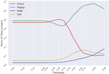
Figure 1: Determining threshold confidence for dataset construction.

An appropriate threshold value needs to be chosen, leading to a good trade-off between high confidence and the appropriate size & distribution of the dataset. The distribution of each class at a threshold approaching $1$ is very different compared to when all samples are taken at the $0$ thresholds. Till the threshold value of $0.33$, the distribution is almost the same as the original, but this confidence is too low to be acceptable. The next possible value is above $0.5$ but below $0.6$. Between these two values, the distribution of various classes is almost the same, and the confidence is also above $0.5$, which is acceptable. Hence, an average value of $0.55$ is chosen as the threshold confidence value.

3.1.2 Human Evaluation

The MMEmoRec dataset has been evaluated by having 8 people evaluate the data samples. We had two human readers (one male and one female) who spoke out and recorded the text components of the data samples. The evaluators listened to the machine-synthesized speech against the human speech recorded by the human readers and scored the contextual similarity between them on a scale of 0 to 100. The human evaluators also evaluated whether the data samples’ speech, image, and text components agree with the annotated emotion sample. The samples have been picked randomly, and the average of the evaluators’ scores has been reported in Table III where $S_{ss-hs}$ denotes the percentage of evaluators reporting the synthetic speech (ss) to be similar to human speech (hs). $S_{ss}$ & $S_{hs}$ denotes the percentage of speech components of synthetic and human speech portraying the annotated emotion. Likewise, $S_{i}$ and $S_{t}$ denote the agreement of annotated emotion class by image and text components. $S_{ss-i-t}$ and $S_{hs-i-t}$ show the samples showing agreement of the annotated emotion class by all three modalities on considering synthetic and human speech, respectively.

TABLE III: Human evaluation of MMEmoRec dataset.

Class	$S_{ss-hs}$	$S_{ss}$	$S_{hs}$	$S_{i}$	$S_{t}$	$S_{ss-i-t}$	$S_{hs-i-t}$
Angry	67.18%	82.81%	85.94%	70.31%	84.38%	75.00%	82.03%
Happy	52.78%	66.67%	69.44%	63.89%	72.22%	66.67%	69.44%
Hate	62.50%	71.43%	72.32%	67.86%	71.43%	73.21%	72.32%
Sad	60.42%	77.08%	78.13%	75.00%	87.50%	77.08%	83.33%
Overall	60.72%	74.49%	76.46%	69.26%	78.81%	72.99%	76.78%

We had two readers read the text of the data samples and called their output human-synthesized speech. 60.72% evaluators found the synthetic speech to be contextually similar to the human synthesized speech. 74.49% synthetic speech samples and 78.91% human synthesized speech samples were found to portray the annotated emotion labels. As per further observations, 69.26% images and 78.81% text components of the data samples correspond to the annotated emotion labels. Moreover, the evaluators also reported that 72.99% of the samples considering machine-synthesized speech along with the corresponding text & image were in line with the determined emotion label, whereas this is comparable to the value of 76.74% on considering human synthesized speech along with the corresponding text & image.

3.2 VISTA Net

The proposed system, VISTA Net’s architecture, is shown in Fig. 2, which has been decided based on the ablation studies discussed in Section 4.3.1. It fuses image, speech & text features using a hybrid of two-stage intermediate and late fusion, which considers all possible pairs of all three modalities and automatically weights them without human intervention. The intermediate fusion combines the information from various modalities before classifying, i.e., after feature extraction, whereas late fusion combines the information after classification.

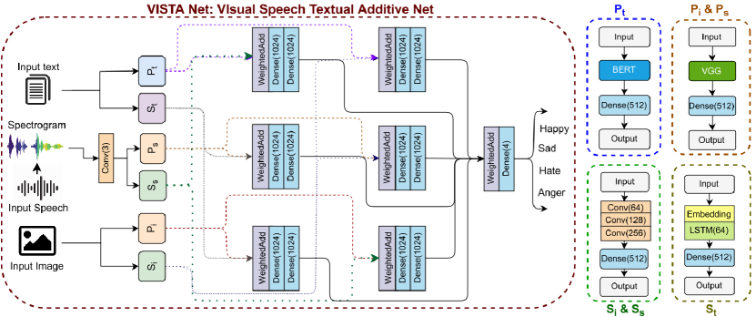
Figure 2: Schematic architecture of the proposed multimodal emotion recognition system. Here, $\mathbf{P_{m}}$ & $\mathbf{S_{m}}$ denote the pre-trained & simpler networks for $m^{th}$ modality whereas ‘i,’ ‘s,’ and ‘t’ denote visual, speech and text modalities, respectively.

The three modalities are fed into two types of networks: a pre-trained and a simpler network. The intuition behind this approach is to build a fully automated multimodal emotion classifier by including various modalities in all possible combinations and learning their weights while training without any human intervention. The proposed system contains $P_{i}$ and $S_{i}$ for image, $P_{s}$ and $S_{s}$ for speech, and $P_{t}$ and $S_{t}$ for text, denoting pre-trained and simpler networks, respectively. The input speech has been converted to a log-mel spectrogram before feeding into the network.

3.2.1 Intermediate Fusion Phase

The images of dimension $(128,\ 128,\ 3)$ are fed into $P_{i}$ and $S_{i}$ respectively, with $P_{i}$ consisting of VGG16 [58] and a $512$-dimensional dense layer and $S_{i}$ containing 3 convolution layers of $64$, $128$ and $256$ filters of size $(3,\ 3)$ and a dense layer of $512$ dimensions. The spectrogram of size $(128,\ 128,\ 1)$ from speech input is passed from a $3$ filter convolution layer of size $(1,\ 1)$, to make it compatible with VGG16. Further, it is passed from $P_{s}$ and $S_{s}$, consisting of the same architecture as $P_{i}$ and $S_{i}$, respectively.

The text input is similarly passed from $T_{i}$ containing a BERT [59] and $T_{s}$ consisting of an embedding and LSTM layer with $64$ units. Both $T_{i}$ & $T_{s}$ are followed by $512$-dimensional dense layers. In the intermediate fusion, all pairs of the pre-trained and simpler networks from different modalities are created by passing them from the $WeightedAdd$ layer we have defined. It gives us six such combinations passed from $2$ dense layers with $1024$ neurons, giving the classification based on each pair. The Eq. 1 shows all the possible pairs formed from the combination of pre-trained and simpler networks such that both the networks do not belong to the same modality.

$$\begin{split}&O_{1}=WeightedAdd(P_{i},S_{s})\\ &O_{2}=WeightedAdd(P_{i},S_{t})\\ &O_{3}=WeightedAdd(P_{s},S_{i})\\ &O_{4}=WeightedAdd(P_{s},S_{t})\\ &O_{5}=WeightedAdd(P_{t},S_{i})\\ &O_{6}=WeightedAdd(P_{t},S_{s})\\ \end{split}$$ (1)

where $O_{1}$, $O_{2}$, $O_{3}$, $O_{4}$, $O_{5}$, and $O_{6}$ are the classification outputs for various pairs of pre-trained and simpler networks. The $WeightedAdd$ layer ensures that during training, the weight of any weighted addition is learned using back-propagation without any human intervention. Each weight in the $WeightedAdd$ layer is randomly initialized and passed from the softmax layer, giving us positive values used as final weights and learned during training.

3.2.2 Late Fusion Phase

In this phase, the information from various modalities’ all possible pairs is combined in a hybrid manner. The intermediate classification outputs obtained from above Eq. 1 are passed from another $WeightedAdd$ layer, which combines these outputs dynamically, giving us the final output $O$ as depicted in Eq. 2. The output $O$ is passed from a dense layer with dimensions equal to the number of emotion classes, i.e., four.

$$O=WeightedAdd(O_{1},O_{2},O_{3},O_{4},O_{5},O_{6})$$ (2)

where $O$ denotes the final output and $O_{1}$, $O_{2}$, $O_{3}$, $O_{4}$, $O_{5}$ and $O_{6}$ are the intermediate classification outputs.

3.3 KAAP

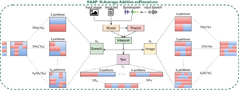
Figure 3: Schematic representation of the proposed interpretability technique. Where $k_{i}$, $k_{s}$, and $k_{t}$ denote the no. of partitions for image, speech, and text modalities; $w_{i}$, and $w_{s}$ are the widths for image & speech feature matrices, and $L_{t}$ is text feature vector’s length.

This Section proposes a novel multimodal interpretability technique, K-Average Additive exPlanation (KAAP), depicted in Fig. 3. It computes the importance of each modality and its features while predicting a particular emotion class. The existing interpretability techniques do not apply to speech and multimodal emotion recognition. Moreover, the most frequently used and accepted interpretability technique for images and text is SHAP [42], which is an approximation of Shapley values [45]. It requires $O(n^{2})$ computational time-complexity, whereas KAAP requires a time of $O(k^{2})$ where $k<=n$ is a given hyper-parameter. Moreover, KAAP applies to multimodal emotion analysis and a single modality or a combination of any two modalities.

Define $model$: DNN model,

Define $img$: Image data,

Define $text$: text data,

Define $speech$: Speech spectrogram data,

Define $type$: The type of data whose perturbed probability is required

procedure Predict ($model,\ img,\ text,\ speech,\ w,\ type$)

if $type==image$ then

       $prob=model.predict\_proba(img,0,0)$

end if

if $type==text$ then

       $prob=model.predict\_proba(0,text,0)$

end if

if $type==speech$ then

       $prob=model.predict\_proba(0,0,speech)$

end if

return $prob$

Algorithm 1 Predict (Probability Prediction)

Define $model$: DNN model, $img$: Image data, $text$: text data, $speech$: Speech spectrogram data,

Define $w$: Size of data; $k$: Parts in which data is divided; $type$: The type of data 

procedure KAAP_helper ($model,\ img,\ text,\ speech,\ w,\ k,\ type$)

$p_{f}=Predict(img,\ text,\ speech,\ type)$;

$p_{b}=Predict(0,\ 0,\ 0,\ type)$;

$kaap=np.zeros(w)$

for $i\leftarrow k$ do

       $parts=make\_parts(w,i)$

      for $j\leftarrow len(parts)$ do

            

            $part=parts[j]$ if $type==image$ then

                   $data\_1=np.zeros(w)$

                   $data\_1[part]=img[part]$

                   $data\_2=img$

                   $data\_2[part]=np.zeros(part)$

             end if

            if $type==text$ then

                   $data\_1=np.zeros(w)$

                   $data\_1[part]=text[part]$

                   $data\_2=text$

                   $data\_2[part]=np.zeros(part)$

             end if

            if $type==speech$ then

                   $data\_1=np.zeros(w)$

                   $data\_1[part]=speech[part]$

                   $data\_2=speech$

                   $data\_2[part]=np.zeros(part)$

             end if

            $p_{1}=Predict(data\_1,\ data\_1,\ data\_1,type)$

             $p_{2}=Predict(data\_2,\ data\_2,\ data\_2,type)$

            $kp\_values=\frac{1}{j}*(p_{1}-p_{b})+\frac{1}{1-j}*(p_{f}-p_{2})$

             if $type==image$ or $type==speech$ then

                   $kaap\mathrel{+}=(\frac{i}{w})^{2}*kp\_values$

             end if

            if $type==text$ then

                   $kaap\mathrel{+}=\frac{i}{w}*kp\_values$

             end if

            

       end for

      

end for

$kaap=\frac{kaap}{sum(kaap)}$

return $kaap$

Algorithm 2 KAAP_helper (Procedure to calculate KAAP value for each data instance)

Define $model$: DNN model,

Define $img$: Image data,

Define $text$: text data,

Define $speech$: Speech spectrogram data,

Define $w$: Width of the input

Define $k$: Parts in which data is divided

Define $type$: The type of data KAAP values are required 

procedure KAAP ($model,\ img,\ text,\ speech,\ w,\ k,\ type$)

$p_{f}=model.predict\_proba(img,\ text,\ speech)$

$p_{b}=model.predict\_proba(0,\ 0,\ 0)$

$p_{i1}=model.predict\_proba(img,\ 0,\ 0)$

$p_{i2}=model.predict\_proba(0,\ text,\ speech)$

$s\_i=\frac{1}{3}*(p_{i1}-p_{b})+\frac{2}{3}*(p_{f}-p_{i2})$

$kaap\_img=KAAP\_helper\hfill(model,\ img,\ text,\ speech,\ w,\ k,\ image)$

$p_{t1}=model.predict\_proba(0,\ text,\ 0)$

$p_{t2}=model.predict\_proba(img,\ 0,\ speech)$

$s\_t=\frac{1}{3}*(p_{t1}-p_{b})+\frac{2}{3}*(p_{f}-p_{t2})$

$kaap\_text=KAAP\_helper\hfill(model,\ img,\ text,\ speech,\ w,\ k,\ text)$

$p_{s1}=model.predict\_proba(0,\ 0,\ speech)$

$p_{s2}=model.predict\_proba(img,\ text,\ 0)$

$s\_s=\frac{1}{3}*(p_{s1}-p_{b})+\frac{2}{3}*(p_{f}-p_{s2})$

$kaap\_speech=KAAP\_helper\hfill(model,\ img,\ text,\ speech,\ w,\ k,\ speech)$

return $(s\_i,\ s\_t,\ s\_s,\ kaap\_img,\ kaap\_text,\ kaap\_speech)$

Algorithm 3 KAAP

3.3.1 Calculating K-exPlanable Values

For a model with $k$ features $\{f_{1},f_{2},\dots\ f_{k}\}$, K-exPlanable (KP) value of feature $f_{i}$, $kp_{f_{i}}$ denotes its importance. Fig. 4 depicts an example calculation.

Consider four nodes, Node $1$ with no feature i.e NULL, Node $2$ with a single feature $f_{i}$, Node $3$ with all the remaining features left in Node $1$, i.e. , $\{f_{1},f_{2},\dots,f_{(i-1)},f_{(i+1)},\dots,\ f_{k}\}$, and Node $4$ with all the features $\{f_{1},f_{2},\dots,f_{(i-1)},f_{i},f_{(i+1)},\dots,\ f_{k}\}$. The ‘Marginal Contribution’ of an edge connecting Node $i$ and Node $j$ is defined as the difference between the prediction probabilities on using their features. For a given predicted label $c$, the marginal contribution of the feature $f_{i}$ for the edge from Node $1$ to Node $2$ is calculated using Eq. 3. Here, $prob_{\{f_{i}\}}$ is the probability of label $c$ calculated by having only feature $f_{1}$ in the input and perturbing all other features to zero.

$$\begin{split}&MC_{f_{i},\{f_{i}\}}=prob_{\{f_{i}\}}-prob_{\{\phi\}}\\ \end{split}$$ (3)

To find the overall importance of $f_{i}$, we calculate the weighted average of all ‘marginal contribution’ of $f_{i}$ given by Eq. 3.3.1.

$$KP_{\{f_{i}\}}(k) =w_{12}\times MC_{f_{i},\{f_{i}\}}$$

$$\quad+w_{34}\times MC_{f_{i},\{f_{1},\ f_{2},\ \dots,f_{k}\}}$$ (4)

where $w_{12}$ and $w_{34}$ are the weights for the weighted addition. Now, there are two conditions on the weights: i) the sum of weights equals one; this is done to normalize the weights; ii) the weight $w_{34}$ must be $(k-1)$ times the weight $w_{12}$. The second condition is based on the fact that $MC_{f_{i},\{f_{i}\}}$ is the effect of addition of $f_{i}$ in an empty set of features, while $MC_{f_{i},\{f_{1},f_{2},\dots,f_{k}\}}$ is the effect of addition on a set containing $(k-1)$ features. It results in Eq. 5.

$$w_{12}+w_{34}=1;\hskip 14.45377ptw_{12}=\frac{w_{34}}{k-1}$$ (5)

where the values of $w_{12}$ and $w_{34}$, shown in Eq. 6 are computed using Eq. 5.

$$w_{12}=\frac{1}{k};\hskip 14.45377ptw_{34}=1-\frac{1}{k}$$ (6)

The KP values shown in Eq. 7 are computed using Eq. 3.3.1 and Eq. 6.

$$KP_{\{f_{i}\}}(k)=\frac{1}{k}\times MC_{f_{i},\{f_{i}\}}+(1-\frac{1}{k})\times MC_{f_{i},\{f_{1},f_{2},\dots,f_{k}\}}$$ (7)

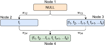
Figure 4: Sample model for KP values computation.

3.3.2 Calculating KAAP Values

This Section computes the KAAP values and uses them to determine the importance of each modality and its features. The information of image, text, and speech modalities are in the same data format, i.e., continuous format. A single pixel can not define an object that can lead to a particular emotion for an image, but a group of pixels will. For speech, the spectrogram at a single instance of time & frequency alone can not define anything, but a time interval will. Likewise, for text, a single letter may not define an emotion, but a word can do so. KAAP values have been defined based on the motivation from the aforementioned fact. They are computed using the KP values for a group of features.

First, the input of size $l$ is divided into $k$ parts, where $k$ is a hyperparameter decided through the ablation study in Section 4.3. These $k$ parts correspond to the $k$ features of the input. Then, for a feature group $f_{i}$, $KP_{f_{i}}(k)$ values are computed for the given value of $k$ using Eq 6. It represents how a group of features $f_{i}$ will perform compared to all remaining groups. However, these groups can vary in size, i.e., $k$ can have various values that lead to different groups and thus to different KP values from groups of different sizes, thus affecting the original features’ importance. To deal with this issue, the weighted average of all the KP values is taken for $k\in\{2,3\dotsc,k\}$ where weights are equal to the number of features in that group of features, given by the Eq. 8. It should be noted that $k$ = 1 is ignored here, as the whole input as one feature will not make any sense.

$$kaap_{\{f_{i}\}}=\sum_{j=2}^{k}[\frac{j}{l}\times KP_{\{f_{i}\}}(j)]\hfill\triangleright{\color[rgb]{.5,.5,.5}for\ linear\ feature}$$ (8)

For input image and speech spectrogram, both of width $128$ and height $128$, their KP values for a given $k$ are calculated by dividing the input into $k$ parts along both axes. As a matrix defines image and speech spectrogram, this gives us a $k*k$ feature group. The equation for calculating the KAAP values for the above two inputs is given by Eq. 9. It gives us a matrix showing the importance of each pixel for a given image and speech input. This matrix directly represents the importance of the image. At the same time, for speech input, the values are averaged along the frequency axis to reduce the KAAP value matrix to the time axis, hence giving importance to speech at a given time.

$$kaap_{\{f_{i}\}}=\sum_{j=2}^{k}[\frac{j^{2}}{w^{2}}\times KP_{\{f_{i}\}}(j)]\hfill\triangleright{\footnotesize\color[rgb]{.5,.5,.5}for\ matrix\ feature}$$ (9)

For input text, the division is done such that each text word is considered a feature, as the emotion can only be defined by a word, not a single letter, as discussed above. Then, the text is divided into $k$ parts, and as a linear array can represent text, the KAAP values are calculated using Eq. 8. Also, the value of $k$ used for image, speech, and text modalities have been determined as $7$, $7$, and $5$, respectively, in Section 4.3.2. Furthermore, the modalities’ importance defined by symbols $\upsilon$, $\delta$, and $\tau$ for visual, spoken, and textual features, respectively, are computed assuming that image, speech, and text are three distinct features and calculating each modality’s KAAP value for $k$ = $3$. While finding the importance of the features of a particular modality, all the other modalities are perturbed to zero. The KAAP technique is depicted in Algorithm 3, which uses Algorithm 2 that calculates the KAAP values for each data instance and Algorithm 1 for probability prediction.

4 Implementation

4.1 Experimental Setup

The network training for the proposed system has been carried out on Nvidia Quadro P5000 GPU, whereas the testing & evaluation have been done on an Intel(R) Core(TM) i7-8700 Ubuntu machine with 64-bit OS and 3.70 GHz, 16GB RAM.

4.2 Training Strategy and Hyperparameter Setting

The model training has been performed using a batch-size of $64$, the train-test split of $80$-$20$, Adam optimizer, ReLU activation function with a learning rate of $1\times 10^{-4}$ and ReduceLROnPlateau learning rate scheduler with patience value of $2$. The baselines and proposed models converged in terms of validation loss in $10$ to $15$ epochs. As a safe upper bound, the models have been trained for $50$ epochs with EarlyStopping [60] with patience values of $5$. The loss function is the average of categorical focal loss [61] and categorical cross-entropy loss. Accuracy, macro f1 [62], and CohenKappa [63] have been analyzed for the model evaluation.

4.3 Ablation Studies and Models

The ablation studies have been performed to determine the threshold confidence value for data construction, appropriate network configuration for VISTA Net, and suitable $k$ values for KAAP.

4.3.1 Ablation Study 1: Determining Baselines and Proposed System’s Architecture

To begin with, the emotion recognition has been performed for a single modality at a time, i.e., separate IER, SER, and TER using pre-trained VGG models [58] for Image & speech and BERT [59] for text. The performance has been evaluated in terms of Accuracy, CohenKappa metric (CK), F1 score, Precision, and Recall and summarized in Table IV. The CK metric measures whether the distribution of the predicted class is in line with the ground truth or not.

TABLE IV: Ablation Study 1. ‘Acc,’ ‘F1,’ ‘CK,’ ‘P,’ and ‘R’ denote accuracy, F1-score, CohenKappa score, precision and recall.

Model	Acc	F1	CK	P	R
Image only	60.44	0.60	0.324	0.60	0.60
Speech only	78.69	0.75	0.624	0.74	0.79
Text only	81.51	0.81	0.69	0.81	0.82
Image + Text	86.40	0.86	0.77	0.86	0.86
Image + Speech	84.66	0.85	0.746	0.85	0.85
Text + Speech	81.95	0.81	0.70	0.82	0.81
Image + Speech + Text	86.60	0.86	0.78	0.86	0.87

Next, we moved on to the combination of two modalities. The chosen two modalities are fed into respective pre-trained models and then passed from a dense layer of $512$ neurons. Then the information from these modalities is added using the $WeightedAdd$ layer defined in 3.2.1. This output is next passed from three dense layers of size $1024$, $1024$, and $4$ neurons, which then classifies the emotion.

Finally, the information from all three modalities is combined and fed into their respective pre-trained models and is then passed from a dense layer of size $512$, which is then passed from a $WeightedAdd$ layer; the output of this layer is passed from $3$ dense layers as in the combination of two modalities. Combining all three modalities has performed better than the remaining models in all the evaluation metrics. As observed during the experiments above, combining the information from the complementary modalities has led to better emotion recognition performance. Hence, the baselines and proposed model have been formulated, including all three modalities and various information fusion mechanisms in Section 4.4.

4.3.2 Ablation Study 2: Determining $k$ Values for KAAP

An in-depth ablation study has been conducted here to decide the value of $k$ used in Section 3.3.2. The dice coefficient [64] is used to determine the best $k$ values. It measures the similarity of two data samples; the value of $1$ denotes that the two compared data samples are completely similar, whereas a value of $0$ denotes their complete dis-similarity. For each modality, KAAP values are calculated at $k\in\{2,3\dotsc,10\}$. The dice coefficient is calculated for two adjacent $k$ values. For example, at $k=3$, the KAAP values at $k=2$ and $k=3$ are used to calculate the dice coefficient. The procedure mentioned above has been performed for all three modalities, and the results are visualized in Fig. 5.

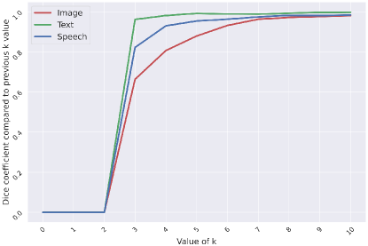
Figure 5: Ablation Study 2: Determining appropriate $k$ values.

The effect of increasing $k$ values can be observed in the figure. For image & speech, the value converges to $1$ at $k$ = 7, while for text, the optimal value of k is $5$.

4.4 Baselines and Proposed Models

The ‘Image + Speech + Text’ configuration described in Section 4.3.1 is considered as baseline 1, whereas further baseline models’ architectures have been formulated by incorporating further improvements in the information fusion mechanisms.

The baseline models are made on a common idea, as described below. Firstly, all three modalities are fed into $P_{i}$, $P_{s}$, $S_{i}$, $S_{s}$, $T_{i}$ and $T_{s}$ as described in Section 3.2, and are then passed from a dense layer of $512$ neurons, resulting in a $512$-dimensional outputs which are then combined using $WeightedAdd$ to give three outputs. The following strategy is being followed for combining them: any pre-trained network must be combined with another simpler network. At least one combination must contain the network from different modalities because if all the modalities combine with themselves, then such a combination will not lead to any information exchange. Thus, six such configurations are possible, as described in Eq. 10.

$$\begin{split}&(\#1):{\{P_{i}+S_{i},P_{s}+S_{s},P_{t}+S_{t}}\}\\ &(\#2):{\{P_{i}+S_{i},P_{s}+S_{t},P_{t}+S_{s}}\}\\ &(\#3):{\{P_{i}+S_{s},P_{s}+S_{i},P_{t}+S_{t}}\}\\ &(\#4):{\{P_{i}+S_{s},P_{s}+S_{t},P_{t}+S_{i}}\}\\ &(\#5):{\{P_{i}+S_{t},P_{s}+S_{i},P_{t}+S_{s}}\}\\ &(\#6):{\{P_{i}+S_{t},P_{s}+S_{s},P_{t}+S_{i}}\}\\ \end{split}$$ (10)

The configuration $(\#1)$ is discarded as it does not hold the condition that at least one combination must combine with a different modality. The configurations $(\#2)$, $(\#3)$, $(\#6)$ are partially-complete combinations as one of the three outputs of these combinations combine the pre-trained and simpler network from the same modalities. On the other hand, the configurations $(\#4)$ and $(\#5)$ are complete.

Using the above strategy puts us in two disadvantages: i) only two out of five such baselines are complete while others are partially complete; ii) different datasets have different requirements. For example, a particular multimodal dataset may have better image and speech components, while other datasets may have a better-quality of text components. To generalize for any dataset and scenario, an automated multimodal emotion recognition system, VISTA Net, has been proposed, which combines all output of baselines 2-6, leaving any self-combination and taking the weighted average of remaining all. Hence, it automatically decides the weights of each combination according to the requirements of problem statements and the dataset. The results for baselines and the proposed system are summarized in the following Section.

5 Results and Discussion

5.1 Quantitative Results

The VISTA Net has achieved emotion recognition accuracy of 95.99%. Its class-wise accuracies are shown in Fig. 6 while its results, along with the results of baselines, are shown in Table V.

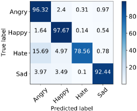
Figure 6: Confusion matrix showing class-wise accuracies.

TABLE V: Results comparison for emotion recognition on IIT-R MMEmoRec dataset. ‘Acc,’ ‘F1,’ ‘CK,’ ‘P,’ & ‘R’ denote accuracy, F1-score, CohenKappa score, precision & recall. Baseline 1 has (Image + Speech + Text) configuration from Section 4.3.1.

Model	Acc	F1	CK	P	R
Baseline 1	86.60	0.86	0.78	0.86	0.87
Baseline 2(#2)	94.89	0.95	0.91	0.95	0.95
Baseline 3(#3)	95.44	0.95	0.92	0.93	0.95
Baseline 4(#4)	95.39	0.95	0.92	0.95	0.95
Baseline 5(#5)	95.58	0.96	0.92	0.96	0.96
Baseline 6(#6)	95.37	0.95	0.92	0.95	0.95
VISTA Net	95.99	0.96	0.93	0.96	0.96

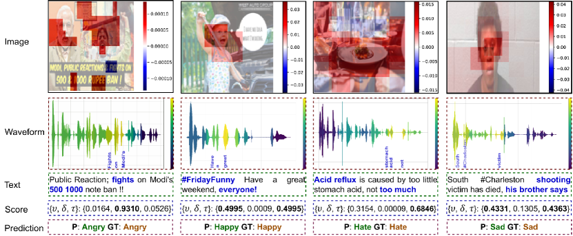
Figure 7: Sample results; here, ‘P,’ ‘GT’ are the predicted and ground-truth labels whereas‘Score’ denotes the importance of visual ($\upsilon$), spoken ($\delta$) & textual ($\tau$) modalities.

5.2 Qualitative Results

Sample emotion classification & interpretation results are shown in Fig. 7. The important speech and image features contributing to emotion classification are obtained, and corresponding words are highlighted. In the waveform, yellow and blue correspond to the most and least important features, respectively. The speech and text were observed to be the most contributing modalities for the prediction of ‘angry’ and ‘hate’ classes, whereas image and text modalities contributed equally to the determination of ‘happy’ and ‘sad’ classes.

5.3 Results Comparison

The emotion recognition results have been reported in Section 5.1. The IIT-R MMEmoRec dataset has been constructed from the B-T4SA dataset in this paper; hence, there are no existing emotion recognition results for it. However, sentiment classification (into ‘neutral,’ ‘negative,’ and ‘positive’ classes) results on the B-T4SA dataset are available in the literature, which have been compared with VISTA Net’s sentiment classification results in Table VI.

TABLE VI: Results comparison for sentiment classification on BT4SA dataset with existing approaches. Here, ‘V,’ ‘S,’ and ‘T’ denote visual, spoken and textual modalities.

Approach	Modality	Accuracy
Cross-Modal Learning [11]	V + T	51.30%
Multimodal Sentiment Analysis [10]	V + T	60.42%
Hybrid Fusion [65]	V + T	86.70%
Automated ML [66]	V + T	95.19%
VISTA Net (Sentiment Classification)	V + S + T	96.59%

5.4 Performance for Missing Modalities

In real-life scenarios, some data samples in the multimodal data may be missing information about one of the modalities. The VISTA Net has been evaluated for such scenarios. We formulated four use cases with image, speech, text, or no modality missing and divided the test dataset into randomly selected equal parts accordingly. Then the information of the missing modality has been overridden to null, and VISTA Net has been evaluated for emotion recognition.

TABLE VII: Results for missing modalities. Here, ‘Acc,’ ‘F1,’ ‘CK,’ ‘P,’ and ‘R’ denote accuracy, F1-score, CohenKappa score, precision and recall.

Model	Acc	F1	CK	P	R
Missing Image	82.59	0.82	0.77	0.86	0.83
Missing Speech	57.62	0.45	0.75	0.75	0.58
Missing Text	62.82	0.68	0.70	0.87	0.63
Missing None	95.90	0.96	0.92	0.96	0.96

Table VII summarizes the results. The emotion recognition performance for Missing no modality (i.e., having the information from all three modalities) aligns with the results observed in Section5.2. Further, missing image modality information has caused the least dip in the performance. Moreover, the information from speech and text modalities combined has resulted in an emotion classification accuracy of 82.59%, whereas including all the modalities resulted in 95.90% accuracy. The aforementioned observations align with the observations in Section 4.3.1 where IER performance was lesser than TER and SER performance.

5.5 Discussion

Various research tasks may require a particular modality’s information more than the others. For example, text and visual information may be secondary for multimodal speech recognition. Similarly, a multimodal emotion dataset might contain better quality information for one modality over others. Typically, human intervention would be needed to decide the importance of each modality. However, the VISTA Net can determine this automatically, considering all possible combinations of modality information and weighing them accordingly.

As the proposed MMEmoRec dataset contains information from complementary modalities, it enables deep learning models to learn the contextually related representation of the underlying emotions. The final label, considered the ground truth of the dataset, is derived by averaging the probabilities of each emotion obtained from unimodal models. Using the same unimodal models for dataset construction can introduce slight bias in performance, but no bias arises when developing and using a new multimodal emotion recognition model. Human evaluators also assessed the IIT-R MMEmoRec dataset for consistency in the determined emotion labels and the appropriateness of the synthesized speech component via text-to-speech.

The experimental results confirm the significance of using information from complementary modalities. As depicted in Fig. 7, different modalities play a crucial role in identifying the overall emotion conveyed by the input data. Some data samples might lack information from a specific modality. The proposed VISTA Net system was tested in such scenarios, and the findings align with the insights from ablation studies.

The proposed interpretability technique, KAAP, computes the importance of each modality and the importance of their respective features towards the prediction of a particular emotion class. The existing interpretability techniques, such as SHAP and LIME, are not applicable to speech modalities, whereas KAAP is applicable to all image, text, and speech modalities. The proposed technique is expected to pave the way for growth in multimedia emotion analysis. We also hope the IIT-R MMEmoRec dataset will inspire further advancements in this context.

6 Conclusions and future work

The proposed system, VISTA Net, performs emotion recognition by considering the information from image, speech & text modalities. It combines the information from these modalities in a hybrid manner of intermediate and late fusion and determines their weights automatically. It has resulted in better performance on including image, speech & text modalities than including only one or two of these modalities. The proposed interpretability technique, KAAP, identifies each modality’s contribution and important features toward predicting a particular emotion class. The future research plan includes transforming emotional content from one modality to another. We will also work on controllable emotion generation, where the output contains the desired emotional tone.

Puneet Kumar (Member, IEEE) received his B.E. and M.E. degrees in Computer Science in 2014 and 2018, respectively, and his Ph.D. from the Indian Institute of Technology Roorkee, India in 2022. He has worked at Oracle Corporation, Samsung R&D, and PaiByTwo Pvt. Ltd., and is now a Postdoctoral Researcher at the University of Oulu, Finland. His research interests include Affective Computing, Multimodal and Interpretable AI, Mental Health, and Computational Cognitive Neuroscience. He has published in top journals and conferences and received various awards, including the institute medal in M.E., the best thesis award, and several best paper awards. For more information, visit his webpage at www.puneetkumar.com.

Sarthak Malik received his B.Tech degree in Electrical Engineering from the Indian Institute of Technology Roorkee, India. He is currently a Data Scientist at MasterCard. He is an avid programmer and an active participant in coding competitions and development projects. His research focuses on Affective Computing, Computer Vision, and Interpetable AI. He has published in reputed journals and conferences and achieved notable recognitions, including a rank in the top 10 in the Geoffrey Hinton Fellowship hackathon. For more details, visit his webpage at www.linkedin.com/in/sarthak-malik.

Balasubramanian Raman (Senior Member, IEEE) received his B.Sc. and M.Sc. degrees from the University of Madras in 1994 and 1996, respectively, and his Ph.D. from the Indian Institute of Technology Madras, India in 2001. He is a Chair Professor in the Department of Computer Science and Engineering and a Joint Faculty in the Mehta Family School of Data Science and Artificial Intelligence at the Indian Institute of Technology Roorkee, India. He has published over 200 research papers in reputed journals and conferences. His research interests include Machine Learning, Image and Video Processing, Medical Imaging, Computer Vision, Activity Recognition, Pattern Recognition, Privacy-Preserving Computing, Data Security. For more information, visit his webpage at http://faculty.iitr.ac.in/cs/bala.

Xiaobai Li (Senior Member, IEEE) received her B.Sc. and M.Sc. degrees in 2004 and 2007, respectively, and her Ph.D. from the University of Oulu, Finland, in 2017. She is currently a ZJU100 professor with the School of Cyber Science and Technology, Zhejiang University, and she is also an Adjunct Professor with the Center for Machine Vision and Signal Analysis, University of Oulu. Her research focuses on Affective Computing, Facial Expression Recognition, Micro-Expression Analysis, Remote Physiological Signal Measurement, and Healthcare. She co-chaired several international workshops in CVPR, ICCV, FG, and ACM Multimedia and is an Associate Editor of IEEE Transactions on Circuits and Systems for Video Technology, Frontiers in Psychology, and Image and Vision Computing. For more information, visit her webpage at www.oulu.fi/en/researchers/xiaobai-li.

References

- [1] T. Baltrušaitis, C. Ahuja et al., “Multimodal Machine Learning: A Survey and Taxonomy,” IEEE Transactions on Pattern Analysis and Machine Intelligence, vol. 41, no. 2, pp. 423–443, 2018.
- [2] K. Ezzameli and H. Mahersia, “Emotion Recognition from Unimodal to Multimodal Analysis: A Review,” Information Fusion, p. 101847, 2023.
- [3] M. Muszynski, L. Tian et al., “Recognizing Induced Emotions of Movie Audiences from Multimodal Information,” IEEE Transactions on Affective Computing, vol. 12, no. 1, pp. 36–52, 2019.
- [4] Y. Wang, H. Yu, W. Gao, Y. Xia, and C. Nduka, “MGEED: A Multimodal Genuine Emotion and Expression Detection Database,” IEEE Transactions on Affective Computing, 2023.
- [5] K. Shingjergji, D. Iren et al., “Interpretable Explainability in Facial Emotion Recognition and Gamification for Data Collection,” in The IEEE International Conference on Affective Computing and Intelligent Interaction (ACII), 2022, pp. 1–8.
- [6] M. Palash and B. Bhargava, “EMERSK–Explainable Multimodal Emotion Recognition with Situational Knowledge,” IEEE Transactions on Multimedia, vol. 1, no. 1, 2023.
- [7] N. Majumder, S. Poria et al., “DialogueRNN: An Attentive RNN for Emotion Detection in Conversations,” in The 31st AAAI Conference on Artificial Intelligence (AAAI), vol. 33, no. 01, 2019, pp. 6818–6825.
- [8] S. Malik, P. Kumar, and B. Raman, “Towards Interpretable Facial Emotion Recognition,” in The 12th Indian Conference on Computer Vision, Graphics and Image Processing (ICVGIP), 2021, pp. 1–9.
- [9] C. Busso et al., “IEMOCAP: Interactive Emotional dyadic MOtion CAPture data,” Language Resources & Evaluation, vol. 42, no. 4, 2008.
- [10] A. Gaspar and L. A. Alexandre, “A Multimodal Approach to Image Sentiment Analysis,” in Springer International Conference on Intelligent Data Engineering and Automated Learning (IDEAL), 2019, pp. 302–309.
- [11] L. Vadicamo, F. Carrara et al., “Cross-Media Learning for Image Sentiment Analysis in the Wild,” in IEEE International Conference on Computer Vision Workshops (ICCV-W), 2017, pp. 308–317.
- [12] E. Jing, Y. Liu et al., “A deep Interpretable Representation Learning Method for Speech Emotion Recognition,” Information Processing & Management, vol. 60, no. 6, p. 103501, 2023.
- [13] J. Lorenzo-Trueba, R. Barra-Chicote et al., “Emotion Transplantation Through Adaptation in HMM-based Speech Synthesis,” Computer Speech & Language, vol. 34, no. 1, pp. 292–307, 2015.
- [14] R. Udendhran, M. Garg, and A. K. Yadav, “Explainable Convolutional Neural Network with Facial Emotion Enabled Music Recommender System,” in 4th International Conference on Information Management and Machine Intelligence (ICIMMI), 2022.
- [15] D. Dai, Z. Wu et al., “Learning Discriminative Features from Spectrograms using Center Loss for SER,” in IEEE International Conference on Acoustics, Speech and Signal Processing (ICASSP), 2019, pp. 7405–7409.
- [16] K. Kim and N. Cho, “Focus-Attention-Enhanced Crossmodal Transformer with Metric Learning for Multimodal Speech Emotion Recognition,” pp. 1–4, 2023.
- [17] Q. Mao, M. Dong et al., “Learning Salient Features for Speech Emotion Recognition using Convolutional Neural Networks,” IEEE Transactions on Multimedia (TMM), vol. 16, no. 8, pp. 2203–2213, 2014.
- [18] H. Ma, J. Wang, H. Lin, B. Zhang, Y. Zhang, and B. Xu, “A Transformer-based Model with Self-Distillation for Multimodal Emotion Recognition in Conversations,” IEEE Transactions on Multimedia, 2023.
- [19] J. Li, X. Wang et al., “GA2MIF: Graph and Attention based Two-Stage Multi-Source Information Fusion for Conversational Emotion Detection,” IEEE Transactions on Affective Computing, 2023.
- [20] A. M. Abubakar, D. Gupta, and S. Palaniswamy, “Explainable Emotion Recognition from Tweets using Deep Learning and Word Embedding Models,” in IEEE 19th India Council International Conference (INDICON), 2022, pp. 1–6.
- [21] M. Firdaus, H. Chauhan, A. Ekbal, and P. Bhattacharyya, “EmoSen: Generating Sentiment and Emotion Controlled Responses in a Multimodal Dialogue System,” IEEE Transactions on Affective Computing, vol. 13, no. 3, pp. 1555–1566, 2020.
- [22] J. Li, X. Wang et al., “GraphCFC: A Directed Graph based Cross-Modal Feature Complementation Approach for Multimodal Conversational Emotion Recognition,” IEEE Transactions on Multimedia, 2023.
- [23] K. Shrivastava, S. Kumar, and D. K. Jain, “An Effective Approach for Emotion Detection in Multimedia Text Data using Sequence based Convolutional Neural Network,” Multimedia Tools and Applications, vol. 78, no. 20, pp. 29 607–29 639, 2019.
- [24] E. Batbaatar, M. Li, and K. H. Ryu, “Semantic Emotion Neural Network for Emotion Recognition from Text,” IEEE Access, vol. 7, pp. 111 866–111 878, 2019.
- [25] C. A. Corneanu, M. O. Simón et al., “Survey on RGB, 3D, Thermal, and Multimodal Approaches for Facial Expression Recognition: History, Trends, and Affect-Related Applications,” IEEE Transactions on Pattern Analysis and Machine Intelligence, vol. 38, no. 8, pp. 1548–1568, 2016.
- [26] P. Bhattacharya, R. K. Gupta, and Y. Yang, “Exploring the Contextual Factors Affecting Multimodal Emotion Recognition in Videos,” IEEE Transactions on Affective Computing, 2021.
- [27] A. R. Asokan, N. Kumar, A. V. Ragam, and S. Shylaja, “Interpretability for Multimodal Emotion Recognition using Concept Activation Vectors,” in International Joint Conference on Neural Networks (IJCNN). IEEE, 2022, pp. 01–08.
- [28] M. R. Makiuchi, K. Uto, and K. Shinoda, “Multimodal Emotion Recognition with High-level Speech and Text Features,” in IEEE Automatic Speech Recognition and Understanding Workshop (ASRU), 2021.
- [29] S. Yoon, S. Byun, and K. Jung, “Multimodal Speech Emotion Recognition using Audio and Text,” in IEEE Spoken Language Technology Workshop (SLT), 2018, pp. 112–118.
- [30] P. Kumar, V. Kaushik et al., “Towards the Explainability of Multimodal Speech Emotion Recognition,” in INTERSPEECH, 2021, pp. 1748–1752.
- [31] S. Siriwardhana, A. Reis, and R. Weerasekera, “Jointly Fine Tuning ‘BERT-Like’ Self Supervised Models to Improve Multimodal Speech Emotion Recognition,” INTERSPEECH, pp. 3755–3759, 2020.
- [32] T. Zhu, L. Li, J. Yang, S. Zhao, and X. Xiao, “Multimodal Emotion Classification with Multi-Level Semantic Reasoning Network,” IEEE Transactions on Multimedia, 2022.
- [33] J. Xie, J. Wang et al., “A Multimodal Fusion Emotion Recognition Method based on Multitask Learning and Attention Mechanism,” Neurocomputing, vol. 556, p. 126649, 2023.
- [34] N. Xu, W. Mao, and G. Chen, “A Co-memory Network for Multimodal Sentiment Analysis,” in ACM International Conference on Research & Development in Information Retrieva (SIGIR), 2018.
- [35] D. Nguyen, D. T. Nguyen et al., “Deep Auto-Encoders with Sequential Learning for Multimodal Dimensional Emotion Recognition,” IEEE Transactions on Multimedia, vol. 24, pp. 1313–1324, 2021.
- [36] P. Kumar, S. Malik, and B. Raman, “Interpretable Multimodal Emotion Recognition Using Hybrid Fusion of Speech and Image Data,” Multimedia Tools and Applications, pp. 1–22, 2023.
- [37] Y. Aytar, C. Vondrick, and A. Torralba, “SoundNet: Learning Sound Representations from Ulabeled Video,” in Advances in neural information processing systems (NeurIPS), 2016, pp. 892–900.
- [38] C. Guanghui and Z. Xiaoping, “Multimodal Emotion Recognition by Fusing Correlation Features of Speech-Visual,” IEEE Signal Processing Letters, vol. 28, pp. 533–537, 2021.
- [39] S. Zhang, Y. Yang et al., “Deep Learning-based Multimodal Emotion Recognition from Audio, Visual, and Text Modalities: A Systematic Review of Recent Advancements and Future Prospects,” Expert Systems with Applications, p. 121692, 2023.
- [40] S. Poria, E. Cambria et al., “Fusing Audio, Visual and Textual Clues for Sentiment Analysis from Multimodal Content,” Neurocomputing, vol. 174, pp. 50–59, 2016.
- [41] P. Tzirakis, G. Trigeorgis et al., “End-to-End Multimodal Emotion Recognition Using Deep Neural networks,” IEEE Journal of Selected Topics in Signal Processing, vol. 11, no. 8, pp. 1301–1309, 2017.
- [42] S. M. Lundberg and S.-I. Lee, “A Unified Approach to Interpreting Model Predictions,” in The 31st International Conference on Neural Information Processing Systems (NeurIPS), 2017, pp. 4768–4777.
- [43] M. B. Fazi, “Beyond Human: Deep Learning, Explainability and Representation,” Theory, Culture & Society, 2020.
- [44] A. Shrikumar, P. Greenside, and A. Kundaje, “Learning Important Features Through Propagating Activation Differences,” in International Conference on Machine Learning (ICML), 2017, pp. 3145–3153.
- [45] L. Shapley, “A Value for n-person Games, Contributions to the Theory of Games II,” 1953.
- [46] J. Castro et al., “Polynomial calculation of The Shapley Value based on Sampling,” Elsevier Computers & Operations Research, vol. 36, no. 5, pp. 1726–1730, 2009.
- [47] R. Fong, M. Patrick et al., “Understanding Deep Networks Via Extremal Perturbations and Smooth Masks,” in The IEEE/CVF International Conference on Computer Vision (ICCV), 2019, pp. 2950–2958.
- [48] M. T. Ribeiro, S. Singh, and C. Guestrin, “Why Should I Trust You? Explaining Predictions of Any Classifier,” in International Conference on Knowledge Discovery & Data mining (KDD), 2016, pp. 1135–1144.
- [49] K. Simonyan, A. Vedaldi, and A. Zisserman, “Deep Inside Convolutional Networks: Visualising Image Classification Models and Saliency Maps,” in Proceedings of the International Conference on Learning Representations (ICLR), 2014.
- [50] R. R. Selvaraju, M. Cogswell et al., “Grad-CAM: Visual Explanations from Deep Networks via Gradient-based Localization,” in The IEEE/CVF International Conference on Computer Vision (ICCV), 2017, pp. 618–626.
- [51] P.-J. Kindermans et al., “The (Un)reliability of Saliency Methods,” in Explainable AI: Interpreting, Explaining and Visualizing Deep Learning, 2019, pp. 267–280.
- [52] A. Zadeh, P. P. Liang, S. Poria, P. Vij, E. Cambria, and L.-P. Morency, “Multi Attention Recurrent Network for Human Communication Comprehension,” in The AAAI Conference on Artificial Intelligence, 2018.
- [53] W. Ping, K. Peng et al., “DeepVoice 3: Scaling Text-to-Speech with Convolutional Sequence Learning.” in The 6th International Conference on Learning Representations (ICLR), 2018.
- [54] A. v. d. Oord, S. Dieleman et al., “Wavenet: A Generative Model for Raw Audio,” ArXiv Preprint ArXiv:1609.03499, 2016, Accessed 30 Oct 2023.
- [55] Q. You, J. Luo, H. Jin, and J. Yang, “Building a Large Scale Dataset for Image Emotion Recognition: the Fine Print and the Benchmark,” in The AAAI Conference on Artificial Intelligence (AAAI), 2016, pp. 308–314.
- [56] K. R. Scherer and H. G. Wallbott, “Evidence For Universality and Cultural Variation of Differential Emotion Response Patterning.” Journal of Personality and Social Psychology, vol. 66, no. 2, p. 310, 1994.
- [57] R. Plutchik, “The Nature of Emotions,” Journal Storage Digital Library’s American scientist Journal, vol. 89, no. 4, pp. 344–350, 2001.
- [58] K. Simonyan and A. Zisserman, “Very Deep Convolutional Networks for Large-Scale Image Recognition,” Arxiv Preprint ArXiv:1409.1556, 2014, Accessed 30.06.2022.
- [59] J. Devlin, M.-W. Chang, K. Lee, and K. Toutanova, “BERT: Pre-training of Deep Bidirectional Transformers for Language Understanding,” ArXiv Preprint ArXiv:1810.04805, 2018, Accessed 30 Oct 2023.
- [60] L. Prechelt, “Early Stopping - But When?” in Neural Networks: Tricks of the trade. Springer, 1998, pp. 55–69.
- [61] T.-Y. Lin, P. Goyal et al., “Focal Loss for Dense Object Detection,” in Proceedings of the IEEE/CVF Conference on Computer Vision (ICCV), 2017, pp. 2980–2988.
- [62] J. Opitz and S. Burst, “Macro F1 and Macro F1,” ArXiv Preprint ArXiv:1911.03347, 2019, Accessed 30 Oct 2023.
- [63] S. M. Vieira, U. Kaymak, and J. M. Sousa, “Cohen’s Kappa Coefficient as a Performance Measure for Feature Selection,” in The 18th IEEE International Conference on Fuzzy Systems (IEEE-FUZZ), 2010, pp. 1–8.
- [64] R. Deng, C. Shen, S. Liu, H. Wang, and X. Liu, “Learning to Predict Crisp Boundaries,” in The European Conference on Computer Vision (ECCV), 2018, pp. 562–578.
- [65] P. Kumar, V. Khokher, Y. Gupta, and B. Raman, “Hybrid Fusion based Approach for Multimodal Emotion Recognition with Insufficient Labeled Data,” in The 28th IEEE International Conference on Image Processing (ICIP), 2021, pp. 314–318.
- [66] V. Lopes, A. Gaspar, L. A. Alexandre, and J. Cordeiro, “An AutoML-based Approach to Multimodal Image Sentiment Analysis,” in The International Joint Conference on Neural Networks (IJCNN). IEEE, 2021, pp. 1–9.