Towards a Lower Bound for the Average Case Runtime of Simulated Annealing on TSP

Abstract

We analyze simulated annealing (SA) for simple randomized instances of the Traveling Salesperson Problem. Our analysis shows that the theoretically optimal cooling schedule of Hajek [16] explores members of the solution set which are in expectation far from the global optimum. We obtain a lower bound on the expected length of the final tour obtained by SA on these random instances. In addition, we also obtain an upper bound on the expected value of its variance. These bounds assume that the Markov chain that describes SA is stationary, a situation that does not truly hold in practice. Hence, we also formulate conditions under which the bounds extend to the nonstationary case. These bounds are obtained by comparing the tour length distribution to a related distribution. We furthermore provide numerical evidence for a stochastic dominance relation that appears to exist between these two distributions, and formulate a conjecture in this direction. If proved, this conjecture implies that SA stays far from the global optimum with high probability when executed for any sub-exponential number of iterations. This would show that SA requires at least exponentially many iterations to reach a global optimum with nonvanishing probability.

1 Introduction

Discrete minimization problems require one to minimize an objective function over a finite set of solutions. In many cases of interest, the computational effort required to find a globally optimal solution is assumed to be prohibitively large. A classical example is the Traveling Salesperson Problem (TSP): given a weighted graph $G$, the goal is to find a minimum-weight Hamiltonian cycle of $G$. Although easily stated, the TSP is NP-hard [20].

To nevertheless obtain solutions that are satisfactory, a common resolution is to apply local search heuristics rather than exact algorithms. Although these heuristics are not guaranteed to converge to the global optimum, they often find solutions of surprisingly high quality. Moreover, the problem of finding local optima appears to be tractable on practical instances, despite the pessimistic worst case performance of many of these heuristics [31, 4, 11, 7]. In particular, the $k$-opt heuristic for TSP gives near-optimal solutions for Euclidean instances [8], and runs in polynomial time in practice, as demonstrated in a study by Johnson & McGeoch [2, chapter 8].

While local improvement heuristics are quite successful, they are prone to getting stuck in local optima. An approach to solving this problem can be found in metaheuristics such as simulated annealing (SA) [1, 15]. At the basis of SA lies a local improvement heuristic. However, rather than requiring every step of the optimization process to strictly decrease the objective function, a probabilistic approach is taken wherein the objective function is allowed to increase. As such, SA can escape a local optimum in which a local improvement heuristic would get stuck.

To control the probability with which these increasing steps are taken, a control parameter called the temperature is used. At low temperatures, the probability of increasing the objective function should become small; indeed, SA is effectively identical to its underlying local search heuristic at a temperature of 0. Previous results [12, 16] show that for sufficiently slowly decreasing temperature, simulated annealing asymptotically converges to the global optimum. Even at a finite temperature, one can show that the global optimum is eventually reached with high probability [26].

Unfortunately, while rigorous, these bounds are not practically useful. In the case of the TSP, they can only guarantee convergence within $O(n^{n})$ steps [1, 26], which is more costly than even a complete enumeration of the search space. In practice, the algorithm is thus terminated long before convergence is guaranteed.

These upper bounds are furthermore taken with respect to all instances, and thus can be considered worst-case bounds. As the typical runtime of local search heuristics is often much better than the worst case runtime, a natural question to ask is then if we can prove a better bound for simulated annealing on average-case instances.

Here, we set out towards a rigorous lower bound on the expected time to reach the optimal TSP tour for a simple class of random TSP instances. These results are formally stated in Section 2.3. We prove a lower bound on the expected value of the tour length obtained by the algorithm if the underlying Markov chain is assumed to be in equilibrium. Furthermore, we show that this bound also holds out of equilibrium, assuming the Markov chain is sufficiently mixed. Finally, we formulate a conjecture on the statistical behavior of the tour length. Proving this conjecture would allow us to obtain a rigorous lower bound on the runtime of simulated annealing for the logarithmic cooling schedule derived by Hajek [16].

2 Preliminaries

2.1 Notation and Definitions

Throughout the paper, we use $\mathbb{R}_{+}$ to refer to the nonnegative reals, and $\mathbb{R}_{++}$ for the positive reals.

Consider any discrete minimization problem with finite solution space $S$ and associated objective function $J:S\to\mathbb{R}_{+}$. We denote by $n\in\mathbb{N}$ the problem size, which is simply the number of nodes of the underlying TSP instance in most cases in this paper.

Since simulated annealing defines a Markov chain on $S$, it is convenient to consider the state graph of this Markov chain. To that end, we first define a neighborhood structure on $S$, which is simply a function $N:S\to 2^{S}$. Although the neighborhood function can be arbitrary in principle, it is usually highly structured. The state graph is then given by the directed graph $H=(S,A)$, where we have $(x,y)\in A$ iff $y\in N(x)$.

The neighborhood function is often symmetric, in the sense that if $x\in N(y)$ then $y\in N(x)$. In this case, we will regard the state graph as undirected. This definition of the neighborhood differs from the one usually used in the context of local search, where $x\in N(y)$ only if $J(x)<J(y)$. We relax this requirement here, since simulated annealing may increase the objective function in any given iteration.

In this paper, we will always assume that the neighborhood $N$ is symmetric. In other words, we consider only local search heuristics with reversible iterations. Hence, the state graph $H$ considered here is undirected. In addition, we assume throughout that $H$ is $d$-regular, where $d$ may be a function of $n$. In particular, for the TSP with the 2-opt heuristic, the state graph has $|S|=(n-1)!/2$ and is $n(n-3)/2$-regular.

We call a nonincreasing function $T:\mathbb{N}\to\mathbb{R}_{++}$ a cooling schedule. In the context of the physical process that SA takes its inspiration from, a cooling schedule determines the rate at which the temperature of a material is decreased with time. The choice of the cooling schedule is in principle arbitrary. A trade-off exists between the quality of the solution obtained, and the rate at which $T$ decreases. Slowly decreasing cooling schedules potentially yield optimal solutions [16], but may be impractical [1].

Since SA uses a Markov chain, it is a randomized algorithm. In this work, we will analyze the performance of SA on random instances. Thus, the involved Markov chains and their stationary distributions will be functions of the randomness present in the instances. In order to meaningfully assign probabilities, the formalism of compound distributions is useful.

Suppose $\pi(x\>\lvert\>\theta)$ denotes a probability measure on $S$, dependent on a set of parameters $\theta$. We write $\mathbb{E}_{\pi}(f\>\lvert\>\theta)$ for the conditional expected value of $f:S\to\mathbb{R}$. If $\theta$ are themselves distributed according to $\mu$, we write the unconditional or compound expectation $\mathbb{E}(f)=\mathbb{E}_{\mu}(\mathbb{E}_{\pi}(f\>\lvert\>\theta))$. Moreover, we have the joint distribution $p(x,\theta)=\pi(x\>\lvert\>\theta)\mu(\theta)$, which is the generalization of the mixture distribution [24] to the uncountable setting.

Finally, to avoid ambiguities, we provide a definition of the version of simulated annealing we consider in this paper in Algorithm 1.

Data: Solution space $S$, neighborhood function $N$, cooling schedule $T$, a fixed number of iterations $t\in\mathbb{N}$, and a state $x_{0}\in S$.

for $i\in[t]$ do

       generate a state $y\in N(x_{i})$ uniformly at random;

       $\Delta\leftarrow J(y)-J(x_{i})$;

       if $\Delta<0$ then

             $x_{i+1}\leftarrow y$;

            

      else

             $p\leftarrow\exp\left(-\Delta/T(i)\right)$;

             set $x_{i+1}$ to $y$ with probability $p$ and to $x_{i}$ with probability $1-p$;

            

       end if

      

end for

return $x_{t}$

Algorithm 1 Simulated Annealing [26].

2.2 Random Instance Model

We next define the model we use to generate random TSP instances, and the relevant probability distributions. The model we use is a symmetric version of a model introduced by Karp [18, 9].

Let $G=(V,E)$ be a complete graph with $|V|=n$ and $|E|=n(n-1)/2=m$, and define the edge weight function $w:E\to[0,1]$. We consider a model where each edge weight is uniformly and independently drawn from the unit interval: $w(e)\sim U[0,1]$ for each $e\in E$. When convenient we will consider the weights as a uniform random vector in $[0,1]^{m}$, indexed by $E$. With a slight abuse of notation, we use the same symbol $w$ for this vector. The distribution of this weight vector will be denoted by $\mu$ throughout.

At fixed temperature, Algorithm 1 defines a Markov chain with transition matrix

$$\tilde{P}_{T}(x,y\>\lvert\>w)=\begin{cases}0,&y\notin N(x)\cup\{x\},\\ \frac{1}{d}\min\left\{1,\exp\left(-\frac{J(y\>\lvert\>w)-J(x\>\lvert\>w)}{T}\right)\right\},&y\in N(x),\\ 1-\sum_{z\in N(x)}\tilde{P}_{T}(x,z\>\lvert\>w),&y=x,\end{cases}$$

where $J(x\>\lvert\>w)=\sum_{e\in x}w(e)$. We use the conditional notation here to emphasize that $J$ is a random variable, dependent on the weights $w$. If the Markov chain defined by simulated annealing is in equilibrium at a certain temperature $T$, then the probability that the chain is in state $x\in S$ at any time can be computed for a fixed set of edge weights $w\in[0,1]^{m}$ as follows:

$$\tilde{\pi}_{T}(x\>\lvert\>w)=\frac{1}{\tilde{Z}(T\>\lvert\>w)}e^{-J(x\>\lvert\>w)/T},$$

where

$$\tilde{Z}(T\>\lvert\>w)=\sum_{x\in S}e^{-J(x\>\lvert\>w)/T}$$

is called the partition function, which serves to ensure that $\tilde{\pi}_{T}$ is a probability measure. It will prove more convenient to work with the inverse temperature $\beta=1/T$. Therefore, we define $Z(\beta\>\lvert\>w)=\tilde{Z}(1/\beta\>\lvert\>w)$. Likewise, we set $\pi_{\beta}(x\>\lvert\>w)=\tilde{\pi}_{1/\beta}(x\>\lvert\>w)$ and $P_{\beta}=\tilde{P}_{1/\beta}$.

Due to the symmetry of our random instance model, it can be convenient to recast the stationary distribution in terms of the tour length, rather than in terms of $x$ and $W$. To do so, we first define

$$Q(W)=\{J(x\>\lvert\>W)\>\lvert\>x\in S\},$$

the set of tour lengths for a given realization of the edge weights, $W$. This allows us to formally define

$$\rho(j\>\lvert\>W)=\frac{1}{|S|}\sum_{j^{\prime}\in Q(W)}d(j^{\prime}\>\lvert\>W)\delta(j-j^{\prime}),$$

which is the density of tours of length $j$, given $W$. Here, $d(j\>\lvert\>W)$ denotes the number of tours with length exactly $j$ for a given realization of the edge weights, and $\delta(\cdot)$ denotes the Dirac delta. We also define

$$\rho(j)=\int_{[0,1]^{m}}\rho(j\>\lvert\>W=w)\mu(w)\mathrm{d}w.$$

If $\mu$ is the uniform distribution on $U[0,1]^{m}$, as we assume here, then $\rho$ is exactly the distribution of the sum of $n$ independent $U[0,1]$ variables. To see this, note that sampling from $\rho$ is equivalent to sampling a tour $x$ from $S$ uniformly, and computing its length given the random edge weights. Since each edge of $x$ is $U[0,1]$, it follows that its length is distributed as claimed.

With these definitions, we can now write a formal expression for the distribution of $J$, at inverse temperature $\beta$:

$$\pi^{q}_{\beta}(j)=\int_{[0,1]^{m}}\left(\frac{e^{-\beta j}\rho(j\>\lvert\>W=w)}{\int_{0}^{n}e^{-\beta j^{\prime}}\rho(j^{\prime}\>\lvert\>W=w)\mathrm{d}j^{\prime}}\right)\mu(w)\mathrm{d}w.$$ (1)

The meaning of the superscipt $q$ will be clarified in a moment. First, let us also define a related distribution,

$$\pi^{a}_{\beta}(j)=\frac{e^{-\beta j}\rho(j)}{\int_{0}^{n}e^{-\beta j^{\prime}}\rho(j^{\prime})\mathrm{d}j^{\prime}}.$$ (2)

These quantities can be given an interpretation, which is well-known in the physics of disordered systems [21]. The distribution $\pi_{\beta}^{q}$ is called the quenched distribution. It corresponds to the situation where one first draws the random edge variables from $\mu$, and subsequently performs Algorithm 1 at constant temperature $\beta^{-1}$, until the Markov chain is in equilibrium. Then $\pi^{q}_{\beta}$ is the distribution of the tour length obtained at the end of this process.

In contrast, $\pi^{a}_{\beta}$ is called the annealed distribution. In this situation, one allows the edge lengths to change dynamically during execution of the algorithm, defining a Markov chain on the extended state space $S\times[0,1]^{m}$. Suppose at some iteration, the Markov chain is in the state $(x,w)\in S\times[0,1]^{m}$. One then randomly chooses an edge, and either increases or decreases its weight, obtaining a new weight vector $\bar{w}$. One then selects a new tour $y\in N(x)$. The acceptance step in Algorithm 1 is then performed, comparing $J(x\>\lvert\>w)$ to $J(y\>\lvert\>\bar{w})$.

Clearly, the quenched setting is the one relevant to our average case model; however, its statistics are quite complicated. Indeed, so-called quenched disorder is an active area of research in mathematics, physics and computer science; for a fully rigorous work in the field, see e.g. Talagrand [30]. Meanwhile, the statistics of the annealed distribution are much simpler. Luckily, the annealed distribution still provides some information that we can use.

2.3 Summary of Main Results and a Conjecture

In Section 3, we obtain the following theorem and corollary.

thmequilibriumcost Let $J\sim\pi_{\beta}^{q}$, cf. Equation 1, and let $\sigma^{2}(W):=\mathrm{Var}_{\pi_{\beta}}(J\>\lvert\>W)$. Then

$$\mathbb{E}(J)\geq n\left(\frac{1}{\beta}-\frac{1}{e^{\beta}-1}\right)\quad\text{and}\quad\mathbb{E}(\sigma^{2}(W))\leq\frac{n}{\beta^{2}}.$$

corollaryequilibriumcostcorollary Assuming simulated annealing is stationary at iteration $t$, the logarithmic cooling schedule $T(t)=a/\ln(t)$ with $a>0$ yields

$$\mathbb{E}(J(t))\geq n\left(\frac{a}{\ln t}-\frac{1}{t^{1/a}-1}\right)\quad\text{and}\quad\mathbb{E}(\sigma^{2}(W))\leq\frac{a^{2}n}{\ln^{2}t}.$$

Section 2.3 tells us that for constant $\beta$, the expected tour length returned by Algorithm Algorithm 1 is $\Omega(n)$. Contrasting this with the fact that the optimal tour is $\Theta(1)$ with high probability [13], we see that simulated annealing stays far from the optimal tour when the temperature is kept constant.

Extending this result beyond equilibrium, which we do in Section 4, leads to the following theorem. For the purposes of this theorem, we consider an epoch of Algorithm 1 as a sequence of subsequent iterations in which the temperature is kept constant.

thmnonequilibriumcost Suppose Algorithm 1 is executed for $t=2^{o(n)}$ epochs with a 2-opt neighborhood and with the logarithmic cooling schedule $T(t)=a/\ln(t)$, taking $a\geq n$. Assume that at epoch $k$, the temperature is kept constant for $\Omega(n^{9}k^{2}\log n)$ iterations. Then the lower bound on $\mathbb{E}(J(t))$ from Section 2.3 holds.

Finally, in Section 5, we formulate a conjecture relating the annealed and quenched distributions.

conjecturestochdomconj Let $J_{a}\sim\pi_{\beta}^{a}$ and $J_{q}\sim\pi_{\beta}^{q}$. For any $n\geq 3$, we have $J_{q}\succeq J_{a}$.

We also prove this conjecture for $n=3$, but have been unable to extend it to $n>3$. Hence, we instead provide some numerical evidence for Section 2.3 in this section.

3 Tour Length in Equilibrium

In this section we prove a lower bound on the length of a tour in the TSP after running Algorithm 1 for a certain number of steps $t$, using the logarithmic cooling schedule

$$T(t)=\frac{a}{\ln(t)}.$$ (3)

Here, $a=a(n)$ is a positive real number that may depend on $n$. For simplicity of notation, we often omit the dependence on $n$, and prefer to explicitly state when it is relevant. The origin of this cooling schedule is the work of Hajek [16]. Hajek showed that this schedule guarantees that $\pi_{\beta}$ will concentrate on the global minima of the instance as $t\to\infty$, provided that $a$ satisfies a condition related to the distribution of tour lengths. For our random instance model, $a\geq n$ suffices. Some of our results (e.g. Lemmas 4.2 and 2.3) indeed carry this restriction on $a$; whenever this is the case, it will be explicitly stated.

We first formalize the fact that the partition function contains useful information concerning the distribution $\pi_{\beta}$, as it is related to the cumulant generating function associated with this distribution. For the sake of clarity, we provide a brief definition of the cumulant generating function here; for a more thorough treatment, see Kendall [28].

Given a random variable $X$ with moment generating function $M_{X}$, its cumulant generating function is defined as

$$K_{X}(s):=\ln M_{X}(s)=\ln\mathbb{E}(e^{sX}).$$

The $p^{\text{th}}$ cumulant of $X$ is then given by

$$\kappa_{p}(X)=\left.\frac{\mathrm{d}^{p}}{\mathrm{d}s^{p}}K_{X}(s)\right|_{s=0}.$$

Note the connection between the generating functions for the cumulants and moments of $X$. Cumulants and moments can be expressed as polynomials of one another. For the first two, the relationship is very straightforward: $\kappa_{1}(X)=\mathbb{E}(X)$, and $\kappa_{2}(X)=\mathrm{Var}(X)$.

Lemma 3.1.

Let $\kappa_{p}(\beta\>\lvert\>W)$ denote the $p^{\mathrm{th}}$ cumulant of the cost function with respect to the distribution $\pi_{\beta}(\cdot\>\lvert\>W)$. We have

$$\kappa_{p}(\beta\>\lvert\>W)=(-1)^{p}\frac{\partial^{p}}{\partial\beta^{p}}\ln Z(\beta\>\lvert\>W).$$

Corollary 3.1.1.

Let $W$ be an arbitrary $[0,1]^{m}$-valued random variable. Then

$$\mathbb{E}_{\pi_{\beta}}(J\>\lvert\>W)=-\frac{\partial}{\partial\beta}\ln Z(\beta\>\lvert\>W)\quad\text{and}\quad\mathrm{Var}_{\pi_{\beta}}(J\>\lvert\>W)=\frac{\partial^{2}}{\partial\beta^{2}}\ln Z(\beta\>\lvert\>W).$$ (4)

Notice that $\mathbb{E}_{\pi_{\beta}}(J\>\lvert\>W)$ and $\mathrm{Var}_{\pi_{\beta}}(J\>\lvert\>W)$ are themselves random variables with respect to the edge weights. Using the following series of lemmas, we show a lower bound for the expected value of the objective function and an upper bound for its variance (Section 2.3). For both bounds, the expected value is taken over both the random edge weights and the Markov chain. The following is a direct result of the Leibniz rule:

Lemma 3.2.

$$\mathbb{E}\left(\frac{\partial^{k}}{\partial\beta^{k}}\ln Z(\beta\>\lvert\>W)\right)=\frac{\mathrm{d}^{k}}{\mathrm{d}\beta^{k}}\mathbb{E}(\ln Z(\beta\>\lvert\>W)).$$

Lemma 3.2 tells us that, at constant $\beta$,

$$\mathbb{E}(J)=\mathbb{E}_{\mu}\left(\mathbb{E}_{\pi_{\beta}}(J\>\lvert\>W)\right)=-\frac{\mathrm{d}}{\mathrm{d}\beta}\mathbb{E}(\ln Z(\beta\>\lvert\>W)).$$

This identity allows us to find the expected length of a tour drawn from $\pi_{\beta}(\cdot\>\lvert\>W)$, where the expectation is taken over $W\sim U[0,1]^{m}$. One technical difficulty is that the expectation of $\ln Z(\beta\>\lvert\>W)$ is not straightforward to compute. If it were possible to move the expectation inside the logarithm, this would be of no issue, but this is not valid in general. Luckily, we can show through Lemma 3.3 that $\ln\mathbb{E}(Z(\beta\>\lvert\>W))$ still provides some information on $\mathbb{E}(J)$.

Lemma 3.3.

$$\frac{\mathrm{d}}{\mathrm{d}\beta}\mathbb{E}(\ln Z(\beta\>\lvert\>W))\leq\frac{\mathrm{d}}{\mathrm{d}\beta}\ln\mathbb{E}(Z(\beta\>\lvert\>W))\quad\text{and}\quad\frac{\mathrm{d}^{2}}{\mathrm{d}\beta^{2}}\mathbb{E}(\ln Z(\beta\>\lvert\>W))\leq\frac{\mathrm{d}^{2}}{\mathrm{d}\beta^{2}}\ln\mathbb{E}(Z(\beta\>\lvert\>W)).$$

Lemma 3.4.

The expected value of the partition function for the average case model is given by

$$\mathbb{E}(Z(\beta\>\lvert\>W))=\frac{(n-1)!}{2}\left(\frac{1-e^{-\beta}}{\beta}\right)^{n}.$$

Proof.

From Lemma 3.4, we have

$$\ln\mathbb{E}(Z(\beta\>\lvert\>W))=n\ln\left(\frac{1-e^{-\beta}}{\beta}\right)+\Theta(n\log n).$$

Differentiating to $\beta$,

$$\frac{\mathrm{d}}{\mathrm{d}\beta}\ln\mathbb{E}(Z(\beta\>\lvert\>W))=n\left(\frac{1}{e^{\beta}-1}-\frac{1}{\beta}\right).$$

Hence,

$$-\frac{\mathrm{d}}{\mathrm{d}\beta}\ln\mathbb{E}(Z(\beta\>\lvert\>W))=n\left(\frac{1}{\beta}-\frac{1}{e^{\beta}-1}\right).$$ (5)

The result for $\mathbb{E}(J)$ now follows from Lemma 3.3, together with Corollary 3.1.1. The result for $\mathbb{E}(\sigma^{2}(W))$ is similarly obtained; to wit,

$$\mathbb{E}(\sigma^{2}(W))\leq n\left(\frac{1}{\beta^{2}}-\frac{1}{e^{\beta}-1}-\frac{1}{(e^{\beta}-1)^{2}}\right)\leq\frac{n}{\beta^{2}}.$$ (6)

∎

In light of the cooling schedule of Equation 3, we define $J(t)$ as the tour length drawn from $\pi_{\beta}^{q}$ with parameter $\beta=T(t)^{-1}$. Then Section 2.3 yields the following corollary.

Remark.

Aarts and Korst [1, Postulate 2.1] proposed a distribution for the values of the cost function in a typical combinatorial optimization problem. Using this postulate, they derived asymptotic behavior for the expected value of the cost function and its variance for small and large temperatures. In particular, they concluded the following.

• For high temperatures, the expected cost is linear in $T^{-1}$ and the variance is constant.

• For low temperatures, the expected cost is linear in $T$ and the variance is proportional to $T^{2}$.

Here, the problem size $n$ is taken as a constant, so that the asymptotic behavior is understood to be with respect to $T=1/\beta$. With the results obtained in the proof of Section 2.3, we find that the heuristic results obtained by Aarts and Korst [1] agree with our lower and upper bounds.

Using Equation 5, for small $T$ we obtain $\mathbb{E}(J)=\Omega(n/\beta)=\Omega(nT)$, so the cost is indeed lower bounded by a function linear in $T$ in this regime. For large $T$, we perform a Maclaurin expansion of Equation 5 up to first order in $\beta$ to find

$$\mathbb{E}(J)\geq n\left(\frac{1}{\beta}-\frac{1}{e^{\beta}-1}\right)=n\left(\frac{1}{2}-\frac{\beta}{12}+O(\beta^{2})\right)=n\left(\frac{1}{2}-\frac{1}{12T}+O\left(\frac{1}{T^{2}}\right)\right).$$

We conclude that in this regime, the expected cost is lower-bounded by a function asymptotically linear in $T^{-1}$.

As for the variance, we have from Section 2.3 that $\mathbb{E}(\sigma^{2}(W)=O(nT^{2})$ for small $T$. For large $T$, we now perform a Maclaurin expansion of Equation 6 to find

$$\mathbb{E}(\sigma^{2}(W))\leq n\left(\frac{1}{12}+O\left(\frac{1}{T^{2}}\right)\right),$$

showing that for large $T$, the variance is bounded by a constant.

4 Tour Length Outside Equilibrium

The results obtained in the previous section hold when the Markov chain that models simulated annealing is in equilibrium. As this does not hold exactly for any finite $t>0$, we now turn to a non-equilibrium analysis. A central concept in this field is the mixing time of a Markov chain. Here we simply state the required definitions; for a comprehensive overview, see Levin & Peres [3].

Let $P$ denote the transition matrix of any Markov chain with state space $S$. We denote the stationary distribution of this matrix by $\pi$. Then we define the function

$$d(t)=\sup_{\nu\in\mathcal{P}}\|\nu P^{t}-\pi\|_{\mathrm{TV}},$$

where $\|\cdot\|_{\mathrm{TV}}$ denotes the total variation distance [3] and $\mathcal{P}$ is the set of all probability measures on $S$.

In terms of $d(t)$, the mixing time of the Markov chain defined by $P^{t}$ is

$$\tau(\epsilon):=\min\{t\>\lvert\>d(t)\leq\epsilon\}.$$

Intuitively, the mixing time quantifies the number of applications of $P$ sufficient to bring any probability measure $\epsilon$-close to $\pi$ in the total variation sense.

We are now ready to state a bound on the mixing time of the Markov chain defined by simulated annealing.

Lemma 4.1.

Assume that the state graph of the Markov chain defined by Algorithm 1 is $d$-regular, has diameter $D$, and is vertex-transitive. Suppose the Markov chain of simulated annealing is held constant at inverse temperature $\beta_{t}=\ln t/a$, where $a\geq J_{\max}:=\max_{x\in S}J(x)$. Then

$$\tau(\epsilon)\leq 128d^{2}D^{4}t^{2}\ln\left(\frac{|S|t}{\epsilon}\right).$$

This bound on the mixing time will allow us to control the non-equilibrium distribution of simulated annealing. However, the quantity we are truly interested in is the expected value $\mathbb{E}(J)$. Since the logarithmic cooling schedule decreases the temperature very gradually, it seems likely that this expected value never deviates far from its equilibrium value at a given temperature, provided that the chain is allowed to mix sufficiently before the temperature is changed. The following lemma formalizes this notion.

Lemma 4.2.

Let $\nu_{r}=\nu_{0}P_{t}^{r}$, where $P_{t}$ is the transition matrix of simulated annealing at temperature $a/\ln t$, with $a\geq n$ and $t=2^{o(n)}$. If $\|\nu_{0}-\pi_{t}\|_{\mathrm{TV}}\leq\frac{1}{|S|}$, then

$$\left|\mathbb{E}_{\nu_{r}}(J\>\lvert\>W)-\mathbb{E}_{\pi_{t+1}}(J\>\lvert\>W)\right|=O\left(\frac{n}{\sqrt{t}}\right).$$

Moreover, the lower bound of Section 2.3 holds also for $\mathbb{E}_{\mu}(\mathbb{E}_{\nu_{r}}(J\>\lvert\>W))$.

We are then led to the main result of this section.

Proof.

Note first that the 2-opt state graph has a diameter of at most $n-1$ [23] and is $\Theta(n^{2})$-regular. Lemma 4.1 then gives us an upper bound for the mixing time of simulated annealing.

Let the mixing time at epoch $t$ (and thus at a temperature of $a/\ln t$) be given by $\tau_{t}(\epsilon)$. We have

$$\tau_{t}(\epsilon)\leq O(n^{8}t^{2})\ln\left(\frac{(n-1)!t}{2\epsilon}\right)\leq O(n^{8}t^{2})\left(n\log n+\log t+\log\frac{1}{\epsilon}\right).$$

As $t=2^{o(n)}$, we have $\log t=o(n)$. We can then choose $\epsilon=\frac{1}{|S|}$, so that $\log\frac{1}{\epsilon}=O(n\log n)$. This yields

$$\tau_{t}\left(\frac{1}{|S|}\right)=O\left(n^{9}t^{2}\log n\right).$$

Hence, keeping the Markov chain at a constant temperature for $\Omega(n^{9}t^{2}\log n)$ steps suffices to bring the distribution within $\frac{1}{|S|}$ of the stationary distribution at the given temperature. We are then in the setting of Lemma 4.2, which implies the result. ∎

5 Lower Tail Bound

Section 2.3 tells us that the simulated annealing version under consideration here will, in expectation, yield a tour of size linear in $n$ for $t=2^{o(n)}$. Taken together with the fact that the optimal tour is $\Theta(1)$ with high probability [10, 13], this suggests that the algorithm stays far from the global optimum for $t=2^{o(n)}$. To strengthen this statement, we would like to obtain a lower tail bound on the tour length resulting from executing SA for $t$ iterations.

Let $J(t)$ denote the length of a tour obtained on running simulated annealing for $t$ iterations on a random instance. Informally speaking, if we could show that $\mathbb{P}\left(J(t)\leq(1-\epsilon)\mathbb{E}(t)\right)$ decreases exponentially quickly in $n$ for fixed $t$, this would imply that the optimum is encountered with probability $o_{n}(1)$ for $t=2^{o(n)}$.

5.1 Quenching versus Annealing

Recall the definitions of the quenched and annealed distributions of eqs. 1 and 2. Given the physical interpretation of $\pi^{a}_{\beta}$ and $\pi^{q}_{\beta}$, one might expect $\pi^{a}_{\beta}$ to tend towards lower values of $J$. Indeed, we have previously shown this to hold in expectation (Lemma 3.3). The question then arises whether we can show a stronger relationship between these distributions. In particular, a lower tail bound on $J$ would be straightforward to derive if we could show that $\pi^{q}_{\beta}$ stochastically dominates $\pi^{a}_{\beta}$. This of course hinges on the form of $\rho$. If $\mu$ is the uniform distribution on $[0,1]^{m}$ as in the previous sections, then $\rho$ is exactly the Irwin-Hall distribution; in this case, the problem becomes analytically tractable.

We conjecture the following: It is straightforward to show that this conjecture holds for $n=3$. Admittedly, this gets rid of most of the difficulty, since $\pi^{q}_{\beta}$ simply reduces to $\rho$. However, $\pi^{a}_{\beta}$ is somewhat nontrivial, so we include the proof in the appendix.

Lemma 5.1.

Section 2.3 holds for $n=3$.

Unfortunately, the proof does not easily extend to $n>3$. Thus, we devote the remainder of this section to accumulating numerical evidence that Section 2.3 holds for larger $n$ as well.

As a final remark, we note that a proof of Section 2.3 would immediately imply the $k=1$ case of Lemma 3.3.

5.2 Numerical Results

In order to gather data to support Section 2.3, we must sample from $\pi^{q}_{\beta}$ and $\pi^{a}_{\beta}$ at some fixed value of $\beta$ and $n$, and compare the empirical CDF obtained from these data. An expedient way to do this is by the Metropolis-Hastings (MH) algorithm [22]. This is equivalent to running Algorithm 1 with a constant cooling schedule.

While we have thus far considered edge weights distributed according to $U[0,1]^{m}$, we take a slightly different approach here, which is more convenient for these numerical experiments. We define $\mu$ as the uniform distribution over $\mathcal{W}^{m}$, where $\mathcal{W}=\{i/N\}_{i=0}^{N}$, with $N\in\mathbb{N}$. Note that $\mu$ converges to $U[0,1]^{m}$ as $N\to\infty$.

For $\pi^{q}_{\beta}$, we generate samples by first generating edge weights from $\mu$. We then run MH for enough iterations such that the chain is sufficiently mixed. At the end of this process, we output a single tour length, thereby obtaining one sample from $\pi^{q}_{\beta}$. We then repeat this process for as many realizations of the edge weights as we deem necessary.

For $\pi^{a}_{\beta}$, we similarly generate random edge weights from $\mu$, and sample using MH. At every step of the algorithm, we choose an edge $e\in E$ uniformly at random, and either increase or decrease its weight by $1/N$; this way, we allow the edge weight vector to move within $\mathcal{W}^{m}$. Subsequently, a 2-opt step is applied, and the usual MH acceptance step is performed. We allow this Markov chain to mix sufficiently, and output a sample once every $B$ iterations, where $B$ is an integer large enough such that the samples are approximately independent.

Since we assume throughout that $t=2^{o(n)}$, and we are interested in the cooling schedule of Equation 3 with $a\geq n$, we have $\beta=o_{n}(1)$. For this reason, we choose a constant value of $\beta$ here. Performing these experiments for $n=100$ and $n=500$, with $N=50$, yields Figure 1. For this experiment, we set $B=10^{4}$, collecting $10^{4}$ samples in total from $\pi_{\beta}^{a}$ and the same number from $\pi_{\beta}^{q}$. Figure 1 is suggestive of a stochastic dominance relationship between $\pi^{a}_{\beta}$ and $\pi^{q}_{\beta}$.

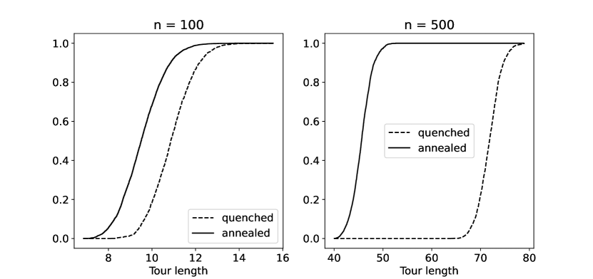
Figure 1: Empirical cumulative distribution functions of $\pi_{\beta}^{q}$ and $\pi_{\beta}^{a}$, for $\beta=10$ at $n=100$ and $n=500$ with $N=50$.

6 Discussion & Open Problems

Our results highlight a connection between the physics of disordered systems, and the probabilistic analysis of simulated annealing. To be precise, in order to analyze the behavior of simulated annealing on random instances, it is natural to define a Gibbs measure which depends on random parameters. This is the exact same situation which occurs in disordered systems. Hence, we believe that advances in the rigorous understanding of the statistical mechanics of disordered systems will be advantageous to algorithms research.

To be more specific, our results hint that simulated annealing with the logarithmic cooling schedule is not an efficient solution method for TSP, even when compared with exact algorithms. For simulated annealing, our results hold for $t=2^{o(n)}$, while the well-known Bellman-Held-Karp algorithm [6, 17] has time complexity $O^{*}(2^{n})$. Thus, based on our results, we believe that SA with logarithmic cooling cannot improve on this complexity, even to a constant approximation ratio, although we lack a formal proof. The logarithmic cooling schedule was previously show to be necessary and sufficient for SA to asymptotically reach the global optimum [16]. This paper is a first step towards a proof that this nice mathematical property should be sacrificed in practice, a fact already well established in practice [2, chapter 8].

The connection between disordered systems and NP-hard problems is not novel, and has been analyzed both from a physical (e.g. [5, 14, 19]) and mathematical [29, 30] perspective. However, much of the research in physics has focused on the limits as $\beta\to\infty$ and $n\to\infty$, referred to in that field as the zero-temperature and thermodynamic limits. Research in mathematics has focused mostly on spin glass systems, $k$-SAT, the random assignment problem, and perceptrons. From that perspective, the main novelty of our results is as a rigorous statement on random TSP instances in the framework of disordered systems, for finite $n$ and at finite temperature, which is of more practical interest to the algorithms community than the aforementioned limiting cases.

To conclude, we list some possible directions for future research on the present topic.

Lower tail bound out of equilibrium.

We have already highlighted one open problem (Section 2.3), which would strengthen our results. Even so, this conjecture is only a statement on the equilibrium behavior of simulated annealing. If it can be shown to hold, an obvious extension would be to the out-of-equilibrium situation, which is more directly applicable to simulated annealing. This seems to be a challenging problem, as it involves the time-dependent distribution of an inhomogeneous Markov chain. Any rigorous results in this direction may also yield insight into nonequilibrium statistical mechanics.

Probabilistic models.

Another clear open problem would be to analyze simulated annealing for different probabilistic TSP models, especially models with dependence between the edge weights. Physicists have previously considered the Euclidean TSP, but rigorous results do not appear to be known. The addition of dependence between edge weights would make our proof of Lemma 3.4 invalid, so this extension would require more advanced proof techniques than the straightforward analysis we have employed.

Relaxed mixing requirements.

In Section 4 we have made some effort to prove statements on simulated annealing outside of equilibrium. The results we have found are however quite restrictive, requiring the Markov chain to be close to equilibrium at all times, and moreover setting strong limits on the cooling schedule. Proving an equivalent to Lemma 4.2 without the assumption that $a\geq n$ is another challenge we have not addressed.

Upper bound on the average case runtime.

While we have in this work set out towards an upper bound on the average case runtime, the reverse problem is also of interest. Since the known worst case results are no improvement over simply picking a tour uniformly at random [1, 16, 26], we expect that it should be possible to show a better upper bound in the average case.

Application to different problems.

Finally, some of our results are quite agnostic with respect to the problem one analyzes. Replacing Lemma 3.4 with the partition function of any other problem would yield results applied to that problem. It may thus be interesting to perform this substitution for different problems, and identify problems for which the negative results suggested by Sections 2.3 and 2.3 are not applicable. These are then problems for which the runtime lower bound we set out to prove may not hold. Thus it may be possible to apply simulated annealing with the logarithmic cooling schedule efficiently to these problems.

Appendix A Proofs Omitted in Section 3

See 3.1

Proof.

We start by noting that $Z(\beta\>\lvert\>W)$ is related to the moment generating function $M_{J}(s\>\lvert\>\cdot)$ of the random variable $J$. To wit,

$$M_{J}(s\>\lvert\>W):=\mathbb{E}_{\pi_{\beta}}\left(e^{sJ}\right)=\sum_{x\in S}e^{sJ(x\>\lvert\>W)}\pi_{\beta}(x\>\lvert\>W)=\frac{\sum_{x\in S}e^{(s-\beta)J(x\>\lvert\>W)}}{\sum_{y\in S}e^{-\beta J(y\>\lvert\>W)}}=\frac{Z(\beta-s\>\lvert\>W)}{Z(\beta\>\lvert\>W)}.$$

Since the cumulant generating function $K_{J}(s\>\lvert\>W)$ is defined as $K_{J}(s\>\lvert\>W):=\ln M_{J}(s\>\lvert\>W)$, we have

$$K_{J}(s\>\lvert\>W)=\ln Z(\beta-s\>\lvert\>W)-\ln Z(\beta\>\lvert\>W).$$

Then we have

$$\kappa_{p}(\beta\>\lvert\>W)=\left.\frac{\partial^{p}}{\partial s^{p}}K_{J}(s\>\lvert\>W)\right|_{s=0}=(-1)^{p}\frac{\partial^{p}}{\partial\beta^{p}}\ln Z(\beta\>\lvert\>W).$$

∎

See 3.3

Proof.

For the first inequality, suppose that is false, and integrate the resulting inequality to obtain

$$\mathbb{E}(\ln Z(\beta\>\lvert\>W))-\mathbb{E}(\ln Z(0\>\lvert\>W))>\ln\mathbb{E}(Z(\beta\>\lvert\>W))-\ln\mathbb{E}(Z(0\>\lvert\>W)).$$

Note that $Z(0\>\lvert\>W)=|S|$, independent of the realization of $W$. Hence, the corresponding terms on both sides cancel, and we are left with a contradiction to Jensen’s inequality.

Now for the second inequality, we proceed similarly, integrating its negation to find

$$\frac{\mathrm{d}}{\mathrm{d}\beta}\mathbb{E}(\ln Z(\beta\>\lvert\>W)) -\left.\frac{\mathrm{d}}{\mathrm{d}\beta}\mathbb{E}(\ln Z(\beta\>\lvert\>W))\right|_{\beta=0}$$

$$>\frac{\mathrm{d}}{\mathrm{d}\beta}\ln\mathbb{E}(Z(\beta\>\lvert\>W))-\left.\frac{\mathrm{d}}{\mathrm{d}\beta}\ln\mathbb{E}(Z(\beta\>\lvert\>W))\right|_{\beta=0}.$$

We show that the second terms on both sides are again equal. Indeed:

$$-\frac{\mathrm{d}}{\mathrm{d}\beta}\mathbb{E}(\ln(Z(\beta\>\lvert\>W)))=\mathbb{E}\left(\sum_{x\in S}\frac{J(x\>\lvert\>W)e^{-\beta J(x\>\lvert\>W)}}{Z(\beta\>\lvert\>W)}\right),$$

and so

$$-\left.\frac{\mathrm{d}}{\mathrm{d}\beta}\mathbb{E}(\ln(Z(\beta\>\lvert\>W)))\right|_{\beta=0}=\mathbb{E}\left(\frac{1}{|S|}\sum_{x\in S}J(x\>\lvert\>W)\right)=\frac{1}{|S|}\sum_{x\in S}\mathbb{E}(J(x\>\lvert\>W)).$$

Meanwhile,

$$-\frac{\mathrm{d}}{\mathrm{d}\beta}\ln\mathbb{E}(Z(\beta\>\lvert\>W))=\frac{1}{\mathbb{E}(Z(\beta\>\lvert\>W))}\mathbb{E}\left(\sum_{x\in S}J(x\>\lvert\>W)e^{-\beta J(x\>\lvert\>W)}\right).$$

Evaluating this at $\beta=0$ yields the same expression once more. Therefore, the corresponding terms once more cancel, leaving us with a contradiction to the first part of the lemma. ∎

See 3.4

Proof.

By definition, we have $Z(\beta\>\lvert\>W)=\sum_{x\in S}e^{-\beta J(x\>\lvert\>W)}$. Recall that $J(x\>\lvert\>W)$ is a sum of edge weights, namely

$$J(x\>\lvert\>W)=\sum_{e\in E(x)}W(e),$$

where $E(x)$ denotes the set of edges present in tour $x$. Hence, the exponential in each term of the partition function can be factored into a product of exponential factors:

$$e^{-\beta J(x\>\lvert\>W)}=\prod_{e\in E(x)}e^{-\beta W(e)}.$$

Using linearity of expectation, we then obtain

$$\mathbb{E}(Z(\beta\>\lvert\>W))=\sum_{x\in S}\prod_{e\in E(x)}\mathbb{E}\left(e^{-\beta W(e)}\right),$$

which holds since the edge weights are independent random variables.

These expectations are easily evaluated:

$$\mathbb{E}\left(e^{-\beta W(e)}\right)=\int_{0}^{1}e^{-\beta y}\mathrm{d}y=\frac{1-e^{-\beta}}{\beta},$$

since $W(e)\sim U[0,1]$. Thus,

$$\mathbb{E}(Z(\beta\>\lvert\>W))=\sum_{x\in S}\left(\frac{1-e^{-\beta}}{\beta}\right)^{n}.$$

The fact that $|S|=\frac{1}{2}(n-1)!$ completes the proof. ∎

Appendix B Proofs Omitted in Section 4

For the following few proofs, recall the definitions stated at the start of Section 4. The mixing time of a Markov chain is related to the spectral properties of its transition matrix. To be precise, for a transition matrix $P$ with stationary distribution $\pi$, let

$$\lambda_{\star}=\max\{|\lambda|:\lambda\in\Lambda(P),\,\lambda\neq 1\}$$

be the largest (in absolute value) eigenvalue of $P$ not associated with $\pi$. Likewise, let

$$\lambda_{1}=\max\{\lambda:\lambda\in\Lambda(P),\,\lambda\neq 1\}.$$

Then the relaxation time of the chain is defined as

$$\tau_{\mathrm{rel}}:=\frac{1}{1-\lambda_{\star}}.$$

The following holds:

Lemma B.1 (Levin & Peres [3, Thm 12.4]).

Let $P$ be the transition matrix of a reversible, irreducible Markov chain with state space $S$, and let $\pi_{\min}:=\min_{x\in S}\pi(x)$. Then

$$\tau(\epsilon)\leq\tau_{\mathrm{rel}}\ln\left(\frac{1}{\epsilon\pi_{\min}}\right).$$

We define the spectral gap of $P$ as $\gamma=1-\lambda_{1}$, and distinguish it from the the absolute spectral gap, $\gamma_{\star}=1-\lambda_{\star}$. This allows us to use a result from Sinclair & Jerrum:

Lemma B.2 (Sinclair & Jerrum [27, Prop. 3.2]).

Let P be the transition matrix of an ergodic time-reversible Markov chain, and $1=\lambda_{0}>\lambda_{1}>\ldots>\lambda_{N-1}>-1$ its eigenvalues. Then the modified chain with transition matrix $P^{\prime}=\frac{1}{2}(I_{N}+P)$ is also ergodic and time-reversible with the same stationary distribution, and its eigenvalues $\{\lambda_{i}^{\prime}\}$, similarly ordered, satisfy $\lambda^{\prime}_{N-1}>0$ and $\lambda^{\prime}_{\max{}}=\lambda_{1}^{\prime}=\frac{1}{2}(1+\lambda_{1})$.

The modified chain in this proposition is easily constructed from the original chain. At each iteration, one first flips a coin. On heads, the chain stays in the current state. On tails, the usual Metropolis trial is conducted. Such a chain is called a lazy Markov chain [3].

Given any realization of this lazy chain, we can obtain a realization of the original Markov chain by removing certain elements from the generated sequence of states. Since the chains share their stationary distribution, this implies that the mixing time of the original chain is at most that of the lazy chain. In the following few lemmas, we consider only the lazy chain. The reason for this switch is that for the lazy chain, we have $\gamma_{\star}=\gamma$, which is easier to bound.

Finally, we quote two more results: one relating the spectral gap of a transition matrix to the structure of the underlying state graph, and one relating the spectral gap to the bottleneck ratio of the chain. The bottleneck ratio of a Markov chain with transition matrix $P$ and stationary distribution $\pi$ is defined as

$$\Phi_{\star}:=\min_{\begin{subarray}{c}S\subset V\\ \pi(S)\leq 1/2\end{subarray}}\frac{\sum_{x\in S}\sum_{y\in V\setminus S}\pi(x)P(x,y)}{\pi(S)},$$

where $\pi(S)=\sum_{x\in S}\pi(x)$.

Lemma B.3 (Levin & Peres [3, Thm. 13.26]).

Let $G$ be a transitive graph with vertex degree $d$ and diameter $D$. For the simple random walk on $G$,

$$\frac{1}{\gamma}\leq 2dD^{2}.$$

Lemma B.4 (Sinclair & Jerrum (1989), Lawler & Sokal (1988) [3, Thm. 13.10]).

Let $\lambda_{1}$ be the second largest eigenvalue of a reversible transition matrix $P$, and let $\gamma=1-\lambda_{1}$. Then

$$\frac{\Phi_{\star}^{2}}{2}\leq\gamma\leq 2\Phi_{\star}.$$

See 4.1

Proof.

Let $P_{t}$ be the transition matrix of the Markov chain of lazy simulated annealing at inverse temperature $\beta_{t}=\ln t/a$. Let $\Phi(t)$ denote the bottleneck ratio of the Markov chain at inverse temperature $\beta_{t}$, and let $\Phi_{0}=\lim_{t\to 0}\Phi(t)$.

Following a proof by Nolte and Schrader [25, Theorem 1], we have

$$\Phi(t)\geq\Phi_{0}t^{-J_{\max}/a}\geq\frac{\Phi_{0}}{t}.$$

From the definition of $\Phi_{\star}$, one easily sees that the bottleneck ratio of a lazy Markov chain is identical to that of the original chain, multiplied by a factor of $1/2$. After all, the off-diagonal elements of the lazy transition matrix are simply those of the original matrix multiplied by $1/2$, and only these elements appear in the definition of $\Phi_{\star}$. Hence, letting $\Phi$ denote the bottleneck ratio of the simple random walk, we find $\Phi(t)\geq\Phi_{0}/t=\Phi/(2t)$.

Lemma B.4 tells us that $\Phi\geq\gamma/2$, where $\gamma$ denotes the spectral gap of $P_{0}$. Now by Lemma B.3, we have

$$\gamma\geq\frac{1}{2dD^{2}}.$$

Putting all this together, we arrive at

$$\Phi(t)\geq\frac{\Phi}{2t}\geq\frac{\gamma}{4t}\geq\frac{1}{8dD^{2}t}.$$

Then by Lemma B.4,

$$\lambda_{\star}\leq 1-\frac{\Phi(t)^{2}}{2}\leq 1-\frac{1}{128d^{2}D^{4}t^{2}}.$$

Now by Lemma B.1,

$$\tau(\epsilon)\leq\frac{1}{1-\lambda}\ln\left(\frac{1}{\epsilon\min_{x\in S}\pi_{t}(x)}\right)\leq 128d^{2}D^{4}t^{2}\ln\left(\frac{1}{\epsilon\min_{x\in S}\pi_{t}(x)}\right).$$

The stationary distribution has a straightforward lower bound:

$$\pi_{t}(x)=\frac{1}{Z(\beta_{t}\>\lvert\>w)}e^{-\beta_{t}J(x)}\geq\frac{1}{Z(\beta_{t}\>\lvert\>w)}e^{-\beta_{t}J_{\max}}\geq\frac{1}{|S|}e^{-\beta_{t}J_{\max}},$$

which follows from the fact that $Z(\beta_{t}\>\lvert\>w)\leq|S|$. Hence,

$$\tau(\epsilon)\leq 128d^{2}D^{4}t^{2}\ln\left(\frac{|S|e^{\beta_{t}J_{\max}}}{\epsilon}\right)\leq 128d^{2}D^{4}t^{2}\ln\left(\frac{|S|t}{\epsilon}\right).$$

Since the mixing time of a lazy Markov chain is an upper bound to the mixing time of the original chain, we are done. ∎

See 4.2

Proof.

For notational convenience, denote $\mathbb{E}_{\nu}(\cdot\>\lvert\>W)$ by $\langle\cdot\rangle_{\nu}$ for a conditional probability measure $\nu(\cdot\>\lvert\>W)$ defined on $S$. Similarly, we will suppress the dependence of $\nu_{r}$, $\pi_{t}$ and $J$ on $W$ as it plays no role in this proof. We begin by bounding the difference in expectation of $J$ taken over $\pi_{t+1}$ and $\nu_{r}$,

$$\left|\langle J\rangle_{\nu_{r}}-\langle J\rangle_{\pi_{t+1}}\right| =\left|\sum_{x\in S}J(x)(\nu_{r}(x)-\pi_{t+1}(x))\right|$$

$$=\left|\sum_{x\in S}J(x)\sqrt{\pi_{t+1}(x)}\frac{\nu_{r}(x)-\pi_{t+1}(x)}{\sqrt{\pi_{t+1}(x)}}\right|,$$

which is permissible since $\pi_{t+1}(x)>0$ for all $x$ when $t<\infty$. Let $\Pi_{t}=\operatorname{diag}(\pi_{t})$, and consider $J\in\mathbb{R}^{|S|}$ as a vector on $S$. Then the above can be cast as

$$\left|\langle J\rangle_{\nu_{r}}-\langle J\rangle_{\pi_{t+1}}\right|=\left|\left\langle\Pi_{t+1}^{1/2}J,\Pi_{t+1}^{-1/2}(\nu_{r}-\pi_{t+1})\right\rangle\right|\leq\|\Pi_{t+1}^{1/2}J\|_{2}\left\|\Pi_{t+1}^{-1/2}(\nu_{r}-\pi_{t+1})\right\|_{2},$$

where $\langle\cdot,\cdot\rangle$ denotes the standard Euclidean inner product. Now, we define the weighted norm

$$\|u\|_{t}:=\sqrt{\sum_{x\in S}\frac{u(x)^{2}}{\pi_{t}(x)}}=\|\Pi_{t}^{-1/2}u\|_{2}.$$

Furthermore, notice that $\|\Pi_{t+1}^{1/2}J\|_{2}=\sqrt{\langle J^{2}\rangle_{\pi_{t+1}}}$. Hence,

$$\left|\langle J\rangle_{\nu_{r}}-\langle J\rangle_{\pi_{t+1}}\right|\leq\sqrt{\langle J^{2}\rangle_{\pi_{t+1}}}\|\nu_{r}-\pi_{t+1}\|_{t+1}\leq n\|\nu_{r}-\pi_{t+1}\|_{t+1},$$

since $J(x)\leq n$ for all $x\in S$. It then remains to show a suitable bound for $\|\nu_{r}-\pi_{t+1}\|_{t+1}$. To that end, the following fact is useful.

Claim.

For $A\in\mathbb{R}^{|S|\times|S|}$, let $\|A\|_{t}$ denote the matrix norm induced by $\|\cdot\|_{t}$. We have $\|P_{t}\|_{t}=1$.

Proof.

By the definition of $\|\cdot\|_{t}$, it follows that $\|A\|_{t}=\|\Pi_{t}^{1/2}A\Pi_{t}^{-1/2}\|_{2}$. Define $Q_{t}=\Pi_{t}^{1/2}P_{t}\Pi_{t}^{-1/2}$. One can show that under detailed balance for $P_{t}$, the matrix $Q_{t}$ is symmetric. As a result, $\|Q_{t}\|_{2}=\max_{\lambda\in\Lambda(Q_{t})}|\lambda|$, where $\Lambda(A)$ denotes the spectrum of the operator $A$. Since $Q_{t}$ and $P_{t}$ are similar, $\Lambda(Q_{t})=\Lambda(P_{t})$, and since $P_{t}$ is stochastic, its largest eigenvalue in absolute value is $1$. Putting all this together leads us to conclude $\|P_{t}\|_{t}=1$. ∎

Armed with this fact and the sub-multiplicativity of the matrix norm, we find

$$\|\nu_{r}-\pi_{t+1}\|_{t+1}=\|(\nu_{0}-\pi_{t+1})P_{t+1}^{r}\|_{t+1}\leq\|\nu_{0}-\pi_{t+1}\|_{t+1}\|P_{t+1}\|_{t+1}^{r}=\|\nu_{0}-\pi_{t+1}\|_{t+1}.$$

Applying the triangle inequality,

$$\|\nu_{0}-\pi_{t+1}\|_{t+1}\leq\|\pi_{t+1}-\pi_{t}\|_{t+1}+\|\nu_{0}-\pi_{t}\|_{t+1}.$$

For the first term, by a result of Nolte & Shrader [25], we have

$$\|\pi_{t+1}-\pi_{t}\|_{t+1}\leq\sqrt{\frac{1}{t}}.$$

For the second term,

$$\|\nu_{0}-\pi_{t}\|_{t+1}\leq\left\|\Pi_{t+1}^{-1/2}\right\|_{2}\|\nu_{0}-\pi_{t}\|_{2}\leq\frac{\|\nu_{0}-\pi_{t}\|_{2}}{\sqrt{\min_{x\in S}\pi_{t+1}(x)}}.$$

Using the same lower bound on $\pi_{t+1}$ as in the proof of Lemma 4.1:

$$\min_{x\in S}\pi_{t+1}(x)\geq\frac{1}{|S|(t+1)},$$

as $Z(\beta\>\lvert\>W)\leq|S|$ and $a\geq n\geq J(x)$ for all $x\in S$. Hence,

$$\|\nu_{0}-\pi_{t}\|_{t+1} \leq\sqrt{|S|(t+1)}\|\nu_{0}-\pi_{t}\|_{2}\leq\sqrt{|S|(t+1)}\|\nu_{0}-\pi_{t}\|_{1}$$

$$=2\sqrt{|S|(t+1)}\|\nu_{0}-\pi_{t}\|_{\mathrm{TV}}.$$

Since by assumption $\|\nu_{0}-\pi_{t}\|_{\mathrm{TV}}\leq\frac{1}{|S|}$,

$$\|\nu_{0}-\pi_{t}\|_{t+1}\leq 2\sqrt{\frac{t+1}{|S|}}.$$

Now recall that $t=2^{o(n)}$. Therefore, since $|S|=(n-1)!/2$, we have $(t+1)/|S|=2^{o(n)}/|S|\leq 2^{-O(n)}=O(1/t)$. We then conclude that

$$\|\nu_{0}-\pi_{t}\|_{t+1}=O\left(\sqrt{\frac{1}{t}}\right).$$

Putting these two bounds together, we have

$$\|\nu_{0}-\pi_{t+1}\|_{t+1}=O\left(\sqrt{\frac{1}{t}}\right),$$

which proves the first part of the lemma. The second part of the lemma follows directly, since we have

$$\mathbb{E}_{\nu_{r}}(J\>\lvert\>W)\geq\mathbb{E}_{\pi_{t+1}}(J\>\lvert\>W)-O\left(\frac{n}{\sqrt{t}}\right).$$

Using the lower bound from Section 2.3, the result follows. ∎

Appendix C Proofs Omitted in Section 5

See 5.1

Proof.

We have

$$\mathbb{P}(J_{a}\leq j)=\frac{\int_{0}^{j}\rho(j^{\prime})e^{-\beta j^{\prime}}\mathrm{d}j^{\prime}}{Z_{a}(\beta)/|S|},$$

where $Z_{a}(\beta)=\mathbb{E}_{\mu}(Z(\beta\>\lvert\>W))$, and

$$\mathbb{P}(J_{q}\leq j)=\int_{[0,1]^{m}}\mu(w)\frac{\int_{0}^{j}\rho(j^{\prime}\>\lvert\>W=w)e^{-\beta j^{\prime}}\mathrm{d}j^{\prime}}{\int_{0}^{n}\rho(j^{\prime}\>\lvert\>W=w)e^{-\beta j^{\prime}}\mathrm{d}j^{\prime}}\mathrm{d}w.$$

By Lemma 3.4,

$$Z_{a}(\beta)=|S|\left(\frac{1-e^{-\beta}}{\beta}\right)^{n}=\left(\frac{1-e^{-\beta}}{\beta}\right)^{n},$$

since for $n=3$, we have $|S|=1$. Moreover, since there is only one tour, $\mathbb{P}(J_{q}\leq j)$ reduces to $F_{\rho}(j)$, the CDF of $\rho$. For $J_{a}$, we find

$$\mathbb{P}(J_{a}\leq j) =\left(\frac{\beta}{1-e^{-\beta}}\right)^{n}\int_{0}^{j}\rho(j^{\prime})e^{-\beta j^{\prime}}\mathrm{d}j^{\prime}$$

$$=\left(\frac{\beta}{1-e^{-\beta}}\right)^{n}\mathbb{E}_{\rho}(e^{-\beta J}\>\lvert\>J\leq j)F_{\rho}(j)$$

$$\geq\left(\frac{\beta}{1-e^{-\beta}}\right)^{n}\mathbb{E}_{\rho}(e^{-\beta J})F_{\rho}(j)$$

$$=F_{\rho}(j)=\mathbb{P}(J_{q}\leq j).$$

Hence, $\mathbb{P}(J_{q}\geq j)\geq\mathbb{P}(J_{a}\geq j)$, and therefore $J_{q}\succeq J_{a}$ for $n=3$. ∎

References

- [1] Emile Aarts and Jan Korst “Simulated annealing and Boltzmann machines: a stochastic approach to combinatorial optimization and neural computing” USA: John Wiley & Sons, Inc., 1989
- [2] “Local Search in Combinatorial Optimization” Princeton University Press, 2003 DOI: 10.2307/j.ctv346t9c
- [3] David Aldous “Markov Chains and Mixing Times (Second Edition) by David A. Levin and Yuval Peres” In The Mathematical Intelligencer 41.1, 2019, pp. 90–91 DOI: 10.1007/s00283-018-9839-x
- [4] David Arthur, Bodo Manthey and Heiko Röglin “Smoothed Analysis of the k-Means Method” In Journal of the ACM 58.5, 2011, pp. 19:1–19:31 DOI: 10.1145/2027216.2027217
- [5] G. Baskaran, Yaotian Fu and P.. Anderson “On the statistical mechanics of the traveling salesman problem” In Journal of Statistical Physics 45.1, 1986, pp. 1–25 DOI: 10.1007/BF01033073
- [6] R. Bellman “Dynamic Programming Treatment of the Travelling Salesman Problem” In JACM, 1962 DOI: 10.1145/321105.321111
- [7] Barun Chandra, Howard Karloff and Craig Tovey “New Results on the Old k-opt Algorithm for the Traveling Salesman Problem” Publisher: Society for Industrial and Applied Mathematics In SIAM Journal on Computing 28.6, 1999, pp. 1998–2029 DOI: 10.1137/S0097539793251244
- [8] Vincent Cohen-Addad and Claire Mathieu “Effectiveness of Local Search for Geometric Optimization” ISSN: 1868-8969 In 31st International Symposium on Computational Geometry (SoCG 2015) 34, Leibniz International Proceedings in Informatics (LIPIcs) Dagstuhl, Germany: Schloss Dagstuhl–Leibniz-Zentrum fuer Informatik, 2015, pp. 329–343 DOI: 10.4230/LIPIcs.SOCG.2015.329
- [9] E.L. Lawler et al. “Chapter 6: Probabilistic analysis of heuristics” In The Traveling Salesman Problem; A Guided Tour of Combinatorial Optimization Wiley, Chichester, 1985 URL: https://ir.cwi.nl/pub/18054
- [10] Christian Engels and Bodo Manthey “Average-case approximation ratio of the 2-opt algorithm for the TSP” In Operations Research Letters 37.2, 2009, pp. 83–84 DOI: 10.1016/j.orl.2008.12.002
- [11] Matthias Englert, Heiko Röglin and Berthold Vöcking “Worst Case and Probabilistic Analysis of the 2-Opt Algorithm for the TSP” In Algorithmica 68.1, 2014, pp. 190–264 DOI: 10.1007/s00453-013-9801-4
- [12] U. Faigle and W. Kern “Note on the Convergence of Simulated Annealing Algorithms” Publisher: Society for Industrial and Applied Mathematics In SIAM Journal on Control and Optimization 29.1, 1991, pp. 153–159 DOI: 10.1137/0329008
- [13] Alan Frieze “On Random Symmetric Travelling Salesman Problems” Publisher: INFORMS In Mathematics of Operations Research 29.4, 2004, pp. 878–890 URL: https://www.jstor.org/stable/30035650
- [14] Y. Fu and P.. Anderson “Application of statistical mechanics to NP-complete problems in combinatorial optimisation” Publisher: IOP Publishing In Journal of Physics A: Mathematical and General 19.9, 1986, pp. 1605–1620 DOI: 10.1088/0305-4470/19/9/033
- [15] Stuart Geman and Donald Geman “Stochastic Relaxation, Gibbs Distributions, and the Bayesian Restoration of Images” Conference Name: IEEE Transactions on Pattern Analysis and Machine Intelligence In IEEE Transactions on Pattern Analysis and Machine Intelligence PAMI-6.6, 1984, pp. 721–741 DOI: 10.1109/TPAMI.1984.4767596
- [16] Bruce Hajek “Cooling Schedules for Optimal Annealing” Publisher: INFORMS In Mathematics of Operations Research 13.2, 1988, pp. 311–329 URL: https://www.jstor.org/stable/3689827
- [17] Michael Held and Richard M. Karp “A Dynamic Programming Approach to Sequencing Problems” Publisher: Society for Industrial and Applied Mathematics In Journal of the Society for Industrial and Applied Mathematics 10.1, 1962, pp. 196–210 URL: https://www.jstor.org/stable/2098806
- [18] R. Karp “A Patching Algorithm for the Nonsymmetric Traveling-Salesman Problem” In SIAM J. Comput., 1979 DOI: 10.1137/0208045
- [19] Scott Kirkpatrick and Bart Selman “Critical Behavior in the Satisfiability of Random Boolean Expressions” Publisher: American Association for the Advancement of Science In Science 264.5163, 1994, pp. 1297–1301 DOI: 10.1126/science.264.5163.1297
- [20] Bernhard Korte and Jens Vygen “Combinatorial Optimization: Theory and Algorithms”, Algorithms and Combinatorics Berlin Heidelberg: Springer-Verlag, 2000 DOI: 10.1007/978-3-662-21708-5
- [21] “The physics of disordered systems” New Delhi, India: Hindustan Book Agency, 2012
- [22] Nicholas Metropolis et al. “Equation of State Calculations by Fast Computing Machines” Publisher: American Institute of Physics In The Journal of Chemical Physics 21.6, 1953, pp. 1087–1092 DOI: 10.1063/1.1699114
- [23] Wil Michiels, Jan Korst and Emile Aarts “Properties of Neighborhood Functions” In Theoretical Aspects of Local Search, Monographs in Theoretical Computer Science, An EATCS Series Berlin, Heidelberg: Springer, 2007, pp. 53–61 DOI: 10.1007/978-3-540-35854-1˙4
- [24] Alexander M. Mood et al. “Introduction to the Theory of Statistics” McGraw-Hill, 1973
- [25] Andreas Nolte and Rainer Schrader “A Note on the Finite Time Behavior of Simulated Annealing” Publisher: INFORMS In Mathematics of Operations Research 25.3, 2000, pp. 476–484 URL: https://www.jstor.org/stable/3690480
- [26] Sanguthevar Rajasekaran “On the Convergence Time of Simulated Annealing” In Technical Reports (CIS), 1990 URL: https://repository.upenn.edu/cis_reports/356
- [27] Alistair Sinclair and Mark Jerrum “Approximate counting, uniform generation and rapidly mixing Markov chains” In Information and Computation 82.1, 1989, pp. 93–133 DOI: 10.1016/0890-5401(89)90067-9
- [28] Alan Stuart and Keith Ord “Kendall’s Advanced Theory of Statistics, Volume 1, Distribution Theory” Wiley, 2010 URL: https://www.wiley.com/en-us/Kendall%27s+Advanced+Theory+of+Statistics%2C+Volume+1%2C+Distribution+Theory%2C+6th+Edition-p-9780470665305
- [29] Michel Talagrand “The high temperature case for the random K-sat problem” In Probability Theory and Related Fields 119.2, 2001, pp. 187–212 DOI: 10.1007/PL00008758
- [30] Michel Talagrand and chel Talagrand “Spin Glasses: A Challenge for Mathematicians: Cavity and Mean Field Models” Springer Science & Business Media, 2003
- [31] Andrea Vattani “k-means Requires Exponentially Many Iterations Even in the Plane” In Discrete & Computational Geometry 45.4, 2011, pp. 596–616 DOI: 10.1007/s00454-011-9340-1