Identifying atmospheric fronts based on diabatic processes using the dynamic state index (DSI)

Laura Mack^1,*, Annette Rudolph¹, Peter Névir¹

1: Institute of Meteorology, Freie Universität Berlin, Germany
*: Correspondence: laura.mack@fu-berlin.de

Abstract

Atmospheric fronts are associated with precipitation and strong diabatic processes. Therefore, detecting fronts objectively from reanalyses is a prerequisite for the long-term study of their weather impacts. For this purpose, several algorithms exist, e.g., based on the thermic front parameter (TFP) or the F diagnostic. It is shown that both methods have problems to identify weak warm fronts since they are characterized by low baroclinicity. To avoid this inaccuracy, a new algorithm is developed that considers fronts as deviation from an adiabatic and steady state. These deviations can be accurately measured using the dynamic state index (DSI). The DSI shows a coherent dipole structure along fronts and is strongly correlated with precipitation sums. It is shown that the North Atlantic storm tracks can be clearly identified by the DSI method. Compared to other front identification methods, fronts identified with the DSI method have particularly high specific humidity. Using a simple estimate for front speed, it is shown that fronts identified using DSI method move faster then fronts identified with TFP method, demonstrating the potential of the DSI to indicate movement speed and direction in atmospheric flows.

Keywords: Front Identification, Front Detection, Front Climatology, Front Speed, Dynamic State Index

1 Introduction

Fronts are essential features of extratropical cyclones (Bjerknes and Solberg, , 1922) and are responsible for extreme precipitation and wind gusts (e.g., Catto et al., (2012); Catto and Pfahl, (2013); Raveh-Rubin and Catto, (2019)). On weather maps, fronts are drawn based on the temperature difference they cause. However, the extreme weather events associated with fronts show that fronts are additionally associated with complex dynamics, e.g., they represent an area of maximum relative vorticity (Hoskins, , 1982). Therefore, it is particularly interesting to study fronts from the perspective of vorticity dynamics.
In order to study the location, frequency, and intensity of fronts, they must first be identified. Meteorologists use several parameters for front identification, e.g. temperature, dew point or wind direction. Thus different meteorologists identify different fronts, which is why this type of front identification is called ’subjective’ (Uccellini et al., , 1992). Hewson, (1998) pointed out the advantages of automated and reproducible algorithms for front identification, which are referred to as ’objective’ methods. Accordingly, the methods that are used should be simple, intelligible, accurate, tunable and portable. But even for these ’objective’ methods, suitable meteorological variables and threshold values must first be found. Since there is no widely accepted definition of fronts, different quantities can be used for this purpose. Thermal quantities, which are called primary (defining) quantities, are often preferred, since secondary quantities, such as vorticity, cannot unambiguously identify fronts (Thomas and Schultz, , 2019). However, precisely these secondary dynamic variables are often associated with extreme weather events occurring at fronts (e.g., Grazzini et al., (2020); Solari et al., (2022)).
Classical methods use thermal (i.e. primary) quantities, such as the thermic front parameter (TFP) or the horizontal temperature gradient (e.g., Hewson, (1998); Berry et al., (2011); Catto and Pfahl, (2013)). To include dynamic properties of fronts, Parfitt et al., (2017) suggest an empirical function, called F diagnostic, which combines the horizontal temperature gradient with the relative vorticity. The problem with this approach is that these two quantities used are not independent of each other. Both quantities are positively correlated via the frontal transverse circulation (Hoskins, , 1982), so that the product of them increases unintentionally the difference between strong and weak fronts. To avoid this, we are developing a new method that considers only one quantity, but still captures vortex dynamic aspects of fronts and their weather influence. For this we consider fronts as deviations from a dynamical basic state derived directly from the primitive equations. This basic state is characterized by stationarity and adiabasia. The deviations from this basic state can be measured with the dynamic state index (DSI) (Névir, , 2004; Weber and Névir, , 2008). This new method therefore allows fronts to be identified, based on the diabatic processes occurring at them, and is thus linked to extreme precipitation associated with fronts (Claussnitzer et al., , 2008; Claussnitzer, , 2010; Müller et al., , 2018).
This paper addresses the following research questions:

1. What does the DSI structure of fronts look like?

2. How can fronts be identified using the DSI?

3. How does the new DSI method differ statistically from state-of-the-art front detection methods?

In Chap. 2, the existing front identification methods based on TFP and F diagnostic are explained and visualized with a case study. Then, the DSI is introduced and it is shown how the DSI reflects fronts. Based on this, the new front identification method (”DSI method”) is introduced (Chap. 3). Chap. 4 compares the three methods based on their annual cycle and examines which properties the detected fronts have. Chap. 5 summarizes and discusses the results.

2 Front identification

The general procedure for identifying fronts from gridded data is to use one or more meteorological input variables, apply a function to them, and then test for a threshold exceedance. At the end, graphical filters can be applied, e.g. to delete disconnected pixels (see, e.g., Berry et al., (2011); Kern et al., (2019)). To be able to compare the methods and the influence of the input variables directly with each other, no filters are used in this study. In this chapter the two state-of-the-art front identification methods according to Hewson, (1998) and Parfitt et al., (2017) are explained and applied directly to a case study (a rapid cyclogenesis caused by a dry intrusion occurring in February 2014 over the North Atlantic) using the ERA5 reanalysis on pressure levels with a horizontal resolution of 0.25^∘$\times$0.25^∘ (Hersbach et al., , 2020). First, the weather situation is presented and then the front identification methods are explained.

2.1 Case study: Rapid cyclogenesis 14.02.2014

Fig. 1 shows a trough west of Ireland at 14.02.2014 12 UTC with a low pressure system on its southeastern side, which is partly occluded and clearly shows a warm front (over France) and a cold front (west of Portugal). The jet stream flows over the cold front, so that it has cata character in the northern part and ana character in the southern part. Along the fronts the specific humidity is particularly high. Maxima of the vertical velocity can be seen in the area of the occlusion and at the back of the ana cold front. This depression was part of a series of rapid intensifying cyclones over the North Atlantic in February 2014 (see, e.g., Volonté et al., (2018)) and was studied by Bott, (2016) in terms of precipitation.

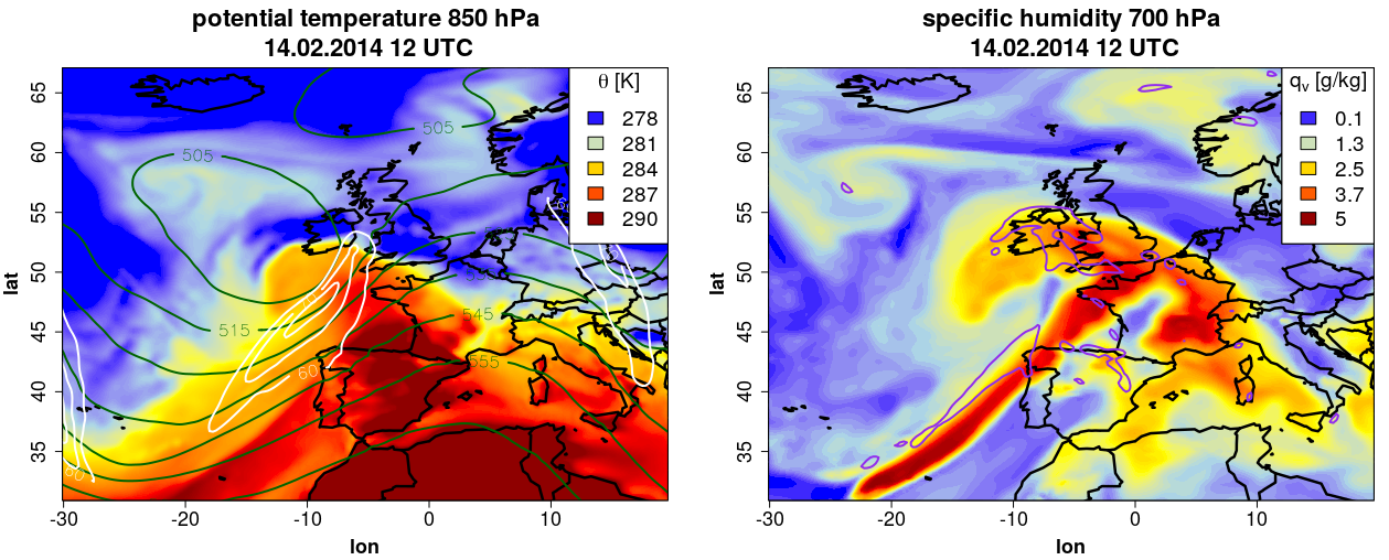
Figure 1: Weather situation 14.02.2014 12 UTC. Left: Potential temperature at 850 hPa with contour lines of geopotential height at 500 hPa (darkgreen, in gpdm) and of the horizontal wind at 300 hPa (white, in m/s). Right: Specific humidity at 700 hPa with contour line of -1 Pa/s updraft (purple).

2.2 Method 1: Thermic front parameter

Hewson, (1998) developed a front identification method based on the thermic front parameter (TFP). The TFP was introduced by Renard and Clarke, (1965) based on a general thermic quantity $\tau$ by

$$TFP({\tau}):=-\nabla_{h}\|\nabla_{h}\tau\|\cdot\dfrac{\nabla_{h}\tau}{\|\nabla_{h}\tau\|}.$$ (1)

Thereby, the gradient of the baroclinicity measured by $\|\nabla_{h}\tau\|$ is projected on the horizontal unit vector (second factor). For $\tau$ often the potential temperature or the equivalent-potential temperature is used. Thomas and Schultz, (2019) showed, that using $\theta_{e}$ (for front detection) leads to artificial fronts in the tropical regions due to high moisture content. To avoid this problem we use $\tau=\theta$. Fig. 2 shows the TFP at 850 hPa exemplary for the considered case study. The TFP has a dipole structure, with negative values at the front side of the warm front and the occluded front, and positive values at the front side of the cold front. The cata cold front is not visible in the TFP, so the cold front is detached from the frontal system, which is a characteristic feature of Shapiro-Keyser lows (Shapiro and Keyser, , 1990).

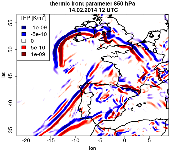
Figure 2: Thermic front parameter (TFP) at 850 hPa, 14.02.2014 12 UTC.

Using the TFP concept Hewson, (1998) developed an algorithm that allows the detection of fronts as front lines as well as frontal zones:

  Algorithm 1: Front identification using TFP according to Hewson, (1998)

  front lines

front locator: $$\frac{\partial(\|\nabla_{h}\|\nabla_{h}\tau\|\|)}{\partial\hat{s}}=0\;\textrm{ with }\;\hat{s}=\frac{\nabla_{h}\|\nabla_{h}\tau\|}{\|\nabla_{h}\|\nabla_{h}\tau\|\|}$$ (2)

$$\nabla TFP(\tau)\cdot\frac{\nabla_{h}\tau}{\|\nabla_{h}\tau\|}=0$$ (3)

masking variable 1: $$TFP({\tau})>K_{1}$$ (4)

masking variable 2: $$S({\tau}):=\|\nabla_{h}\tau\|>K_{2}$$ (5)

$$\vdots\hskip 85.35826pt$$

masking variable n

  frontal zones

$$TFP({\tau})>K_{1}$$ (6)

 

First, the location of the front line is determined. In the frontal zone the gradient of the thermal quantity $\tau$ is the largest, so that the first partial derivative has a maximum there. The second spatial derivative has a minimum at the front of the frontal zone (which is called front line) and the third derivative a root, which must be determined (see, Kern et al., (2019) their Fig. 2 and 3). In order to additionally take into account the curvature of the front, the divergence along the unit vector $\hat{s}$ is considered resulting in Eq. 2, which was simplified by Huber-Pock and Kress, (1981) to Eq. 3. To filter out the front, masking conditions are applied. The first masking condition (Eq. 4) states that the TFP must have a minimum value of $K_{1}$. The value of $K_{1}$ depends on the used thermal quantity, the pressure level and the grid size. Here we follow Kern et al., (2019) and use $K_{1}=0.3\cdot 10^{-10}$ K/m for 850 hPa level, which is similar to Hewson, (1998) and Parfitt et al., (2017) ($K_{1}=0.33\cdot 10^{-10}$ K/m for 900 hPa) but different from Catto and Pfahl, (2013) ($K_{1}=-8\cdot 10^{-12}$ K/m for the wet bulb potential temperature at 850 hPa). Fig. 3 (left part) shows the front locator (thin red lines), the first masking condition (orange shading) and the intersection of both resulting in the (preliminary) front lines (thick red lines). The occlusion front, warm front, ana cold front and also a part of the cata cold front displaced to the ana cold front are detected. To further filter the front lines, Hewson, (1998) uses the strength of the front $S(\tau)$ given by Eq. 5. If the second masking condition is applied (Fig. 3, right part), then only the part of the (preliminary) front lines from the first masking step are kept which also show a minimum strength. Due to the lower baroclinicity, the warm front and a part of the occlusion front are now not captured, even when using a comparatively small threshold of $K_{2}=1.35\cdot 10^{-5}$ K/m (Hewson, , 1998; Parfitt et al., , 2017; Kern et al., , 2019). Since this is not intentional, we use only the first masking step in this study. This also allows filtering for frontal zones directly (Eq. 6). Consequently, warm fronts are located at the end of the warm air advection and cold fronts at the beginning of the cold air advection.

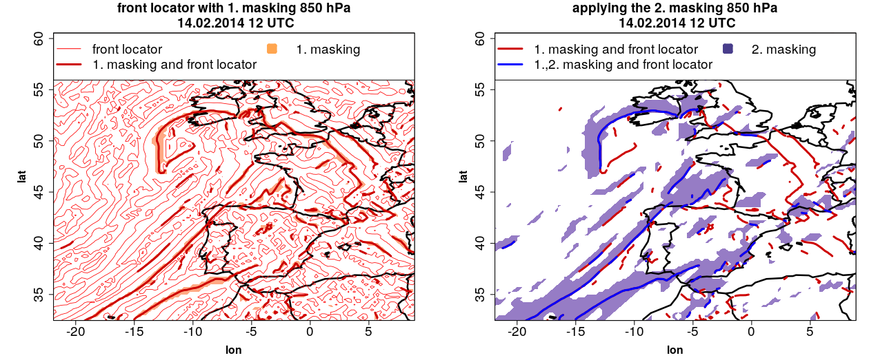
Figure 3: Front identification using the TFP method. Left: Front locator (thin red line), the first masking condition (orange shade) and the intersection of both (thick red line). Right: Results from the first masking step (thick red line), the second masking condition (blue shade) and the intersection of both (thick blue line).

2.3 Method 2: F diagnostic

Parfitt et al., (2017) use the fact that fronts are regions of high temperature gradients and maximal vorticity to develop a new front identification method, which only allows the detection of frontal zones (and not lines):

  Algorithm 2: Front identification using F diagnostic according to Parfitt et al., (2017)  

$$\textrm{defining quantity:}\quad F :=\frac{\zeta}{f}\frac{\|\nabla_{h}T\|}{\|\nabla_{h}T\|_{0}}$$ (7)

$$\textrm{masking:}\quad F \begin{cases}>1,&\textrm{for low-level fronts}\\ >2,&\textrm{for upper-level fronts (from 600 hPa)}\end{cases}$$ (8)

 

F is an empirically determined and dimensionless function containing the relative vorticity $\zeta$, the Coriolis parameter $f$, the temperature $T$ and an empirical determined constant $\|\nabla T\|_{0}=0.45$ K/(100 km). The threshold values used for masking (Eq. 8) were also determined empirically based on ERA-Interim.
We point out that F contains the Rossby number

$$Ro:=\frac{\zeta}{f}\begin{cases}\ll 1\;&\rightarrow\textrm{synoptic scale}\\ \approx 1\;&\rightarrow\textrm{mesoscale}\\ \gg 1\;&\rightarrow\textrm{convective scale},\end{cases}$$ (9)

which describes the ratio of inertia to Coriolis force and can be taken as a measure for the spatial scale. When using the F diagnostic, fronts are perceived on the basis of their spatial scale weighted with the horizontal temperature gradient. The F diagnostic (Fig. 4, left part) shows high values in the low center and along the occlusion front due to high relative vorticity caused by the dry intrusion. Along the ana cold front and partly in the warm front region F also shows positive values. If now the masking condition $F>1$ is applied, the frontal zones shown in the right part of Fig. 4 result. Thereby, the low center is erroneously detected as a front and the warm and cold fronts are detected only to a small part detached from the low center. Since baroclinicity and relative vorticity are not independent of each other but are positively correlated (Hoskins, , 1982), only particularly strong fronts are detected with the F diagnostic.

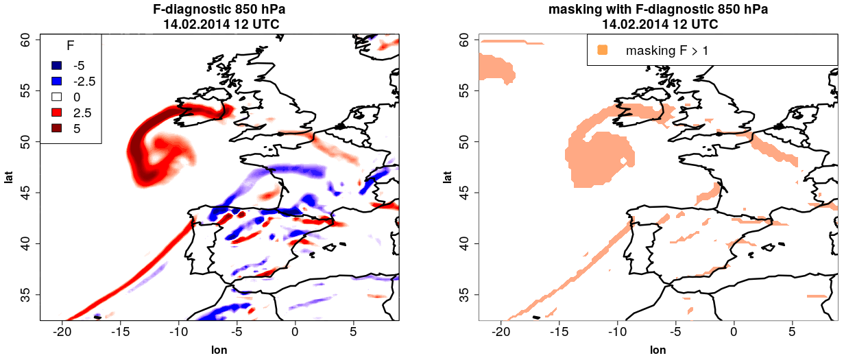
Figure 4: Front identification using the F diagnostic. Left: F diagnostic at 850 hPa. Right: Masking condition $F>1$.

3 The dynamic state index (DSI) and its relation to atmospheric fronts

In this chapter the concept of the dynamic state index (DSI) is presented. Using the case study from before the DSI structure of fronts is investigated. Based on these results we develop a new algorithm for front identification.

3.1 The concept of the dynamic state index (DSI)

In order to investigate flows systematically, they are often divided into a basic state and a deviation from it. This basic state can, for example, be determined statistically with the mean value. The deviation is then given in first order by the standard deviation. This statistical approach has the disadvantage that the mean value does not necessarily represent a solution of the basic equation system and is therefore not balanced. Therefore, a dynamic basic state is needed, which is itself a solution to the primitive equations. We use an adiabatic and stationary basic state whose deviations are then given by the DSI (Névir, , 2004; Weber and Névir, , 2008). This has the advantage that the basic state is balanced. However, the deviations from the basic state, i.e., the DSI, must first be derived.
The starting point for deriving the DSI is the Navier-Stokes equation on a rotating Earth with friction under dry conditions

$$\frac{d\boldsymbol{v}}{dt}+2\boldsymbol{\omega}\times\boldsymbol{v}=-\frac{1}{\rho}\nabla p-\nabla\Phi+\boldsymbol{F_{R}},$$ (10)

where $\boldsymbol{v}$ represents the 3D velocity field, $\boldsymbol{\omega}$ the Earth’s rotation vector, $\rho$ the density, $p$ the pressure, $\Phi$ the gravity potential, and $\boldsymbol{F_{R}}$ non-conservative frictional forces. The total derivative of the velocity is decomposed into a stationary and advective part by using the Euler decomposition. The advective part can in turn be decomposed into a vortical and an energetic part with the Weber transformation

$$\frac{d\boldsymbol{v}}{dt}=\frac{\partial\boldsymbol{v}}{\partial t}+\boldsymbol{v}\cdot\nabla\boldsymbol{v}=\frac{\partial\boldsymbol{v}}{\partial t}+\nabla\frac{1}{2}\boldsymbol{v}^{2}+\boldsymbol{\xi}\times\boldsymbol{v}.$$ (11)

Using the first law of thermodynamics in the operator form $dh=Tds+\nu dp$ (with $h$ the specific enthalpy, $s$ the specific entropy and $\nu:=\rho^{-1}$) and switching the operator $d$ to $\nabla$, an alternative form of the Navier-Stokes equations can be derived

$$\frac{\partial\boldsymbol{v}}{\partial t}+(\boldsymbol{\xi}+2\boldsymbol{\omega})\times\boldsymbol{v}=T\nabla s-\nabla\underbrace{\left(\Phi+\frac{1}{2}\boldsymbol{v}^{2}+h\right)}_{=:B}+\boldsymbol{F_{R}}.$$ (12)

The bracketed part is called Bernoulli function $B$ and describes the total energy density. Multiplying with $\times\nabla\theta$ (where $\theta$ represents the potential temperature) and using the definition of the potential vorticity $\Pi:=\nu\>\boldsymbol{\xi}\cdot\nabla\theta$ leads to

$$\rho\Pi\boldsymbol{v}-\boldsymbol{\xi_{a}}{\color[rgb]{0.9,0,0.3}\frac{d\theta}{dt}}+\boldsymbol{\xi_{a}}{\color[rgb]{0.2,0.2,0.8}\frac{\partial\theta}{\partial t}}-{\color[rgb]{0.2,0.6,0.2}\boldsymbol{F_{R}}}\times\nabla\theta=-\left({\color[rgb]{0.2,0.2,0.8}\frac{\partial\boldsymbol{v}}{\partial t}}+\nabla B\right)\times\nabla\theta.$$ (13)

At this point, the basic state is incorporated so that the colored terms are omitted, because the flow in the basic state is stationary, adiabatic and frictionless. This yields an expression for the convective flux of the PV

$$\rho\Pi\boldsymbol{v}=\nabla\theta\times\nabla B.$$ (14)

For non-vanishing PV, this equation can be rearranged to

$$\boldsymbol{v}_{s}=\frac{1}{\rho\Pi}\nabla\theta\times\nabla B,$$ (15)

what is called the steady-state wind representation by Schär, (1993) and Névir, (2004). Under adiabatic and stationary conditions $\boldsymbol{v}_{s}$ does not intersect the tubes spanned by $\nabla B$ and $\nabla\Pi$ and therefore, does not constitute to the PV tendency (Gaßmann, , 2014; Gassmann, , 2019).
Inserting $\boldsymbol{v}_{s}$ in the continuity equation

$$\nabla\cdot(\rho\boldsymbol{v}_{s})=0$$ (16)

yields

$$\nabla\Pi\cdot\left(\nabla\theta\times\nabla B\right)=0.$$ (17)

This motivates the definition of the dynamic state index DSI (Névir, , 2004) by

$$DSI:=\frac{1}{\rho}(\nabla\theta\times\nabla B)\cdot\nabla\Pi =\frac{1}{\rho}\det\left(\frac{\partial(\theta,B,\Pi)}{\partial(x,y,z)}\right)\hskip 28.45274pt\textrm{(determinant form).}$$ (18)

In the second equality the triple product is reformulated in terms of the determinant of the Jacobian. The DSI combines the Lagrangian conserved quantities $\theta$ and $\Pi$ with the Eulerian conserved total energy. By applying the product rule the DSI can equivalently be written as

$$DSI =-\frac{\Pi^{2}}{\rho}\nabla\cdot(\rho\boldsymbol{v}_{s})\hskip 28.45274pt\textrm{(divergence form)}$$ (19)

$$=\boldsymbol{v}_{s}\cdot\nabla\left(\frac{\Pi^{2}}{2}\right)\hskip 31.2982pt\textrm{(advection form).}$$ (20)

The divergence form describes the continuity of the stationary wind and the advection form the advection of the squared PV, which can be considered as mass specific enstrophy.
Precisely, the DSI can be interpreted by

$$DSI\begin{cases}=0,\;\;\;\textrm{stationary, adiabatic and frictionless flow (i.e. basic state)}\\ \neq 0,\;\;\;\textrm{non-steady, diabatic or viscous flow}.\end{cases}$$ (21)

Equivalently, in the basic state the stationary wind is divergence-free and no enstrophy is advected by the stationary wind (Weber and Névir, , 2008; Gaßmann, , 2014).
The derivation procedure is summarized in Fig. 5. Alternatively, the stationary wind representation can also be derived from the energy-vortex theory (Weber and Névir, , 2008; Müller et al., , 2018). For this, the simplest possible energy-vortex functional is considered, which connects the Hamilton function (total energy) $\mathcal{H}$ and the potential enstrophy $\mathcal{E}$. The minimization of this energy-vortex functional then leads to the stationary wind representation according to Névir, (2004) and Weber and Névir, (2008). Besides, a second steady-wind representation can be derived which is valid under the same conditions. The equality of these two wind representations then also leads inherently to the definition of the DSI.

Figure 5: Scheme that shows the different ways to derive the DSI.

3.2 Method 3: Using the DSI for front identification

Fig. 6 shows the PV together with the horizontal wind and the DSI for the considered case study. The PV is maximal in the frontal regions due to large vorticity values, a large horizontal temperature gradient and strong stability. The DSI shows a dipole structure along the fronts with negative values downstream. To explain this structure, the advection form of the DSI (Eq. 20) is considered.

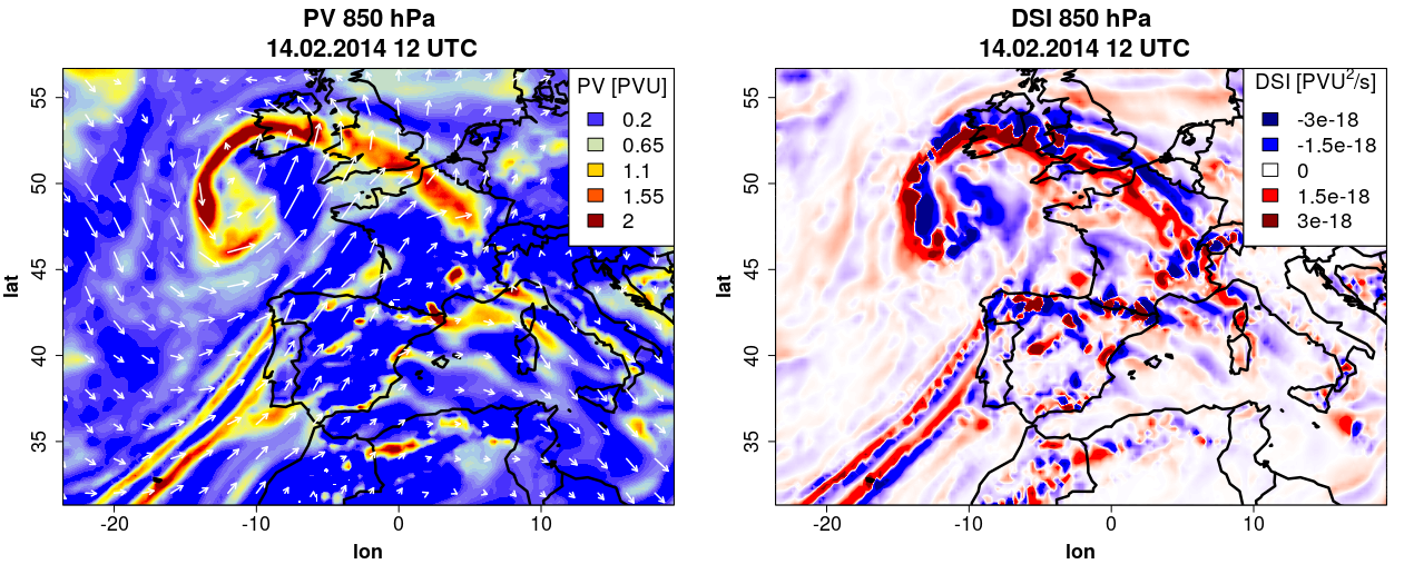
Figure 6: Left: Potential vorticity (coloured) and horizontal wind (white arrows) both at 850 hPa. Right: DSI at 850 hPa.

Gaßmann, (2014) showed that at least in the horizontal the stationary wind can be approximated by the real wind. Consequently, a zonal wind crossing a cyclonic PV anomaly leads to positive values upstream (due to $\nabla\Pi^{2}>0$) and negative values downstream (due to $\nabla\Pi^{2}<0$). Thus, frontal zones are characterized by large $|DSI|$ values. Müller et al., (2018) showed that the structure of frontal rain bands is reflected in the DSI. Based on time series analysis, Claussnitzer and Névir, (2009) and Claussnitzer, (2010) demonstrated that $|DSI|$ shows a high correlation with precipitation sums. Moreover, von Lindheim et al., (2021) showed that the DSI is associated with persistent and coherent structures in atmospheric flows like fronts. All these properties make the DSI a suitable tool to identify diabatically active fronts. For this purpose, we have developed the following algorithm:

  Algorithm 3: Front identification using DSI (”DSI method”)   front lines

front locator: $$\|\nabla_{h}DSI\|\cdot\frac{\nabla_{h}\Pi}{\|\nabla_{h}\Pi\|}=0$$ (22)

masking: $$DSI<q_{p_{1}}(DSI)\;\quad\quad\quad\>\rightarrow\textrm{negative values, e.g. }p_{1}=10\>\%$$ (23)

  frontal zones

masking: $$|DSI|>q_{p_{2}}(DSI)\quad\rightarrow\textrm{positive values, e.g. }p_{2}=95\>\%$$ (24)

 

For the front locator, we consider the gradient of the DSI projected onto the unit vector of the PV. This is inspired by the TFP method (Eq. 3), but in contrast to the unit vector of the thermic quantity we use the unit vector of the PV, which always points in the direction of the frontal zone and consequently allows us to outline the whole frontal zone (front and back side). In order to filter out only the front line, the DSI must have particularly negative values, which can be measured by using a small percentile (masking Eq. 23). As figure 7 shows, the occlusion front, the warm front and the ana cold front are detected in the case study. Compared to the TFP method, the cold front line is more interrupted, and in contrast to the F diagnostic, the entire warm front is detected.
Frontal zones are detected by particularly high values of the magnitude of the DSI (Eq. 24). This is different from the TFP method, where only the positive values (and not the absolute values) are used to capture frontal zones. We determine the threshold values using height-dependent percentiles. This has the advantage to avoid a height bias due to the increase of PV (and consequently also DSI) with height. Also, using a percentile allows to adjust the sensitivity of our method.

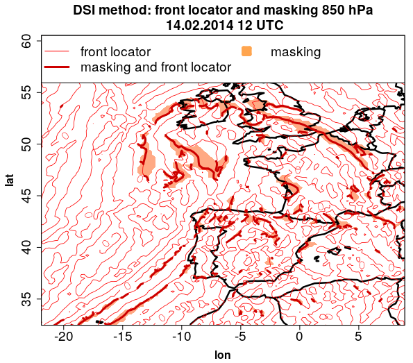
Figure 7: DSI method: Front locator (thin red lines), masking condition (orange shading) and the intersection of both (thick red lines) at 850 hPa, 14.02.2014 12 UTC.

4 Comparison of the front identification methods

In this chapter, we compare the three methods for front identification (TFP, F diagnostic and DSI) spatially and temporally. As the F diagnostic only allows the detection of frontal zones, we consider them only and refer to them as ”fronts” for the sake of simplicity. In the end, we examine the essential characteristics of the respective detected fronts. For this purpose, we consider mid-level fronts at 600 hPa. Using 850 hPa (as shown before) is unfavorable not only due to strong orography influence but also due to the influence of the boundary layer, which itself is strongly influenced by the land-sea contrast and the sea surface temperature (e.g., Parfitt et al., (2016)).

4.1 Climatology

Fig. 8 shows the occurrence probability of detected fronts (global north winter climatology, i.e. DJF 2000-2019, based on hourly data with a resolution of 0.25^∘$\times$0.25^∘) using the three previously described methods. The TFP method detects the northern hemisphere Atlantic and Pacific storm tracks, which are partly washed out to the north. The southern hemisphere (summer) storm tracks are also recognizable in lower intensity. The F diagnostic (using the recommended threshold $F>2$ for mid-level fronts) shows strong signals along the northern hemisphere storm tracks, but only weak signals along the southern hemisphere storm tracks. The region around the equator is masked out due to the convergence of the Coriolis parameter (as recommended by Parfitt et al., (2017)). Also the DSI method detects clearly the northern hemisphere storm tracks with their typical characteristics (northward tilt and eastward intensity decrease (Hoskins and Hodges, , 2002)) and as well the southern hemisphere storm tracks in a stronger intensity then the F diagnostic. Compared to the TFP method the southern hemisphere storm tracks detected by the DSI method are more pronounced over the Atlantic and Indian Ocean, which is consistent with the cyclogenesis density found by Hoskins and Hodges, (2005). All methods show also signals along the inner tropical convergence zone.

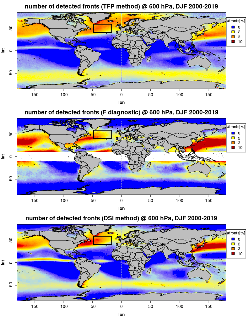
Figure 8: Front Climatology: Number of detected fronts (measured as occurrence probability) for twenty north winters (DJF 2000-2019) using TFP method (top), F diagnostic (middle) and DSI method with 95 % percentile (bottom).

4.2 Annual cycle

In order to quantitatively compare the annual variation of the determined number of fronts with the three methods and to avoid bias due to orography, only a box (shown in Fig. 8) over the North Atlantic is used. The annual cycle of the detected fronts at 600 hPa over this North Atlantic box with the TFP method, the F diagnostic and the DSI method for the three percentiles 95 %, 97 %, and 99 %, respectively is shown in Fig. 9. Here, ten years from 2010 to 2019 (each day 0 UTC) were considered. With the TFP method, more fronts are recorded in winter (maximum in January) than in summer (minimum in July). The general fact that fewer fronts are recorded in summer than in winter can be explained by the northward shift of the storm tracks, while the considered box remains fixed. Second, regardless of the area considered baroclinicity, mean wind speed and thus relative vorticity are on average weaker in summer than in winter (e.g., Hoskins and Hodges, (2002)). Also with the F diagnostic more fronts are detected in winter (maximum in February) than in summer (minimum in August). The difference between minimum and maximum is larger with F diagnostic than with all other methods, which can be explained by the fact that both baroclinicity and relative vorticity are higher on average in winter than in summer, and using their product in the F diagnostic then overemphasizes this difference. With the DSI method, more fronts are recorded in winter than in summer for all three percentiles, as well. The maximum number of fronts is reached in January for all percentiles, the minimum already in May, then the number of fronts increases slightly until another local minimum is reached in August. The summer-winter spread is not so pronounced with the DSI method. If higher percentiles are used for filtering, fewer fronts are recorded and the difference between summer and winter decreases further. The fact that more fronts are recorded with the DSI method in summer than with the other methods is possibly due to the construction of the DSI. Regardless of the amount of baroclinicity itself, fronts represent a deviation from the basic state in every season. Additionally, the availability of moisture for diabatic processes is larger in summer due to higher temperatures (this will be considered in the next sub chapter).

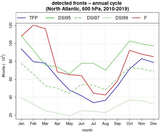
Figure 9: Annual cycle of detected fronts: Average number of detected fronts per month using TFP method, F diagnostic and DSI method (percentiles 95 %, 97 % and 99 %, respectively) at 600 hPa over the North Atlantic between 2010-2019.

4.3 Properties of the detected fronts

Fig. 10 shows the distribution of specific humidity, baroclinicity measured by $\|\nabla_{h}T\|$ and relative vorticity of the fronts detected with the TFP method, the F diagnostic and the DSI method (95 % percentile), respectively. Fronts detected with the DSI method are characterized by high specific humidity. Because the DSI measures diabatic processes for which humidity is a prerequisite, this seems reasonable. Fronts detected with the TFP method show high baroclinicity (due to the definition of the TFP) and anticylonic vorticity in average. The latter is not reasonable as fronts are associated with lows and itself are areas of high relative vorticity. Fronts detected with the F diagnostic are characterized by high baroclinicity and high relative vorticity (both due to the definition of F) but low specific humidity. These results show that for investigating fronts in general, like Spensberger and Sprenger, (2018), it has to be checked whether the results are robust regarding the used method. Furthermore, this confirms the results of Soster and Parfitt, (2022), who investigated how precipitation can be assigned to fronts and how this depends on the method and reanalysis used. They have shown that when using the TFP method, on average less precipitation is associated with fronts than when using the F diagnostic. Our results now suggest that this is due to the lack of a vortical dynamic component in the TFP procedure, which leads to many ”fronts” with anticyclonic vorticity, i.e., passing through areas of high pressure.

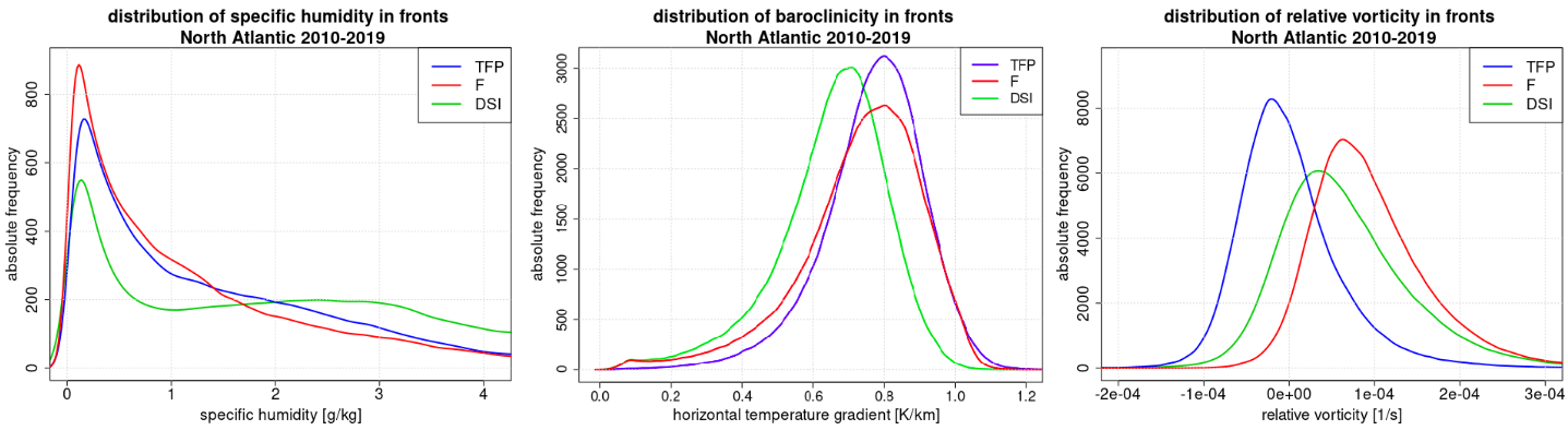
Figure 10: Front properties: Distribution of specific humidity, baroclinicity and relative vorticity in the respective detected fronts (TFP method, F diagnostic, DSI method with 95 % percentile) at 600 hPa over the North Atlantic between 2010-2019.

Following Hewson, (1998), the movement speed of front lines, determined as contours of a quantity $\Psi$, can be estimated by

$$v_{f}=\boldsymbol{v}_{h}\cdot\frac{\nabla_{h}\Psi}{\|\nabla_{h}\Psi\|}=\boldsymbol{v}_{h}\cdot\boldsymbol{e}_{\Psi}\leq\|\boldsymbol{v}_{h}\|.$$ (25)

The horizontal wind $\boldsymbol{v}_{h}$ is projected onto the horizontal unit vector $\boldsymbol{e}_{\Psi}$, so that the maximum front speed is constrained by $\|\boldsymbol{v}_{h}\|$. Since Eq. 25 considers the displacement of contours (and not surfaces), the front speed is calculated only for the TFP method ($\Psi=TFP$) and the DSI method ($\Psi=DSI$). The average front speed in the North Atlantic box using the TFP method is 12,6 m/s in winter and 9,5 m/s in summer, while using the DSI method it is 17,1 m/s in winter and 13,8 m/s in summer (both normalized with the respective number of fronts detected). Since the selected quantity $\Psi$ enters the calculation of the speed of movement only via the unit vector (i.e. as a direction and not as magnitude), it can be deduced that $\boldsymbol{e}_{DSI}$ is on average ”more parallel” to $\boldsymbol{v}_{h}$ than $\boldsymbol{e}_{TFP}$. This confirms the capacity of the DSI to indicate the direction of movement (see, Fig. 6).

5 Summary and conclusions

This paper has discussed different methods to identify fronts in ERA5 reanalysis. We have examined how secondary vortex dynamic quantities affect front identification and the properties of the detected fronts.
First, we have discussed two state-of-the-art methods for identifying fronts, the TFP method and the F diagnostic. The TFP method allows for the detection of both front lines and frontal zones, while the F diagnostic only allows the detection of frontal zones but with a lower order, as summarized in Tab. 1. While the TFP is a purely thermal quantity, the F diagnostic combines a thermal and a vortex dynamic quantity. If not only the TFP but also the baroclinicity is used as masking condition in the TFP procedure, weak warm fronts are unintentionally not detected. Therefore, we have omitted this second masking step. The F diagnostic also fails to detect weak warm fronts or detects them only partially, while the low center is misidentified as a front due to the combination of baroclinicity and vorticity. But this problem can possibly be circumvented by using more appropriate thresholds. By considering that the F diagnostic contains the Rossby number we have provided a new way to interpret the F diagnostic as a baroclinicity-weighted measure of spatial scale.
We have developed a new front identification method that considers fronts as a deviation from a stationary, inviscid and adiabatic basic state. This deviation is measured by the DSI. The DSI method allows the detection of front lines and frontal zones using percentile exceedances. This makes this method adaptable and independent of altitude. We have shown that the DSI method clearly identifies the storm track regions on both hemispheres. In contrast to the other methods, the number of fronts detected with the DSI method varies less during the year. The fronts detected with the F diagnostic show the largest spread between winter maximum and summer minimum, again due to the combination of baroclinicity and vorticity, which are positively correlated in frontal zones due to transverse circulation (Hoskins, , 1982; Parfitt et al., , 2017).

method	quantities	frontal zones ($\mathcal{O}$)	frontal lines ($\mathcal{O}$)	properties of detected fronts
TFP	$\theta$	yes (2)	yes (3)	baroclinicity
F	$T,\>\zeta$	yes (1)	no	baroclinicity, vorticity
DSI	$\theta,B,\Pi$	yes (2)	yes (3)	specific humidity

Table 1: Properties of the compared front identification methods: Contained quantities, features of the methods ($\mathcal{O}$ represents the order) and properties of the respective detected fronts.

Comparing the properties of the respective detected fronts, we have found that fronts identified using TFP method show high baroclinicity but in average anticyclonic relative vorticity. The ones identified with F diagnostic show high baroclinicity and high relative vorticity and the ones identified with the DSI method show high specific humidity. On the one hand, this indicates that the properties of the detected fronts strongly depend on the method used, which is consistent with the results of Soster and Parfitt, (2022), who investigated the allocation of precipitation to fronts. On the other hand, it also demonstrates the potential of the DSI method to identify diabatic active fronts associated with high humidity and the potential for heavy rain.
Using a simple estimate for the speed of movement of fronts introduced by Hewson, (1998), we have shown that the front speed is smaller for the TFP method than for the DSI method. This shows the potential of the DSI method to indicate the direction of motion of meteorological objects, which should be investigated more in detail in future studies. Moreover, the novel DSI method can further be applied to investigate the global distribution of diabatic active fronts and their relationship to (extreme) precipitation.

References

- Berry et al., (2011) Berry, G., Reeder, M. J., and Jakob, C. (2011). A global climatology of atmospheric fronts. Geophys. Res. Lett., 38(L04809).
- Bjerknes and Solberg, (1922) Bjerknes, J. and Solberg, H. (1922). Life cycle of cyclones and the polar front theory of atmospheric circulation. Geofys. Publ., 3(1):3–18.
- Bott, (2016) Bott, A. (2016). Synoptische Meteorologie: Methoden der Wetteranalyse und -prognose. Springer Spektrum Verlag, Berlin, Heidelberg.
- Catto et al., (2012) Catto, J. L., Jakob, C. L., Berry, G., and Nicholls, N. (2012). Relating global precipitation to atmospheric fronts. Geophys. Res. Lett., 39(L10805).
- Catto and Pfahl, (2013) Catto, J. L. and Pfahl, S. (2013). The importance of fronts for extreme precipitation. J. Geophys. Res. Atmos., 118:10791–10801.
- Claussnitzer, (2010) Claussnitzer, A. (2010). Statistisch-dynamische Analyse skalenabhängiger Niederschlagsprozesse: Vergleich zwischen Beobachtungen und Modell. PhD thesis, Freie Universität Berlin.
- Claussnitzer and Névir, (2009) Claussnitzer, A. and Névir, P. (2009). Analysis of quantitative precipitation forecasts using the Dynamic State Index. Atmos. Res., 94(4):694–703.
- Claussnitzer et al., (2008) Claussnitzer, A., Névir, P., Langer, I., Reimer, E., and Cubasch, U. (2008). Scale-dependent analyses of precipitation forecasts and cloud properties using the Dynamic State Index. Meteorol. Z., 17(6):813–825.
- Gaßmann, (2014) Gaßmann, A. (2014). Deviations from a general nonlinear wind balance: Local and zonal-mean perspectives. Meteorol. Z., pages 467–481.
- Gassmann, (2019) Gassmann, A. (2019). Analysis of large-scale dynamics and gravity waves under shedding of inactive flow components. Monthly Weather Review, 147(8):2861–2876.
- Grazzini et al., (2020) Grazzini, F., Craig, G., Keil, C., Antolini, G., and Pavan, V. (2020). Extreme precipitation events over northern Italy. Part I: a systematic classification with machine-learning techniques. Quart. J. Roy. Meteor. Soc., 146:69–85.
- Hersbach et al., (2020) Hersbach, H., Bell, B., Berrisford, P., Hirahara, S., Horányi, A., Muñoz-Sabater, J., et al. (2020). The ERA5 global reanalysis. Quart. J. Roy. Meteor. Soc., 146:1999–2049.
- Hewson, (1998) Hewson, T. D. (1998). Objective fronts. Meteorol. Appl., 5:37–65.
- Hoskins, (1982) Hoskins, B. J. (1982). The mathematical theory of frontogenesis. Annu. Rev. Fluid Mech., 14(1):131–151.
- Hoskins and Hodges, (2002) Hoskins, B. J. and Hodges, K. I. (2002). New perspectives on the Northern Hemisphere winter storm tracks. J. Atmos. Sci., 59(6):1041–1061.
- Hoskins and Hodges, (2005) Hoskins, B. J. and Hodges, K. I. (2005). New perspectives on Southern Hemisphere winter storm tracks. Journal of Climate, 18:4108–4129.
- Huber-Pock and Kress, (1981) Huber-Pock, F. and Kress, C. (1981). Contributions to the problem of numerical frontal analysis. Proceedings of the Symposium on Current Problems of Weather-Prediction. Vienna, June 23–26, 1981. Publications of the Zentralanstalt für Meteorologie und Geodynamik, 253.
- Kern et al., (2019) Kern, M., Hewson, T., Schäfler, A., Westermann, R., and Rautenhaus, M. (2019). Interactive 3D Visual Analysis of Atmospheric Fronts. IEEE Transactions on Visualization and Computer Graphics, 25(1).
- Müller et al., (2018) Müller, A., Névir, P., and Klein, R. (2018). Scale dependent analytical investigation of the dynamic state index concerning the quasi-geostrophic theory. Mathematics of Climate and Weather Forecasting, 4(1):1–22.
- Névir, (2004) Névir, P. (2004). Ertel’s vorticity theorems, the particle relabelling symmetry and the energy-vorticity theory of fluid mechanics. Meteorol. Z., 13(6):485–498.
- Parfitt et al., (2016) Parfitt, R., Czaja, A., Minobe, S., and Kuwano-Yoshida, A. (2016). The atmospheric frontal response to SST perturbations in the Gulf Stream region. Geophys. Res. Lett., 43:2299–2306.
- Parfitt et al., (2017) Parfitt, R., Czaja, A., and Seo, H. (2017). A simple diagnostic for the detection of atmospheric fronts. Geophys. Res. Lett., 44:4351–4358.
- R Core Team, (2020) R Core Team (2020). R: A Language and Environment for Statistical Computing.
- Raveh-Rubin and Catto, (2019) Raveh-Rubin, S. and Catto, J. L. (2019). Climatology and dynamics of the link between dry intrusions and cold fronts during winter, Part II: Front-centred perspective. Climate Dynamics, 53:1893–1909.
- Renard and Clarke, (1965) Renard, R. J. and Clarke, L. C. (1965). Experiments and numerical objective frontal analysis. Monthly Weather Review, 93:547–556.
- Schär, (1993) Schär, C. (1993). A generalization of Bernoulli’s theorem. J. Atmos. Sci., 50(10):1437–1443.
- Shapiro and Keyser, (1990) Shapiro, M. A. and Keyser, D. (1990). Fronts, jet streams and the tropopause. Extratropical Cyclones: The Erik Palmén Memorial Volume, C. Newton and E.O. Holopainen, Eds., Amer. Meteor. Soc., pages 167–191.
- Solari et al., (2022) Solari, F. I., Blásquez, J., and Solman, S. A. (2022). Relationship between frontal systems and extreme precipitation over southern South America. International Journal of Climatology.
- Soster and Parfitt, (2022) Soster, F. and Parfitt, R. (2022). On Objective Identification of Atmospheric Fronts and Frontal Precipitation in Reanalysis Datasets. Journal of Climate, 35:4513–4534.
- Spensberger and Sprenger, (2018) Spensberger, C. and Sprenger, M. (2018). Beyond cold and warm: an objective classification for maritime midlatitude fronts. Q. J. R. Meteorol. Soc., 144:261–277.
- Thomas and Schultz, (2019) Thomas, C. M. and Schultz, D. M. (2019). Global Climatologies of Fronts, Airmass Boundaries, and Airstream Boundaries: Why the Definition of ”Front” Matters. Mon. Wea. Rev., 147:691–717.
- Uccellini et al., (1992) Uccellini, L. W., Corfidi, S. F., Junker, N. W., Kocin, P. J., and Olson, D. (1992). Report on the surface analysis workshop held at the National Meteorological Center 25-28 March 1991. Bull. Amer. Meteor. Soc., 73:459–471.
- Volonté et al., (2018) Volonté, A., Clark, P. A., and Gray, S. L. (2018). The role of mesoscale instabilities in the sting-jet dynamics of windstorm Tini. Q. J. R. Meteorol. Soc., 144:877–899.
- von Lindheim et al., (2021) von Lindheim, J., Harikrishnan, A., Dörffel, T., Klein, R., Koltai, P., Mikula, N., Müller, A., Névir, P., Pacey, G., Polzin, R., and Vercauteren, N. (2021). Definition, detection, and tracking of persistent structures in atmospheric flows. arXiv:2111.13645.
- Weber and Névir, (2008) Weber, T. and Névir, P. (2008). Storm tracks and cyclone development using the theoretical concept of the Dynamic State Index (DSI). Tellus A, 60(1):1–10.