Study of Low-dimensional Nonlinear Fractional Difference Equations of Complex Order

Abstract

We study the fractional maps of complex order, $\alpha_{0}e^{ir\pi/2}$ for $0<\alpha_{0}<1$ and $0\leq r<1$ in 1 and 2 dimensions. In two dimensions, we study Hénon and Lozi map and in $1d$, we study logistic, tent, Gauss, circle, and Bernoulli maps. The generalization in $2d$ can be done in two different ways which are not equivalent for fractional-order and lead to different bifurcation diagrams. We observed that the smooth maps such as logistic, Gauss, and Hénon maps do not show chaos while discontinuous maps such as Lozi, Bernoulli, and circle maps show chaos. The tent map is continuous but not differentiable and it shows chaos as well. In $2d$, we find that the complex fractional-order maps that show chaos also show multistability. Thus, it can be inferred that the smooth maps of complex fractional-order tend to show more regular behavior than the discontinuous or non-differentiable maps.

Complex differential equations of real fractional order or differential equations of complex fractional order have been studied in the context of some applications. We study the dynamics of difference equations of complex fractional order. In general, the right-hand side of these equations involves arbitrary functions. We find that for a highly restrictive set of functions, i.e., complex analytic functions, no chaos is observed in dynamics. The variables can be extended to complex space by using complex initial conditions even for real fractional order. We observe that complex difference equations of real fractional order do not show any chaos for complex analytic functions either.

I Introduction

Though studies in fractional calculus started from Leibniz and almost all leading mathematicians have contributed to its theory, it has received tremendous attention in the last few decades. Fractional versions of several differential equations have been investigated numerically as well as analytically. These studies are mostly related to real fractional-order differential equations. It has found several applications in the recent past in fields as diverse as heat transfer equations and viscoelasticity and is an active area of research francisco2014fractional ; oprzkedkiewicz2021fractional ; meral2010fractional . A natural curiosity is whether we can obtain a derivative of imaginary order and Love can be credited for defining it for the first time love1971fractional . This was later extended to arbitrary complex order andriambololona2012definitions ; campos1990solution . Unlike real fractional order differential equations, applications of complex fractional order differential equations are not so well established. Makris and Constantinou suggested applications in viscoelasticity makris . Makris also gave a complex parameter Kevin model for elastic foundations makris2 . The boundary value problem for fractional differential equation of complex order is studied in nea . As noted in ortigueira2021complex , a major difficulty with complex derivatives is that it treats positive and negative frequencies differently and the sum or difference of complex order derivative and its conjugate has been proposed as one of the solutions adams ; atanackovic2015vibrations . Still, the complex order fractional derivatives can be quite attractive from the application point of view. As stated by Makris, "Complex-parameter models are very attractive, because a minimum number of parameters is required to obtain a satisfactory fit of the ‘exact’ response. For instance, in modeling the response of a rigid disc resting on elastic foundations, only two complex-valued frequency-independent parameters are sufficient to reproduce closely the rigorously obtained dynamic stiffness for the vertical, horizontal, and rocking modes" makris3 . Atanovic and Pilipovic studied heat conduction with a general form of a constitutive equation containing a fractional derivative of real and complex order atanackovic2018constitutive .

From the viewpoint of control, fractional order controllers are found to be effective and complex order controllers have also been used. It is obvious that complex order operators produce complex-valued output even for a real-valued function and hence it was proposed that a complex-order operator should be paired with conjugate order operatorHartley . Tare et al. designed complex-order PID controller structures using conjugated order derivatives. The model was comparatively studied and found to have an overall better performance owing to its more flexible structure tare2019design . Sekhar et al studied complex order controller where they simply omitted the imaginary part of derivative as well as complex integrationsekhar2020complex . Another interesting application of complex order derivative has been particle swarm optimizationpahnehkolaei2021particle .

Nonlinear dynamics of continuous-time complex order fractional systems has also received some attention. Pinto has studied the dynamics of two unidirectional rings of cells coupled through a buffer cellpinto2015strange . Applications of complex order derivative have been studied in animal locomotionpinto2011complex . The theory of hybrid fractional differential equations with complex order has been developed in vivek2019theory . In pinto , Pinto and Carvalho studied the fractional complex order model for HIV infection. Variation of complex order sheds light on the modeling of intracellular delay and the model offers rich dynamics. Pinto and Machado studied complex order van der Pol oscillator and complex order forced van der Pol oscillator pinto2 ; pinto3 .

The introduction of a complex-order fractional derivative leads to complex-valued variables even if initial conditions are real. We may also study the dynamics of complex fractional differential equations where the real fractional-order derivative is employed. There are several works in this context. Chaos synchronization, as well as control, has been observed in fractional-order complex, chaotic systems, and it has been studied in singh2017synchronization ; luo2013chaos ; gao2005chaos . In all these works, we observe that the functions are functions of the variables as well as their conjugates. Thus, these are not analytic functions and they are effectively real dynamical systems with double the dimension. It would be interesting to study the possibility of chaos if we insist that the functions should be analytic. We explore this question in the context of discrete maps by studying several systems.

Discrete maps have played a major role in understanding dynamical systems. Simulations of discrete maps are easier computationally. Several phenomena that appear in flows occur in maps as well ott . Thus, understanding discrete maps can complement our understanding of flows. Many control schemes useful for the control of differential equations can be used for maps as well shinbrot1993using .

While we need at least a three-dimensional continuous-time system to observe chaos, it can be observed even in one-dimensional difference equations. The most-studied maps in this context are logistic and tent maps. The question is whether this feature is retained in presence of memory and studies in fractional difference equations are important in this context. The studies in fractional difference equations are relatively recent holm2011theory ; atici2009initial ; atici2007transform ; atici2012gronwall . There have been studies on the stability of fractional difference equations and in recent times, the definition is extended to complex orders gade2021fractional ; bhalekar2022stability . In particular, the stability conditions for linear fractional difference equations of complex order have been derived bhalekar2022stability . For this scheme, linear systems have been studied in gade2021fractional and it is known that the trajectories that converge to origin converge as a Mittag-Leffler function which is a power-law asymptotically. On the other hand, unstable trajectories diverge exponentially. Thus, positive Lyapunov exponent can be used to quantify chaos in these systems. It is of interest to explore the possibility of chaos in genuinely complex maps in any dimension, where the functions are analytic functions of variables and do not involve their complex conjugates.

We briefly review prototypical and well-studied systems in discrete dynamics. The logistic map and tent map in $1d$ show chaos and have been extensively studied in this context. The maps, such as the circle map, model dynamical systems represented by the damped driven pendulum such as Josephson junction in the microwave field, charge density waves, lasers, and even air-bubble formation bohr1984transition ; tredicce1985instabilities ; detienne1997semiconductor ; tufaile2001circle . Gauss map has domain over $\mathbb{R}$, unlike other maps. The Bernoulli map is easy to study analytically. These maps have been studied by several researchers. In $2d$, the Hénon map and Lozi map are popular and well-investigated maps. We study the extension of these $1d$ and $2d$ maps to fractional complex orders. These systems can be classified into a few different categories. Logistic map, Hénon map, and Gauss map are continuous and differentiable. Bernoulli, circle, and Lozi maps are discontinuous. The tent map is continuous but not differentiable. The key finding is that continuous and differentiable maps do not show chaotic attractors for complex fractional orders. If there is chaos for real fractional order at a certain parameter value, the trajectories blow up and the system is no longer bounded if we turn on complex order. We will demonstrate these findings on a case-by-case basis below. The extension to complex orders for discontinuous systems is not straightforward since the underlying variables become complex and effectively two-dimensional. We have chosen certain rules for extending the map to complex order. However, other generalizations are possible.

a) Gauss map: The Gauss map is defined as

$$x_{n+1}=\exp{(-\nu x^{2}_{n})}+\beta,$$

where $\nu$ and $\beta$ are the parameters. The parameter $\nu$ is fixed and $\nu=7.5$. The parameter $\beta$ lies between [-1,1]
b) Logistic map: This map is given as

$$x_{n+1}=\lambda x_{n}(1-x_{n}),$$

where $\lambda$ is a parameter that lies between [0,4].
c)Circle map: The circle map is given as

$$x_{n+1}=x_{n}+\Omega-\frac{K}{2\pi}\sin(2\pi x_{n})|(mod\;1).$$

Here $x_{n+1}$ is computed ($mod\;1$) and $K$ is a constant. We fix the value of $\Omega=0.6$ for the rest of the paper. In our simulations, $K$ lies between [0,5.5].
d)Bernoulli map: The Bernoulli map is defined as

$$x_{n+1}=px_{n}|(mod\;1).$$

Here, $p$ lies between [0,2]
e)Tent map is a piecewise linear map defined as

$$x_{n+1}=\begin{cases}\mu x_{n},&|x_{n}|<\frac{1}{2},\\ \mu(1-x_{n}),&|x_{n}|>\frac{1}{2}.\end{cases}$$

In this map, the absolute value of the local slope is always $\mu$ and it lies between [0,2].

In integer-order difference equations, the dynamics of two-dimensional maps is much richer than one-dimensional maps. Lorenz system was one of the earliest systems of differential equations where chaos was seen lorenz1963deterministic . Hénon introduced a simple two-dimensional map that showed similar characteristics. The Hénon map is a two-dimensional invertible iterated map with squared nonlinearity and strange attractor chaotic solutions. In 1976, Michel Hénon, henon1976two , introduced this map given as

$$x_{n+1}=1+y_{n}-ax^{2}_{n}$$

$$y_{n+1}=bx_{n}.$$

This is one of the earliest and most studied maps elhadj2013lozi . It has a contraction rate that is independent of the values of variables. It reduces to a well-known logistic map for $b=0$. Over a certain range of parameter values, it has bounded solutions and it shows chaos at some of the values. Hénon carried out numerical experiments and obtained a strange attractor for $a=1.4$ and $b=0.3$. However, most of the properties are known only numerically, and hence Lozi introduced a new map that is hyperbolic, ergodic, and easier to study analytically in 1978 lozi1978attracteur . If the quadratic term in the Hénon map is replaced by the term $|x|$, we get the Lozi map. Thus, the Lozi map is given as

$$x_{n+1}=1+y_{n}-a|x_{n}|$$

$$y_{n+1}=bx_{n}.$$

The above maps are prototypical and well-studied in two dimensions. Naturally, extensions of these maps to fractional real order have been studied. There are more than one ways to introduce fractional maps. The fractional Hénon map was introduced in 2010 by Tarasov (See Ch. 1 of luo2011long ) and was later studied in liu2014discrete ; hu2014discrete . Fractional Hénon map in $3-d$ jouini2019fractional , and chaotic synchronization in fractional Hénon map liu2016chaotic has also been investigated. Fractional Lozi map is studied in khennaoui2019fractional and synchronization of fractional-order Lozi maps is considered in megherbi2017new . We extend these studies to complex fractional-order.

II Definition of Fractional maps

We study the maps mentioned above in complex fractional-order by using the definition of the fractional difference operator introduced in miller1988fractional ; atici2010modeling later extended to complex order bhalekar2022stability . The definition for the $1d$ nonlinear map is given as,

$$x(t)=x(0)+\frac{1}{\Gamma(\alpha)}\sum_{j=1}^{t}\frac{\Gamma(t-j+\alpha)}{\Gamma(t-j+1)}[f(x(j-1))-x(j-1)],$$ (1)

where, $f(x)$ is a nonlinear map as defined in a) to e). (The reason for subtracting the term $x(j-1)$ in the RHS of the above equation is to connect the discrete dynamical systems with difference equations as discussed in deshpande2016chaos ).

While extending the circle and Bernoulli map to the complex domain, we define the modulo function as follows. If $x=r\exp(\iota\theta)$ and $r>1$, we set $r_{new}=r-int[r]$ and $x=r_{new}\exp(\iota\theta)$.

For $2d$ maps, there are two possibilities. The Hénon map which is given by $x_{n+1}=1-ax_{n}^{2}+y_{n}$; $y_{n+1}=bx_{n}$ or an equivalent formulation is $x_{n+1}=1-ax_{n}^{2}+bx_{n-1}$. These two formulations are equivalent for integer-order maps. However, extending them to fractional-order leads to expressions that are not equivalent to each other. In the first case, we can formulate the fractional-order system as

$$x(t) = x(0)+\frac{1}{\Gamma(\alpha)}\sum_{j=1}^{t}\frac{\Gamma(t-j+\alpha)}{\Gamma(t-j+1)}$$

$$\times[1+y(j-1)-ax^{2}(j-1)-x(j-1)],$$

$$y(t) = y(0)+\frac{1}{\Gamma(\alpha)}\sum_{j=1}^{t}\frac{\Gamma(t-j+\alpha)}{\Gamma(t-j+1)}$$ (2)

$$\times[bx(j-1)-y(j-1)].$$

We denote this model as H2. In the second case, we can formulate

$$x(t)=x(0)+\frac{1}{\Gamma(\alpha)}\sum_{j=1}^{t}\frac{\Gamma(t-j+\alpha)}{\Gamma(t-j+1)}$$

$$\times\left[1+bx(j-2)-ax^{2}(j-1)-x(j-1)\right].$$ (3)

The formulation involving delay is used in liu2014discrete . We denote this model as H1. Some authors use the first definition hu2014discrete . (In fact, for the first definition, we can use different orders $\alpha$ and $\beta$ for the variables $x$ and $y$. However, we do not deal with such generalization in this work.) We could choose either formulation. The second formulation is computationally more efficient since it involves only one variable and could be a prototype for the delay system. We have carried out studies using both definitions in this work. We note that our major conclusions are not affected by this choice.

Similarly, we can formulate a fractional-order Lozi system either as

$$x(t) = x(0)+\frac{1}{\Gamma(\alpha)}\sum_{j=1}^{t}\frac{\Gamma(t-j+\alpha)}{\Gamma(t-j+1)}$$

$$\times[1+y(j-1)-a|x(j-1)|-x(j-1)]$$

$$y(t) = y(0)+\frac{1}{\Gamma(\alpha)}\sum_{j=1}^{t}\frac{\Gamma(t-j+\alpha)}{\Gamma(t-j+1)}$$ (4)

$$\times[bx(j-1)-y(j-1)],$$

or

$$x(t)=x(0)+\frac{1}{\Gamma(\alpha)}\sum_{j=1}^{t}\frac{\Gamma(t-j+\alpha)}{\Gamma(t-j+1)}$$

$$\times\left[1+bx(j-2)-a|x(j-1)|-x(j-1)\right],$$ (5)

where $\alpha$ is the order of the fractional difference operator. In our case, $\alpha$ is a complex number with $0<Re(\alpha)<1$. We denote models defined by eq(4) and (5) by model L2 and L1 respectively.

To systematically investigate the impact of complex order on fractional maps, we set $\alpha=\alpha_{0}e^{ir\pi/2}$ with $0<\alpha_{0}<1$ and $0\leq r<1$. It reduces to real fractional order for $r=0$.

III Dynamics and bifurcations for fractional-order maps

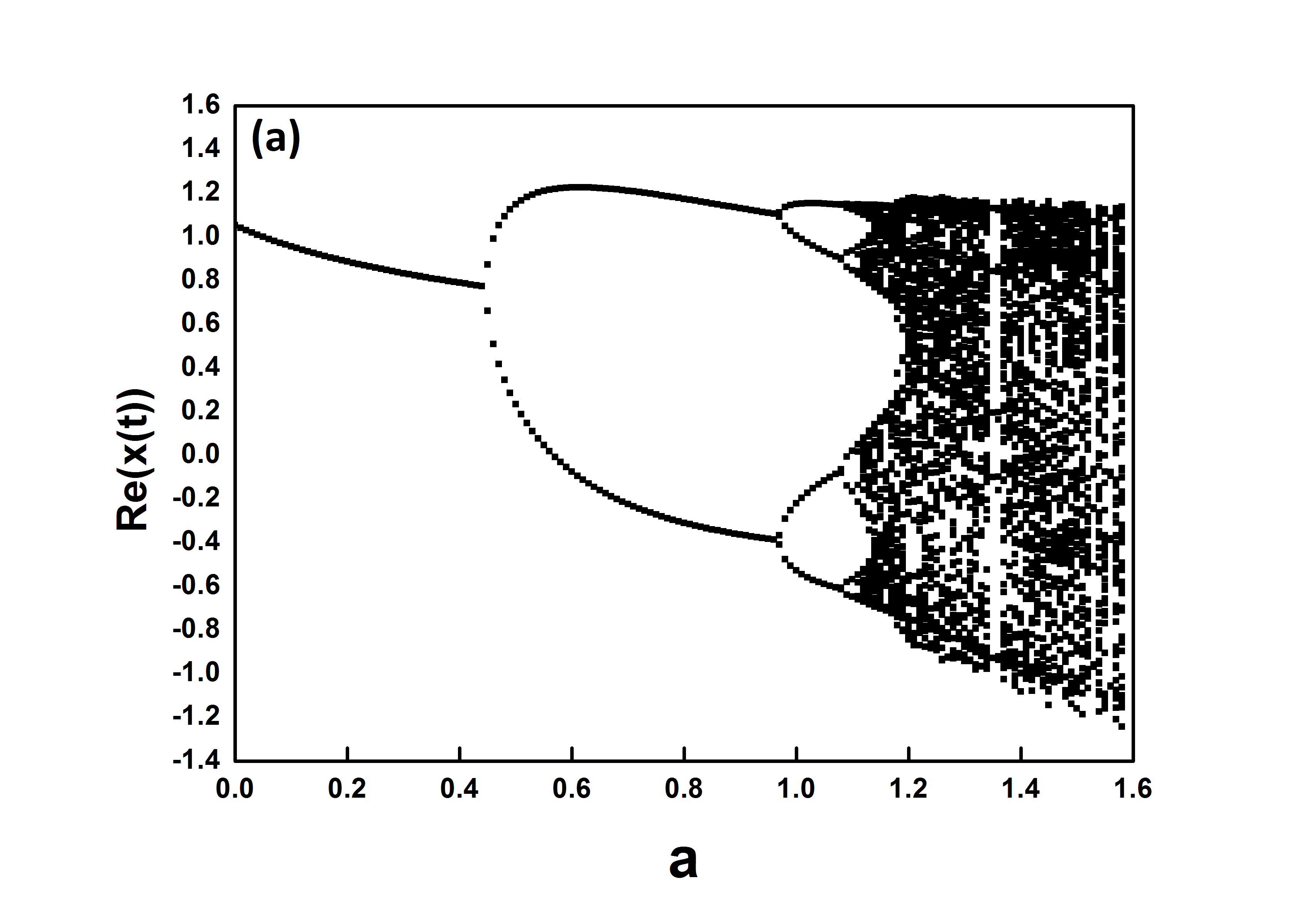
(a)

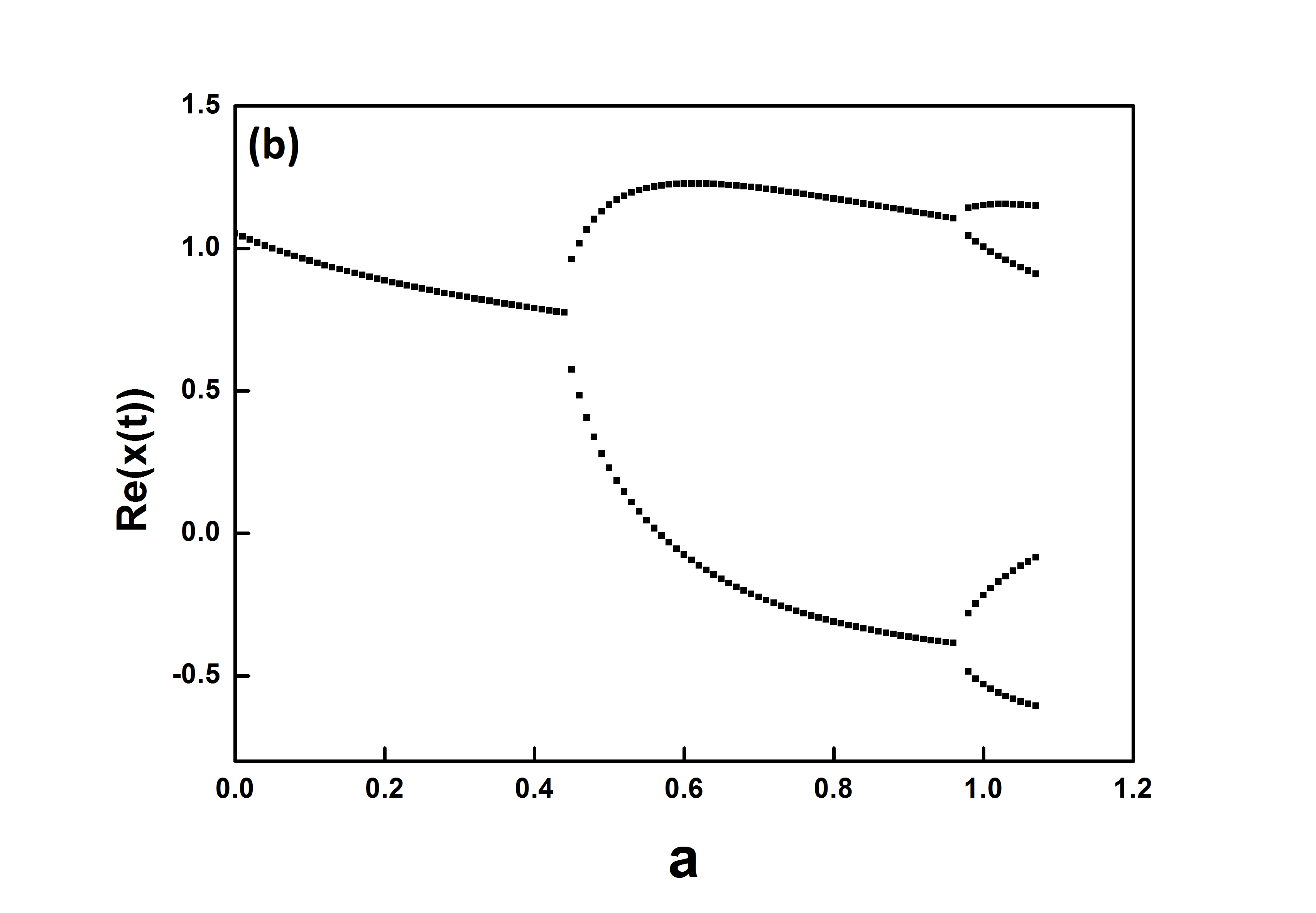
(b)

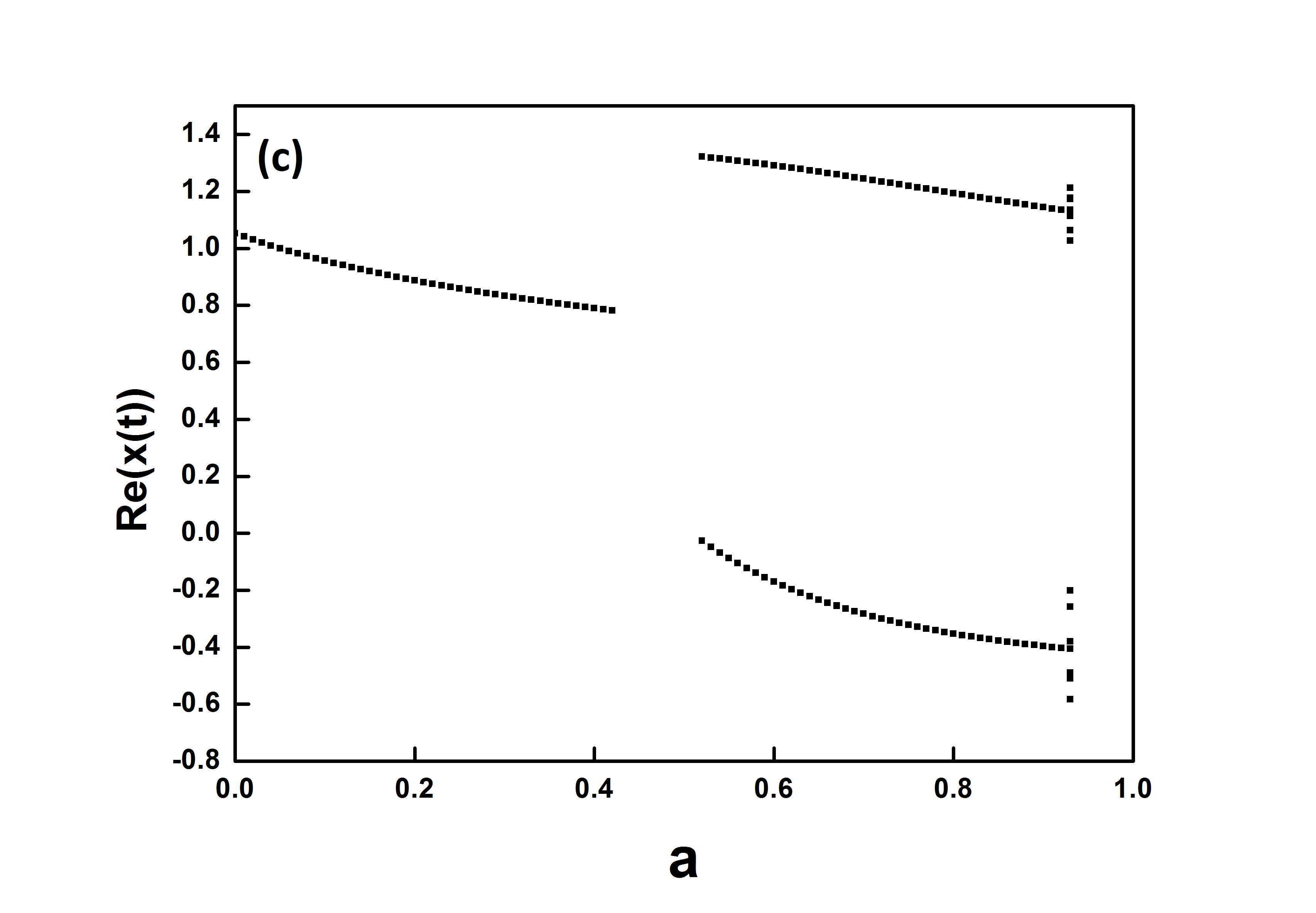
(c)

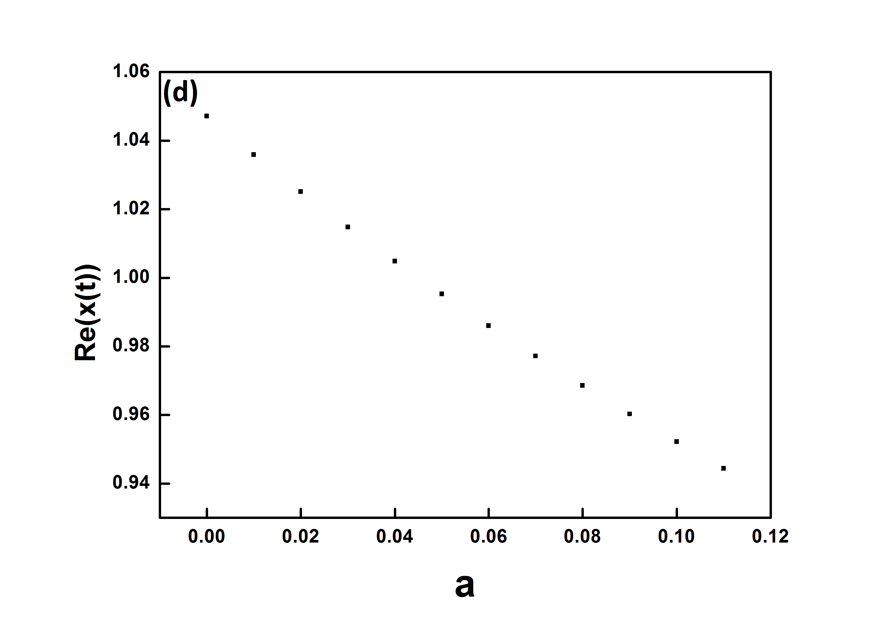
(d)

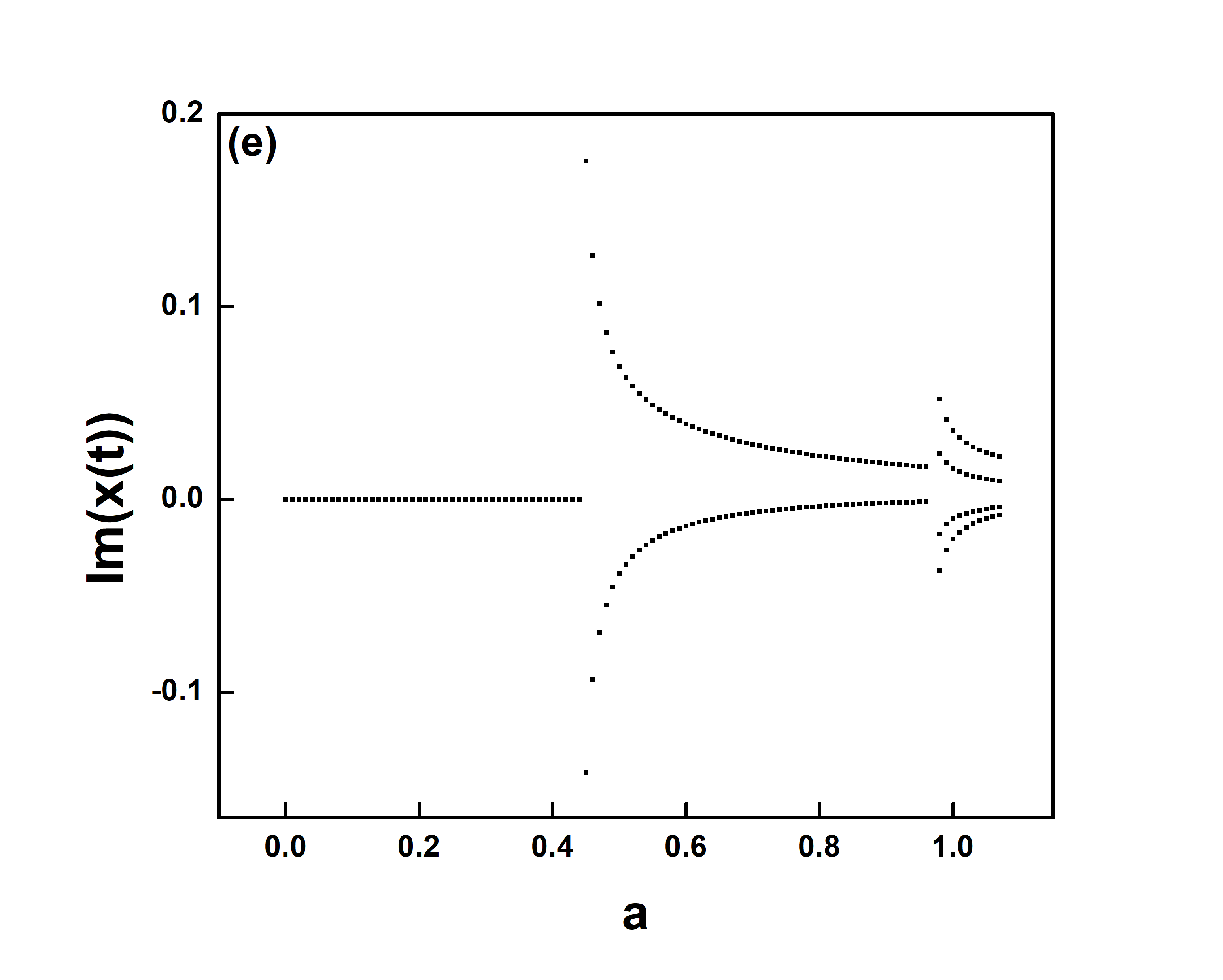
(e)

Figure 1: Bifurcation Diagrams($a$ vs $Re(x(t))$) for the Hénon map (model H1)for $b=0.05$ and $\alpha_{0}=0.8$ for (a)$r=0$, (b)$r=0.01$, (c)$r=0.1$, (d)$r=0.5$ and (e)$a$ vs $Im(x(t))$ for $\alpha_{0}=0.8,r=0.01$.

A powerful tool to understand the dynamics is a bifurcation diagram. The span of variable values is clear when we plot values of variables after a certain transient. At first, we see the bifurcation diagram for the Hénon map of order $\alpha=\alpha_{0}e^{ir\pi/2}$ as mentioned above. We have checked the values $\alpha_{0}=$ 0.1, 0.2, 0.3, 0.4, 0.5, 0.6, 0.7, 0.8, and 0.9. For all these values, we have checked the cases $r=$ 0, 0.01, 0.1, and 0.5 with initial condition $x(0)=y(0)=0$ for model H1. We do not observe chaos for $r\neq 0$ indicating that the chaotic attractor is destroyed when we introduce complex order. We have checked results with a few different initial conditions and the bifurcation diagram does not change indicating that multistability is not very pronounced for fractional-order.

We have shown the bifurcation diagram for $\alpha_{0}=0.8$ and $r=$ 0, 0.01, 0.1, and 0.5 in Figure (1). The chaos disappears even for small values of $r$. We have carried out the same exercise for model H2 and we do not observe a stable chaotic orbit with initial conditions $x(0)=y(0)=0$ for the cases mentioned above.

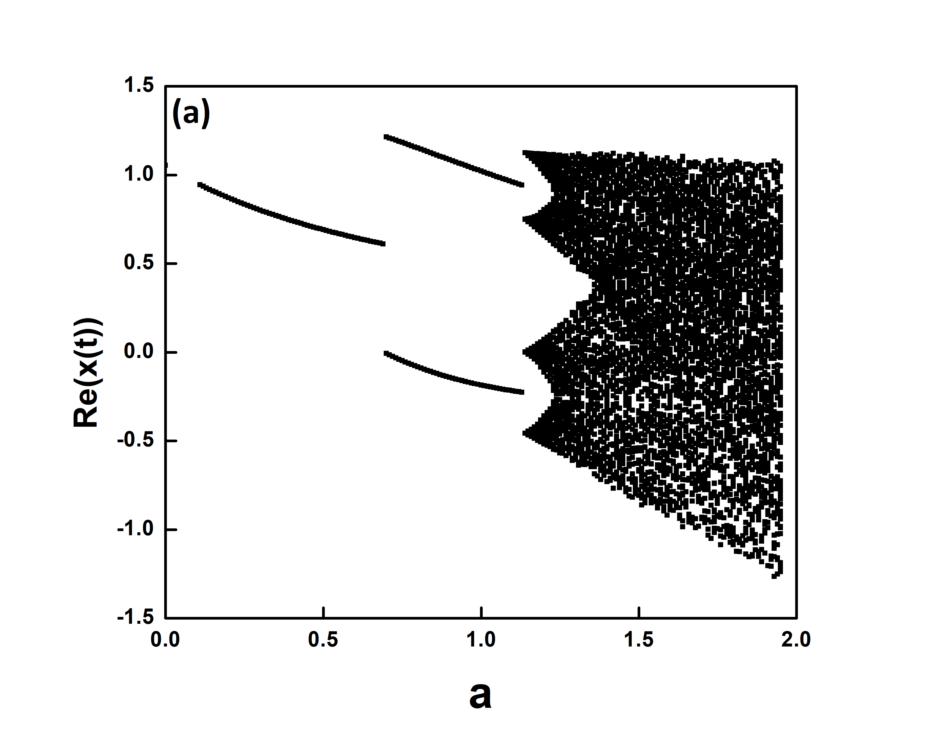
(a)

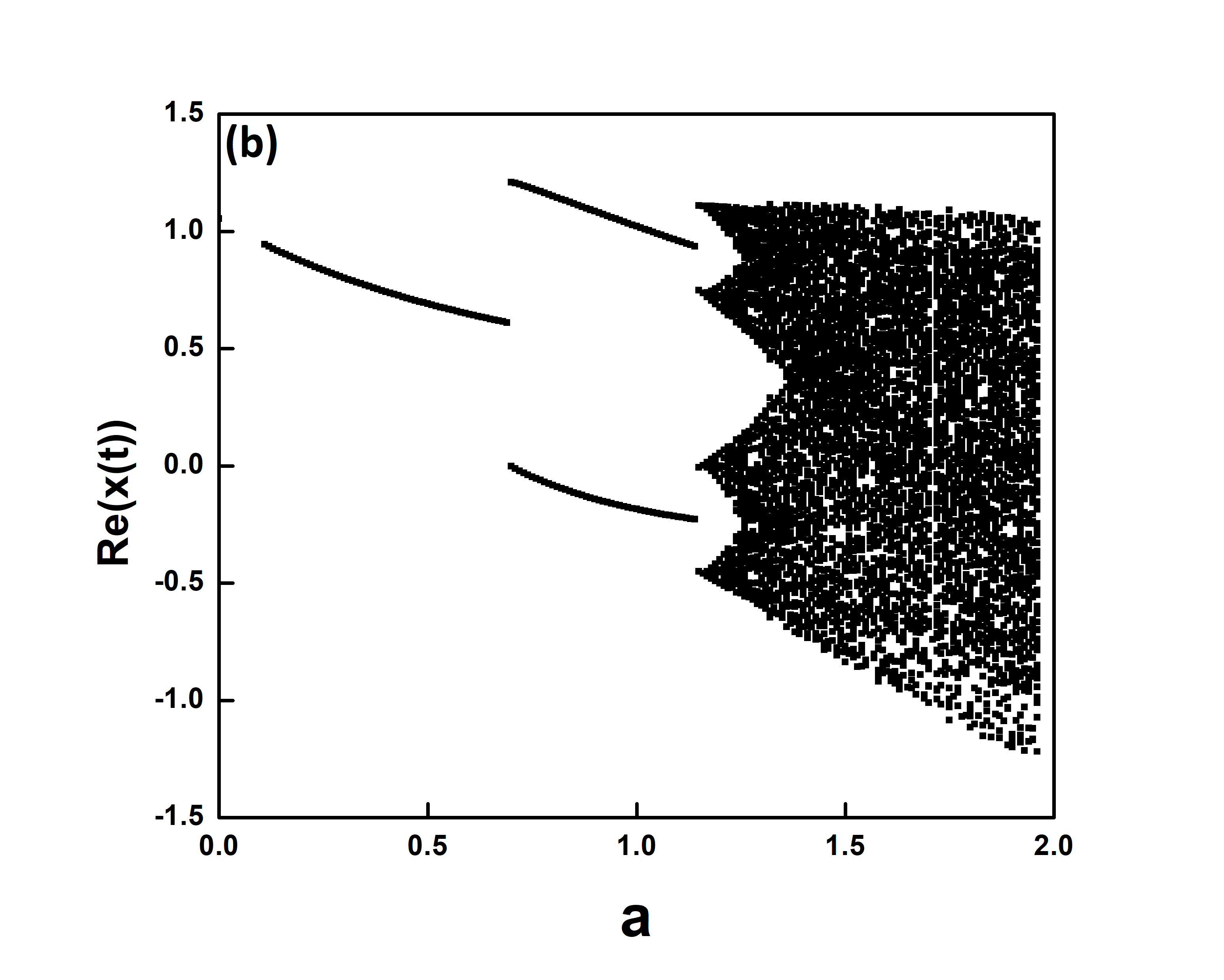
(b)

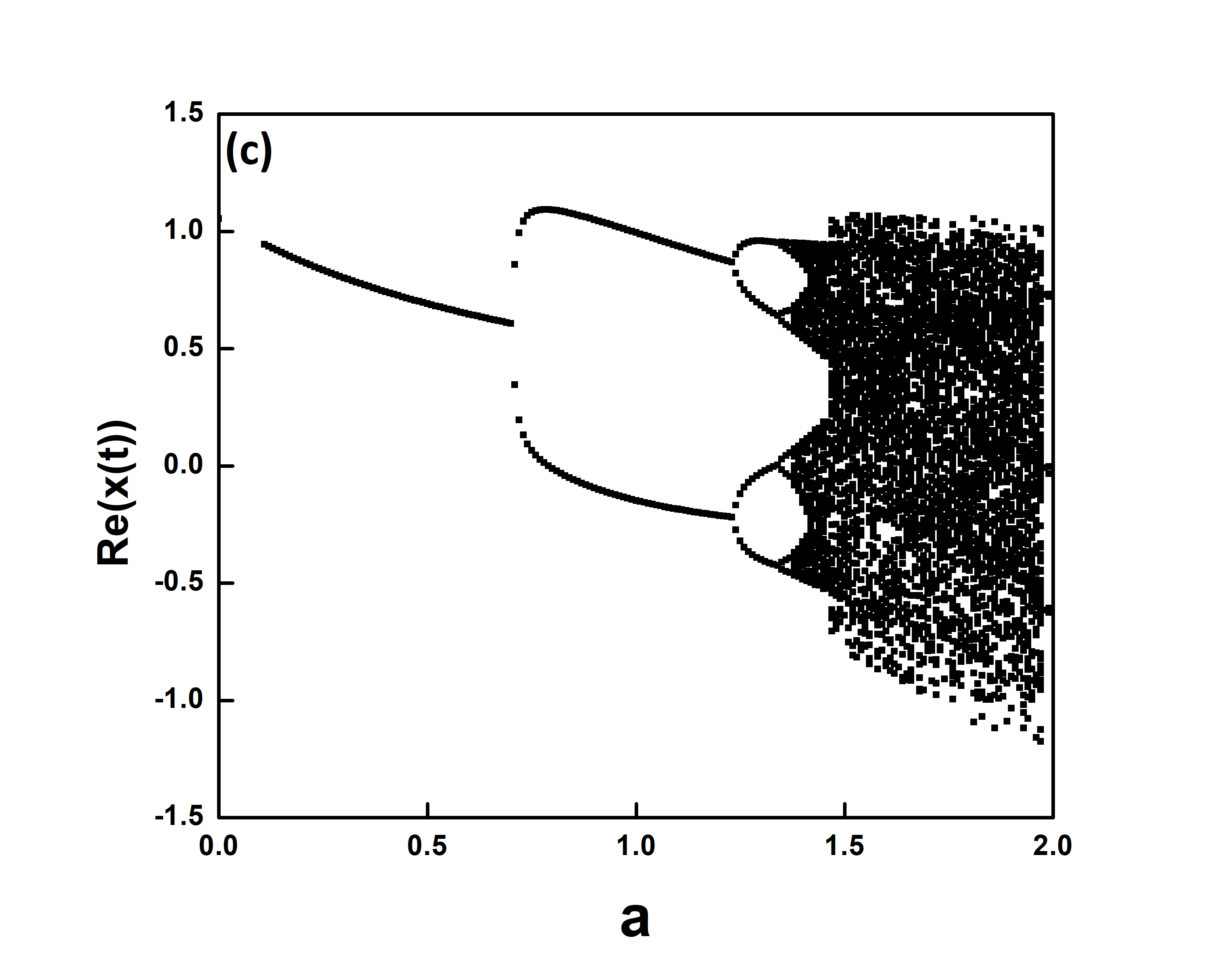
(c)

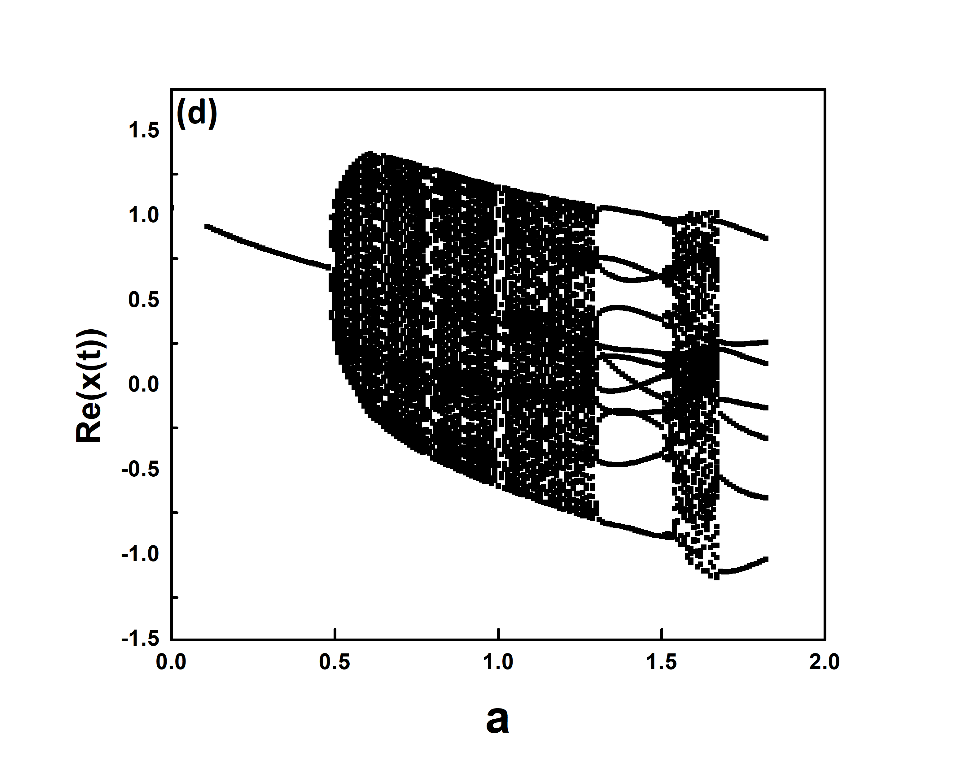
(d)

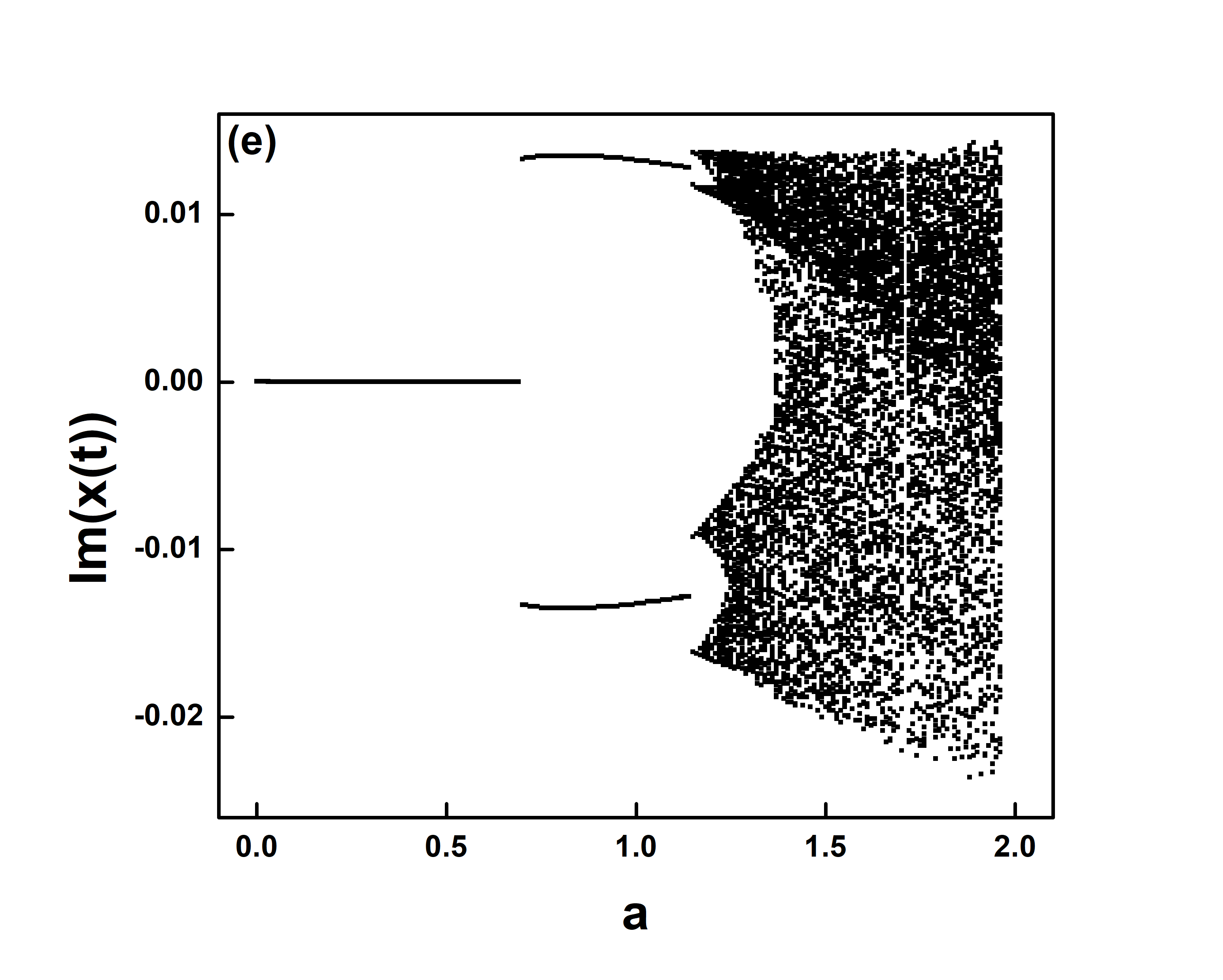
(e)

Figure 2: Bifurcation diagrams($a$ vs $Re(x(t))$) for the Lozi map (model L1) for $b=0.05$ and $\alpha_{0}=0.8$ for (a)$r=0$, (b)$r=0.01$, (c)$r=0.1$ and (d)$r=0.5$ and (e)$a$ vs $Im(x(t))$ for $\alpha_{0}=0.8,r=0.01$.

However, the situation is different for Lozi map. In this case, the chaos does not disappear. We have shown the bifurcation diagram of the Lozi map for $\alpha_{0}=0.8$ and $r=$ 0, 0.01, 0.1 and 0.5 for model L1. The span of variable values indicates that there are parameter zones that are chaotic or at least periodic with a very large period (see Figure (2)). We carry out further tests such as finding the Lyapunov exponent to confirm the presence of chaos. As mentioned above, the divergence of trajectories is exponential in our formulation and computing Lyapunov exponent is justified.

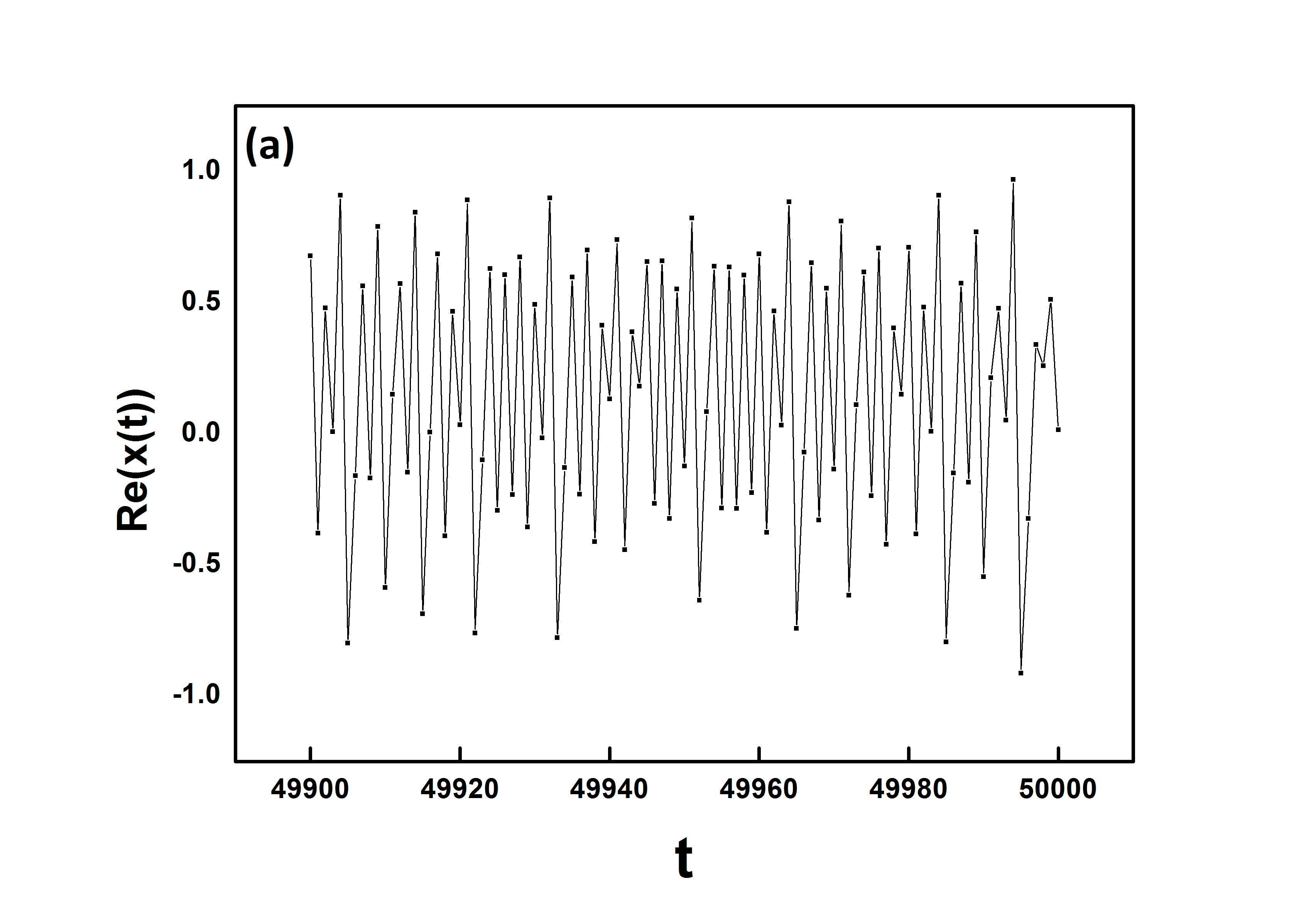
(a)

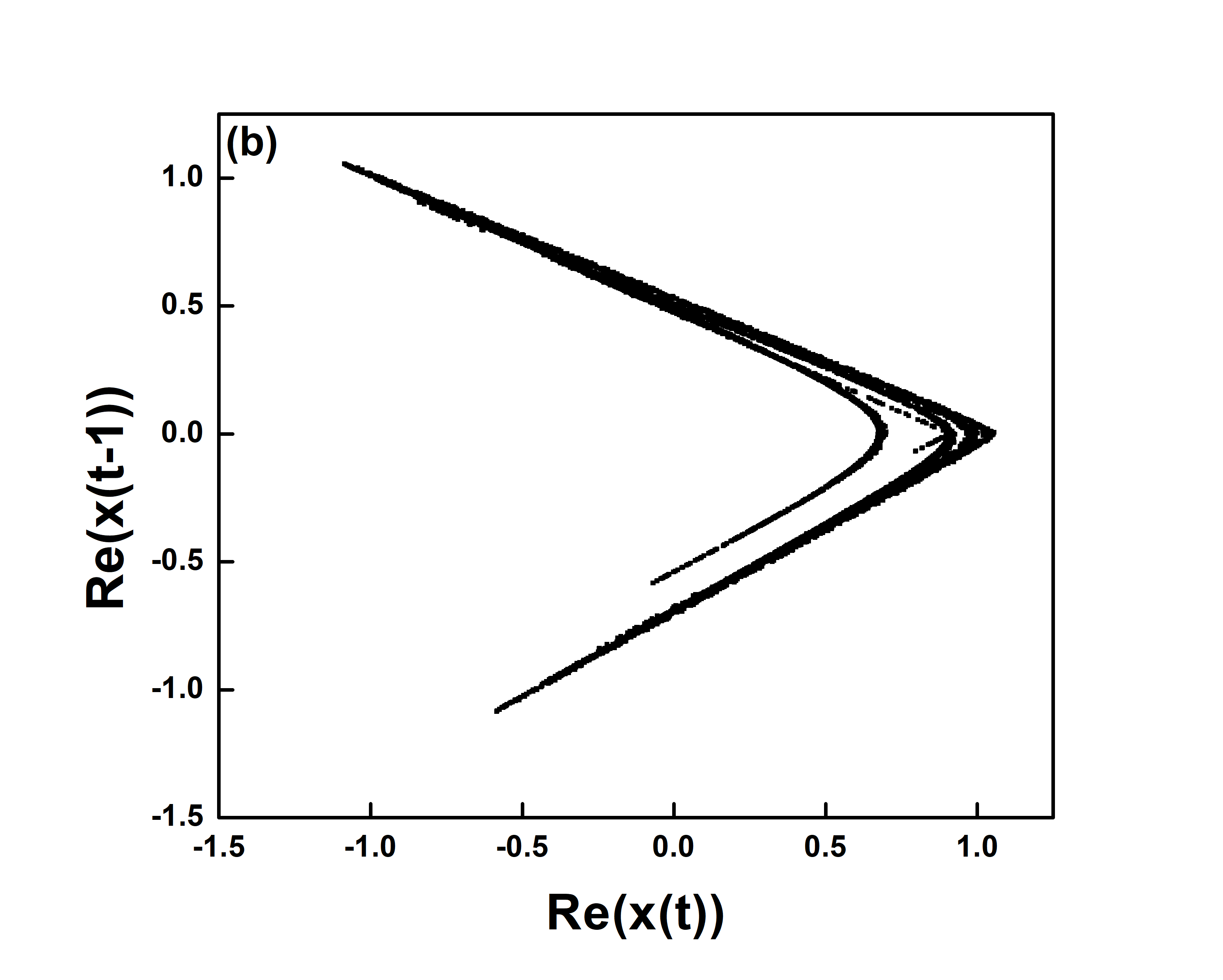
(b)

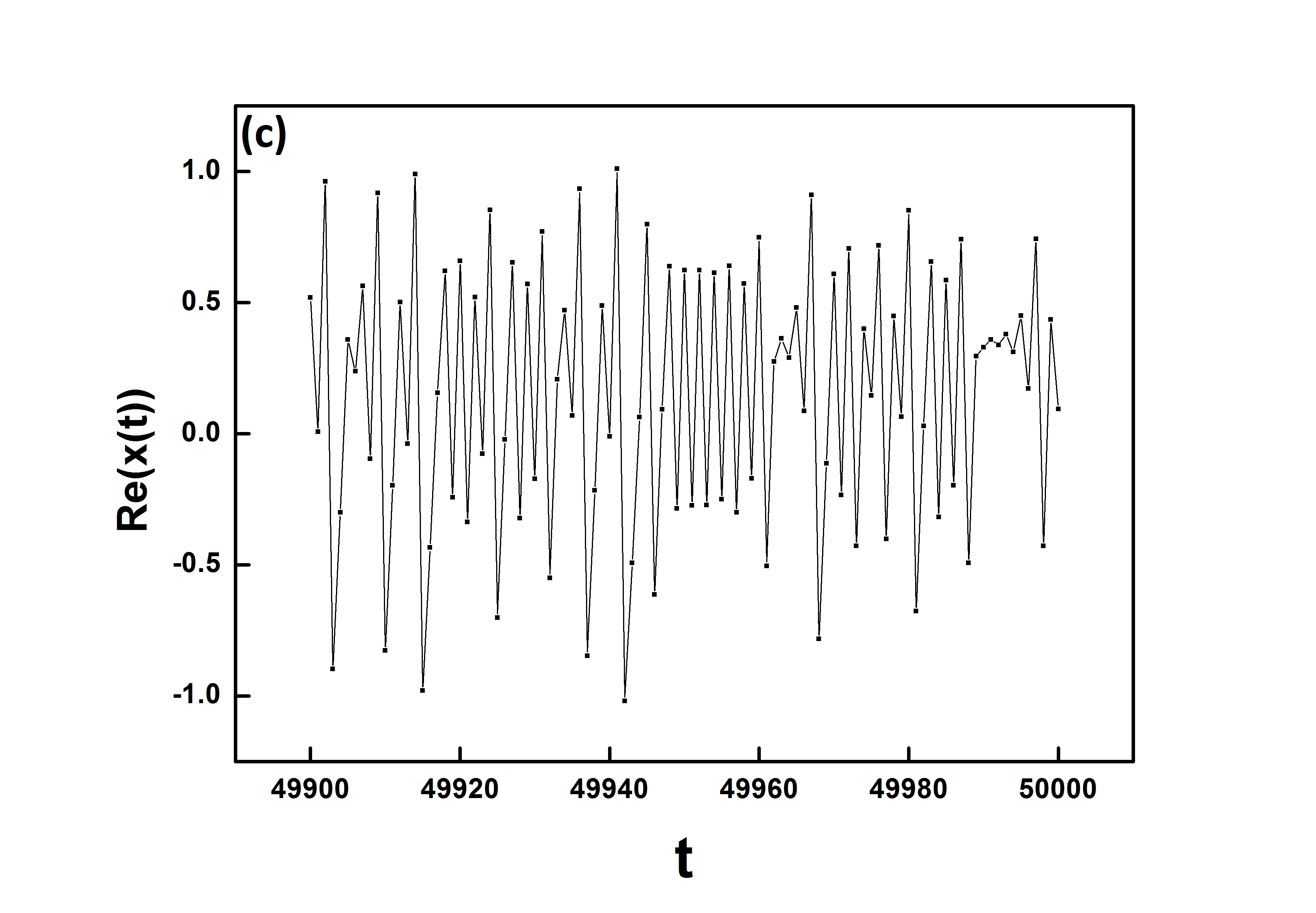
(c)

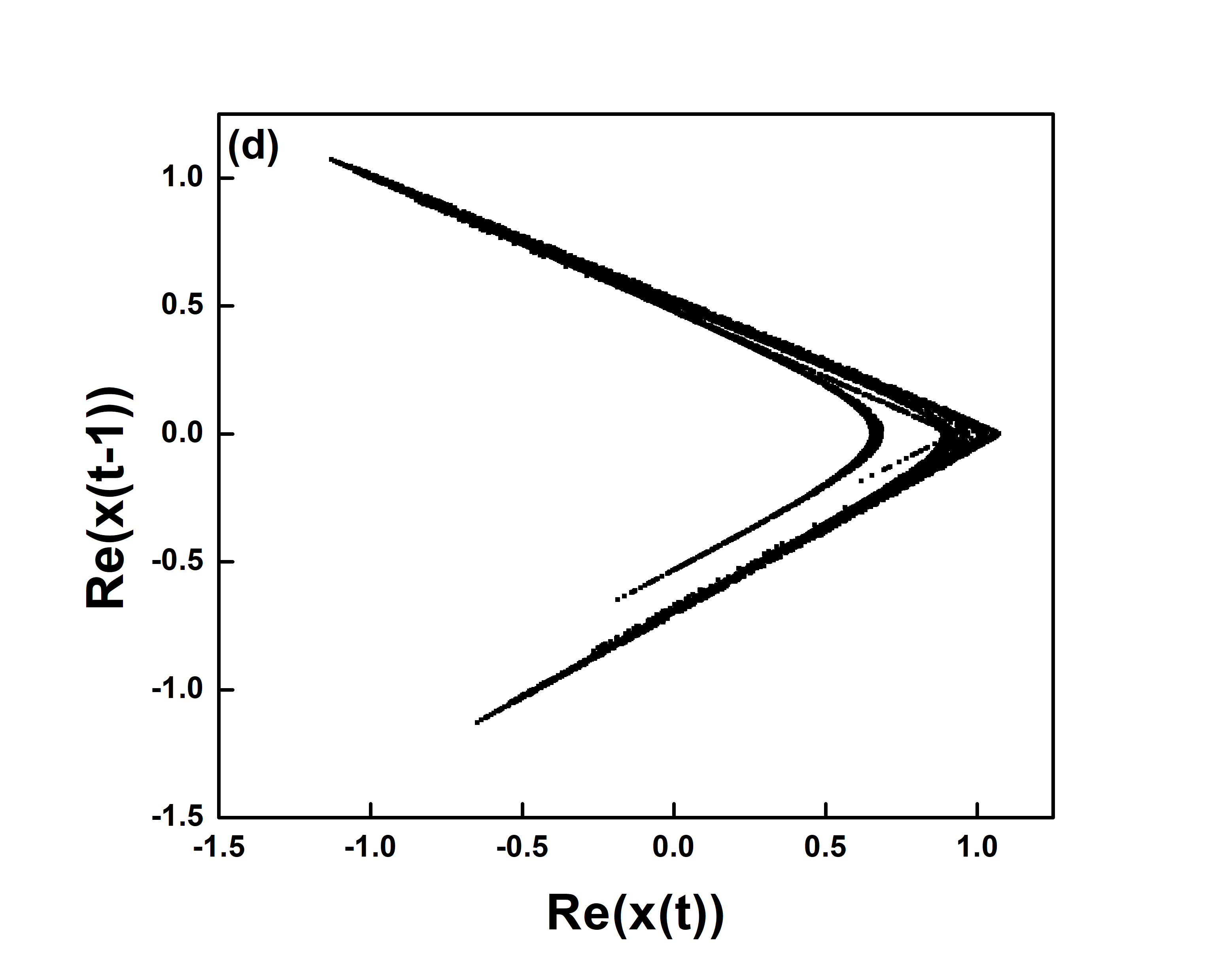
(d)

Figure 3: Attractor for Lozi map with $\alpha_{0}=0.8$, $r=0.1$, $b=0.05$ and $a=1.8$ (a) time series for corresponding to model L1 (b) attractor corresponding to a) of model L2 (c) time series corresponding to model L2 (d) attractor corresponding to c).

To check that the system is chaotic, we plot time series for $\alpha_{0}=0.8$, $r=0.1$, $a=1.8$ for both formulations. After discarding $5\times 10^{4}$ transients, we plot the attractor by plotting $x(t)$ versus $x(t-1)$ for the last $10^{4}$ time steps. We also plot the time series of the last 100 time steps. (see Figure (3)). We observe chaos in the time series, if we carry on the simulations for model L2 (eq(4)) as well as model L1 (eq(5)) of Lozi maps. To provide definitive proof that these attractors are indeed chaotic, we find Lyapunov exponents from their time series wolf1985determining ; kodba2004detecting . We use the program for finding the largest Lyapunov exponent from time series in the above works lyapmax . We find the Lyapunov exponents for both formulations of Lozi maps. For the simulation of the Lozi map, we obtain the exponent to be 0.264 for model L1 and exponent 0.326 for model L2 for the parameters mentioned in the caption. Since both the systems show positive values of the Lyapunov exponent, it confirms our prognosis that the Lozi map shows chaos for the difference equation of complex fractional order.

Hénon map is an analytic function and the bifurcation diagram (1) does not show chaos for complex fractional-order. (The bifurcation diagram is concerning model H1. However, a similar diagram is obtained for model H2.) The chaotic attractors vanish with the slightest introduction of an imaginary part in the order. There could be a link between the absence of chaos for complex fractional ordered maps and the analytic nature of the function maps. To investigate if it is indeed so, we analyze two more smooth functions i.e., continuous and differentiable maps. We consider two of the most popular maps, Gauss and logistic maps. Figure (4) shows the bifurcation diagram for Gauss and logistic maps. We observe that the chaos vanishes as the order gets slightly complex as in the case of the Hénon map.

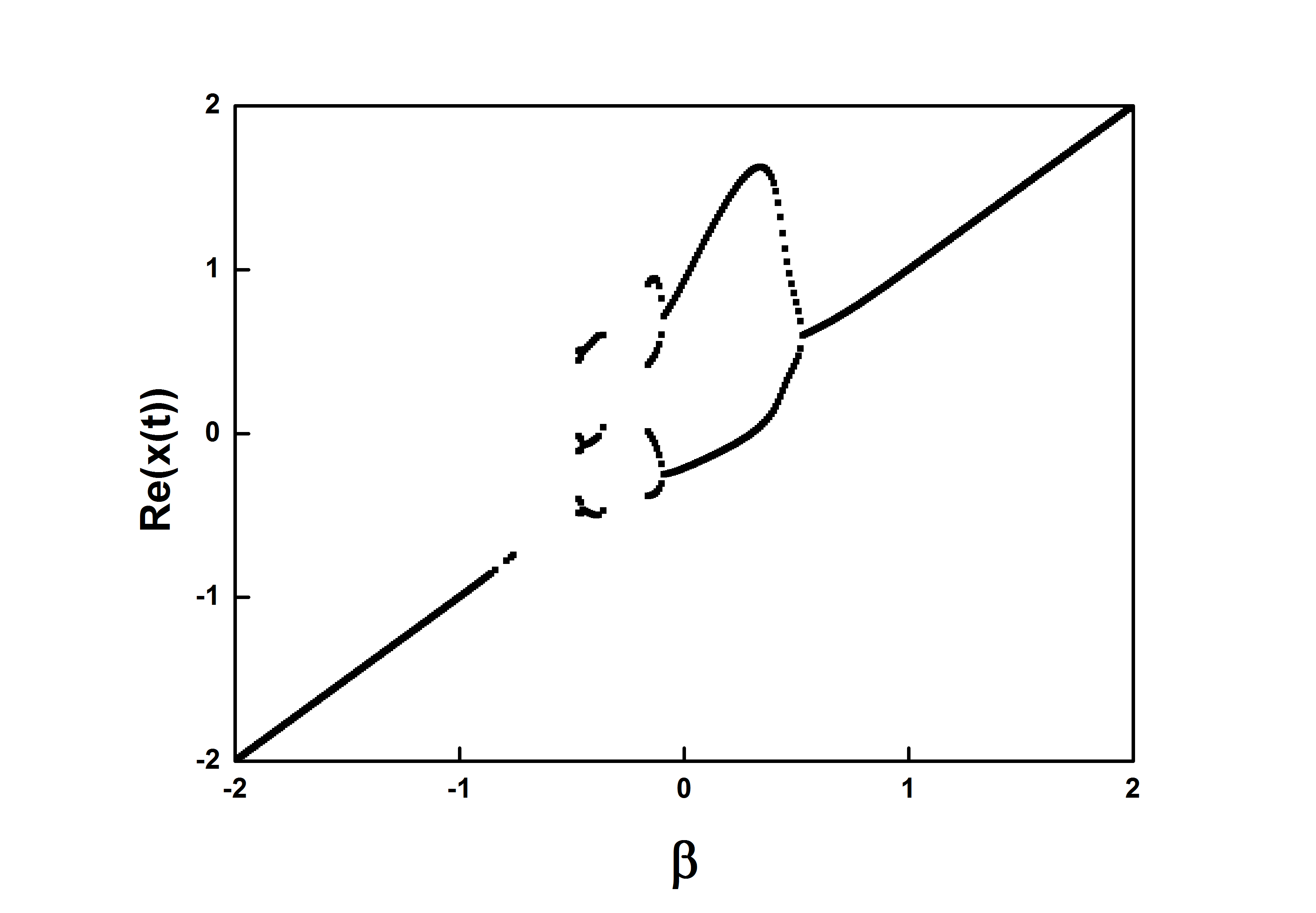
(a) Gauss map with $\alpha_{0}=0.7$ and $r=0.01$.

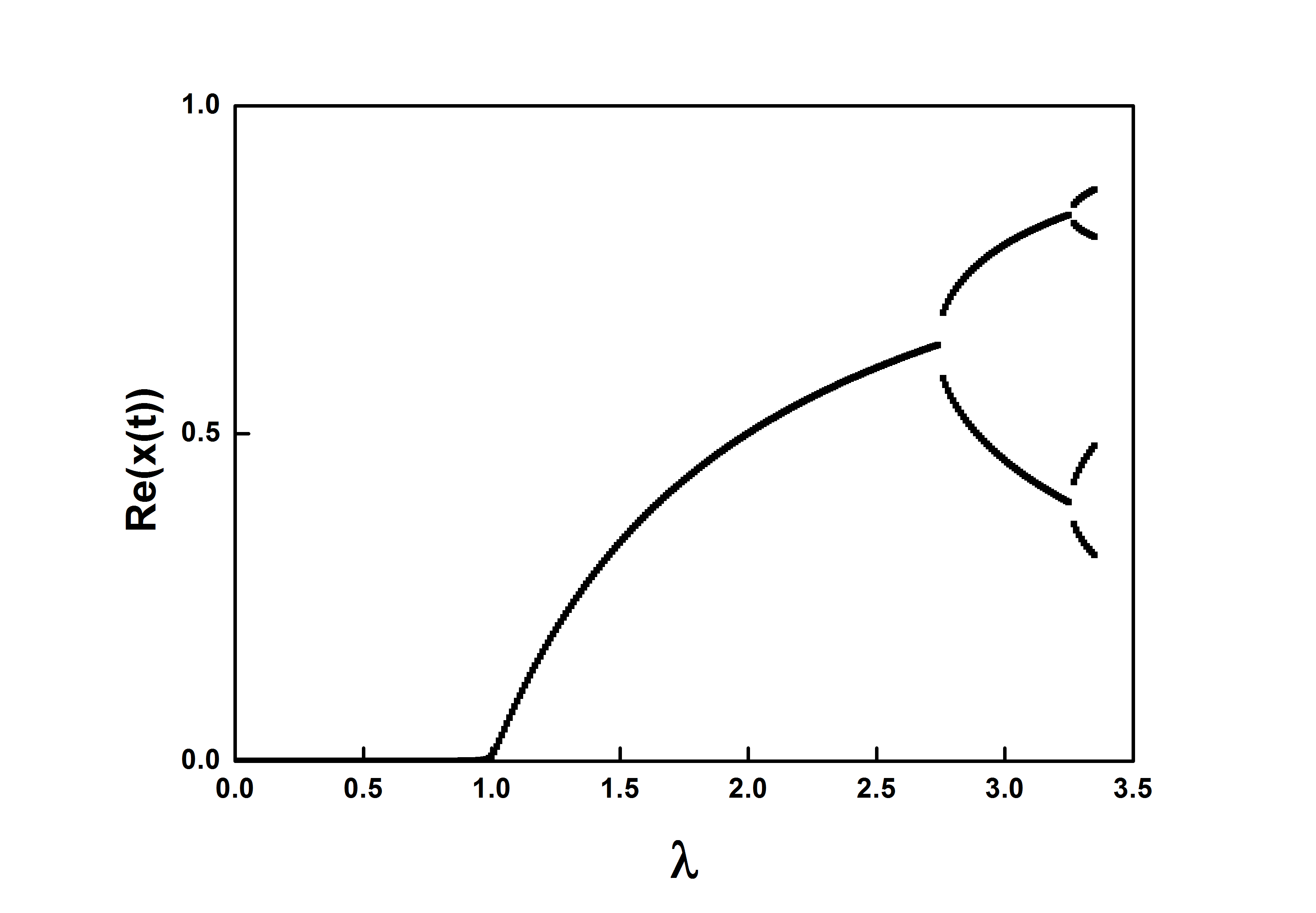
(b) Logistic map with $\alpha_{0}=0.8$ and $r=0.01$.

Figure 4: Bifurcation diagrams for Gauss map and logistic map. The bifurcation diagram was observed for the system by taking $10^{4}$ timesteps and the last 120 values have been plotted. No chaos was observed for these maps.

If the chaotic attractor is ergodic, different initial conditions lead to the same attractor. In general, in integer-order $1d$ maps, we do not observe multistability and different initial conditions lead to the same attractor. But for maps of complex fractional-order showing chaos, we observe multistability. This effect may be due to extending the order of difference equations and making $\alpha$ complex. It also could be an artifact of the fact that the variables like $x(t)$ or $y(t)$ become complex even if we start with real initial conditions. To understand this effect, we carry out simulations for real fractional order maps by giving complex initial conditions. We study the effect of complex initial conditions for maps of fractional real order. For Gauss, logistic, and Hénon maps, we plot the bifurcation diagram for real and complex initial conditions (see Figure (6)). For the logistic map, we observe fixed point, period-2 and period-4 orbits. Period-2 orbits can be found analytically for the logistic map and the method is outlined in the appendix. We observe no multistability in this case. We show basin of attraction for period-4 points of logistic map for $\lambda=3.29,\alpha_{0}=0.8,r=0.01$ in figure(5). We note that all initial conditions which do not converge to period-4 escape to infinity. The basin has an interesting fractal structure and can be viewed as Julia set for this system. Thus, there is no multistability in this system. Furthermore, we do not observe any aperiodic attractor. We spot a correlation between the existence of chaos and the initial conditions. It is a crucial revelation that chaos vanishes in all three continuous and differentiable maps (Gauss, logistic, and Hénon maps) when the initial conditions are complex for real fractional order i.e., for $r=0,0<\alpha_{0}<1$. In prior studies of fractional real order maps, initial conditions were real constants as seen in deshpande2016chaos .

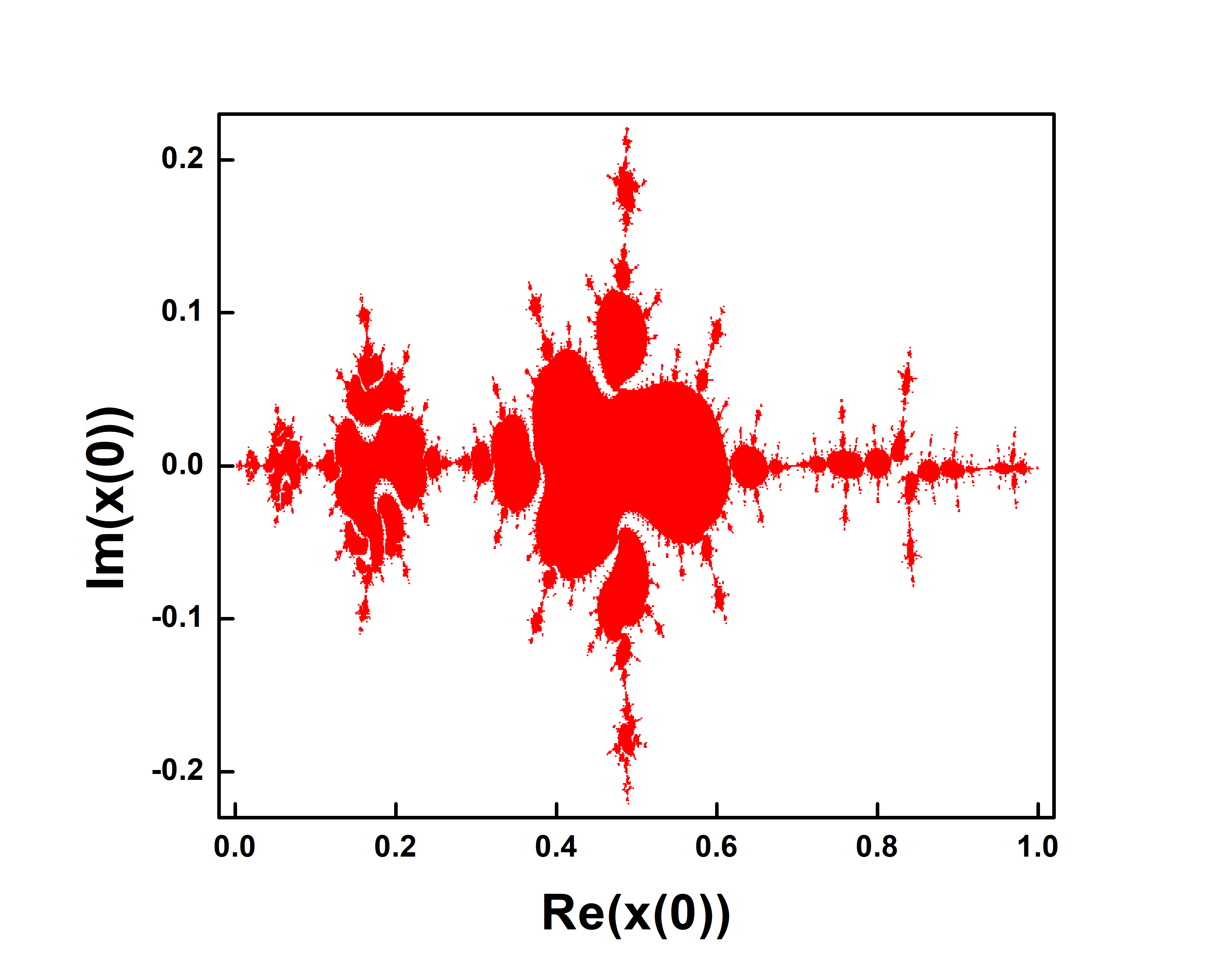
Figure 5: Basin of logistic map with $\alpha_{0}=0.8$ and $r=0.01$.

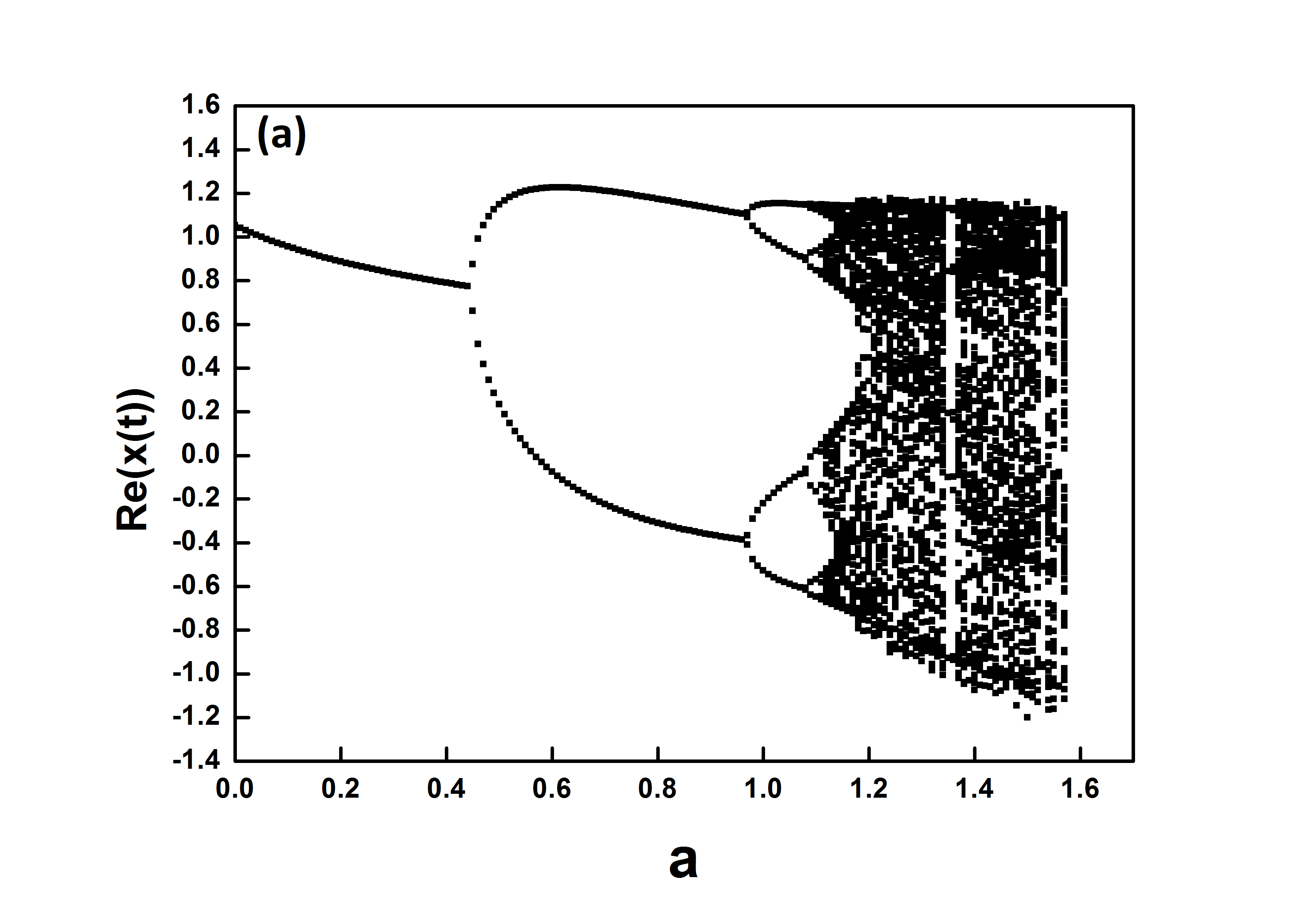
(a) Hénon map with $\alpha_{0}=0.8$, $r=0$, $x_{0}=(0.2,0)$ and $x_{(-1)}=(0.1,0)$.

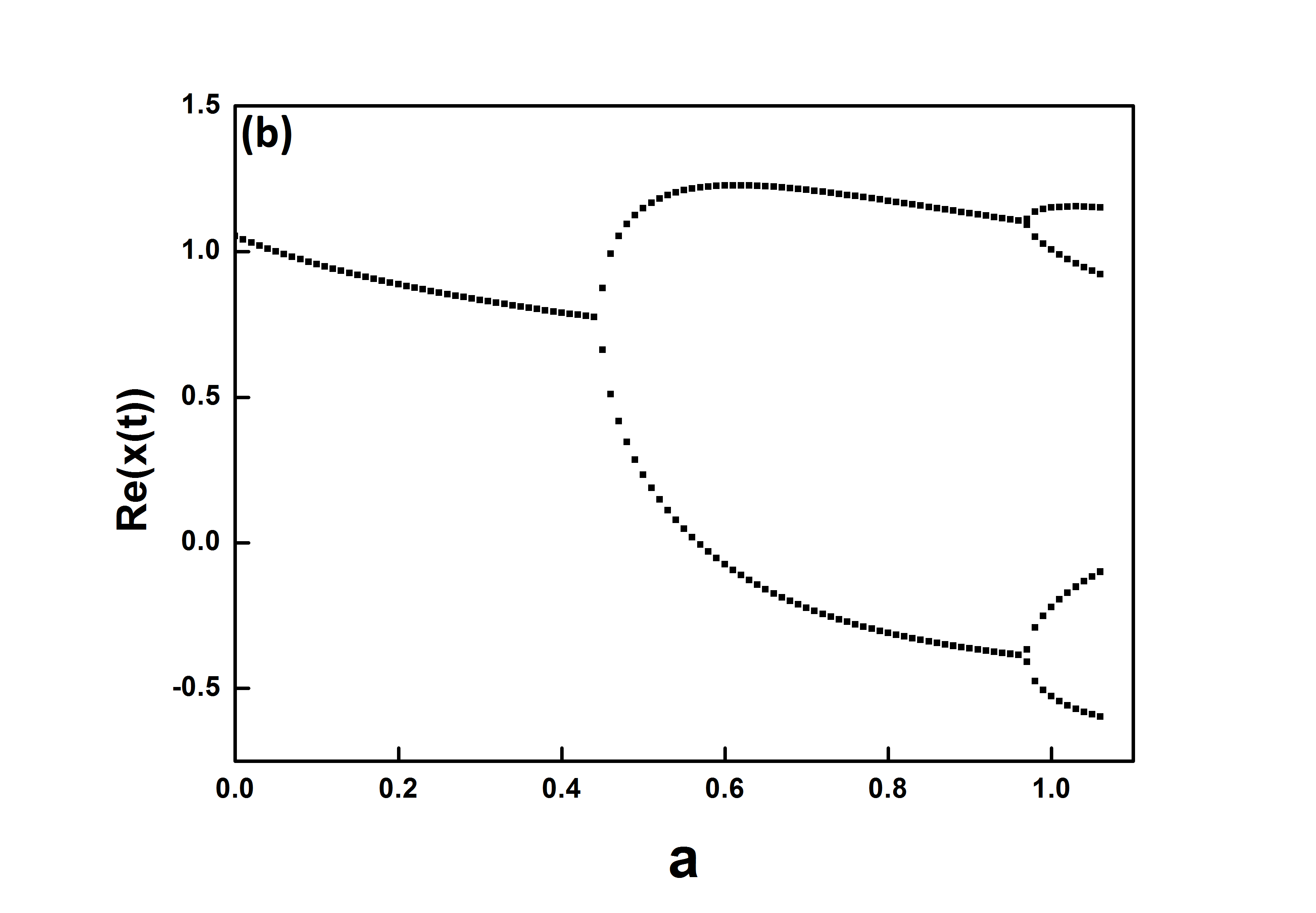
(b) Hénon map with $\alpha_{0}=0.8$, $r=0$, $x_{0}=(0.2,0.1)$ and $x_{(-1)}=(0.1,0.1)$.

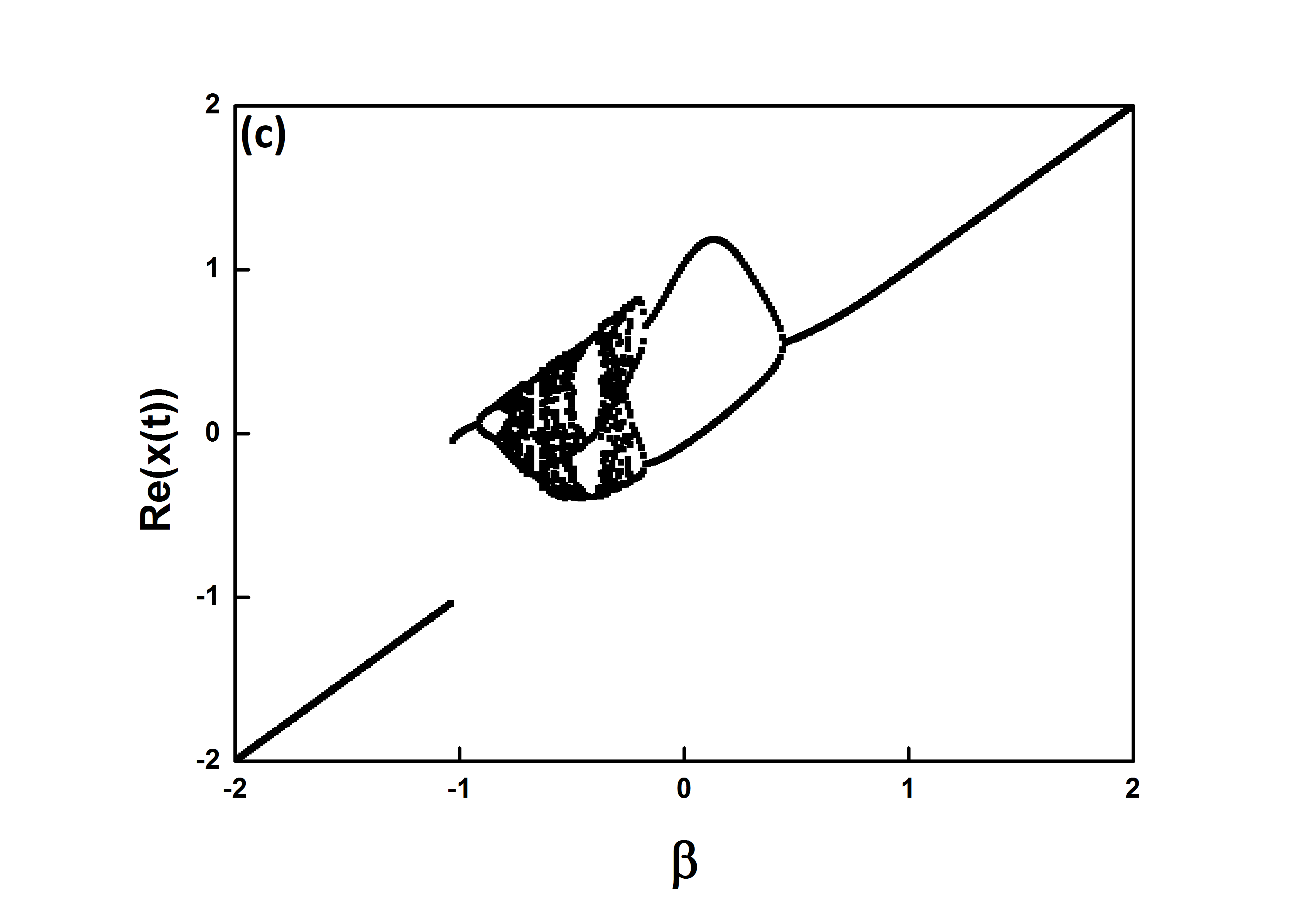
(c) Gauss map with $\alpha_{0}=0.9$, $r=0$ and $x_{0}=(0.1,0)$.

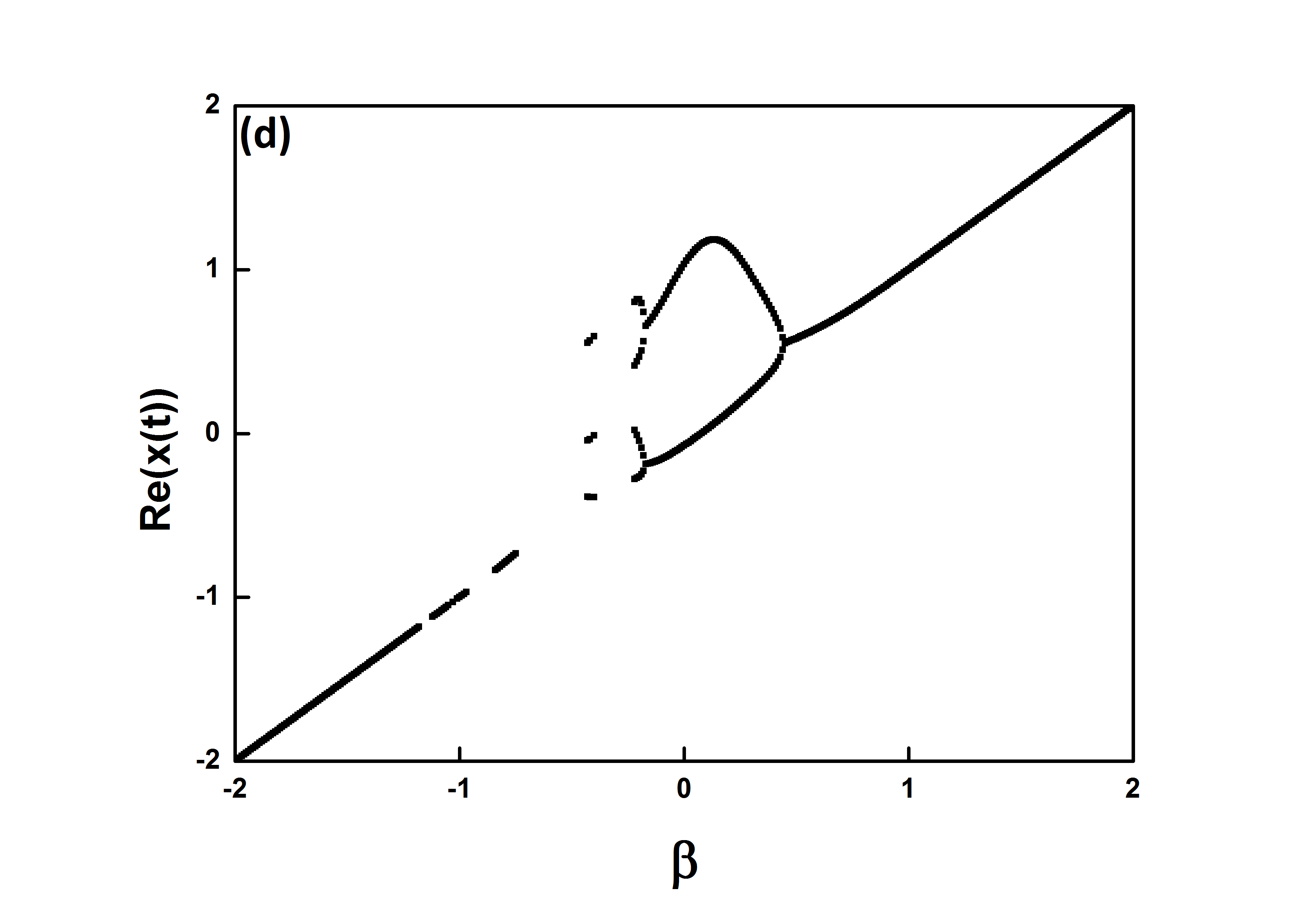
(d) Gauss map with $\alpha_{0}=0.9$, $r=0$ and $x_{0}=(0.1,0.1)$.

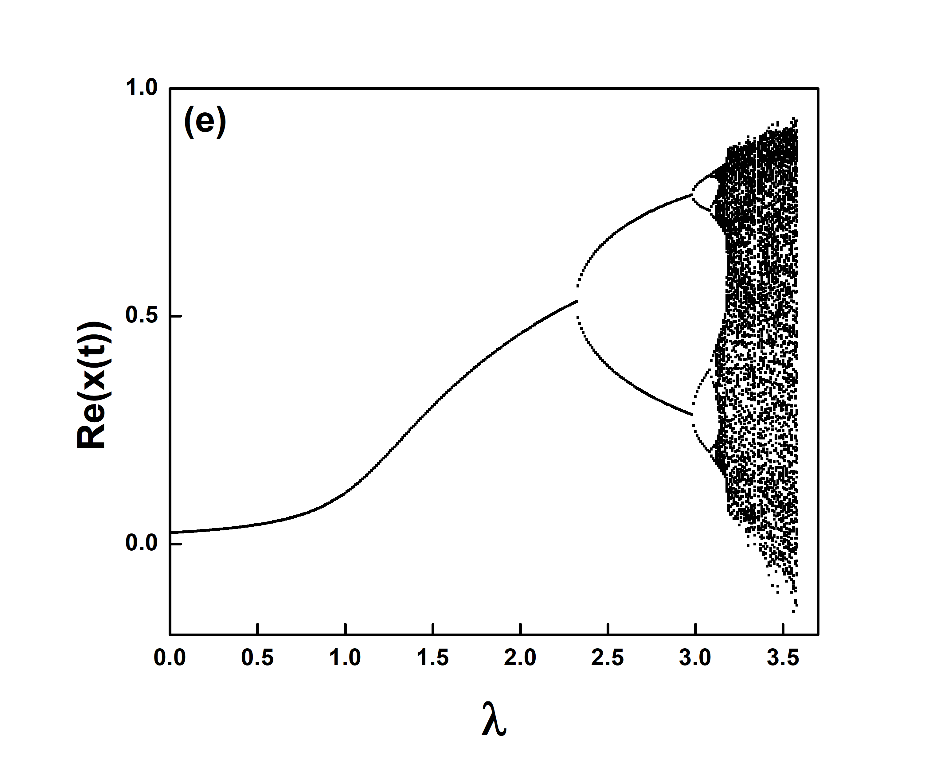
(e) Logistic map with $\alpha_{0}=0.2$, $r=0$ and $x_{0}=(0.2,0)$.

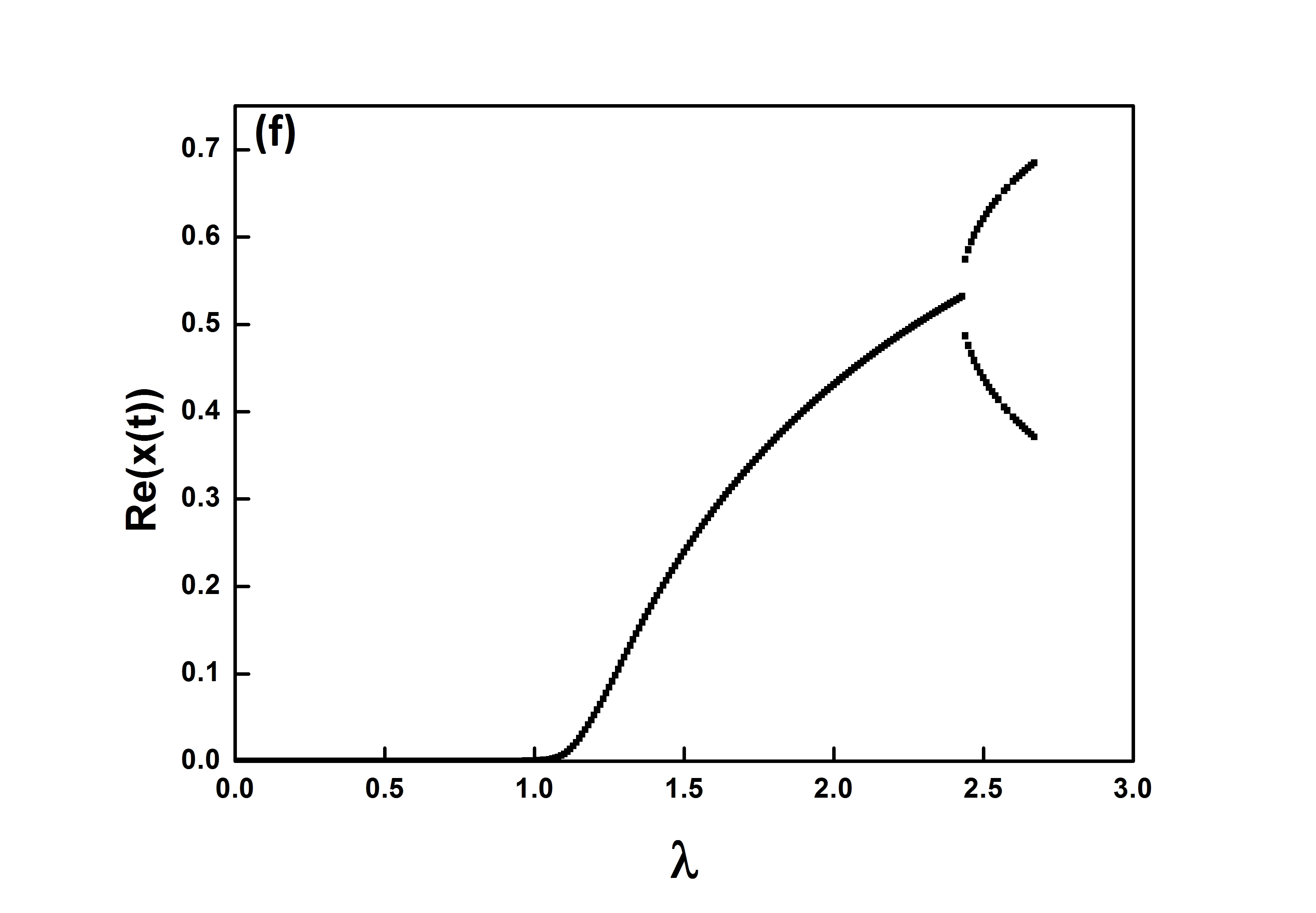
(f) Logistic map with $\alpha_{0}=0.2$, $r=0$ and $x_{0}=(0,0.01)$.

Figure 6: Loss of chaos for complex initial conditions in Hénon, Gauss, and logistic map for real fractional order (b,d,f). The bifurcation diagrams for real initial conditions are also shown for comparison (a,c,e).

We study discontinuous maps such as the Bernoulli map and the circle map, as well as continuous but non-differentiable, such as the tent map. The bifurcation diagram (see Figure (7)) shows that, even with the introduction of complex fractional-order, the chaotic attractor is not destroyed. Thus, we may correlate the existence of chaos for complex fractional-order with the analytic nature of the maps. In discontinuous maps, we find chaotic attractors in all cases namely, a) Real fractional-order and real initial conditions b) Real fractional-order and complex initial conditions c) Complex fractional order and real initial conditions and d) Complex fractional order and complex initial conditions. On the other hand, for Hénon, logistic, and Gauss maps, we observe chaotic attractor only for real fractional-order and real initial conditions.

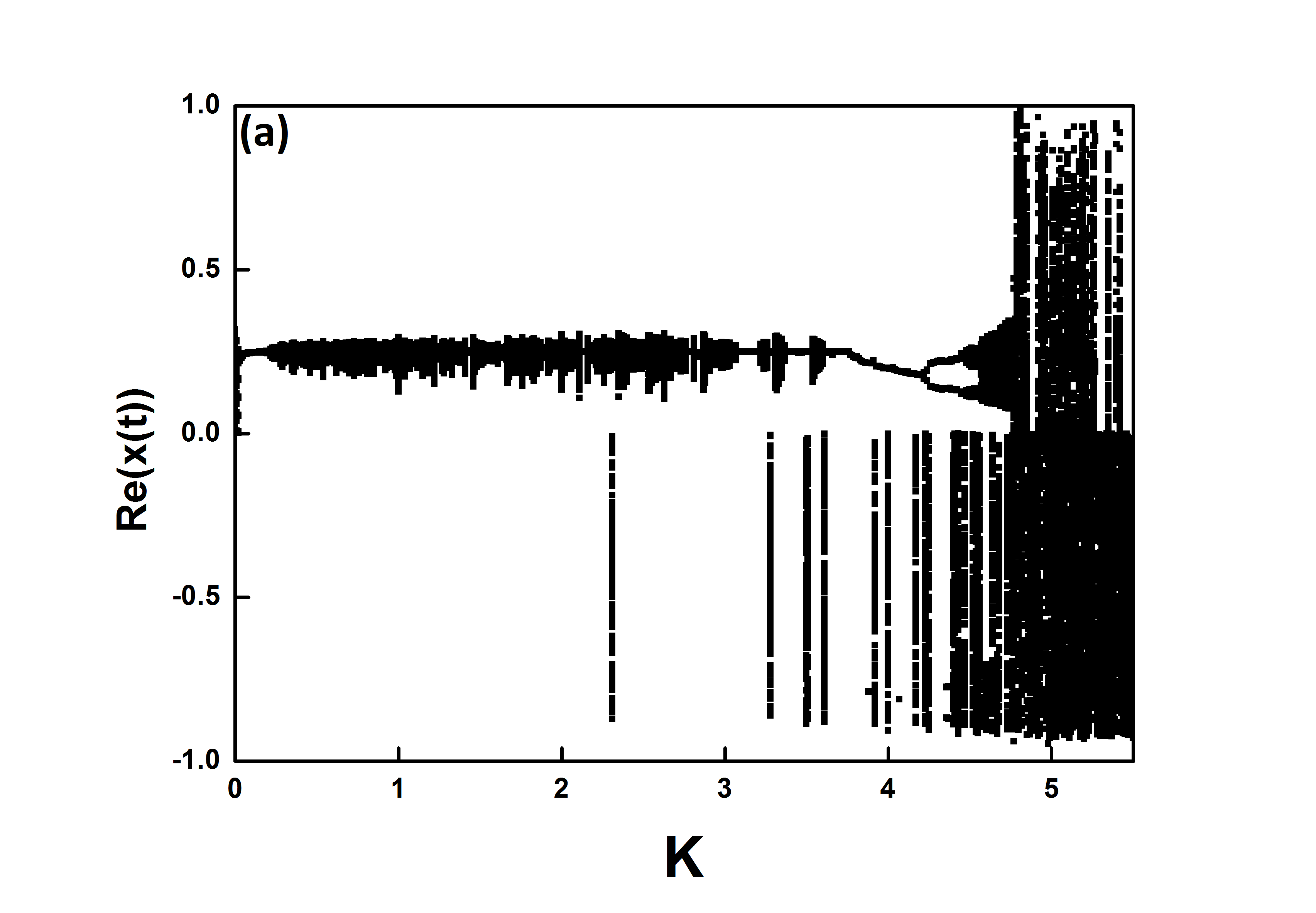
(a) Circle map with $\alpha_{0}=0.9$, $r=0.1$ and $x(0)=0$.

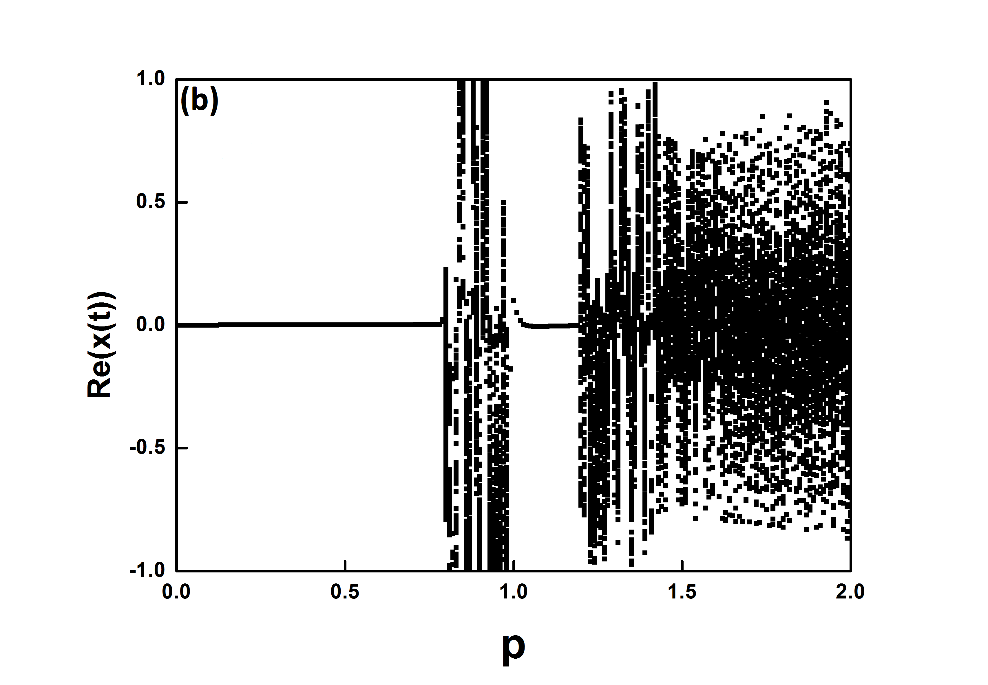
(b) Bernoulli map with $\alpha_{0}=0.7$, $r=0.5$ and $x(0)=0$.

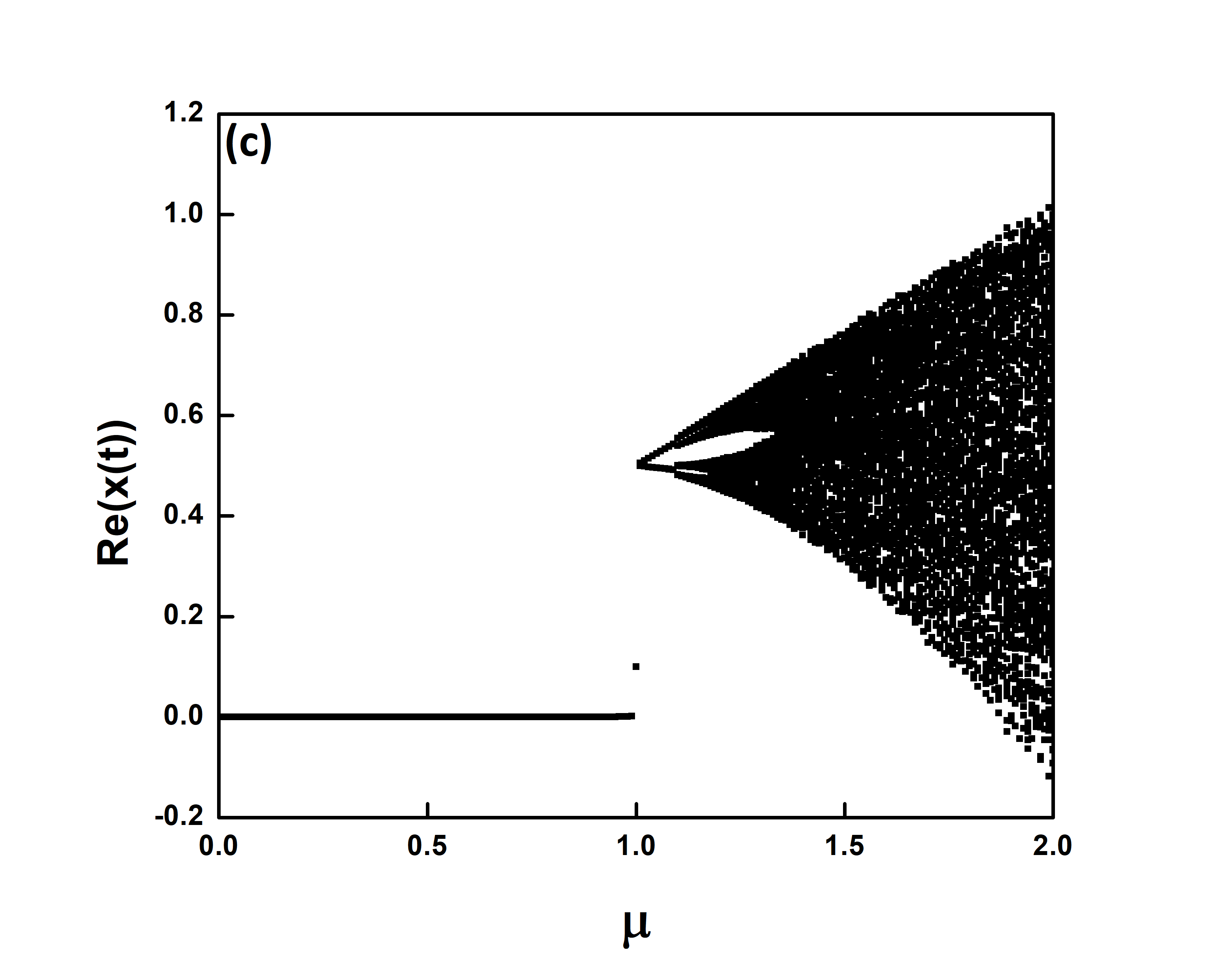
(c) Tent map with $\alpha_{0}=0.8$, $r=0.01$ and $x(0)=0$.

Figure 7: Bifurcation diagrams for circle map, Bernoulli map, and tent map.

We note that extremely strange bifurcations are observed in the Lozi map (model L1) of complex fractional-order. We have shown bifurcation diagrams for $\alpha=0.4+0.3\iota$ and $\alpha=0.4+0.5\iota$ in Figures (9a and 9b) which clearly shows the possibility of very large periods and the rich bifurcation structure which is usually not seen in integer-order systems. From these figures, it is clear that two different initial conditions lead to different bifurcation diagrams for the Lozi map which is a clear indication of multistability.

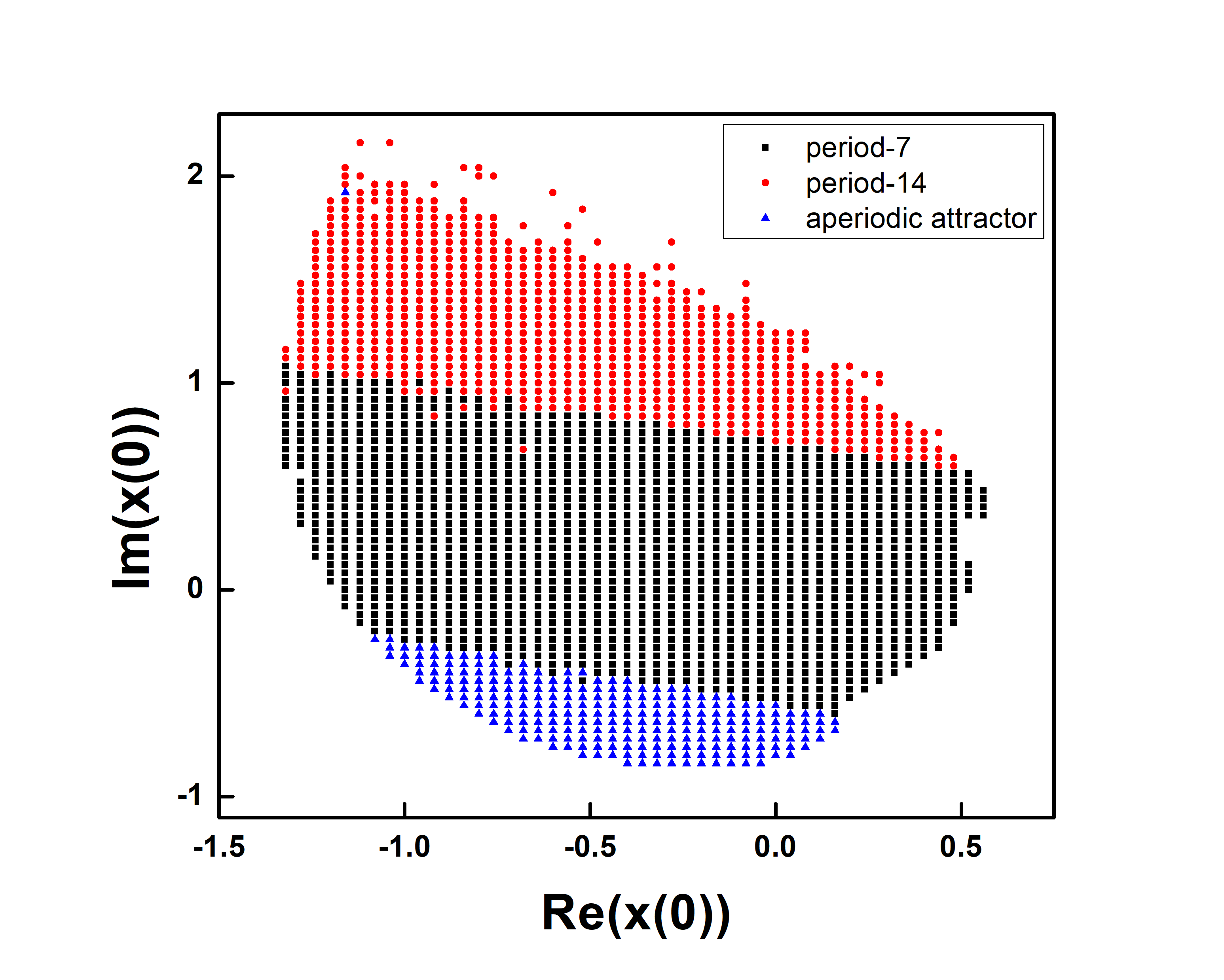
(a) Basin of attraction for Lozi map.

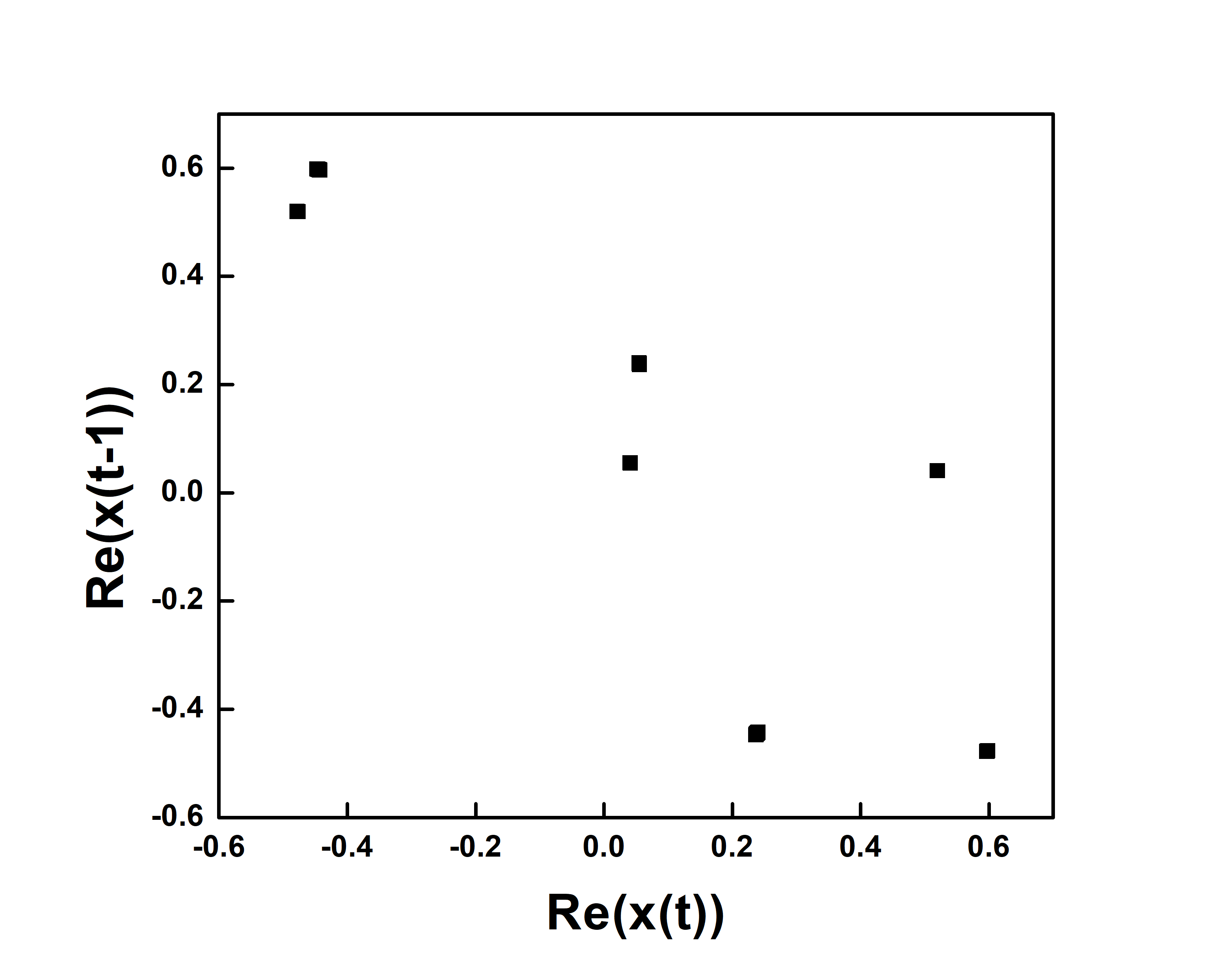
(b) Attractor of period-7 with $x(0)=-0.5+1.2\iota$.

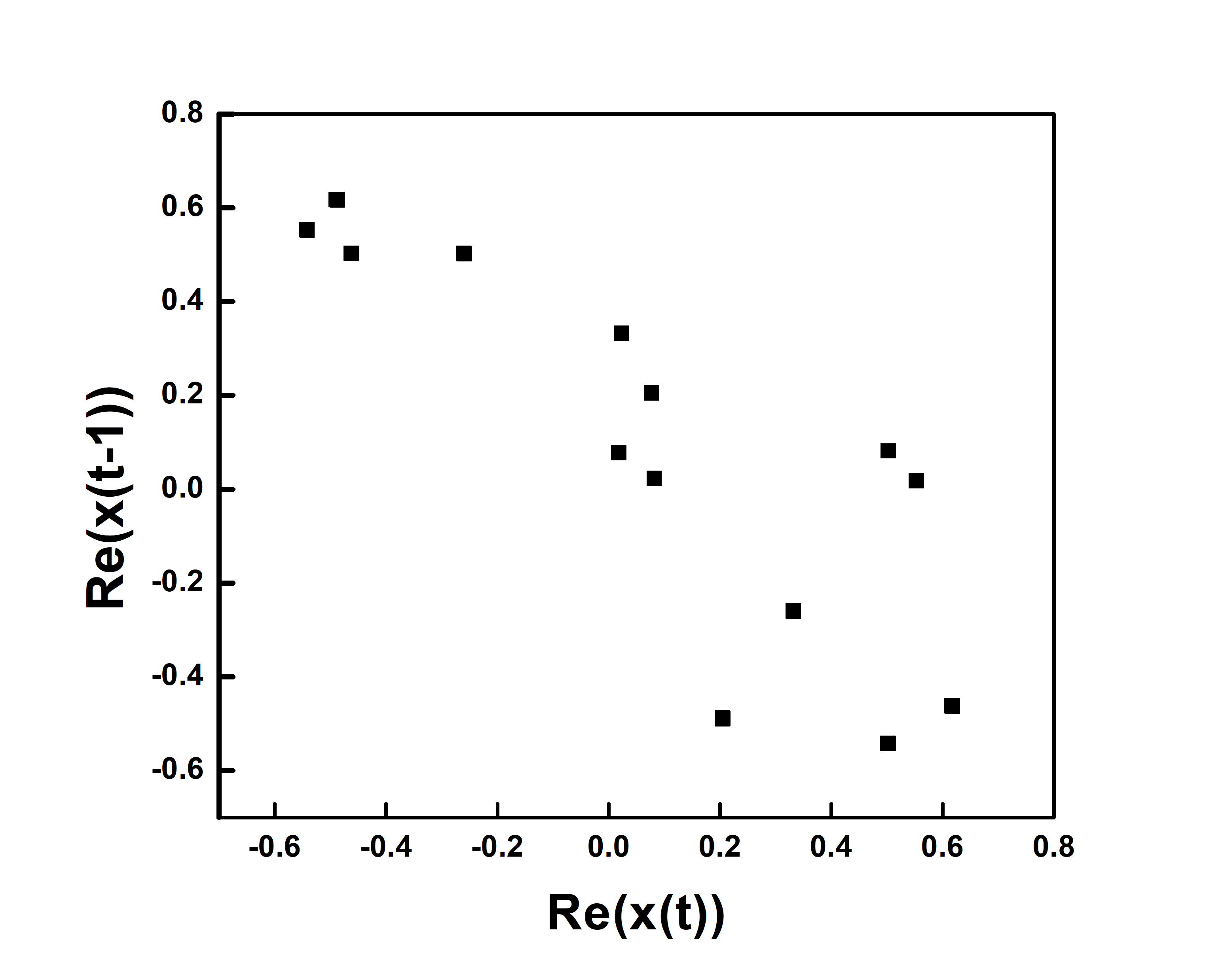
(c) Attractor of period-14 with $x(0)=-0.8-0.5\iota$.

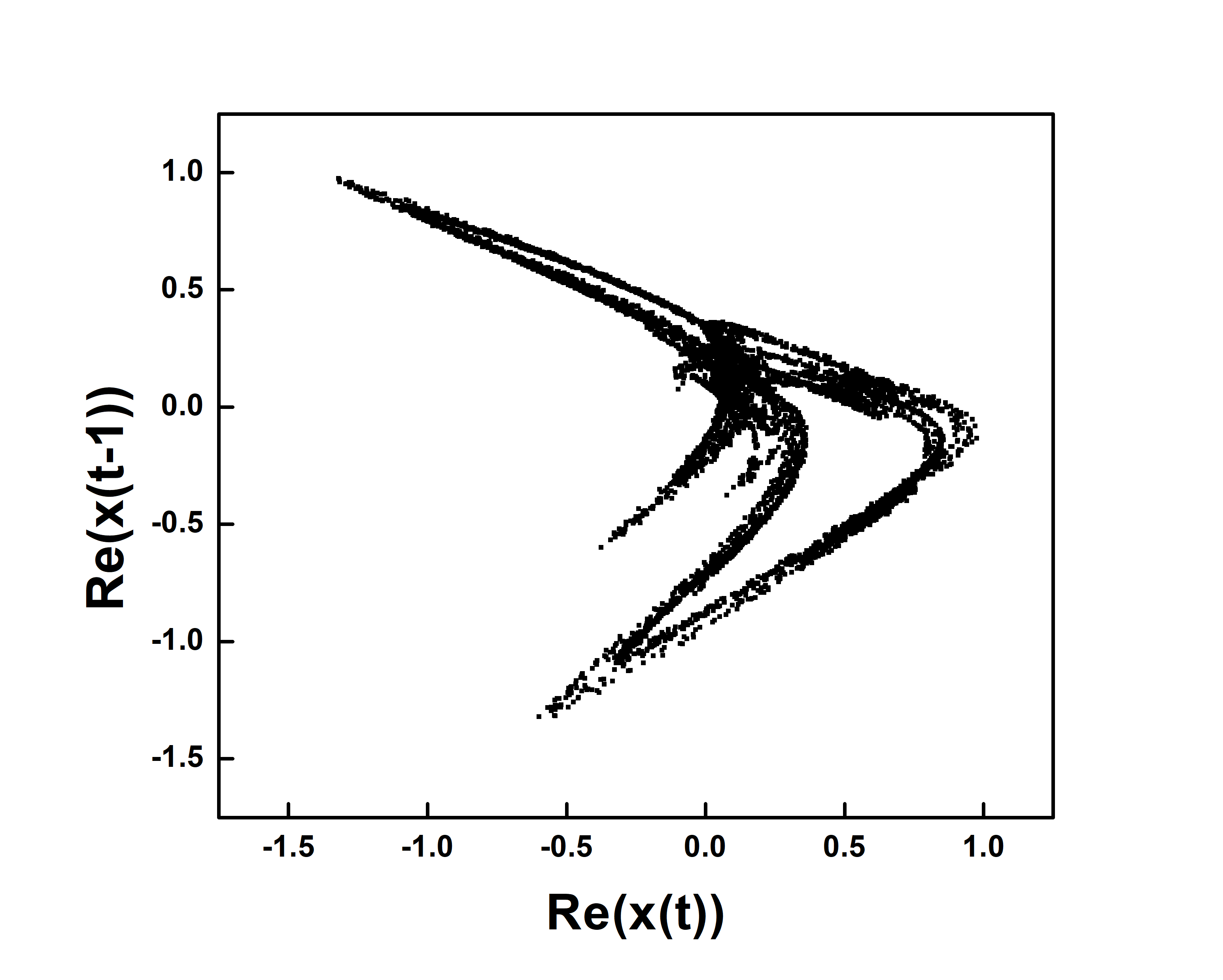
(d) Aperiodic attractor with $x(0)=0.3+0.4\iota$.

Figure 8: Lozi map showing multiple attractors for varying combinations of initial conditions.

For Lozi map, for $x(-1)=0.4+\iota$, $\alpha_{0}=0.4+0.5\iota,a=1.8,b=0.05$ three different attractors are realized for different initial values of $x(0)$. We observe period-7, period-14, and aperiodic attractor. These basins and attractors are shown in figure(8).

We have also shown the bifurcation diagram with two different initial conditions for Bernoulli, circle, and tent map in Figures (9c, 9d, and 9e). It is clear that the bifurcation diagram changes. Thus, different attractors are reached with different initial conditions. Thus, these maps clearly show multistability. We studied basins of attraction of different attractors in circle map. For $a=4.4$, we observe both period-2 and aperiodic attractor. However, basins of attractors are intermingled and initial conditions leading to periodic attractor are randomly distributed and do not have a smooth or fractal structure.

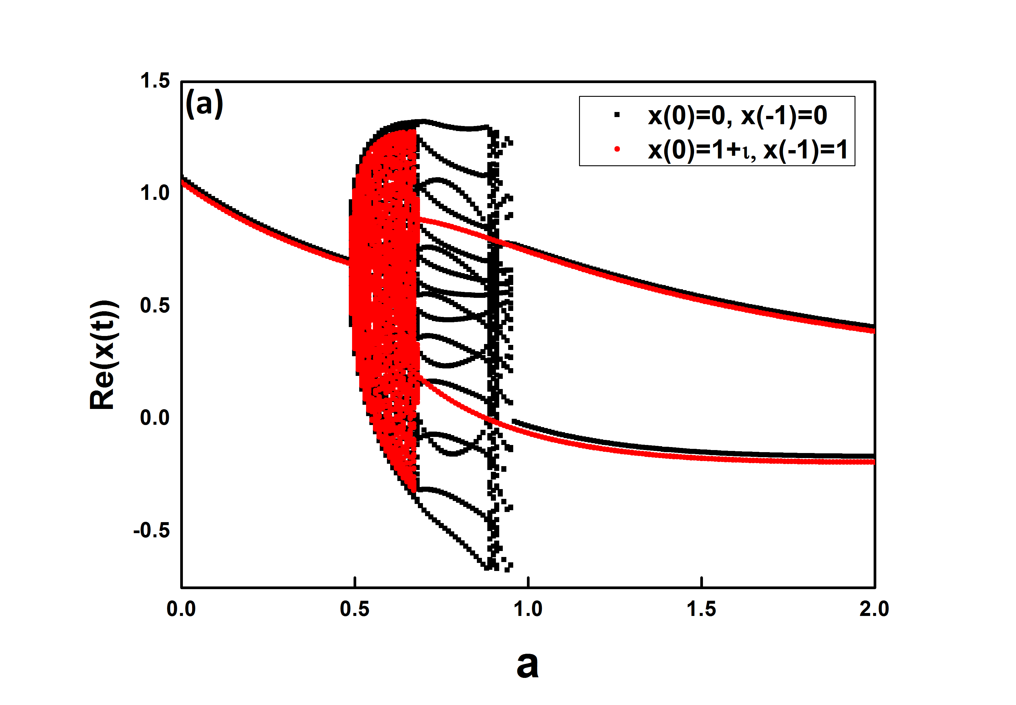
(a) Lozi map with $\alpha=0.4+0.3\iota$.

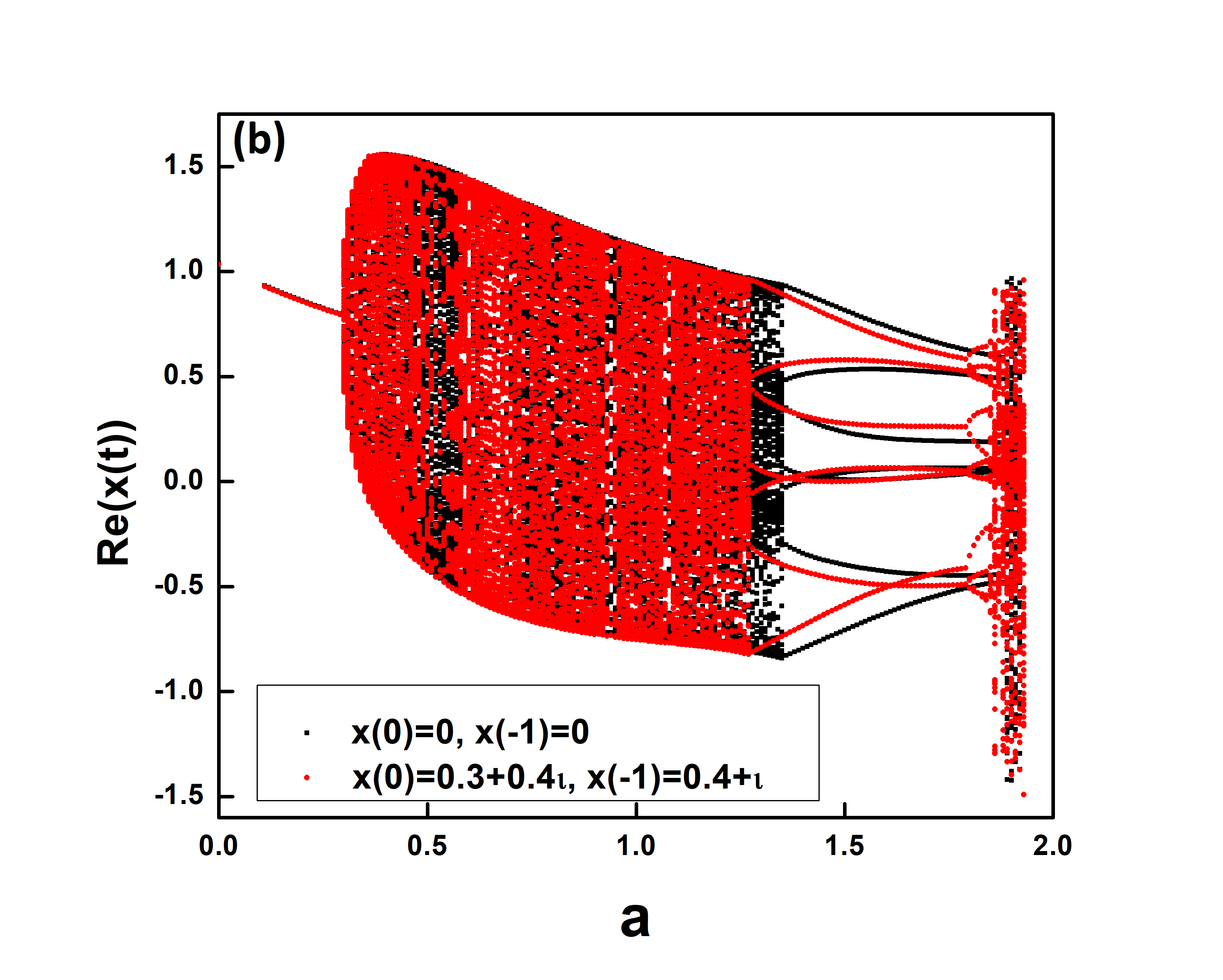
(b) Lozi map with $\alpha=0.4+0.5\iota$.

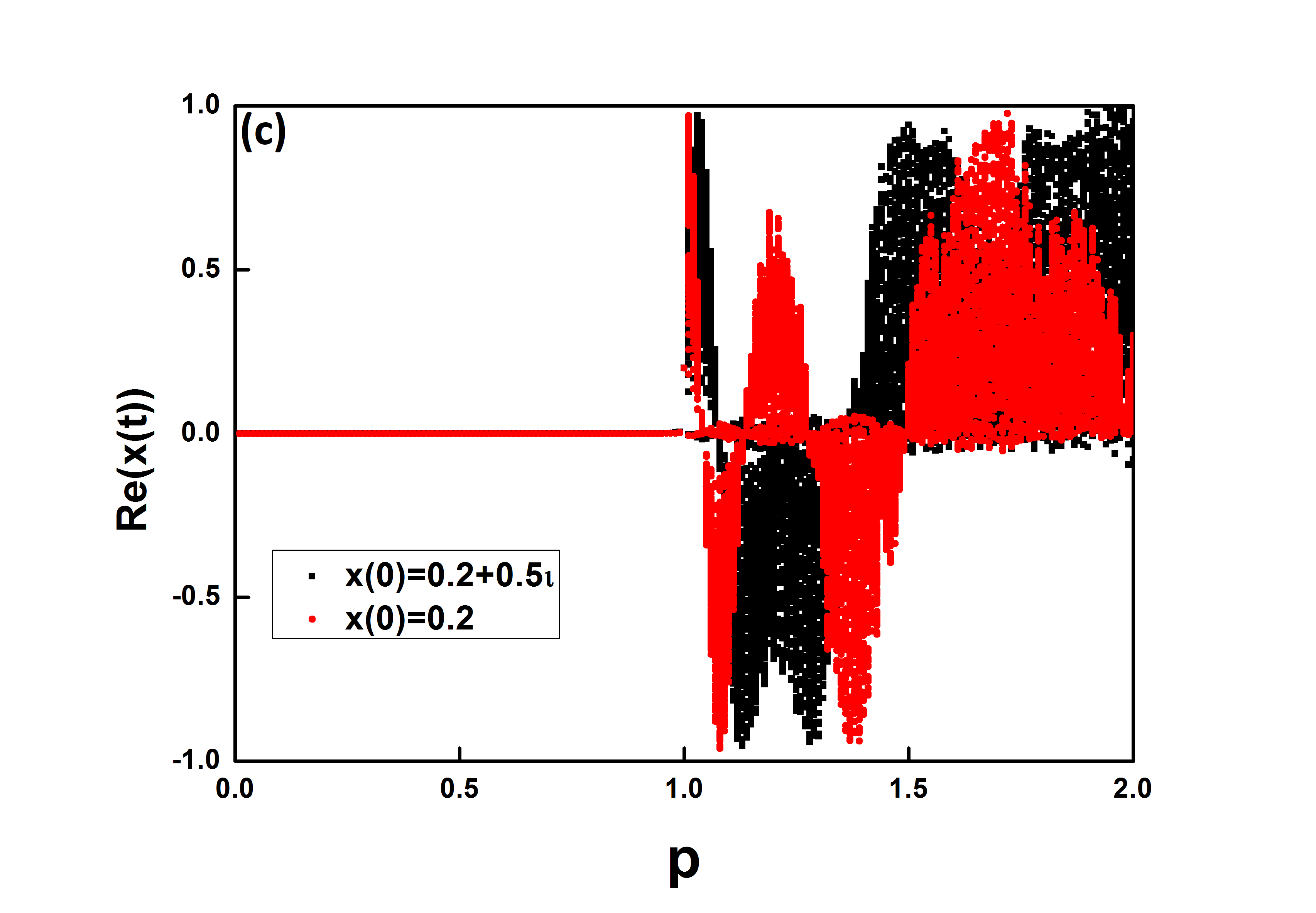
(c) Bernoulli map with $\alpha_{0}=0.8$ and $r=0.01$.

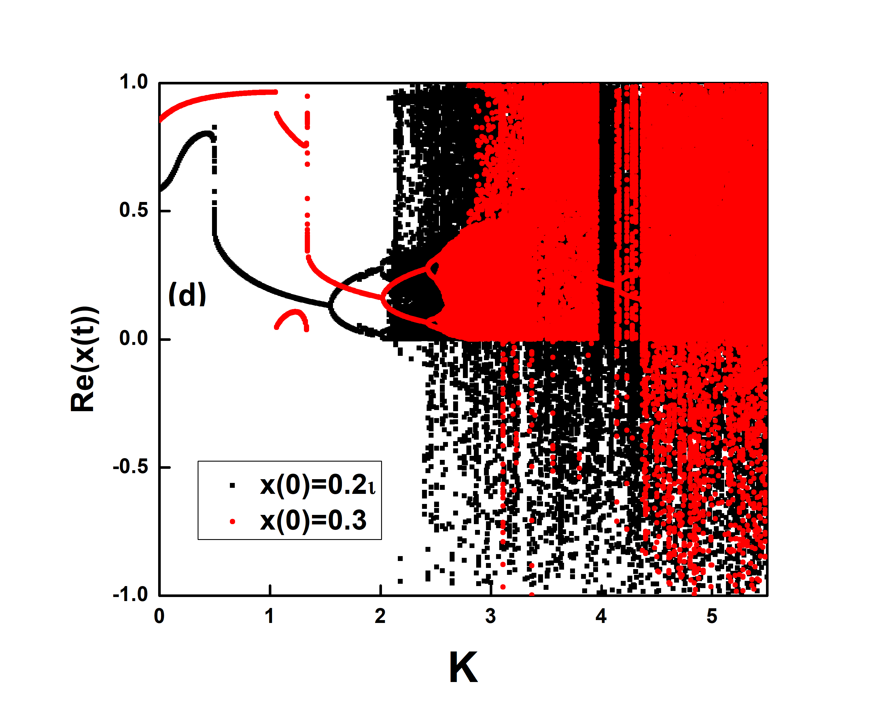
(d) Circle map with $\alpha_{0}=0.1$ and $r=0.1$.

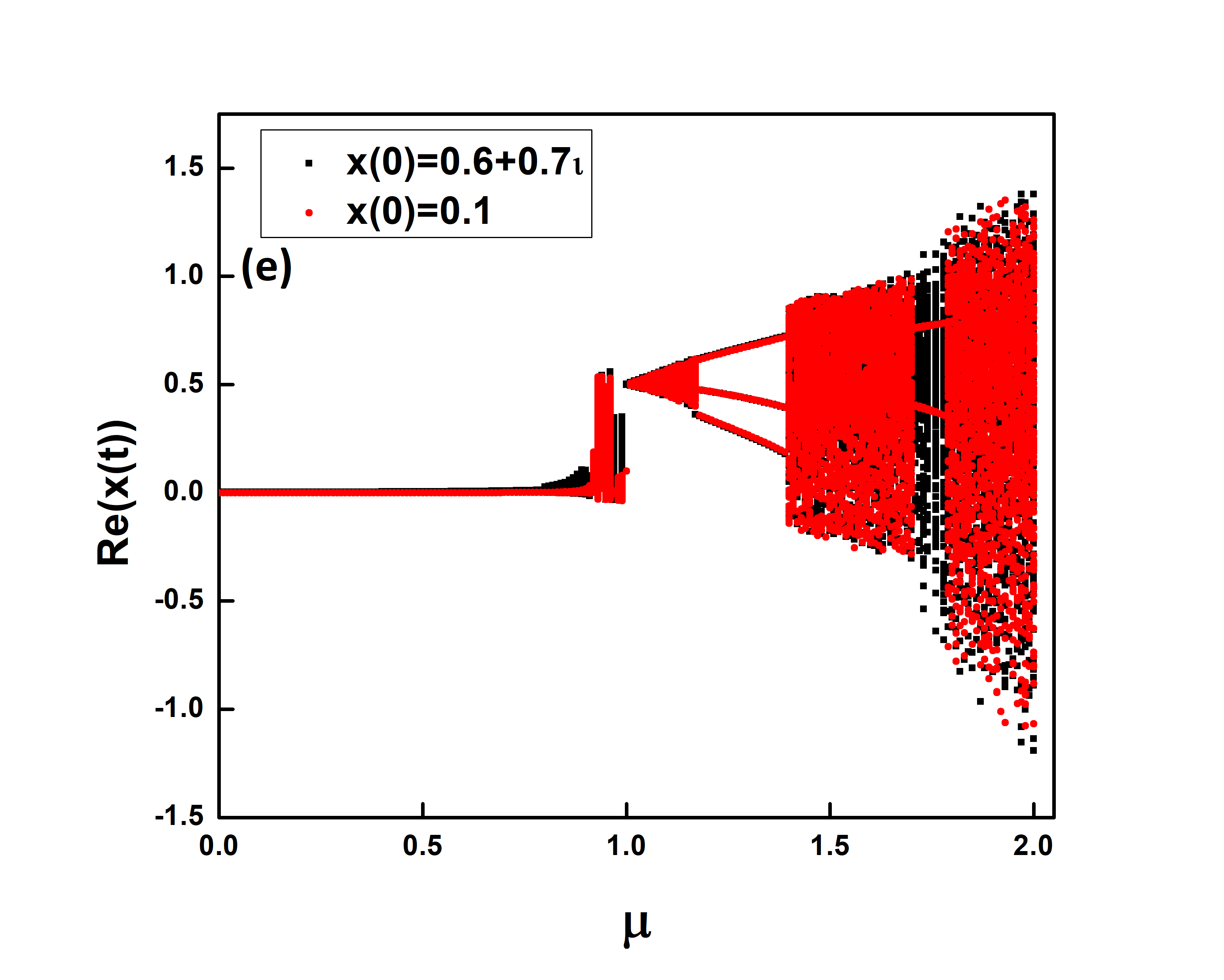
(e) Tent map with $\alpha_{0}=0.9$ and $r=0.5$.

Figure 9: Bifurcation diagrams for Lozi, Bernoulli, circle, and tent maps with two different initial conditions. Bifurcation diagrams are different indicating clear multistability in the systems.

If the map is continuous and differentiable, we have another observation. For real $\alpha$, i.e. for $r=0$ if there is a chaotic attractor for real order, the system goes to infinity for complex order even for $r=0.001$ and the bifurcation diagram shows a gap at these parameter values.

Apart from these maps, we also studied the cubic map in $1d$ rogers1983chaos given as:

$$x_{n+1}=ax_{n}^{3}+(1-a)x_{n}.$$

and Duffing map in $2d$ defines ouannas2020discrete :

$$x_{n+1}=y_{n},$$

$$y_{n+1}=-bx_{n}+ay_{n}-y_{n}^{3}.$$

The right-hand side of both these functions is an analytic function even if extended to a complex domain. We study the bifurcation diagrams for the real value of $\alpha$ with complex initial conditions and also maps of complex fractional order with a nonzero imaginary part. In either case, we do not see any chaos over a range of parameters studied. Thus, we have five cases (Gauss map, logistic map, Hénon map, Duffing map, and cubic map) where we have identical observations, namely, with complex initial and real fractional order or with complex fractional order, we do not observe any chaos over the range of parameters studied.

IV Results and Conclusions

We have studied $1d$ and $2d$ maps of complex fractional-order. In $2d$, we studied Lozi and Hénon maps of complex fractional-order. There are two possible generalizations and we have studied one of them in detail. We find that the chaos disappears completely when we introduce a small imaginary part to fractional-order $\alpha$ for the Hénon map. For the Lozi map, the chaos does not disappear completely and is indeed seen for some parameter values even for complex $\alpha$. We also note that the system has memory. Hénon map does not show pronounced multistability for complex order as seen in the original map and the bifurcation diagrams are almost independent of the initial conditions as long as the initial condition is stable. On the other hand, the Lozi map shows multistability and the asymptotic attractor is dependent on the initial conditions.

Thus, there are qualitative differences in the dynamical behavior of complex fractional-order Hénon and Lozi maps. We believe that these results are interesting and further studies are essential to understand the qualitative differences in behaviors of different maps of fractional-order.

We try to study the possibility of chaos in maps of complex fractional order. In $1d$, we studied logistic, tent, Gauss, circle, and Bernoulli maps. These studies along with studies in Hénon and Lozi maps suggest that maps that are continuous and differentiable lose chaos for real fractional order when the initial conditions are complex and they do not show chaos at all for any initial condition when the order is complex. Whereas, for maps that are discontinuous or non-differentiable we observe chaos for some initial conditions and parameter values. Multistability is seen for Lozi, Bernoulli, circle, and tent maps of complex fractional-order. Thus, multistability can be observed even $1d$ fractional difference equations of complex order if the underlying map is not analytic.

Often, non-linearity is necessary condition for chaos. In all the examples of complex order fractional difference equations we studied, it is striking that we required non-analyticity as well.

V Acknowledgement

PMG and DDJ thank DST-SERB for financial assistance (Ref. CRG/2020/003993). SB acknowledges the University of Hyderabad for Institute of Eminence-Professional Development Fund (IoE-PDF) by MHRD (F11/9/2019-U3(A)).

Author Credits: DDJ, PMG and SB contributed equally to the main paper. SB: Appendix A.

Appendix A Period-2 points in fractional order maps

Following the method outlined in edelman2014fractional , we compute the period-two points for logistic map.

Consider,

$$x(t)=x(0)+\frac{1}{\Gamma(\alpha)}\sum_{j=1}^{t}\frac{\Gamma(t-j+\alpha)}{\Gamma(t-j+1)}[f(x(j-1))-x(j-1)],$$ (6)

where, $0<\alpha<1$. If there exist the points $p$ and $q$ such that

$$\lim_{t\to\infty}x(2t)=p$$

and

$$\lim_{t\to\infty}x(2t+1)=q,$$

$p\neq q$ then we say that the system (6) has period-2 limit cycle. We have,

$$x(2t)=x(0)+\frac{1}{\Gamma(\alpha)}\sum_{j=1}^{2t}\frac{\Gamma(2t-j+\alpha)}{\Gamma(2t-j+1)}[f(x(j-1))-x(j-1)]$$

and

$$x(2t+1) = x(0)+\frac{1}{\Gamma(\alpha)}\sum_{j=1}^{2t+1}\frac{\Gamma(2t+1-j+\alpha)}{\Gamma(2t-j+2)}$$

$$\times[f(x(j-1))-x(j-1)].$$

Therefore,

$$x(2t) = x(0)+\sum_{k=0}^{t-1}\frac{\Gamma(2t-2k-1+\alpha)}{\Gamma(2t-2k)\Gamma(\alpha)}[f(x(2k))-x(2k)]$$ (7)

$$+\sum_{k=0}^{t-1}\frac{\Gamma(2t-2k-2+\alpha)}{\Gamma(2t-2k-1)\Gamma(\alpha)}$$

$$\times[f(x(2k+1))-x(2k+1)]$$

and

$$x(2t+1) = x(0)+\sum_{k=0}^{t}\frac{\Gamma(2t-2k+\alpha)}{\Gamma(2t-2k+1)\Gamma(\alpha)}[f(x(2k))-x(2k)]$$ (8)

$$+\sum_{k=0}^{t-1}\frac{\Gamma(2t-2k-1+\alpha)}{\Gamma(2t-2k)\Gamma(\alpha)}$$

$$\times[f(x(2k+1))-x(2k+1)].$$

Taking $\lim_{t\to\infty}$ and subtracting (8) from (7), we get

$$p-q = (f(p)-p)\lim_{t\to\infty}\left(\sum_{k=0}^{t-1}\frac{\Gamma(2t-2k-1+\alpha)}{\Gamma(2t-2k)\Gamma(\alpha)}\right.$$

$$\left.-\sum_{k=0}^{t}\frac{\Gamma(2t-2k+\alpha)}{\Gamma(2t-2k+1)\Gamma(\alpha)}\right)$$

$$+(f(q)-q)\lim_{t\to\infty}\left(\sum_{k=0}^{t-1}\frac{\Gamma(2t-2k-2+\alpha)}{\Gamma(2t-2k-1)\Gamma(\alpha)}\right.$$

$$\left.-\sum_{k=0}^{t-1}\frac{\Gamma(2t-2k-1+\alpha)}{\Gamma(2t-2k)\Gamma(\alpha)}\right)$$

The term $\sum_{k=0}^{t-1}\frac{\Gamma(2t-2k-2+\alpha)}{\Gamma(2t-2k-1)\Gamma(\alpha)}$ can be replaced with $\sum_{k=0}^{t}\frac{\Gamma(2t-2k+\alpha)}{\Gamma(2t-2k+1)\Gamma(\alpha)}$ if we put $k+1$ as $k$. Furthermore,

$$\lim_{t\to\infty}\left(\sum_{k=0}^{t-1}\frac{\Gamma(2t-2k-1+\alpha)}{\Gamma(2t-2k)\Gamma(\alpha)}-\sum_{k=0}^{t}\frac{\Gamma(2t-2k+\alpha)}{\Gamma(2t-2k+1)\Gamma(\alpha)}\right)$$

$$= \lim_{t\to\infty}\sum_{k=0}^{2t}(-1)^{k+1}\frac{\Gamma(2t-k+\alpha)}{\Gamma(2t-k+1)\Gamma(\alpha)}$$

$$= -\sum_{k=0}^{\infty}\begin{pmatrix}-\alpha\\ k\end{pmatrix}$$

$$= -2^{-\alpha}.$$

Therefore,

$$p-q=-[(f(p)-p)-(f(q)-q)]2^{-\alpha}.$$ (9)

Now adding (7) and (8) and taking $\lim_{t\to\infty}$ we get

$$p+q = 2x(0)+2[(f(p)-p)+(f(q)-q)]$$

$$\times[\lim_{t\to\infty}\sum_{k=0}^{2t}\frac{\Gamma(2t-k+\alpha)}{\Gamma(2t-k+1)\Gamma(\alpha)}].$$

Since the limit in the above equation tends to infinity, and all other terms are finite, we must have

$$p+q=f(p)+f(q).$$ (10)

Solving equations (9) and (10), we get

$$p = \left(\frac{1}{2}-\frac{2^{-\alpha-1}}{1-2^{-\alpha}}\right)f(p)+\left(\frac{1}{2}+\frac{2^{-\alpha-1}}{1-2^{-\alpha}}\right)f(q)$$

$$q = \left(\frac{1}{2}+\frac{2^{-\alpha-1}}{1-2^{-\alpha}}\right)f(p)+\left(\frac{1}{2}-\frac{2^{-\alpha-1}}{1-2^{-\alpha}}\right)f(q).$$

Let us consider the case of fractional order logistic map with period-2. Here, $f(x)=\lambda x(1-x)$, $0<\alpha<1$, $\lambda\in[0,4]$. Solving equation for (LABEL:eq11), we get the equilibrium points :

$$(p,q)=(0,0),$$

$$(p,q)=(\frac{\lambda-1}{\lambda},\frac{\lambda-1}{\lambda})$$

and

$$(p,q) = \left(\frac{(2^{\alpha}-1)+\lambda\pm\sqrt{(\lambda-(1-2^{\alpha}))(\lambda-(1+2^{\alpha}))}}{2\lambda},\right.$$

$$\left.\frac{(2^{\alpha}-1)+\lambda\mp\sqrt{(\lambda-(1-2^{\alpha}))(\lambda-(1+2^{\alpha}))}}{2\lambda}\right).$$

For $\alpha=1$

$$p = \frac{1+\lambda\pm\sqrt{(\lambda+1)(\lambda-3)}}{2\lambda}$$

$$q = \frac{1+\lambda\mp\sqrt{(\lambda+1)(\lambda-3)}}{2\lambda}.$$

which matches with integer order logistic map lakshmanan2012nonlinear .

Thus, for real values of roots there exists 2-limit cycle in the fractional order logistic map if $\lambda$ satisfies $(\lambda-(1-2^{\alpha}))(\lambda-(1+2^{\alpha}))>0,$ $0<\alpha<1$. That is if $\lambda>1+2^{\alpha}$ or $\lambda<1-2^{\alpha}$. Since $\lambda\in[0,4],$ we must have $\lambda\in[1+2^{\alpha},4],$ for 2-cycle.

References

- (1) G.-A. J. Francisco, R.-G. Juan, G.-C. Manuel, and R.-H. J. Roberto, “Fractional rc and lc electrical circuits,” Ingeniería, Investigación y Tecnología, vol. 15, no. 2, pp. 311–319, 2014.
- (2) K. Oprzedkiewicz, W. Mitkowski, and M. Rosół, “Fractional order model of the two dimensional heat transfer process,” Energies, vol. 14, no. 19, p. 6371, 2021.
- (3) F. Meral, T. Royston, and R. Magin, “Fractional calculus in viscoelasticity: an experimental study,” Communications in nonlinear science and numerical simulation, vol. 15, no. 4, pp. 939–945, 2010.
- (4) E. R. Love, “Fractional derivatives of imaginary order,” Journal of the London Mathematical Society, vol. 2, no. 2, pp. 241–259, 1971.
- (5) R. Andriambololona, R. Tokiniaina, and H. Rakotoson, “Definitions of complex order integrals and complex order derivatives using operator approach,” Int. J. Latest Res. Sci. Tech, vol. 1, pp. 317–323, 2012.
- (6) L. Campos, “On the solution of some simple fractional differential equations,” International Journal of Mathematics and Mathematical Sciences, vol. 13, no. 3, pp. 481–496, 1990.
- (7) N. Makris and M. Constantinou, “Models of viscoelasticity with complex-order derivatives,” Journal of engineering mechanics, vol. 119, no. 7, pp. 1453–1464, 1993.
- (8) N. Makris, “Complex-parameter kelvin model for elastic foundations,” Earthquake engineering & structural dynamics, vol. 23, no. 3, pp. 251–264, 1994.
- (9) A. Neamaty, M. Yadollahzadeh, and R. Darzi, “On fractional differential equation with complex order,” Progr. Fract. Differ. Appl, vol. 1, no. 3, pp. 223–227, 2015.
- (10) M. Ortigueira, “The complex order fractional derivatives and systems are non hermitian,” 2021.
- (11) J. L. Adams, T. T. Hartley, and C. F. Lorenzo, “Complex order-distributions using conjugated order differintegrals,” in Advances in Fractional Calculus, pp. 347–360, Springer, 2007.
- (12) T. M. Atanackovic, M. Janev, S. Konjik, S. Pilipovic, and D. Zorica, “Vibrations of an elastic rod on a viscoelastic foundation of complex fractional kelvin–voigt type,” Meccanica, vol. 50, no. 7, pp. 1679–1692, 2015.
- (13) N. Makris, “The imaginary counterpart of recorded motions,” Earthquake engineering & structural dynamics, vol. 23, no. 3, pp. 265–273, 1994.
- (14) T. M. Atanackovic and S. Pilipovic, “On a constitutive equation of heat conduction with fractional derivatives of complex order,” Acta Mechanica, vol. 229, no. 3, pp. 1111–1121, 2018.
- (15) T. T. Hartley, C. F. Lorenzo, and J. L. Adams, “Conjugated-order differintegrals,” in International Design Engineering Technical Conferences and Computers and Information in Engineering Conference, vol. 47438, pp. 1597–1602, 2005.
- (16) A. V. Tare, J. A. Jacob, V. A. Vyawahare, and V. N. Pande, “Design of novel optimal complex-order controllers for systems with fractional-order dynamics,” International Journal of Dynamics and Control, vol. 7, no. 1, pp. 355–367, 2019.
- (17) R. Sekhar, T. P. Singh, and P. Shah, “Complex order pi d design for surface roughness control in machining cnt al-mg hybrid composites,” Adv. Sci. Technol. Eng. Syst. J, vol. 5, pp. 299–306, 2020.
- (18) S. M. A. Pahnehkolaei, A. Alfi, and J. T. Machado, “Particle swarm optimization algorithm using complex-order derivative concept: A comprehensive study,” Applied Soft Computing, vol. 111, p. 107641, 2021.
- (19) C. M. Pinto, “Strange dynamics in a fractional derivative of complex-order network of chaotic oscillators,” International Journal of Bifurcation and Chaos, vol. 25, no. 01, p. 1550003, 2015.
- (20) C. M. Pinto and J. T. Machado, “Complex order biped rhythms,” International Journal of Bifurcation and Chaos, vol. 21, no. 10, pp. 3053–3061, 2011.
- (21) D. Vivek, O. Baghani, and K. Kanagarajan, “Theory of hybrid fractional differential equations with complex order,” Sahand Communications in Mathematical Analysis, vol. 15, no. 1, pp. 65–76, 2019.
- (22) C. M. Pinto and A. R. Carvalho, “Fractional complex-order model for hiv infection with drug resistance during therapy,” Journal of Vibration and Control, vol. 22, no. 9, pp. 2222–2239, 2016.
- (23) C. M. Pinto and J. T. Machado, “Complex-order forced van der pol oscillator,” Journal of Vibration and Control, vol. 18, no. 14, pp. 2201–2209, 2012.
- (24) C. Pinto and J. Tenreiro Machado, “Complex order van der pol oscillator,” Nonlinear Dynamics, vol. 65, no. 3, pp. 247–254, 2011.
- (25) A. K. Singh, V. K. Yadav, and S. Das, “Synchronization between fractional order complex chaotic systems with uncertainty,” Optik, vol. 133, pp. 98–107, 2017.
- (26) C. Luo and X. Wang, “Chaos in the fractional-order complex lorenz system and its synchronization,” Nonlinear Dynamics, vol. 71, no. 1, pp. 241–257, 2013.
- (27) X. Gao and J. Yu, “Chaos in the fractional order periodically forced complex duffing’s oscillators,” Chaos, Solitons & Fractals, vol. 24, no. 4, pp. 1097–1104, 2005.
- (28) E. Ott, “Chaos in dynamical systems,” Chaos in Dynamical Systems-2nd Edition, p. 490, 2002.
- (29) T. Shinbrot, C. Grebogi, J. A. Yorke, and E. Ott, “Using small perturbations to control chaos,” nature, vol. 363, no. 6428, pp. 411–417, 1993.
- (30) M. Holm, The theory of discrete fractional calculus: Development and application. The University of Nebraska-Lincoln, 2011.
- (31) F. Atici and P. Eloe, “Initial value problems in discrete fractional calculus,” Proceedings of the American Mathematical Society, vol. 137, no. 3, pp. 981–989, 2009.
- (32) F. M. Atici and P. W. Eloe, “A transform method in discrete fractional calculus,” International Journal of Difference Equations, vol. 2, no. 2, 2007.
- (33) F. M. Atıcı and P. W. Eloe, “Gronwall’s inequality on discrete fractional calculus,” Computers & Mathematics with Applications, vol. 64, no. 10, pp. 3193–3200, 2012.
- (34) P. M. Gade and S. Bhalekar, “On fractional order maps and their synchronization,” Fractals, vol. 29, no. 06, p. 2150150, 2021.
- (35) S. Bhalekar, P. M. Gade, and D. Joshi, “Stability and dynamics of complex order fractional difference equations,” Chaos, Solitons & Fractals, vol. 158, p. 112063, 2022.
- (36) T. Bohr, P. Bak, and M. H. Jensen, “Transition to chaos by interaction of resonances in dissipative systems. ii. josephson junctions, charge-density waves, and standard maps,” Physical review A, vol. 30, no. 4, p. 1970, 1984.
- (37) J. R. Tredicce, F. T. Arecchi, G. L. Lippi, and G. P. Puccioni, “Instabilities in lasers with an injected signal,” JOSA B, vol. 2, no. 1, pp. 173–183, 1985.
- (38) D. H. DeTienne, G. R. Gray, G. P. Agrawal, and D. Lenstra, “Semiconductor laser dynamics for feedback from a finite-penetration-depth phase-conjugate mirror,” IEEE journal of quantum electronics, vol. 33, no. 5, pp. 838–844, 1997.
- (39) A. Tufaile and J. C. Sartorelli, “The circle map dynamics in air bubble formation,” Physics Letters A, vol. 287, no. 1-2, pp. 74–80, 2001.
- (40) E. N. Lorenz, “Deterministic nonperiodic flow,” Journal of atmospheric sciences, vol. 20, no. 2, pp. 130–141, 1963.
- (41) M. Hénon, “A two-dimensional mapping with a strange attractor,” in The theory of chaotic attractors, pp. 94–102, Springer, 1976.
- (42) Z. Elhadj, Lozi Mappings: Theory and Applications. CRC Press, 2013.
- (43) R. Lozi, “Un attracteur étrange (?) du type attracteur de hénon,” Le Journal de Physique Colloques, vol. 39, no. C5, pp. C5–9, 1978.
- (44) A. Luo and V. Afraimovich, Long-range Interactions, Stochasticity and Fractional Dynamics: Dedicated to George M. Zaslavsky (1935—2008). Nonlinear Physical Science, Springer Berlin Heidelberg, 2011.
- (45) Y. Liu, “Discrete chaos in fractional hénon maps,” International Journal of nonlinear science, vol. 18, no. 3, pp. 170–175, 2014.
- (46) T. Hu, “Discrete chaos in fractional hénon map,” Applied Mathematics, vol. 2014, 2014.
- (47) L. Jouini, A. Ouannas, A.-A. Khennaoui, X. Wang, G. Grassi, and V.-T. Pham, “The fractional form of a new three-dimensional generalized hénon map,” Advances in Difference Equations, vol. 2019, no. 1, pp. 1–12, 2019.
- (48) Y. Liu, “Chaotic synchronization between linearly coupled discrete fractional hénon maps,” Indian Journal of Physics, vol. 90, no. 3, pp. 313–317, 2016.
- (49) A.-A. Khennaoui, A. Ouannas, S. Bendoukha, G. Grassi, R. P. Lozi, and V.-T. Pham, “On fractional–order discrete–time systems: Chaos, stabilization and synchronization,” Chaos, Solitons & Fractals, vol. 119, pp. 150–162, 2019.
- (50) O. Megherbi, H. Hamiche, S. Djennoune, and M. Bettayeb, “A new contribution for the impulsive synchronization of fractional-order discrete-time chaotic systems,” Nonlinear Dynamics, vol. 90, no. 3, pp. 1519–1533, 2017.
- (51) K. S. Miller and B. Ross, “Fractional difference calculus,” in Proceedings of the international symposium on univalent functions, fractional calculus and their applications, pp. 139–152, 1988.
- (52) F. M. Atıcı and S. Şengül, “Modeling with fractional difference equations,” Journal of Mathematical Analysis and Applications, vol. 369, no. 1, pp. 1–9, 2010.
- (53) A. Deshpande and V. Daftardar-Gejji, “Chaos in discrete fractional difference equations,” Pramana, vol. 87, no. 4, pp. 1–10, 2016.
- (54) A. Wolf, J. B. Swift, H. L. Swinney, and J. A. Vastano, “Determining lyapunov exponents from a time series,” Physica D: nonlinear phenomena, vol. 16, no. 3, pp. 285–317, 1985.
- (55) S. Kodba, M. Perc, and M. Marhl, “Detecting chaos from a time series,” European journal of physics, vol. 26, no. 1, p. 205, 2004.
- (56) M. Perc, “lyapmax.exe.” http://www.matjazperc.com/ejp/lyapmax.exe, 2005.
- (57) T. D. Rogers and D. C. Whitley, “Chaos in the cubic mapping,” Mathematical Modelling, vol. 4, no. 1, pp. 9–25, 1983.
- (58) A. Ouannas, A.-A. Khennaoui, S. Momani, and V.-T. Pham, “The discrete fractional duffing system: Chaos, 0–1 test, c 0 complexity, entropy, and control,” Chaos: An Interdisciplinary Journal of Nonlinear Science, vol. 30, no. 8, p. 083131, 2020.
- (59) M. Edelman, “Fractional maps as maps with power-law memory,” in Nonlinear dynamics and complexity, pp. 79–120, Springer, 2014.
- (60) M. Lakshmanan and S. Rajaseekar, Nonlinear dynamics: integrability, chaos and patterns. Springer Science & Business Media, 2012.