A Bayesian Variational Principle for Dynamic Self Organizing Maps

Abstract

We propose organisation conditions that yield a method for training SOM with adaptative neighborhood radius in a variational Bayesian framework. This method is validated on a non-stationary setting and compared in an high-dimensional setting with an other adaptative method.

1 Introduction

Self Organizing Maps (SOM, [1]) is a biologically inspired unsupervized vector quantization method for data modelization and visualization. A map is made of a collection of weights $\left\{w_{z}\right\}_{z}$ indexed by a discrete collection of points $z\in\left\{z_{1},z_{2},\ldots,z_{n}\right\}$. The weights (or neurons) are meant to modelize some observation random variable $\boldsymbol{x}$. The points are usually regularly placed on a two dimensional grid. In this context, the SOM objective is to find representative weights with a well organized response to stimuli i.e. weights specialize their response to some kind of stimuli and weigths close in the grid space are close in the observation space.

The original way to train such SOM is with Kohonen’s iterations. Despite its simplicity, they require a time dependant neighborhood function whose neighborhood radius (or temperature) strictly decreases towards zero during training. In [2] and [3], heuristics are proposed in a non-probabilistic framework to adapt this temperature. They lead to “dynamic” SOM algorithms that are able to track non-stationary datasets. In [4], the variational EM framework is used to design a cost function for the SOM but the temperature parameter is still decreased as in Kohonen. In [5], the topologically preserving properties of the map stems from the basis function regularity. Hence those basis functions have to be carefully chosen and their number must typically grow exponentially with the observation space dimension.

We propose quantitative organization conditions that lead to an adaptative temperature choice in a variational Bayesian framework. High dimensional experiments show that our method is less sensitive to elasticity and outperforms that of [3].

2 Evidence Lower BOund

In [4], the neighborhood function is interpreted as the variational posterior in a Expectation-Minization (EM, [6]) procedure. Therefore, they propose to minimize the following (opposite) ELBO to train SOMs

$$F\left(\rho,\theta\right) =\int\int\ln\left(\frac{q_{\boldsymbol{z}|\boldsymbol{x}}^{\rho}}{p_{\boldsymbol{x},\boldsymbol{z}}^{\theta}}\right)q_{\boldsymbol{z}|\boldsymbol{x}}^{\rho}\mathrm{d}\boldsymbol{z}p_{\boldsymbol{x}}\mathrm{d}\boldsymbol{x}$$ (1)

$$=\underbrace{\int\mathcal{D}\left(q_{\boldsymbol{z}|\boldsymbol{x}}^{\rho},p_{\boldsymbol{z}|\boldsymbol{x}}^{\theta}\right)p_{\boldsymbol{x}}\mathrm{d}\boldsymbol{x}}_{\text{organization}}+\underbrace{\mathcal{D}\left(p_{\boldsymbol{x}},p_{\boldsymbol{x}}^{\theta}\right)}_{\text{modelization}},$$ (2)

where, the data true density is $p_{\boldsymbol{x}}$ and the discrete latent variable is $\boldsymbol{z}$. The complete data model $p_{\boldsymbol{x},\boldsymbol{z}}^{\theta}\propto e^{-\frac{1}{2}\left|\frac{\boldsymbol{x}-w_{\boldsymbol{z}}}{\sigma}\right|^{2}}$ is chosen Gaussian and the variational (amortized, homoskedastic) posterior $q_{\boldsymbol{z}|\boldsymbol{x}}^{\rho}\propto e^{-\frac{1}{2}\left|\frac{\boldsymbol{z}-\mu_{\boldsymbol{x}}}{\lambda}\right|^{2}}$ as well. Their parameters are respectively $\theta=\left\{z\mapsto w_{z},\sigma\right\},\rho=\left\{x\mapsto\mu_{x},\lambda\right\}$. The decomposition in the second equation reveals a modelization term that is the Kullback-Leibler (KL) divergence between the data density and the model marginal. As well as an other term that is the expected KL divergence between the variational posterior and the model posterior (or response to stimulus). The core idea is to choose the variational posterior organized so that this term will favor organized posterior models.

3 Organization conditions

Given an observation $\boldsymbol{x}$, let $w_{z^{*}_{\boldsymbol{x}}}$ be its closest weight. If the distance to this weight $\left|w_{z^{*}_{\boldsymbol{x}}}-w_{\boldsymbol{z}}\right|$ in observation space is increasing with the distance $\left|z^{*}_{\boldsymbol{x}}-\boldsymbol{z}\right|$ in point space then the map is organized. This mean that if the Bayesian posterior (or response) $p_{\boldsymbol{z}|\boldsymbol{x}}^{\theta}\propto e^{-\frac{1}{2}\left|\frac{\boldsymbol{x}-w_{\boldsymbol{z}}}{\sigma}\right|^{2}}$ is plotted as a function of $\boldsymbol{z}$, it would be strictly decreasing around its maximum. This is illustrated in Fig. 1. Hence we propose the following organization conditions:

1:

The response $p_{\boldsymbol{z}|\boldsymbol{x}}^{\theta}$ has a dominating mode at $z_{\boldsymbol{x}}^{*}=\arg\min_{z}\left|\boldsymbol{x}-w_{z}\right|$.

2:

$\left|w_{\boldsymbol{z}}-w_{z^{*}_{\boldsymbol{x}}}\right|=\frac{1}{\eta}\left|\boldsymbol{z}-z^{*}_{\boldsymbol{x}}\right|$ when $\boldsymbol{z}$ is in the neighborhood of $z^{*}_{\boldsymbol{x}}$.

The first condition ensures that each weight specializes on some kind of stimulus. The second one ensures that the weight distance is proportional to the point distance by a scale $\eta$. In other words, the map preserves distances locally.

3.1 Variational posterior selection

We now choose $\rho$ such that the variational posterior $q_{\boldsymbol{z}|\boldsymbol{x}}^{\rho}$ verifies the organization conditions. Because the variational posterior has a unique mode at $\mu_{\boldsymbol{x}}$, choosing

$$\mu_{\boldsymbol{x}}=z^{*}_{\boldsymbol{x}}$$

(like Kohonen does) favors reponses that verifiy the first order organization condition. We also have,

$$-\ln p_{\boldsymbol{z}|\boldsymbol{x}}^{\theta}=\frac{1}{\sigma^{2}}\langle\boldsymbol{x}-w_{z^{*}_{\boldsymbol{x}}}|w_{z^{*}_{\boldsymbol{x}}}-w_{\boldsymbol{z}}\rangle+\frac{1}{2}\left|\frac{w_{\boldsymbol{z}}-w_{\boldsymbol{z}^{*}_{\boldsymbol{x}}}}{\sigma}\right|^{2}+c,$$

whith $c$ being a constant w.r.t $\boldsymbol{z}$. Because $z^{*}_{\boldsymbol{x}}$ is a mode, the scalar product is almost null for $\boldsymbol{z}$ in the neighborhood of $z^{*}_{\boldsymbol{x}}$. Therefore, if $\boldsymbol{z}$ is in the neighborhood of $z_{\boldsymbol{x}}^{*}$, the organization term will favor responses such that $\left|\frac{w_{z}-w_{z^{*}}}{\sigma}\right|\simeq\left|\frac{z-z^{*}}{\lambda}\right|$ . Thus choosing

$$\lambda=\eta\sigma,$$

favors responses satisfying the second organization condition.

3.2 Stochastic Gradient calculations

With the previous selection for $\rho$ ($\mu_{\boldsymbol{x}}=z^{*}_{\boldsymbol{x}},\lambda=\eta\sigma$), the objective $F$ in Eq.(1) only depends on $\theta$. Algorithm 1 computes a stochastic approximation over $\boldsymbol{x}$ of its derivatives along $\theta=\left\{w,\sigma\right\}$ assuming that $z^{*}_{\boldsymbol{x}}=\arg\min_{z}\left|\boldsymbol{x}-w_{\boldsymbol{z}}\right|$ has no gradient. Then any stochastic gradient descent method can be used to minimize $F$. A Python implementation is available at: github.com/anthony-Neo/VDSOM.

Data: $\eta$: elasticity;

$Z=\left\{z_{i}\right\}_{1\leq i\leq n}$: grid points;

$\left\{w_{z}\right\}_{z\in Z},\sigma$: weights and variance;

$x,m$: observation and observation space dimension

Result: $g_{\sigma},\,\left\{g_{w_{z}}\right\}_{z\in Z}$ the stochastic gradients of $F$

1 for $z,y\in Z\times Z$ do

2       $d_{z,y}:=\left|z-y\right|^{2}$;

3       $f_{z}:=\left|x-w_{z}\right|^{2}$;

4       $\ln p_{z}:=-m\ln\sigma-\frac{f_{z}}{2\sigma^{2}}$;

5$z^{*}:=\arg\min_{z}f_{z}$;

6 $q_{z}:=\textnormal{{softmax(}}\textnormal{\emph{$-\frac{d_{z,z^{*}}}{2\eta^{2}\sigma^{2}}$}}\textnormal{{)}}$;

7 $d^{*}:=\sum_{z}d_{z,z^{*}}\times q_{z}$;

8 $g_{\sigma}:=\frac{m}{\sigma}+\frac{1}{\sigma^{3}}\sum_{z}\left[\eta\left(1+\ln q_{z}-\ln p_{z}\right)\left(d_{z,z^{*}}-d^{*}\right)-f_{z}\right]q_{z}$;

9 for $z\in Z$ do

10       $g_{w_{z}}:=-\frac{q_{z}}{\sigma^{2}}\left(x-w_{z}\right)$;

Algorithm 1 Stochastic gradient of $F$

4 Numerical Experiments

4.1 Non-stationary distributions

We used $8\times 7500$ steps of the Adam stochastic optimizer [7] with a learning rate of $\alpha=10^{-3}$. The variance parameter is initialized at $\sigma_{0}=5$ and the initial weights sample a normal Gaussian. The grid is a $15\times 15$ node lattice with regularly spaced points between $-1,1$ and the elasticity parameter is $\eta=1$. During the first half of the iterations, the “moons” data set from sci-kit [8] learn is sampled. Then, during the second half, the “circles” data set is sampled. Step $0$ and each $7500$ steps, data, weights and edges are plotted in Fig. 3 from the upper left corner to the lower right one. We see that the SOM tracks the changing data set, it correctly fits the observation density (rather than its support as in [3]) and it preserves the grid neighborhood. In Fig. 3, the log standard deviation $\sigma$ and the log distorsion (mean over the samples of the min squared distance with the weights, cf [3]) are plotted against time. Spikes appear half time which means that the method detects the change in data and adapts neighborhood radius accordingly.

4.2 High-dimensional distributions

The DSOM algorithm of [3] is compared to ours (VDSOM) on $20000$ samples of the MNIST Fashion dataset on a $10\times 10$ toroidal grid. DSOM uses a learning rate of $\alpha=10^{-3}$ while VDSOM uses the same configuration as before. In Fig. 5, the distorsion is plotted as a function of the elasticity $\eta$. VDSOM outperforms DSOM while being less sensitive. In Fig. 5, the weights of both methods trained with their respective optimal elasticity are displayed on a grid. Note that some of the DSOM weights are noise while this is not the case for VDSOM. VDSOM weights also seem less blurred.

5 Conclusion

We proposed organisation conditions that yield a method for training SOM with adaptative neighborhood radius in a variational Bayesian framework. This method has been validated in a non-stationary setting and compared in an high-dimensional setting with an other adaptative method.

(a) This SOM is well organized since the posterior is decreasing as we move away from its maximum.

(b) This SOM is not well organized since the posterior is not decreasing as we move away from a maximum.

Figure 1: On the left part of each subfigure, an observation $x$ and a SOM with 1D neighborhood vizualised in its 2D observation space. On the right part, the graph of its posterior.

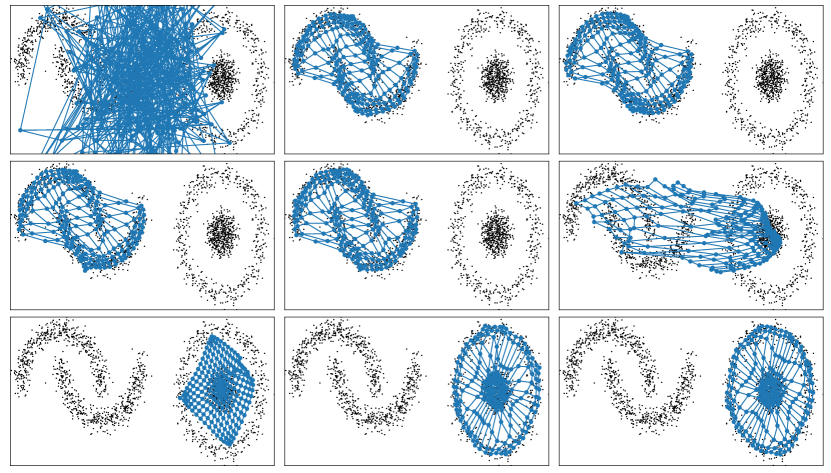
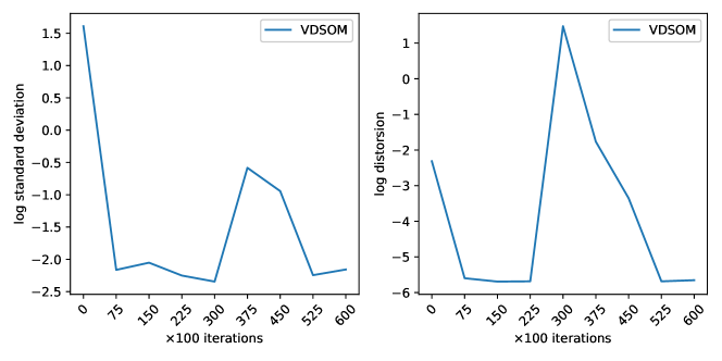
Figure 2: Visualization of the map during the iterations, on a changing dataset

Figure 3: Graphs of $\sigma$ and distorsion during the iterations, on a changing dataset

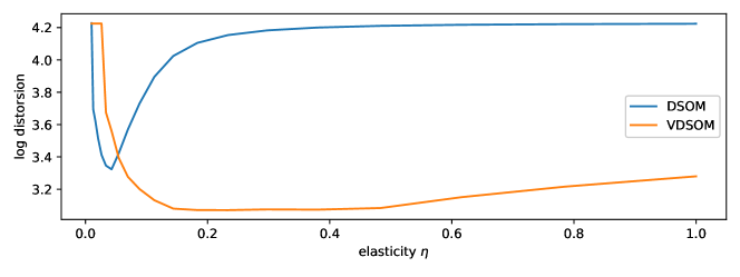
Figure 4: sensitivity

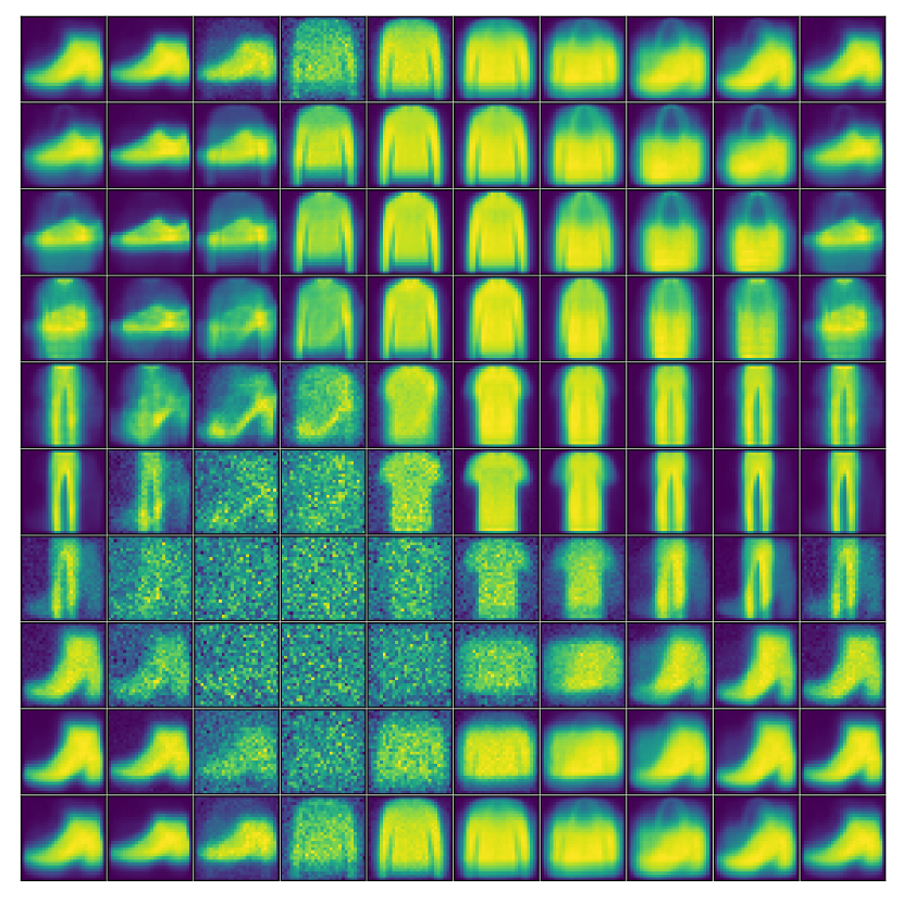
(a) DSOM

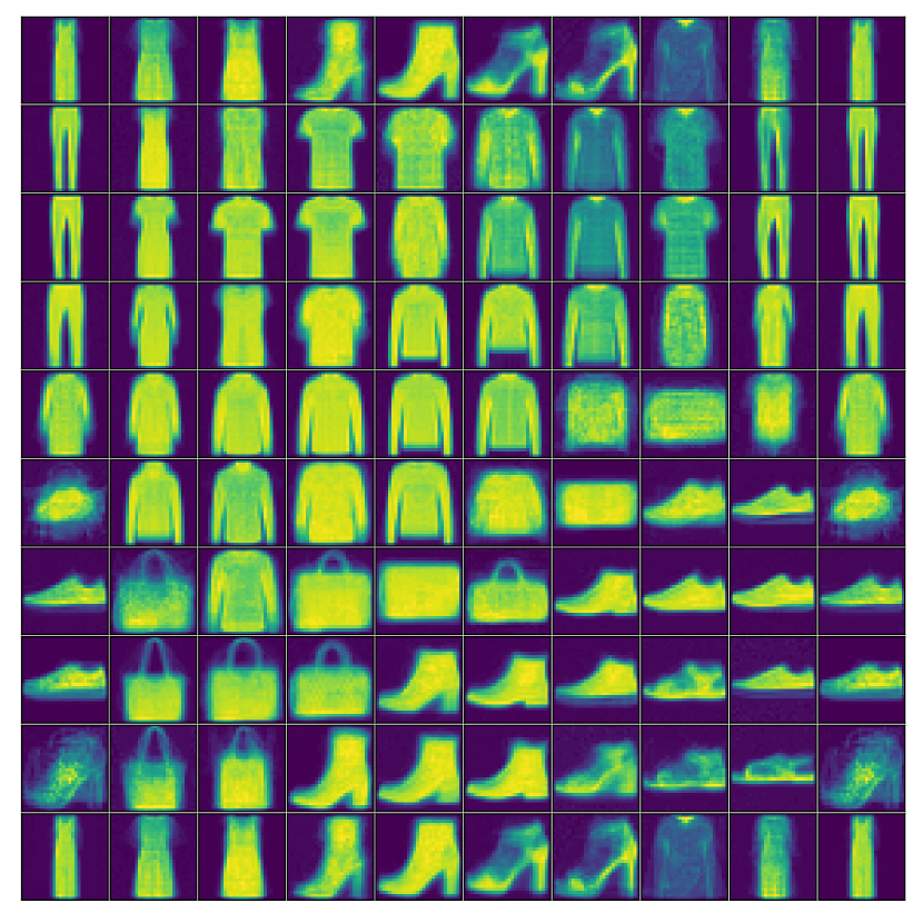
(b) VDSOM

Figure 5: Weights on the 2D grid

References

- [1] T. Kohonen. Self-Organizing Maps. Springer Series in Information Sciences. Springer Berlin Heidelberg, 2012.
- [2] Erik Berglund and Joaquin Sitte. The parameterless self-organizing map algorithm. IEEE transactions on neural networks / a publication of the IEEE Neural Networks Council, 17:305–16, 04 2006.
- [3] Nicolas Rougier and Yann Boniface. Dynamic self-organising map. Neurocomputing, 74(11):1840–1847, 2011.
- [4] Jakob J Verbeek, Nikos Vlassis, and Ben JA Kröse. Self-organizing mixture models. Neurocomputing, 63:99–123, 2005.
- [5] Christopher M Bishop, Markus Svensén, and Christopher KI Williams. Gtm: The generative topographic mapping. Neural computation, 10(1):215–234, 1998.
- [6] C.M. Bishop. Pattern Recognition and Machine Learning. Information Science and Statistics. Springer, 2006.
- [7] Diederik P Kingma and Jimmy Ba. Adam: A method for stochastic optimization. arXiv preprint arXiv:1412.6980, 2014.
- [8] F. Pedregosa, G. Varoquaux, A. Gramfort, V. Michel, B. Thirion, O. Grisel, M. Blondel, P. Prettenhofer, R. Weiss, V. Dubourg, J. Vanderplas, A. Passos, D. Cournapeau, M. Brucher, M. Perrot, and E. Duchesnay. Scikit-learn: Machine learning in Python. Journal of Machine Learning Research, 12:2825–2830, 2011.