Robust Motion Averaging for Multi-view Registration of Point Sets Based
Maximum Correntropy Criterion

Abstract

As an efficient algorithm to solve the multi-view registration problem, the motion averaging (MA) algorithm has been extensively studied and many MA-based algorithms have been introduced. They aim at recovering global motions from relative motions and exploiting information redundancy to average accumulative errors. However, one property of these methods is that they use Guass-Newton method to solve a least squares problem for the increment of global motions, which may lead to low efficiency and poor robustness to outliers. In this paper, we propose a novel motion averaging framework for the multi-view registration with Laplacian kernel-based maximum correntropy criterion (LMCC). Utilizing the Lie algebra motion framework and the correntropy measure, we propose a new cost function that takes all constraints supplied by relative motions into account. Obtaining the increment used to correct the global motions, can further be formulated as an optimization problem aimed at maximizing the cost function. By virtue of the quadratic technique, the optimization problem can be solved by dividing into two subproblems, i.e., computing the weight for each relative motion according to the current residuals and solving a second-order cone program problem (SOCP) for the increment in the next iteration. We also provide a novel strategy for determining the kernel width which ensures that our method can efficiently exploit information redundancy supplied by relative motions in the presence of many outliers. Finally, we compare the proposed method with other MA-based multi-view registration methods to verify its performance. Experimental tests on synthetic and real data demonstrate that our method achieves superior performance in terms of efficiency, accuracy and robustness.

I Introduction

Point set registration is a fundamental but challenging methodology, which is widely used in the fields of computer vision, computer graphics, and robotics, for 3D model reconstruction, simultaneous localization and mapping (SLAM), cultural heritage management, etc. With the development of 3D scanning devices, it has become easy to obtain point cloud representations of real-world models or scenes. However, a non-negligible fact is that due to the occlusion of scenes or objects and the limited scanning field of view, most scanning devices only capture partial point clouds at one time. Thus, in order to accurately recover the whole model or scene from a sequence of scans captured from different viewpoints, point set registration problem arises. It aims at determining the rigid transformations of these scans between a given centered-frame so as to align multi-view scans into an entire model or scene. Depending on the amount of input point clouds, point set registration can be divided into two problems, namely, pair-wise registration and multi-view registration [1].

In the past few decades, several methods have been proposed to solve the pair-wise registration problem and these methods can be classified into two categories, i.e., coarse registration methods and fine registration methods [1]. For the former, the feature-based methods are the most popular and have been extensively studied, which usually contain three significant steps: extracting geometric features composed of keypoints and corresponding descriptors, matching features to obtain the correspondences, and estimating the rigid transformation based on the correspondences. Usually, the performance of the feature-based methods is affected by point density, outliers, and overlapping percentage [2]. The deep learning-based methods, widely studied in recent years, are likely to overcome these drawbacks [1]. Compared to coarse registration, fine registration can achieve more accurate results for pair-wise registration. The ICP-based algorithms, among these fine registration methods, are the ones studied most intensively. By alternately searching the nearest correspondences from the target points for each source point and estimating and updating the rigid transformation until convergence, the ICP-based algorithms achieve an accurate registration result [3]. Since the original ICP algorithm [3] minimizes the squared distances of correspondences, it is not robust to outliers and ignores the structural information of the point set. Thus, many variants [4, 5, 6] of ICP are proposed to improve the robustness to outliers, efficiency, and accuracy. For example, point-to-plane metric [5], plane-to-plane metric [6], and symmetric point-to-plane metric [7] are proposed to take advantage of the structural information. In addition, good initializations are necessary for ICP-based methods to guarantee efficiency and the avoidance of local minima.

Compared to pair-wise registration, multi-view registration is more difficult due to many parameters needed to be determined. For solving multi-view registration problems, the most common methods are sequential pair-wise registration-based methods and joint registration-based methods [1]. For the former, a registration-and-integration strategy is widely adopted and the pair-wise registration algorithms play important roles in the registration process. For example, Chen et al. [9] repeatedly registered two scans with the utilization of ICP and integrated a new scan until all of the scans are translated into the whole model. In addition, treating the multi-view registration problem as a graph optimization issue, Weber et al. [10] estimated the overlap of each scan pair as the weight of the corresponding edge so as to establish a weighted graph with fully connected edges. Then, a minimum spanning tree (MST) can be constructed by utilizing the Kruskal algorithm [11], and finally, the rigid transformation of each node can be sequentially estimated by performing a breadth-depth search on the resulting MST. Furthermore, Zhu et al. [12] proposed a dual criterion to judge the reliability of pair-wise registration results and picked out the relatively reliable pairs to construct the spanning tree. Although sequential pair-wise registration-based methods are efficient, they neglect the relevance of each scan and do not exploit information redundancy in the point set, resulting in the accumulated error.

To reduce the error, joint registration-based methods have been developed in recent years. These methods fall into two main categories, i.e., the expectation maximization (EM)-based algorithms [13][14] and motion averaging (MA)-based algorithms [8][15, 16, 17]. The former aligns all scans based on probabilistic models, while the latter recovers global motions from a set of relative motions so as to exploit information redundancy and further average the registration errors. In addition, to the best of our knowledge, these methods share a common drawback that they are local convergent algorithms and a good initialization is necessary for them to achieve accurate registration results. By virtue of the Lei algebraic property of the rigid-body motion, Govindu et al. [15] first proposed the motion averaging (MA) method. MA takes an initial global motions and a set of relative motions of scan pairs as input. Different from the sequential pair-wise registration-based methods, MA takes advantage of information redundancy in relative motions. By utilizing a $\ell_{2}$-based optimization considering all relative motions, MA can efficiently average the accumulative errors to each scan. However, $\ell_{2}$-based measure is sensitive to outliers, resulting in poor robustness. To improve the robustness, Govindu [18] further treated the outlier rejection problem as a graph optimization issue. Although the proposed method eliminates the effect of outliers, the Random Sample Consensus introduced in this method is very time-consuming. To reduce the outliers ratio of relative motions, Li et al. [16] proposed an improved technique for MA-based multi-view registration, known as MATrICP. In this technique, the overlapping percentage of each scan pair is roughly estimated, and then these scan pairs whose overlapping percentages are larger than a pre-set threshold are picked out. Finally, MATrICP applies TrICP algorithm to obtain the relative motions corresponding to these scan pairs as the input of MA. Inspired by MATrICP, Guo et al. [17] proposed a weighted motion averaging (WMA) algorithm for multi-view registration, called WMAA. Considering the reliability and accuracy of each relative motion, WMAA takes the overlapping percentage determined by TrICP algorithm, as the corresponding weight of each scan pair. WMAA is more likely to return desired registration results than MA [8]. However, similar to most of the variants of ICP, the accuracy of TrICP algorithm is also highly dependent on good initializations and easily traps into local minima. In addition, Arrigoni et al. [19] introduced the low-rank and sparse (LRS) matrix decomposition to recover global motions from a set of relative motions, and therefore, LRS can be cast as another MA algorithm. Although LRS achieves superior performance in terms of efficiency in MA-based multi-view registration, the performance of LRS is more susceptible to the sparsity of view-graph than related methods [20]. Additionally, assuming all the points are drawn from a central Gaussian mixture model (GMM), Evangelidis and Horaud [13] proposed an EM-based method, called JRMPC, which casts multi-view registration into a clustering problem. Furthermore, Zhu et al. [14] proposed the EMPMR method by assuming that each data point is generated from one unique GMM, where its corresponding points in other point sets are regarded as Gaussian centroids.

In recent years, a method, called correntropy, is introduced to improve the robustness to outliers in information-theoretic learning [21][22]. Nowadays, the method is also introduced to the field of computer vision, for example, based on MCC, He et al. [23] proposed a correntropy framework for robust face recognition. Zhu et al. [8] further combined MCC with the motion averaging algorithm, and proposed a robust framework for multi-view registration (MCC-MA). Specifically, by introducing Gaussian kernel-based MCC, MCC-MA reformulates the MA as a half-quadratic optimization problem that can be readily solved by the traditional iterative method introduced in [15, 16, 17]. MCC-MA has achieved state-of-the-art performance in terms of accuracy in multi-views registration based MA framework. However, its runtime rapidly increases with the increase in the number of relative motions.

Inspired by MCC-MA, a novel and iterative motion averaging framework is proposed in this paper to further enhance the efficiency and robustness of MA-based multi-view registration. Different from the Gaussian kernel introduced in [8], we adopt the Laplacian kernel in MCC and provide a robust strategy for determining the kernel width. Specifically, by utilizing the Lie algebra motions framework and the correntropy measure, we propose a new cost function that takes all constraints supplied by relative motions into account. The unknowns, i.e., the increment of global motions in Lie algebra form, can be solved by maximizing the cost function. An approach to the solution of this maximization problem consists in two steps: In the first step, the weights for each pair are calculated according to the current residuals, thereby under the characteristic of Laplacian function, these pairs whose corresponding relative motions are reliable will be assigned large weights and vice versa; In the second step, decoupled from the nonlinearity of Laplacian function by introducing additional variables, solving for the unknowns is readily done by solving a second-order cone program problem (SOCP). The relevance of these two problems in connection with the performance of our method is needed to be stressed: the first step allows us to efficiently eliminate the effect of outliers, while the second step not only avoids the calculation of the pseudo-inverse of a large matrix which is a fundamental and unavoidable step in Gauss-Newton method adopted in MA [15], WMAA [17] and MCC-MA [8], but also reduces the number of iterations required for convergence due to the high speed of convergence of SOCP.

In summary, the contributions of our works are described as follows:

1) We elaborate further on the motion averaging algorithm in multi-view registration (Section II) and propose a novel MA-based algorithm, called L-MA. We further extend the concept of MCC to multi-view registration by combing Laplacian kernel-based MCC with motion averaging (Section III). Experimental tests on synthetic and real data demonstrate that our method achieves state-of-the-art performance (Section IV).

2) We propose a new cost function for motion averaging. We solve an optimization problem for the increment of global motions by utilizing a half-quadratic technique introduced in [24] (Section III).

3) We discuss the shortcomings of most existing MA-based methods for multi-view registration (Section II), and we explain why our method can efficiently overcome these drawbacks (Section III).

II Problem Formulation and Weighted Motion Averaging Algorithm Revisited

Given a data set containing $n$ scans, the rigid transformation of the $i$-th scan to the set-centered frame ${{\mathcal{K}}_{w}}$ can be denoted by

$${{\mathbf{M}}_{i}}=\left[\begin{matrix}{{\mathbf{R}}_{i}}&{{{\boldsymbol{t}}}_{i}}\\ {{\mathbf{0}}^{\text{T}}}&1\\ \end{matrix}\right],{{\mathbf{M}}_{i}}\in SE(3)$$ (1)

where ${{\mathbf{R}}_{i}}\in SO(3)$ and ${{\boldsymbol{t}}_{i}}\in{{\mathbb{R}}^{3}}$ denote the rotation matrix and the translation vector, respectively. Furthermore, for ${{\mathbf{M}}}\in SE(3)$, there exists a corresponding vector $\boldsymbol{\xi}\in{{\mathbb{R}}^{6}}$. $\boldsymbol{\xi}\in{{\mathbb{R}}^{6}}$ can be converted from vector space to Lie algebra space $\mathfrak{s}\mathfrak{e}(3)$ by ${\left(\cdot\right)}^{\wedge}$ operation, i.e., $\boldsymbol{\xi}\in{{\mathbb{R}}^{6}}\to{{\boldsymbol{\xi}}^{\wedge}}\in{{\mathbb{R}}^{4\times 4}}$

$${{\boldsymbol{\xi}}^{\wedge}}=\left[\begin{matrix}{{\left[\boldsymbol{\theta}\right]}_{\times}}&\boldsymbol{\rho}\\ {{\mathbf{0}}^{\text{T}}}&0\\ \end{matrix}\right],\boldsymbol{\xi}=\left[\begin{matrix}\boldsymbol{\rho}\\ \boldsymbol{\theta}\\ \end{matrix}\right]$$ (2)

where $\boldsymbol{\theta}\in{{\mathbb{R}}^{3}}$ and $\boldsymbol{\rho}\in{{\mathbb{R}}^{3}}$ and are the rotational and translational components of $\boldsymbol{\xi}$, respectively; ${{\left[\boldsymbol{\theta}\right]}_{\times}}$ is the corresponding skew-symmetric matrix of $\boldsymbol{\theta}\in{{\mathbb{R}}^{3}}$. Here, we use ${{\left(\cdot\right)}^{\vee}}$ operation to convert ${{\boldsymbol{\xi}}^{\wedge}}\in\mathfrak{s}\mathfrak{e}(3)$ to vector space, that is, ${{\left({{\boldsymbol{\xi}}^{\wedge}}\right)}^{\vee}}\in{{\mathbb{R}}^{4\times 4}}\to\boldsymbol{\xi}\in{{\mathbb{R}}^{6}}$. In addition, the relations between ${{\mathbf{M}}}\in SE(3)$ and its corresponding Lie algebra ${{\boldsymbol{\xi}}^{\wedge}}\in\mathfrak{s}\mathfrak{e}(3)$, given by the exponential map $\exp(\cdot)$ and its inverse map $\log(\cdot)$, take on the forms

$$\mathbf{M}=\exp\left({{\boldsymbol{\xi}}^{\wedge}}\right),{{\boldsymbol{\xi}}^{\wedge}}=\log\left(\mathbf{M}\right)$$ (3)

Without loss of generality, let the first scan be the reference scan, i.e., ${{\mathbf{M}}_{1}}=\mathbf{I}$, where $\mathbf{I}\in{{\mathbb{R}}^{4\times 4}}$ is an identity matrix. Therefore, the goal of multi-view registration is to estimate the set of all global motions denoted by ${{\mathbf{M}}_{G}}=\left\{{{\mathbf{M}}_{i}}\right\}_{i=1}^{n}$, so as to transform scans from local frames into the given set-centered frame $\mathbf{I}\in{{\mathbb{R}}^{4\times 4}}$. To this purpose, WMA or/and MA recover global motions from a given set of relative motions $\left\{{{\mathbf{M}}_{ij,h}}\right\}_{h=1}^{m}$, where the subscript $h$ stands for the $h$-th pair of $\left\{{{\mathbf{M}}_{ij,h}}\right\}_{h=1}^{m}$; ${{\mathbf{M}}_{ij}}$ denotes the motion that aligns $i$-th scan to $j$-th scan and can be estimated by utilizing pair-wise algorithm, such as ICP [3] and its variants [7][25][26].

Motivated by the early and excellent works done by Govindu et al. [15] and Zhu et al. [8] , we will give a more detailed derivation of WMA algorithm than those derivations given in [8][15][17] which lies at the basis of our proposed method, and then discuss the shortcomings of previous MA-based methods, as follows:

Ideally, given the relative motion ${{\mathbf{M}}_{ij}}$, the following holds

$${{\mathbf{M}}_{ij}}={{\mathbf{M}}_{i}}\mathbf{M}_{j}^{-1},\forall\left(i,j\right)\in E$$ (4)

$$\mathbf{M}_{i}^{-1}{{\mathbf{M}}_{ij}}\mathbf{M}_{j}=\mathbf{I},\forall\left(i,j\right)\in E$$ (5)

where $E$ denotes the view-graph whose edge $\left(i,j\right)$ denotes ${{\mathbf{M}}_{ij}}$ and node $i$ denotes ${\mathbf{M}}_{i}$. Unfortunately, when there is no or very low overlap area between two scans, it is difficult or even impossible to obtain the accurate relative motion between them. Furthermore, the accuracy of the pair-view registration algorithm is usually affected by the initial value and local convergence. Thus, the noise will be such that the constraint equations (4) and (5) will never be exactly satisfied. We therefore have

$$\mathbf{M}_{i}^{-1}{{\mathbf{M}}_{ij}}\mathbf{M}_{j}\approx\mathbf{I},\forall\left(i,j\right)\in E$$ (6)

In view of (6) and under the condition that the initial global motions $\mathbf{M}_{G}^{0}=\left\{\mathbf{M}_{i}^{0}\right\}_{i=1}^{n}$ is given, the following notations are adopted: (a) let $\mathbf{M}_{G}^{k-1}\text{=}\left\{\mathbf{M}_{i}^{k-1}\right\}_{i=1}^{n}$ be the set of estimated global motion in $(k-1)$-th iteration; (b) the increment of the $\mathbf{M}_{G}^{k-1}$ in the $k$-th iteration, which is used to correct $\mathbf{M}_{G}^{k-1}$, is denoted by $\Delta\mathbf{M}_{G}^{k}=\left\{\Delta\mathbf{M}_{i}^{k}\right\}_{i=1}^{n}$; (c) we define $\Delta\mathbf{M}_{ij}^{k}={{\left(\mathbf{M}_{i}^{k}\right)}^{-1}}{{\mathbf{M}}_{ij}}\mathbf{M}_{j}^{k}$ as the residual term. Once $\Delta\mathbf{M}_{G}^{k}$ is estimated, we can obtain the global motion in the next iteration upon multiplication of each global motion $\mathbf{M}_{i}^{k-1}$ from the right by the “small” increment $\Delta\mathbf{M}_{i}^{k}$, which is denoted by $\mathbf{M}_{G}^{k}\text{=}\left\{\mathbf{M}_{i}^{k-1}\Delta\mathbf{M}_{i}^{k}\right\}_{i=1}^{n}$. In addition, $\Delta\mathbf{M}_{ij}^{k}$ can be considered as the inconsistency between the global motions $\mathbf{M}_{i}^{k}$, $\mathbf{M}_{j}^{k}$ and relative motion ${{\mathbf{M}}_{ij}}$.

With the notations introduced above, the following always holds:

$$\Delta\mathbf{M}_{ij}^{k}={{\left(\Delta\mathbf{M}_{i}^{k}\right)}^{-1}}\Delta\mathbf{M}_{ij}^{k-1}\Delta\mathbf{M}_{j}^{k}$$ (7)

For the sake of conciseness, we denote here the corresponding Lie algebra of $\Delta\mathbf{M}_{i}^{k}$, $\Delta\mathbf{M}_{ij}^{k}$ by $\Delta\boldsymbol{\xi}_{i}^{k}$, $\boldsymbol{\xi}_{ij}^{k}$, respectively. Thus, the relationship between $\Delta\mathbf{M}_{i}^{k}$ and $\Delta\mathbf{M}_{ij}^{k}$ of (7) can then be written in Lie algebra form as

$$\boldsymbol{\xi}_{ij}^{k}=\log{{\left(\exp{{\left(-\Delta\boldsymbol{\xi}_{i}^{k}\right)}^{\wedge}}\exp{{\left(\boldsymbol{\xi}_{ij}^{k-1}\right)}^{\wedge}}\text{exp}{{\left(\Delta\boldsymbol{\xi}_{j}^{k}\right)}^{\wedge}}\right)}^{\vee}}$$ (8)

Furthermore, equation (8) shows that $\boldsymbol{\xi}_{ij}^{k}$ is a nonlinear function of $\Delta\boldsymbol{\xi}_{i}^{k}$, and of $\Delta\boldsymbol{\xi}_{j}^{k}$. In order to reduce the high computational cost, by using the first-order approximation of Taylor approximation, an approximation of (8) satisfies a linear relation between $\boldsymbol{\xi}_{ij}^{k}$ and $\Delta\boldsymbol{\xi}_{i}^{k}$, which is given by

$$\boldsymbol{\xi}_{ij}^{k}\approx\boldsymbol{\xi}_{ij}^{k-1}-\Delta\boldsymbol{\xi}_{i}^{k}+\Delta\boldsymbol{\xi}_{j}^{k}$$ (9)

The derivation of (9) is given as follows:

Proof 1 Based on the assumption of small perturbation, for $\boldsymbol{\xi}\in{{\mathbb{R}}^{6}}$, the following approximations hold [27],

$$\log{{\left(\exp\left(\Delta{{\boldsymbol{\xi}}^{\wedge}}\right)\text{exp}\left({{\boldsymbol{\xi}}^{\wedge}}\right)\right)}^{\vee}}\approx\boldsymbol{\xi}+\boldsymbol{\mathcal{J}}_{l}^{-1}\left(\boldsymbol{\xi}\right)\Delta{{\boldsymbol{\xi}}^{\wedge}}$$ (10)

$$\log{{\left(\text{exp}\left({{\boldsymbol{\xi}}^{\wedge}}\right)\exp\left(\Delta{{\boldsymbol{\xi}}^{\wedge}}\right)\right)}^{\vee}}\approx\boldsymbol{\xi}+\boldsymbol{\mathcal{J}}_{r}^{-1}\left(\boldsymbol{\xi}\right)\Delta{{\boldsymbol{\xi}}^{\wedge}}$$ (11)

where $\boldsymbol{\mathcal{J}}_{l}\left(\boldsymbol{\xi}\right)\in{{\mathbb{R}}^{6\times 6}}$, $\boldsymbol{\mathcal{J}}_{r}\left(\boldsymbol{\xi}\right)\in{{\mathbb{R}}^{6\times 6}}$ denote the left Jacobian and the right Jacobian of $\boldsymbol{\xi}$, respectively. The expression of $\boldsymbol{\mathcal{J}}_{l}\left(\boldsymbol{\xi}\right)$ and $\boldsymbol{\mathcal{J}}_{r}\left(\boldsymbol{\xi}\right)$ can be found in [28].

Based on the assumption of small perturbation, the first-order Taylor approximation of (8) can be expressed in the form

$$\boldsymbol{\xi}_{ij}^{k}{} =\boldsymbol{\xi}_{ij}^{k}\left(-\Delta\boldsymbol{\xi}_{i}^{k},\Delta\boldsymbol{\xi}_{j}^{k}\right)$$

$$\approx\boldsymbol{\xi}_{ij}^{k}\left(\mathbf{0},\mathbf{0}\right)+\frac{\partial\boldsymbol{\xi}_{ij}^{k}}{\partial\left(-\Delta\boldsymbol{\xi}_{i}^{k}\right)}\left(-\Delta\boldsymbol{\xi}_{i}^{k}-\mathbf{0}\right)$$

$$+\frac{\partial\boldsymbol{\xi}_{ij}^{k}}{\partial\Delta\boldsymbol{\xi}_{j}^{k}}\left(\Delta\boldsymbol{\xi}_{j}^{k}-\mathbf{0}\right)$$

$$=\boldsymbol{\xi}_{ij}^{k-1}-\boldsymbol{\mathcal{J}}_{l}^{-1}\left(\boldsymbol{\xi}_{ij}^{k-1}\right)\Delta\boldsymbol{\xi}_{i}^{k}+\boldsymbol{\mathcal{J}}_{r}^{-1}\left(\boldsymbol{\xi}_{ij}^{k-1}\right)\Delta\boldsymbol{\xi}_{j}^{k}$$ (12)

Notice that $\boldsymbol{\mathcal{J}}_{l}^{-1}\left(\boldsymbol{\xi}_{ij}^{k-1}\right)$ and $\boldsymbol{\mathcal{J}}_{r}^{-1}\left(\boldsymbol{\xi}_{ij}^{k-1}\right)$ are both nonlinear functions of $\boldsymbol{\xi}_{ij}^{k-1}$, changing with the iterations, which also yields a rather high numerical complexity. In view of (6) and (7), when the difference between the residual $\Delta\mathbf{M}_{ij}^{k-1}$ and identity matrix $\mathbf{I}\in{{\mathbb{R}}^{4\times 4}}$ is small, we have $\boldsymbol{\xi}_{ij}^{k-1}\approx\mathbf{0}$. It allows us to neglect first and higher order terms of $\boldsymbol{\mathcal{J}}_{l}^{-1}\left(\boldsymbol{\xi}_{ij}^{k-1}\right)$ and $\boldsymbol{\mathcal{J}}_{r}^{-1}\left(\boldsymbol{\xi}_{ij}^{k-1}\right)$ to improve the computational efficiency. Under the foregoing conditions, $\boldsymbol{\mathcal{J}}_{l}^{-1}\left(\boldsymbol{\xi}_{ij}^{k-1}\right)$ and $\boldsymbol{\mathcal{J}}_{r}^{-1}\left(\boldsymbol{\xi}_{ij}^{k-1}\right)$ can be evaluated up to their approximation, i.e.,

$$\boldsymbol{\mathcal{J}}_{l}^{-1}\left(\boldsymbol{\xi}_{ij}^{k-1}\right)\approx\mathbf{I},\boldsymbol{\mathcal{J}}_{r}^{-1}\left(\boldsymbol{\xi}_{ij}^{k-1}\right)\approx\mathbf{I}$$ (13)

Thus, (9) is derived upon substituting (13) into (12).

Note that the term of the left-hand side of (9), i.e., $\boldsymbol{\xi}_{ij}^{k}$, is close to $\mathbf{0}$ when $\Delta\mathbf{M}_{ij}^{k}\approx\mathbf{I}$, henceforth, we can rewrite the equation with the unknowns $\Delta\boldsymbol{\xi}_{i}^{k}$ and $\Delta\boldsymbol{\xi}_{j}^{k}$ , on the left-hand side, as

$$\boldsymbol{\xi}_{ij}^{k-1}=\Delta\boldsymbol{\xi}_{i}^{k}-\Delta\boldsymbol{\xi}_{j}^{k}$$ (14)

Specifically, a strategy for improving the robustness of the MA algorithm is to introduce the weight ${{w}_{ij}}$ for each edge $\left(i,j\right)$, as adopted in [17]. Thus, (14) can be extended as

$${{w}_{ij}}\boldsymbol{\xi}_{ij}^{k-1}={{w}_{ij}}\left(\Delta\boldsymbol{\xi}_{i}^{k}-\Delta\boldsymbol{\xi}_{j}^{k}\right)$$ (15)

Furthermore, let $\Delta\boldsymbol{\xi}_{G}^{k}={{\left[\begin{matrix}{{\left(\Delta\boldsymbol{\xi}_{1}^{k}\right)}^{\text{T}}}&,&\cdots&,&{{\left(\Delta\boldsymbol{\xi}_{n}^{k}\right)}^{\text{T}}}\\ \end{matrix}\right]}^{\text{T}}}$. It is the set of Lie algebras corresponding to the increment of global motions. $\Delta\boldsymbol{\xi}_{G}^{k}$ contains $6n$ unknowns needed to be determined. In addition, by virtue of $\Delta\boldsymbol{\xi}_{G}^{k}$, (15) can be rewritten in the form

$${{w}_{ij}}\boldsymbol{\xi}_{ij}^{k-1}={\boldsymbol{J}_{ij}}\Delta\boldsymbol{\xi}_{G}^{k}$$ (16)

where ${\boldsymbol{J}_{ij}}=\left[\mathbf{0},\cdots,-w_{ij}^{k}\mathbf{I},\cdots,w_{ij}^{k}\mathbf{I},\cdots,\mathbf{0}\right]$ is constructed with the $i$-th and $j$-th block elements filling with $-w_{ij}^{k}\mathbf{I}$ and $w_{ij}^{k}\mathbf{I}$. Furthermore, in the absence of outliers, (16) is always satisfied for each edge $\left(i,j\right)\in E$. Thus, considering all edges in $E$, we can obtain

$$\boldsymbol{\xi}^{k-1}=\boldsymbol{J}\Delta\boldsymbol{\xi}_{G}^{k}$$ (17)

where $\boldsymbol{J}\text{=}\left[\begin{matrix}{\boldsymbol{J}_{ij,1}};&\cdots;&{\boldsymbol{J}_{ij,m}}\end{matrix}\right]$ is a $6m\times 6n$ matrix concatenated with all matrices $\left\{{\boldsymbol{J}_{ij,h}}\right\}_{h=1}^{m}$; $\boldsymbol{\xi}^{k-1}=\left[\begin{matrix}w_{ij,1}^{k}\boldsymbol{\xi}_{ij,1}^{k-1};&\cdots;&w_{ij,m}^{k}\boldsymbol{\xi}_{ij,m}^{k-1}\end{matrix}\right]$ is the $6m\times 1$ column vector obtained by stacking all column vectors $\left\{w_{ij,h}^{k}\boldsymbol{\xi}_{ij,h}^{k-1}\right\}_{h=1}^{m}$. Equipped with (17) at hand, most existing MA-based methods, such as MA, WMA and MCC-MA, solve for $\Delta\boldsymbol{\xi}_{G}^{k}$ as

$$\Delta\boldsymbol{\xi}_{G}^{k}={{\boldsymbol{J}}^{\dagger}}{{\boldsymbol{\xi}}^{k-1}}$$ (18)

where ${\boldsymbol{J}}^{\dagger}$ is the pseudo-inverse matrix of ${\boldsymbol{J}}$. Finally, each element $\Delta\boldsymbol{\xi}_{i}^{k}$ of $\Delta\boldsymbol{\xi}_{G}^{k}$ can be utilized to correct the corresponding global motion, i.e.,

$$\mathbf{M}_{i}^{k}=\mathbf{M}_{i}^{k-1}\exp{{\left(\Delta\boldsymbol{\xi}_{i}^{k}\right)}^{\wedge}}$$ (19)

In addition, the convergence criterion of WMA or MA can be given by $\left\|\Delta\boldsymbol{\xi}_{G}^{k}\right\|\leq\epsilon$, where $\epsilon$ is a prescribed tolerance.

Although the MA-based algorithms are favored in multi-view registration, they touch upon some common and underlying issues:

- Low efficiency. For MA, the matrix $\boldsymbol{J}$ is fixed and does not change with the iteration, and thus, its pseudo-inverse matrix ${{\boldsymbol{J}}^{\dagger}}$ can be computed before the beginning of the iteration. However, for WMA, if the weight $w_{ij}^{k}$ which denotes the reliability of the relative motion $\mathbf{M}_{ij}$ is the function of the current residual, and thus WMA needs to update the weights and further update the matrix $\boldsymbol{J}$, which indicates that the WMA algorithm needs to compute the pseudo-inverse matrix of $\boldsymbol{J}$ in each iteration. This step leads to high complexity and low efficiency. An approach can be used to improve the efficiency of WMA, that is, fixed the weights in advance, such as the operation introduced in WMAA [17]. An obvious truth is that determining the weights which can accurately reflect the reliability of relative motions, is very difficult or even impossible. In addition, the approach does not ensure the performance of WMAA in terms of accuracy, the reason for that will be presented in Section IV.

- Local minima and high sensibility to initialization. In practice, the number of relative motions is larger than that of global motions, and thus, we cannot find an estimate of global motions that exactly satisfies all the constraints given in (15), indicating that (17) is an overdetermined system of linear equations. Apparently, for an overdetermined system $\boldsymbol{\xi}^{k-1}=\boldsymbol{J}\Delta\boldsymbol{\xi}_{G}^{k}$, $\Delta\boldsymbol{\xi}_{G}^{k}={{\boldsymbol{J}}^{\dagger}}{{\boldsymbol{\xi}}^{k-1}}$ is the unique least-square solution with an orthogonalization procedure. In other words, most existing MA-based methods aim at minimizing the following objective function:

$$\Delta\boldsymbol{\xi}_{G}^{k}=\underset{\Delta\boldsymbol{\xi}_{G}^{k}}{\mathop{\arg\min}}\,{{\left\|\boldsymbol{\xi}^{k-1}-\boldsymbol{J}\Delta\boldsymbol{\xi}_{G}^{k}\right\|}}$$ (20)

Obviously, these MA-based algorithms solve for the increment $\Delta\boldsymbol{\xi}_{G}^{k}$ based on the Gauss-Newton method. It is widely known that the Gauss-Newton algorithm may converge slowly or not all if the initialization is far from the minima and be easy to trap in local minima if the initialization is close enough to them. Thus, an initial guess close to ground truth is essential for these MA-based algorithms, indicating that they have a high sensibility to initialization. Moreover, the iterative procedure of Gauss-Newton method will be stopped when the matrix $\boldsymbol{J}$ is close to being ill-conditioning, regardless of whether the algorithms have converged. In addition, the singularity of $\boldsymbol{J}$ may not only cause a convergence problem, but also the loss of accuracy because ill-conditioning is prone to numerical instabilities. Both problems pose a reliability or stability problem and even lead to the failures of motion averaging.

III Robust Motion Averaging with Laplacian Kernel-Based MCC

In this section, we briefly introduce LMCC, and propose a robust and efficient motion averaging framework. A robust strategy for determining the kernel width of the Laplacian function adopted here is also provided.

III-A Laplacian Kernel-based Maximum Correntropy Criterion

Given two random variables $\boldsymbol{X}$ and $\boldsymbol{Y}$, whose joint probability distribution function (PDF) is ${{F}_{\boldsymbol{XY}}}\left(x,y\right)$, the correntropy is defined by [21]:

$$V\left(\boldsymbol{X},\boldsymbol{Y}\right)=E\left[\kappa\left(\boldsymbol{X},\boldsymbol{Y}\right)\right]=\int{\kappa\left(\boldsymbol{X},\boldsymbol{Y}\right)d}{{F}_{\boldsymbol{X}\boldsymbol{Y}}}\left(x,y\right)$$ (21)

where $\kappa\left(\boldsymbol{X},\boldsymbol{Y}\right)$ denotes a shift-invariant Mercer kernel and $E\left[\kappa\left(\boldsymbol{X},\boldsymbol{Y}\right)\right]$ denotes the expectation operator. In practice, the joint PDF is usually unknown, and thus, the conrrentropy can be approximatively estimated through a finite number of data samples $\left\{{{x}_{i}},{{y}_{i}}\right\}_{i=1}^{N}$, that is,

$$\hat{V}\left(\boldsymbol{X},\boldsymbol{Y}\right)=\frac{1}{N}\sum\limits_{i=1}^{N}{\kappa\left({{x}_{i}},{{y}_{i}}\right)}$$ (22)

Instead of the Gaussian kernel adopted in [8], we choose the Laplacian kernel as the kernel, as suggested in [24], which is defined by

$$\kappa\left({{x}_{i}},{{y}_{i}}\right)={{\mathcal{L}}_{\sigma}}\left({{x}_{i}},{{y}_{i}}\right)={{e}^{-\frac{\left|{{x}_{i}}-{{y}_{i}}\right|}{\sigma}}}$$ (23)

where $\sigma>0$ is the kernel width which controls the radial range of the function, and ${{e}_{i}}={{x}_{i}}-{{y}_{i}}$ is the error. Moreover, under LMCC, the optimal solution $\boldsymbol{W}$ is found by maximizing the following utility function.

$$\boldsymbol{W}=\underset{\boldsymbol{W}}{\mathop{\arg\max}}\,\frac{1}{N}\sum\limits_{i=1}^{N}{{{\mathcal{L}}_{\sigma}}\left({{e}_{i}}\right)}$$ (24)

III-B Motion Averaging under LMCC

In this subsection, following the derivations and the notations given in Section II, we will solve the WMA problem in multi-view registration based LMCC.

In view of (9), for each scans pair in the given set of relative motions, the following relation holds,

$$\boldsymbol{\xi}_{ij}^{k}\approx\boldsymbol{\xi}_{ij}^{k-1}+{\boldsymbol{J}_{ij}}\Delta\boldsymbol{\xi}_{G}^{k}$$ (25)

where $\boldsymbol{\xi}_{ij}^{k}$ can be considered as the errors at $k$-th iteration and ${\boldsymbol{J}_{ij}}=\left[\mathbf{0},\cdots,-\mathbf{I},\cdots,\mathbf{I},\cdots,\mathbf{0}\right]$ constructed with the $i$-th and $j$-th block elements filling with $-\mathbf{I}$ and $\mathbf{I}$. Therefore, upon substitution (25) into (24), the main task at hand, i.e., determining the increment of global motions $\Delta\boldsymbol{\xi}_{G}^{k}$, can then be formulated as an optimization problem aimed at maximizing the following object function:

$$\underset{\Delta\boldsymbol{\xi}_{G}^{k}}{\mathop{\arg\max}}\,\sum\limits_{\left(i,j\right)\in E}{{{\mathcal{L}}_{\sigma}}\left(\boldsymbol{\xi}_{ij}^{k-1}+{\boldsymbol{J}_{ij}}\Delta\boldsymbol{\xi}_{G}^{k}\right)}$$ (26)

namely,

$$\underset{\Delta\boldsymbol{\xi}_{G}^{k}}{\mathop{\arg\max}}\,\sum\limits_{\left(i,j\right)\in E}{{{e}^{-\frac{\left\|\boldsymbol{\xi}_{ij}^{k-1}+{\boldsymbol{J}_{ij}}\Delta\boldsymbol{\xi}_{G}^{k}\right\|}{\sigma}}}}$$ (27)

It is apparent that the objective functions given in (27) and (20) share the same characteristic, namely, considering all constraints as a whole, which is also the basic idea of MA algorithm. Furthermore, a simple way of solving the optimization problem is by introducing the Half-quadratic optimization technique and dividing it into two subproblems to handle [24], as described below:

Define $f\left(y\right)={{e}^{-y}}$, there is a convex conjugate function $\phi$ corresponding to $f\left(y\right)$, and the following relation holds [24],

$$f\left(y\right)=\underset{w}{\mathop{\max}}\,\left(wy-\phi\left(w\right)\right)$$ (28)

and for a fixed $y$, the maximum is achieved at $w=-f\left(y\right)$.

Thus, from the foregoing relations, if we further define

$$y_{ij}^{k}=\frac{\left\|\boldsymbol{\xi}_{ij}^{k-1}+{\boldsymbol{J}_{ij}}\Delta\boldsymbol{\xi}_{G}^{k}\right\|}{\sigma}$$ (29)

we have

$$f\left(y_{ij}^{k}\right)=\underset{w_{ij}^{k}}{\mathop{\max}}\,\left(w_{ij}^{k}\frac{\left\|\boldsymbol{\xi}_{ij}^{k-1}+{\boldsymbol{J}_{ij}}\Delta\boldsymbol{\xi}_{G}^{k}\right\|}{\sigma}-\phi\left(w_{ij}^{k}\right)\right)$$ (30)

Now, upon substitution of (30) into (27), an alternative expression of the correntropy measure based objective function is derived, namely,

$${{J}_{{{\mathcal{L}}_{\sigma}}}}\left(\Delta\boldsymbol{\xi}_{G}^{k}\right)=$$ (31)

$$\underset{w_{ij}^{k}}{\mathop{\max}}\,\sum\limits_{\left(i,j\right)\in E}{\left(w_{ij}^{k}\frac{\left\|\boldsymbol{\xi}_{ij}^{k-1}+{\boldsymbol{J}_{ij}}\Delta\boldsymbol{\xi}_{G}^{k}\right\|}{\sigma}-\phi\left(w_{ij}^{k}\right)\right)}$$

Further, we can define the augmented cost function:

$${{J}_{HQ}}\left(\Delta\boldsymbol{\xi}_{G}^{k},{\boldsymbol{w}^{k}}\right)=$$ (32)

$$\sum\limits_{\left(i,j\right)\in E}{\left(w_{ij}^{k}\frac{\left\|\boldsymbol{\xi}_{ij}^{k-1}+{\boldsymbol{J}_{ij}}\Delta\boldsymbol{\xi}_{G}^{k}\right\|}{\sigma}-\phi\left(w_{ij}^{k}\right)\right)}$$

where ${\boldsymbol{w}^{k}}=\left[\begin{matrix}w_{ij,1}^{k};&\cdots&w_{ij,m}^{k}\end{matrix}\right]$ is a $m\times 1$ vector.

According to the foregoing discussion, we can obtain the equivalent relation as follows:

$$\underset{\Delta\boldsymbol{\xi}_{G}^{{k}}}{\mathop{\max}}\,{{J}_{{{\mathcal{L}}_{\sigma}}}}\left(\Delta\boldsymbol{\xi}_{G}^{k}\right)=\underset{\Delta\boldsymbol{\xi}_{G}^{k},{\boldsymbol{w}^{k}}}{\mathop{\max}}\,{{J}_{HQ}}\left(\Delta\xi_{G}^{k},{\boldsymbol{w}^{k}}\right)$$ (33)

Hence, we can determine the increment $\Delta\boldsymbol{\xi}_{G}^{k}$ to solve the following maximization problem:

$$\Delta\boldsymbol{\xi}_{G}^{k}=\underset{\Delta\boldsymbol{\xi}_{G}^{k},{\boldsymbol{w}^{k}}}{\mathop{\arg\max}}\,{{J}_{HQ}}\left(\Delta\boldsymbol{\xi}_{G}^{k},{\boldsymbol{w}^{k}}\right)$$ (34)

$$=\underset{\Delta\boldsymbol{\xi}_{G}^{k},{\boldsymbol{w}^{k}}}{\mathop{\arg\max}}\,\sum\limits_{\left(i,j\right)\in E}{\left(w_{ij}^{k}\frac{\left\|\boldsymbol{\xi}_{ij}^{k-1}+{\boldsymbol{J}_{ij}}\Delta\boldsymbol{\xi}_{G}^{k}\right\|}{\sigma}-\phi\left(w_{ij}^{k}\right)\right)}$$

Treating $\Delta\boldsymbol{\xi}_{G}^{k}$ and $\boldsymbol{w}^{k}$ as a whole, the optimization problem can readily be solved by using the method proposed in [24]. All these steps of the optimization method are given below:

1) optimization of $\boldsymbol{w}^{k}$: According to (28) and (29), once we can observe a certain $\bar{y}_{ij}^{k-1}={}^{\left\|\boldsymbol{\xi}_{ij}^{k-1}\right\|}/{}_{{{\sigma}^{k}}}$, we can obtain a good approximation to the solution of (28) which is $w_{ij}^{k}=-{{e}^{-\bar{y}_{ij}^{k-1}}}$. Therefore, considering each edge in $E$, the optimal solution $\boldsymbol{w}^{k}$ of (34) can be determined as

$${{\bar{\boldsymbol{w}}}^{k}}=\left\{\left.\bar{{w}}_{ij}^{k}=-{{e}^{-\bar{y}_{ij}^{k-1}}}\right|\forall\left(i,j\right)\in E\right\}$$ (35)

Apparently, the significance of (35) is that each relative motion can be assigned a different weight in the current iteration automatically based on the corresponding residual $\boldsymbol{\xi}_{ij}^{k-1}$ according to the property of the Laplacian function. In addition, the weight assignment operation also implies the close relationship between correntropy measure and robust M-estimation, which allows us to eliminate the effect caused by outliers and enhance the robustness of WMA algorithm. It is also noteworthy that the reliability of $\bar{w}_{ij}^{k}$ depends on the accuracy of the current residual $\boldsymbol{\xi}_{ij}^{k-1}$ for estimation of the noise level of pair-wise registration results. Moreover, when the initial motions $\left\{\mathbf{M}_{i}^{0}\right\}_{i=1}^{n}$ is close to the ground truth $\left\{\mathbf{M}_{i}^{*}\right\}_{i=1}^{n}$, the residual $\boldsymbol{\xi}_{ij}^{k-1}$ can accurately reflect the noise level of the registration result of the scans pair $\left(i,j\right)$, and hence, the weight $\bar{w}_{ij}^{k}$ has rather high reliability. However, once $\left\{\mathbf{M}_{i}^{0}\right\}_{i=1}^{n}$ is far from $\left\{\mathbf{M}_{i}^{*}\right\}_{i=1}^{n}$, the residual $\boldsymbol{\xi}_{ij}^{0}$ will be wrongly determined for each pair-wise result at the first iteration and $\bar{w}_{ij}^{k}$ is also wrongly estimated, which even makes the failure of motion averaging. As a consequence, based on the foregoing perception, the properties of correntropy measure also imply the dependence on a good initial motions. In other words, our method is also a local convergent algorithm.

2) Optimization of $\Delta\boldsymbol{\xi}_{G}^{k}$: Given fixed ${{\bar{\boldsymbol{w}}}^{k}}$, (34) is simplified into the following optimization problem:

$$\Delta\boldsymbol{\xi}_{G}^{k}=\underset{\Delta\boldsymbol{\xi}_{G}^{k}}{\mathop{\arg\max}}\,\sum\limits_{\left(i,j\right)\in E}{\left(\bar{w}_{ij}^{k}\frac{\left\|\boldsymbol{\xi}_{ij}^{k-1}+{\boldsymbol{J}_{ij}}\Delta\boldsymbol{\xi}_{G}^{k}\right\|}{\sigma}-\phi\left(\bar{w}_{ij}^{k}\right)\right)}$$ (36)

Since $\phi\left(\bar{w}_{ij}^{k}\right)$ is a function of ${{\bar{w}}_{ij}^{k}}$ and not related to $\Delta\boldsymbol{\xi}_{G}^{k}$, the foregoing problem can be further simplified by

$$\Delta\boldsymbol{\xi}_{G}^{k}=\underset{\Delta\boldsymbol{\xi}_{G}^{k}}{\mathop{\arg\max}}\,\sum\limits_{\left(i,j\right)\in E}{\bar{w}_{ij}^{k}\left\|\boldsymbol{\xi}_{ij}^{k-1}+{\boldsymbol{J}_{ij}}\Delta\boldsymbol{\xi}_{G}^{k}\right\|}$$ (37)

It is easily seen that this problem can be transformed, by introducing an upper bound $\gamma_{ij}^{k}$ for the objective function $\left\|\boldsymbol{\xi}_{ij}^{k-1}+{\boldsymbol{J}_{ij}}\Delta\boldsymbol{\xi}_{G}^{k}\right\|$, into an equivalent problem of the following form

$$\underset{\Delta\boldsymbol{\xi}_{G}^{k}}{\mathop{\min}}\,\sum\limits_{\left(i,j\right)\in E}{-{{{\bar{w}}}_{ij}^{k}}\gamma_{ij}^{k}}$$ (38)

$$\text{s}\text{.t}\text{. }\left\|\boldsymbol{\xi}_{ij}^{k-1}+{\boldsymbol{J}_{ij}}\Delta\boldsymbol{\xi}_{G}^{k}\right\|\leq\gamma_{ij}^{k}$$

It is obvious that, by introducing additional variables, the problem can be efficiently solved using Second Order Cone Programming (SOCP) which has global convergence. In conclusion, instead of using Gauss-Newton method for obtaining the increment of global motions, we obtain that by solving the two subproblems with alternate iterations, which avoids the expensive calculation of the pseudo-inverse of a large matrix in the procedure of Gauss-Newton method. Furthermore, in views of (38) and (25), for each relative motion, its corresponding ${\boldsymbol{J}_{ij}}$ is fixed, which further reduces the computational cost.

III-C Strategy for Determining Kernel Width

Similar to MCC-MA [8], the performance of the proposed method is affected by the kernel width. Lots of works have illustrated that the relatively large kernel width can offer high convergence speed but suffer from less accuracy, and vice versa [8]. Furthermore, it is important to emphasize that the kernel width must be given appropriately. If the kernel width is too small, under the characteristic of the Laplacian kernel function, the weights of most of relative motions will be very close to zero, even though these relative motions are relatively “reliable”. This means that the averaged algorithm does not exploit fully the information redundancy supplied by relative motions. In turn, a large width kernel will result in the invalid exploitation of information redundancy because many outliers are considered as inliers. From the foregoing discussion, an important conclusion can be drawn that a small kernel leads to the loss of registration results, while a large kernel width reduces the robustness to outliers. Thus, an appropriate kernel width is essential for the proposed method to guarantee accuracy and robustness.

In order to balance the accuracy and robustness, a new method to determine the kernel width is introduced in this paper, given as follows:

$${{\sigma}_{k}}=\max\left(\text{median}\left({{\left\{\left\|\boldsymbol{\xi}_{ij}^{k-1}\right\|\right\}}_{\alpha}}\right),\chi\right)$$ (39)

where ${{\sigma}_{k}}$ is the kernel width at $k$-th iteration and ${{\left\{\left\|\boldsymbol{\xi}_{ij}^{k-1}\right\|\right\}}_{\alpha}}$ is the set composed of the top ${\alpha}$ percent of elements of ${{\left\{\left\|\boldsymbol{\xi}_{ij}^{k-1}\right\|\right\}}}$ sorted in ascending order; for a set $\mathbf{Z}$, $\text{median}\left(\mathbf{Z}\right)$ stands for its median value; $\chi$ is constant and does not associate with iteration number, which can be considered as the upper bound of ${{\sigma}_{k}}$ to avoid a very small kernel width. More specifically, ${\alpha}$ plays a crucial role in judging the reliability of relative motions and utilizing the information redundancy adequately and accurately.

In addition, experimental results show that the performance of our method is not sensitive to the numerical values of $\chi$. More specifically, we found out that ${\alpha}$ lies in the range $\left[0.6,0.7\right]$ is appropriate and suggest that the value of $\chi$ is 0.001. Furthermore, we indeed seen that adjusting the value of ${\alpha}$, according to the outlier ratio of relative motions, will improve the performance of our method. However, the truth is that the difficulty of knowing the outlier ratio without any prior information does not allow us to adjust ${\alpha}$ dynamically. Thus, for simplification we set ${\alpha=0.7}$. Obviously, at the beginning of the iteration, the kernel width is relatively large and decreases with the increase of the iteration number, which efficiently balances accuracy and efficiency.

Algorithm 1 summarizes the process of the proposed robust motion averaging algorithm for multi-views registration and we named the proposed method as L-MA for the sake of simplicity.

Algorithm 1 L-MA : robust motion algorithm based LMCC

0:  initial global motions $\left\{\textbf{M}_{i}^{0}\right\}_{i=1}^{n}$; relative motions $\left\{{{\textbf{M}}_{ij,h}}\right\}_{h=1}^{m}$;

0:  an estimate of global motions $\left\{\textbf{M}_{i}\right\}_{i=1}^{n}$;

1:  Initialization: $\chi=0.001$, $\alpha=0.7$, $\epsilon={{10}^{-4}}$, ${{k}_{\max}}=50$

2:  $k\leftarrow 0$

3:  repeat:

4:      $k\leftarrow k+1$

5:      for $h=1:m$ do

6:        Compute the residual error      $\boldsymbol{\xi}_{ij}^{k-1}=\log{{\left({{\left(\mathbf{M}_{i}^{k}\right)}^{-1}}\mathbf{M}_{ij,h}\mathbf{M}_{j}^{k}\right)}^{\vee}}$

7:      end

8:      Compute the weights ${\bar{\boldsymbol{w}}}^{k}$ by (34)

9:      Solve for $\Delta\boldsymbol{\xi}_{G}^{k}$ from the SOCP problem given in (39)

10:      Correct global motions: $\mathbf{M}_{i}^{k}=\mathbf{M}_{i}^{k-1}\exp{{\left(\Delta\boldsymbol{\xi}_{i}^{k}\right)}^{\wedge}}$

11:  until $k\geq{{k}_{\max}}$ or $\left\|\Delta\boldsymbol{\xi}_{G}^{k}\right\|\leq\epsilon$

12:  return $\left\{\textbf{M}_{i}^{k}\right\}_{i=1}^{n}$

IV Experiments

In this section, we evaluate the proposed method on both synthetic and data sets. To verify its performance, we compared our method with four related methods mentioned in Section I. The methods are as follows: -the original motion averaging algorithm [15] (denoted as MA). The algorithm first introduces motion averaging to recover global motions from relative motions but does not consider the reliability of relative motions. -the low rank and sparse matrix decomposition method [19] (denoted as LRS). The method introduces the application of matrix decomposition to recover global motions from a set of relative motions for the first time. -the weighted motion averaging algorithm [17] (denoted as WMAA). The method introduces the overlapping percentage of each scans pair as the weight of the corresponding relative motion. -the robust motion averaging algorithm based maximum correntropy criterion [8] (denoted as MCC-MA). The method introduces the correntropy measure to reformulate the MA problem and improves the performance of WMA in terms of accuracy and robustness. All methods are implemented in MATLAB and we used the default parameters specified in the source code. In addition, we solved the SOCP problem given in (39) by SeDuMi [29]. All experiments are performed on a laptop with a 2.90GHZ processor of 16-core and 16GB RAM.

To quantitatively compare the accuracy of different methods, we use the following metrics to evaluate the rotation and translation errors of registration results [8]:

$${{e}_{\mathbf{R}}}=\frac{1}{n}\sum\limits_{i=1}^{n}{\text{arcos}}\left(\frac{\operatorname{tr}\left({{\mathbf{R}}_{i}}\mathbf{R}_{*,i}^{\text{T}}\right)-1}{2}\right)$$ (40)

$${{e}_{\mathbf{R}}}=\frac{1}{n}\sum\limits_{i=1}^{n}{{{\left\|{\mathbf{t}_{i}}-{\mathbf{t}_{*,i}}\right\|}}}$$

where ${{\mathbf{M}}_{*,j}}=\left\{{{\mathbf{R}}_{*,i}},{{\mathbf{t}}_{*,i}}\right\}$ and $\left\{{{\mathbf{R}}_{i}},{{\mathbf{t}}_{i}}\right\}$ denote the ground truth and the estimated global motion of $i$-th scan, respectively. In addition, we also define the rotation and translation errors of the set of relative motions to quantify the outliers ratio or/and noise level, as given by:

$${{e}_{\mathbf{R},\text{Data}}}=\frac{1}{m}\sum\limits_{i=1}^{m}{\text{arcos}}\left(\frac{\operatorname{tr}\left({{{\tilde{\mathbf{R}}}}_{ij}}\right)-1}{2}\right)$$ (41)

$${{e}_{\mathbf{t},\text{Data}}}=\frac{1}{m}\sum\limits_{i=1}^{m}{\left\|{{{\tilde{\mathbf{t}}}}_{ij}}\right\|}$$

where ${{\tilde{\mathbf{R}}}_{ij}}$ and ${\tilde{\mathbf{t}}_{ij}}$ is the rotation matrix and translation vector of ${\tilde{\mathbf{M}}_{ij}}=\mathbf{M}_{*,i}^{-1}{\mathbf{M}_{ij}}{\mathbf{M}_{*,j}}$, here, $\mathbf{M}_{ij}$ is the estimated relative motion between $i$-th scan and $j$-th scan and $m$ stands for the total number of scan pairs.

IV-A Synthetic data

To comprehensively compare the performance of all methods, such as robustness to noise and outliers, runtime, sensitivity to initialization, and so on, all compared methods except for WMAA are tested on synthetic data first because the overlap percentages of scan pairs, which are necessary for WMAA, cannot be determined under the simulated test. Experimental Settings and definitions are described as follows:

1) First, similar to the experimental settings adopted in [20], we generate $n$ global motions $\left\{\mathbf{M}_{i}^{*}=\left(\mathbf{R}_{i}^{*},\mathbf{t}_{i}^{*}\right)\right\}_{i=1}^{n}$ in which the rotation matrix $\mathbf{R}_{i}^{*}$ was sampled from random Euler angles, and the elements of the translation vector $\mathbf{t}_{i}^{*}$ followed the standard normal distribution. Moreover, since MA, MCC-WMA and our method all require the initial global motions (InitM) as input, noise is added to the ground truth to obtain InitM for simplicity. The generation model of InitM is as follows:

$$\begin{cases}\mathbf{R}_{i}^{init}=svd\left(\mathbf{R}_{i}^{*}+\sigma_{\mathbf{R}}^{init}{{\boldsymbol{W}}_{\mathbf{R}}}\right)\\ \mathbf{t}_{i}^{init}=\mathbf{t}_{i}^{*}+\sigma_{\mathbf{t}}^{init}{\boldsymbol{W}_{\mathbf{t}}}\\ \end{cases}$$ (42)

where ${{\boldsymbol{W}}_{\mathbf{R}}}$ and ${\boldsymbol{W}_{\mathbf{t}}}$ are, respectively, a $3\times 3$ matrix and a $3\times 1$ vector whose elements follow the standard normal distribution; $\sigma_{\mathbf{R}}^{init}$ and $\sigma_{\mathbf{t}}^{init}$ are constants standing for the noise levels on rotation and translation of ground truth; the operator $svd\left(\mathbf{R}\right)$ denotes the projection of matrix $\mathbf{R}$ onto $SO(3)$ through SVD so as to render $\mathbf{R}_{i}^{init}$ orthogonal.

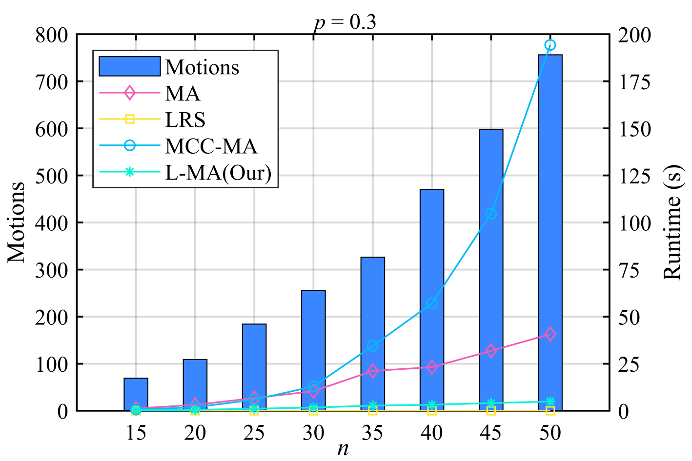
(a)

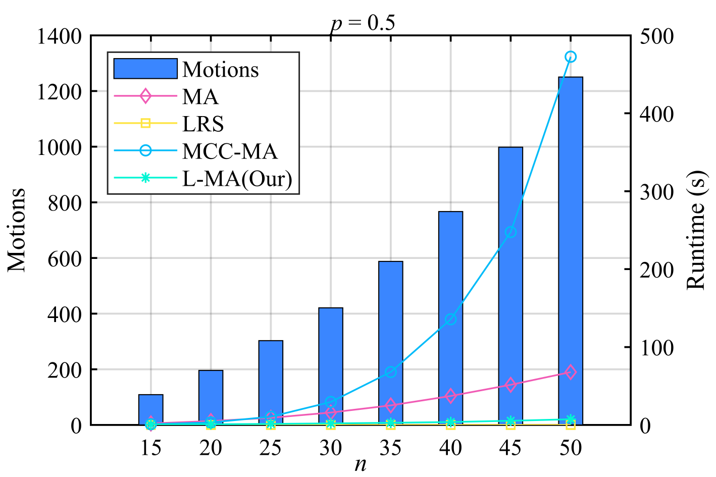
(b)

Figure 1: Runtimes of different methods (in seconds) and the numbers of relative motions. All results are plotted vs. $n$, with $p=0.3$ (left) and $p=0.5$ (right).

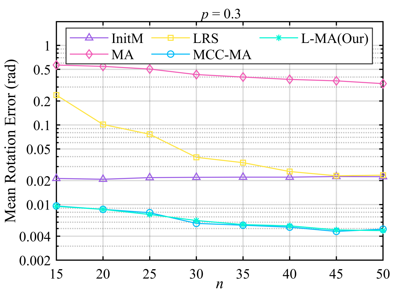
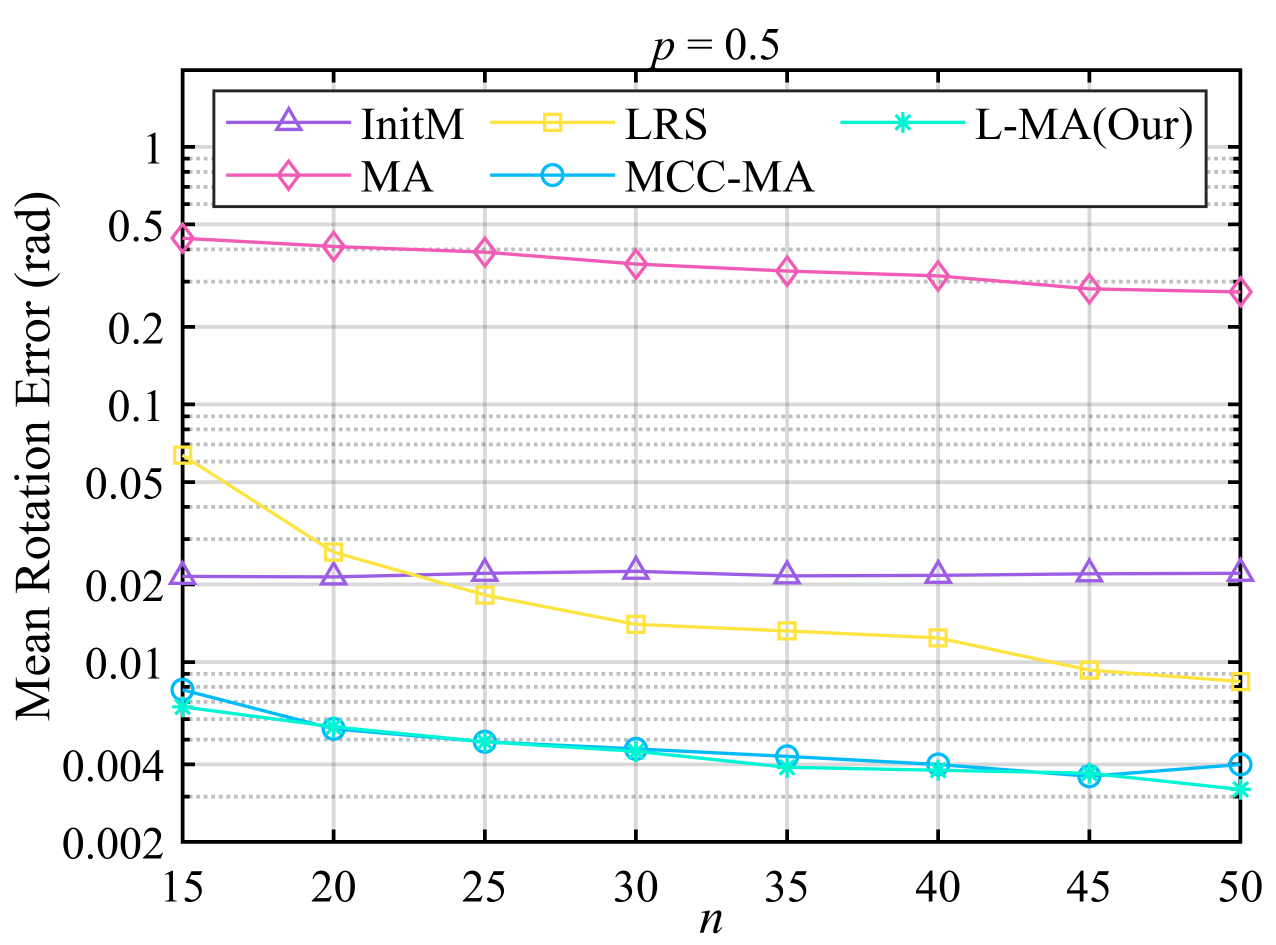
(a)

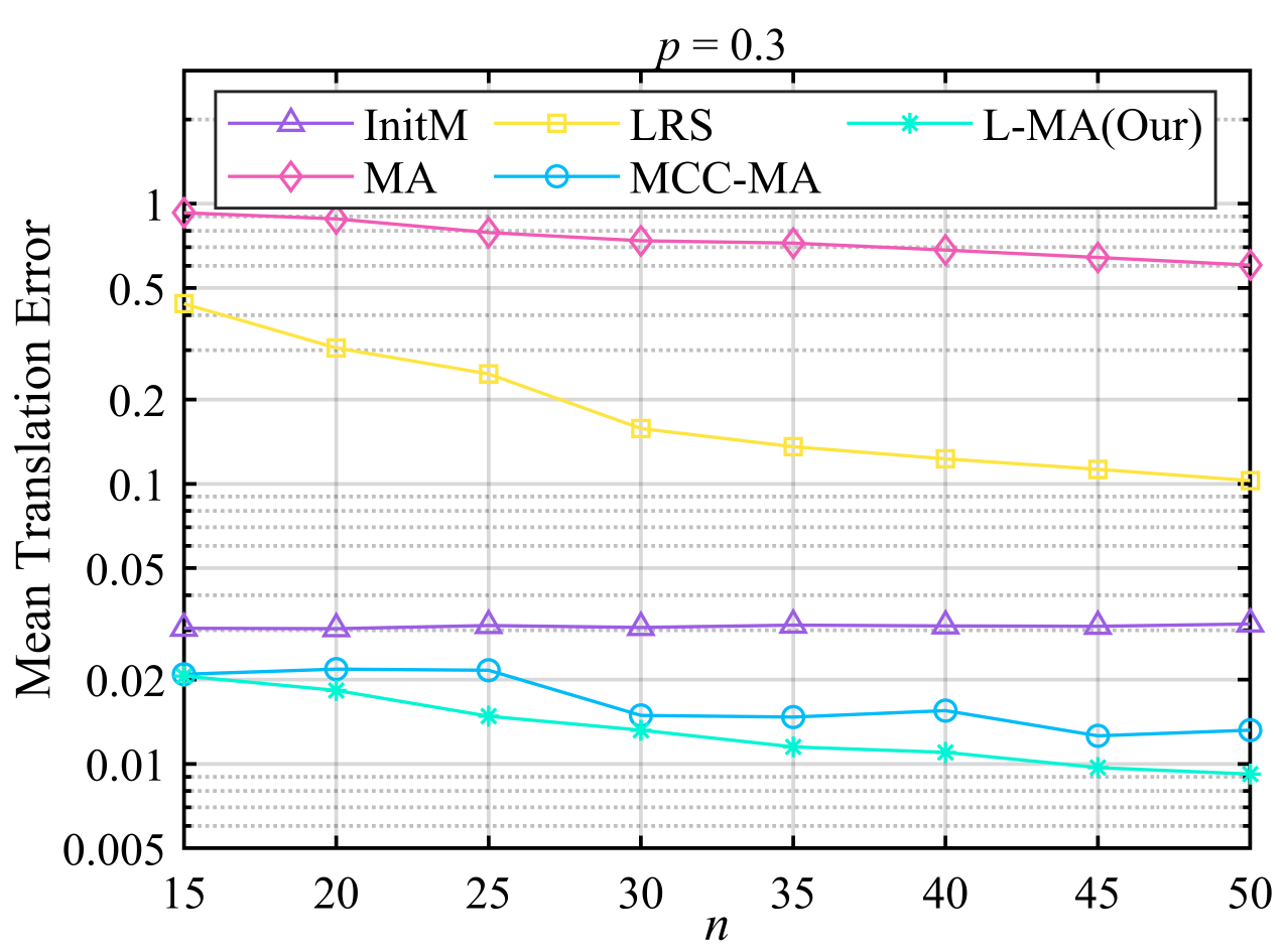
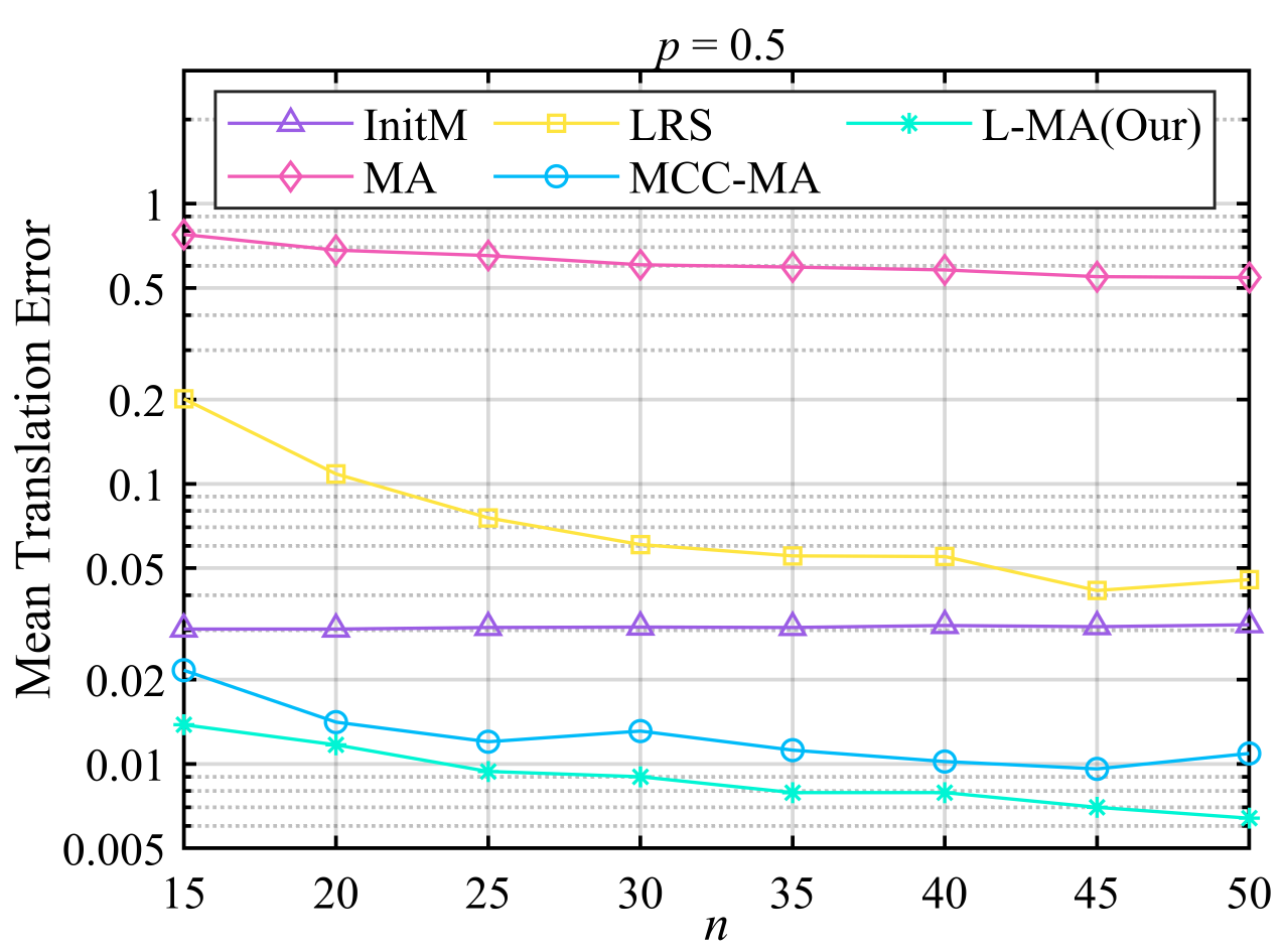
(b)

Figure 2: Performance comparison among different methods under different number of views $n$. The mean errors are plotted vs. $n$, with $p=0.3$ (top) and $p=0.5$ (bottom).

2). As all methods mentioned in this subsection require relative motions as input, we obtained the view-graph of relative motions by the Erdős-Rényi model with parameters $\left(n,p\right)$, where $p$ can be considered as the probability that there exists edge $\left(i,j\right)$ connecting node $i$ and $j$. Furthermore, for the studies of the robustness to noise and outliers of different methods, we generate the outliers from the original relative motions with parameter $q$ which denotes the probability that one edge is the outlier. For example, half of the relative motions are corrupted for the case in which $q=0.5$. The generation model of motions of these outliers is similar to that of global motions. Moreover, the motions of inliers are generated with parameters $\sigma_{\mathbf{R}}^{inlier}$ and $\sigma_{\mathbf{t}}^{inlier}$ which can be expressed as

$$\begin{cases}\mathbf{R}_{ij}^{inlier}=svd\left(\mathbf{R}_{ij}^{*}+\sigma_{\mathbf{R}}^{inlier}{{\boldsymbol{W}}_{\mathbf{R}}}\right)\\ \mathbf{t}_{ij}^{inlier}=\mathbf{t}_{ij}^{*}+\sigma_{\mathbf{t}}^{inlier}{\boldsymbol{W}_{\mathbf{t}}}\\ \end{cases}$$ (43)

where $\mathbf{R}_{ij}^{*}$ and $\mathbf{t}_{ij}^{*}$ denote, respectively, the rotation matrix and the translation vector of the relative motion $\mathbf{M}_{ij}^{*}={{\left(\mathbf{M}_{j}^{*}\right)}^{-1}}\mathbf{M}_{i}^{*}$; $\sigma_{\mathbf{R}}^{inlier}$, $\sigma_{\mathbf{t}}^{inlier}$ stand for the noise level of rotation and translation of inliers, respectively.

From the foregoing settings and definitions, the simulated model used in the experiment is affected by parameters $\left\{n,p,q,\sigma_{\mathbf{R}}^{init},\sigma_{\mathbf{t}}^{init},\sigma_{\mathbf{R}}^{inlier},\sigma_{\mathbf{t}}^{inlier}\right\}$. Obviously, several parameters do not allow us to take all the performance indices into account during the comparative experiment. Hence, similar to lots of works of literature, in the following experiments, we changed one part of the parameters, while the others remained fixed, to explore the influence of methods by different parameters, so as to evaluate the performances of methods. Additionally, in order to eliminate the randomness of simulation data, the results reported in the following subsections are the average values of 50 experiments with the same parameters, unless otherwise specified.

IV-A1 Efficiency and Accuracy

To validate the efficiency and accuracy of our method, we compared the different methods for a set of test parameters. In this experiment, we let $n$ vary between 15 and 55, in which case $p=0.3$ and $0.5$. More specifically, the larger $n$ and $p$, the greater the number of relative motions needed to be averaged. In both cases, $\sigma_{\mathbf{R}}^{inlier}=\sigma_{\mathbf{t}}^{inlier}=0.01$, $\sigma_{\mathbf{R}}^{init}=\sigma_{\mathbf{t}}^{init}=0.02$ and $q=0.3$. Under the condition that $p$ is fixed, apparently, the indices, such as computation time, and averaged error, can be considered as functions of $n$.

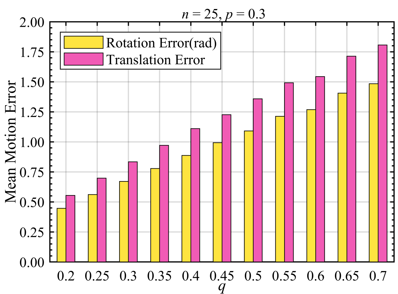
(a)

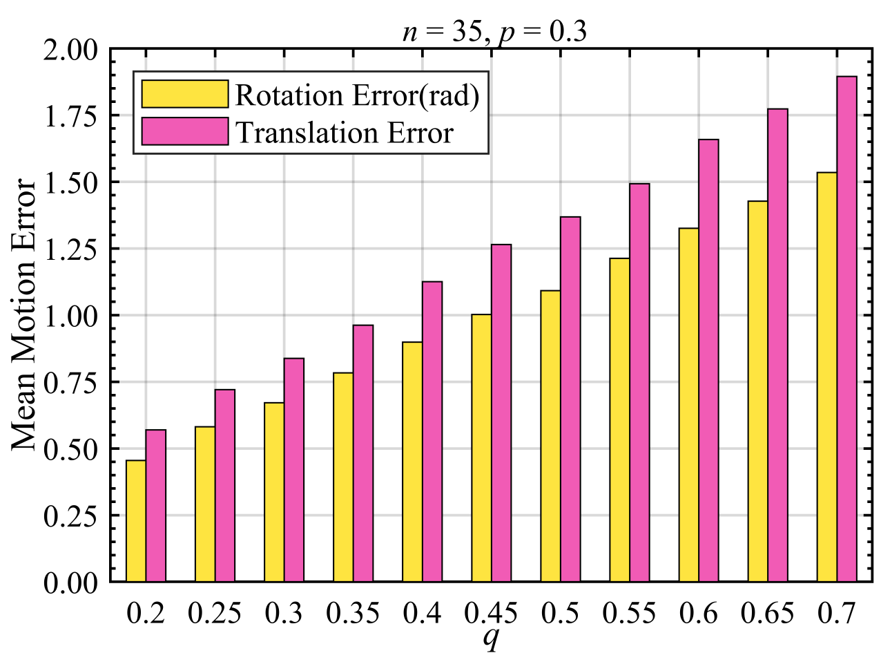
(b)

Figure 3: Mean motion error of relative motions under different outlier ratios. The mean rotation and translation errors are displayed vs. the outlier ratio $q$, with $n=25$ (left) and $n=35$ (right). Obviously, as we increase outlier ratio, the motion errors of relative motions increase almost linearly.

The averaging runtimes, and numbers of relative motions are depicted in Fig.1. The mean errors of rotation and translation of different methods are plotted in Fig.2. As illustrated in Fig.2, our method and MCC-MA achieve the lowest rotation error in all simulated data, and our method can always achieve the lowest translation error than the other methods. In addition, MA achieves the worst accuracy in both rotation and translation. Compared with MA, LRS obtains the more accurate results and achieves the third highest accuracy.

In detail, the performance of MA is more affected than other methods by outliers. Therefore, the accuracy of results achieved by MA is significantly reduced even when the set of relative motions only contains one outlier [14]. In addition, LRS is more sensitive to the sparsity of the view-graph than the other methods, this is the reason why there is a limit on the accuracy of LRS. Moreover, by virtue of the property of correntropy measure, our method and MCC-MA can assign different weight to each relative motion automatically so as to pay attention to the reliable relative motions and achieve more accurate results compared with MA and LRS.

Furthermore, we have also observed in Fig.1 and Fig.2 an interesting phenomenon: the mean errors of all methods decrease with the increase of the number of absolute motions $n$ or/and the value of $p$ when the other parameters are fixed. The reason for this phenomenon is that the increase of $n$ and/or $p$ will lead to the increase in the relevance of each node of the view-graph, that is, the increase in information redundancy, so that the errors of each absolute motion can be better averaged under the characteristics of the motion average algorithm. We would like to emphasize that the phenomenon only occurs in the simulation case where the outlier ratio and noise levels are fixed. In practice, the outlier ratio and noise levels of relative motions vary with the number of relative motions.

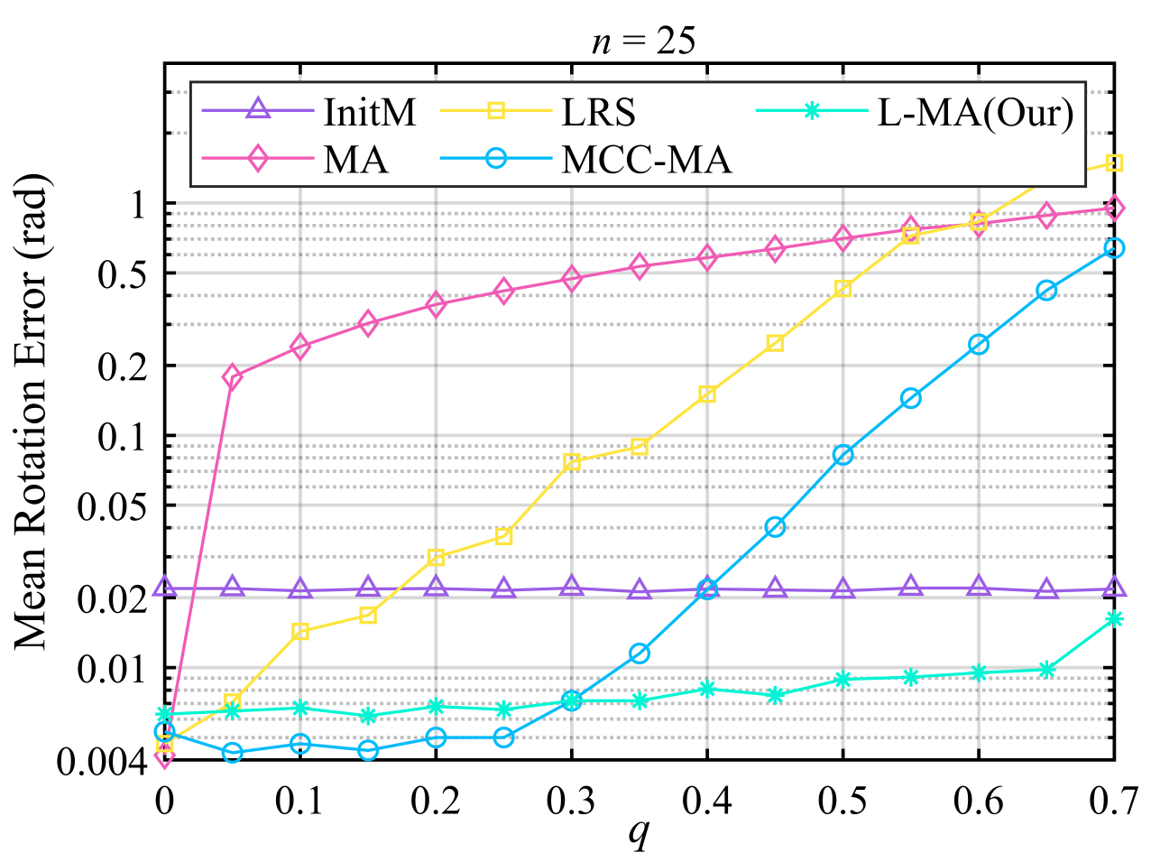
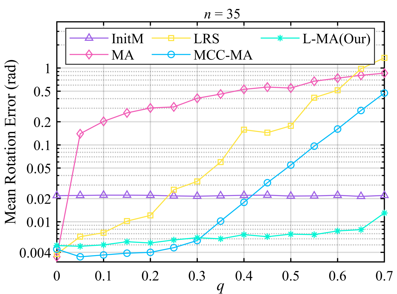
(a)

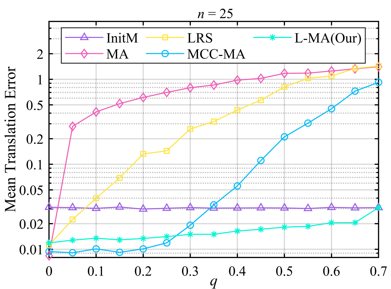
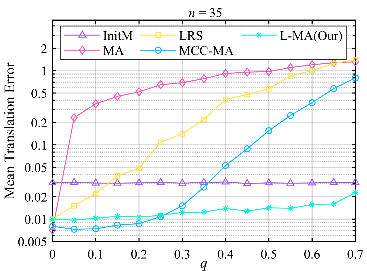
(b)

Figure 4: Mean motion error of relative motions under different outlier ratios. The mean rotation and translation errors are displayed vs. the outlier ratio $q$, with $n=25$ (left) and $n=35$ (right). Obviously, as we increase outlier ratio, the motion error of relative motions increases almost linearly.

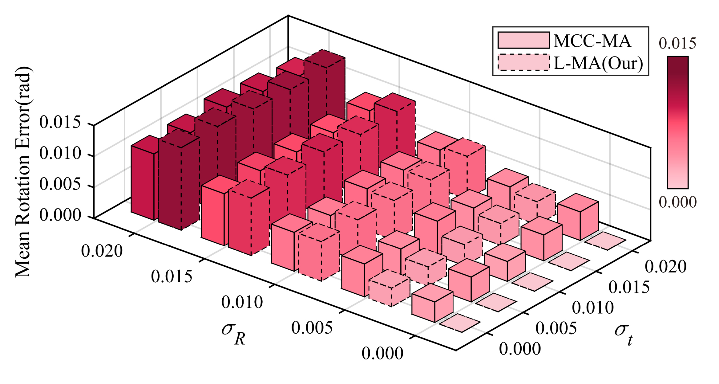
(a)

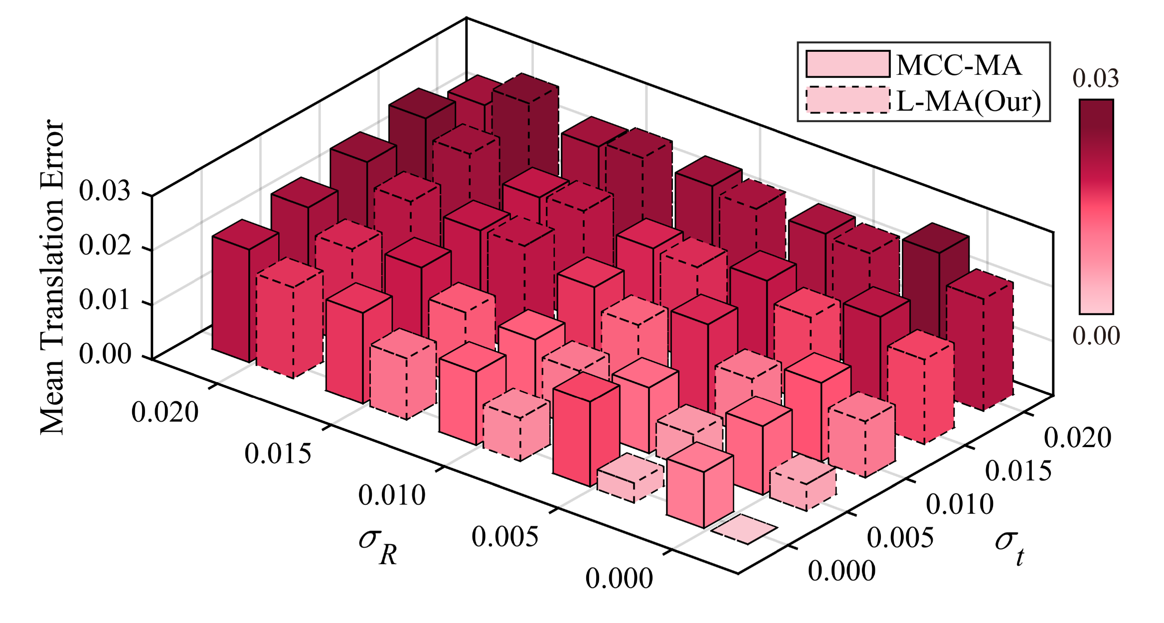
(b)

Figure 5: Performance comparison among MCC-MA and L-MA (Our) under different noise level of inliers. The mean rotation and translation errors are depicted vs. noise levels of rotation and translation $\sigma_{\mathbf{R}}^{inlier}$, $\sigma_{\mathbf{t}}^{inlier}$. In that figure, the results achieved by MCC-MA and our method are marked with full lines and dashed lines, respectively.

Moreover, as recorded in Fig.1, LRS is the most efficient method and our method has the second fastest speed. Besides, MCC-MA consumes more time than MA, this is because MCC-MA needs to update the weight matrix in each iteration. In addition, what we observe is that an increase in the number of relative motions leads to a significant increase in runtimes of MMA and MA and a slight increase in that of our method and LRS. For MCC-MA and MA, a fundamental step is to calculate the pseudo-inverse of a large matrix whose the size of columns is the linear function of the number of relative motions, which is very time-consuming. Apparently, for our method, the main computation in each iteration is to solve the SOCP problem, as given in (39). However, benefiting from the rapid convergence speed of SOCP, the number of iterations required by our method is far less than that of MCC-MA so our method is more efficient than MCC-MA and its runtime usually remains close to LRS. In short, Our method achieves the overall best performance, in terms of accuracy and efficiency.

IV-A2 Robustness to Outliers

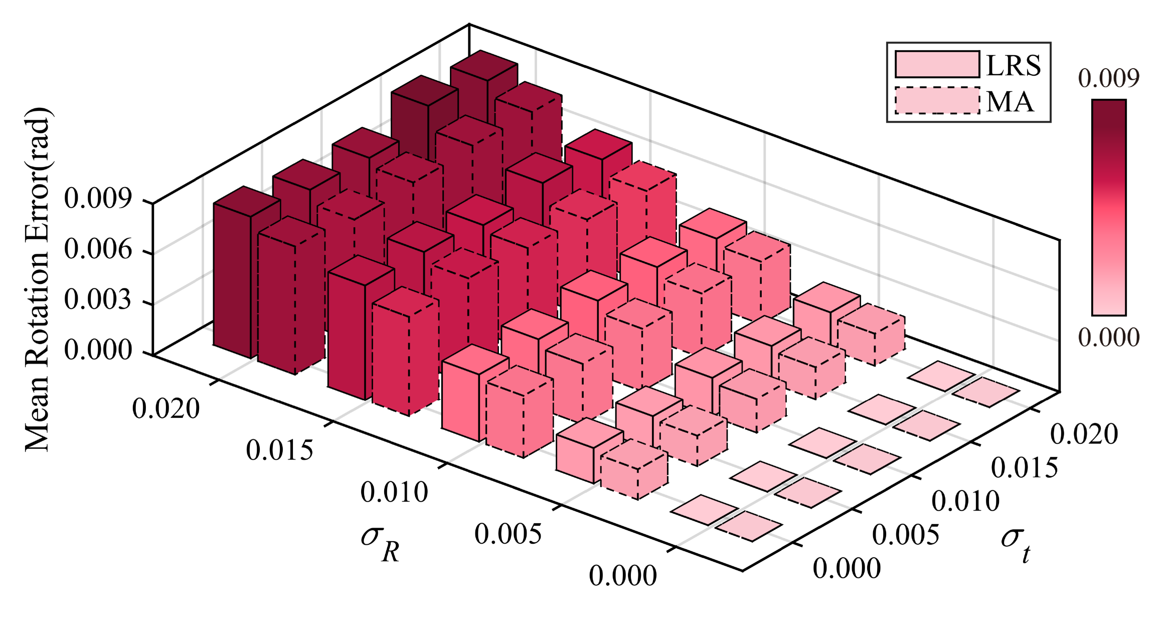
(a)

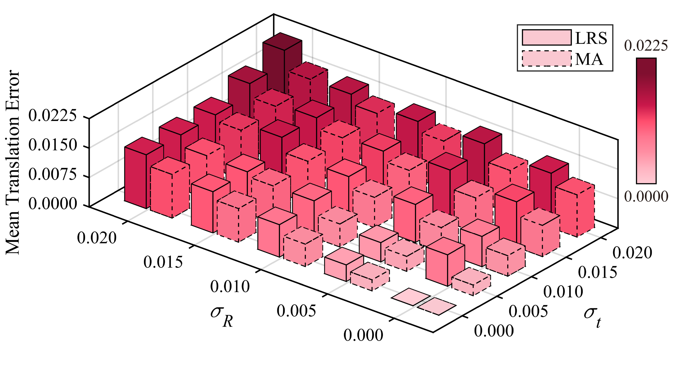
(b)

Figure 6: Performance comparison among LRS and MA under different noise levels of inliers. The mean rotation and translation errors are depicted vs. noise levels of rotation and translation $\sigma_{\mathbf{R}}^{inlier}$, $\sigma_{\mathbf{t}}^{inlier}$. In that figure, the results achieved by LRS and MA are marked with full lines and dashed lines, respectively.

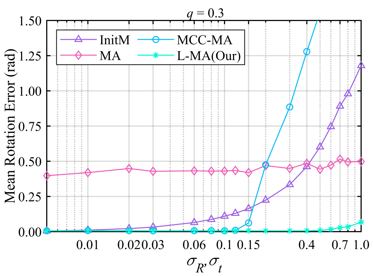
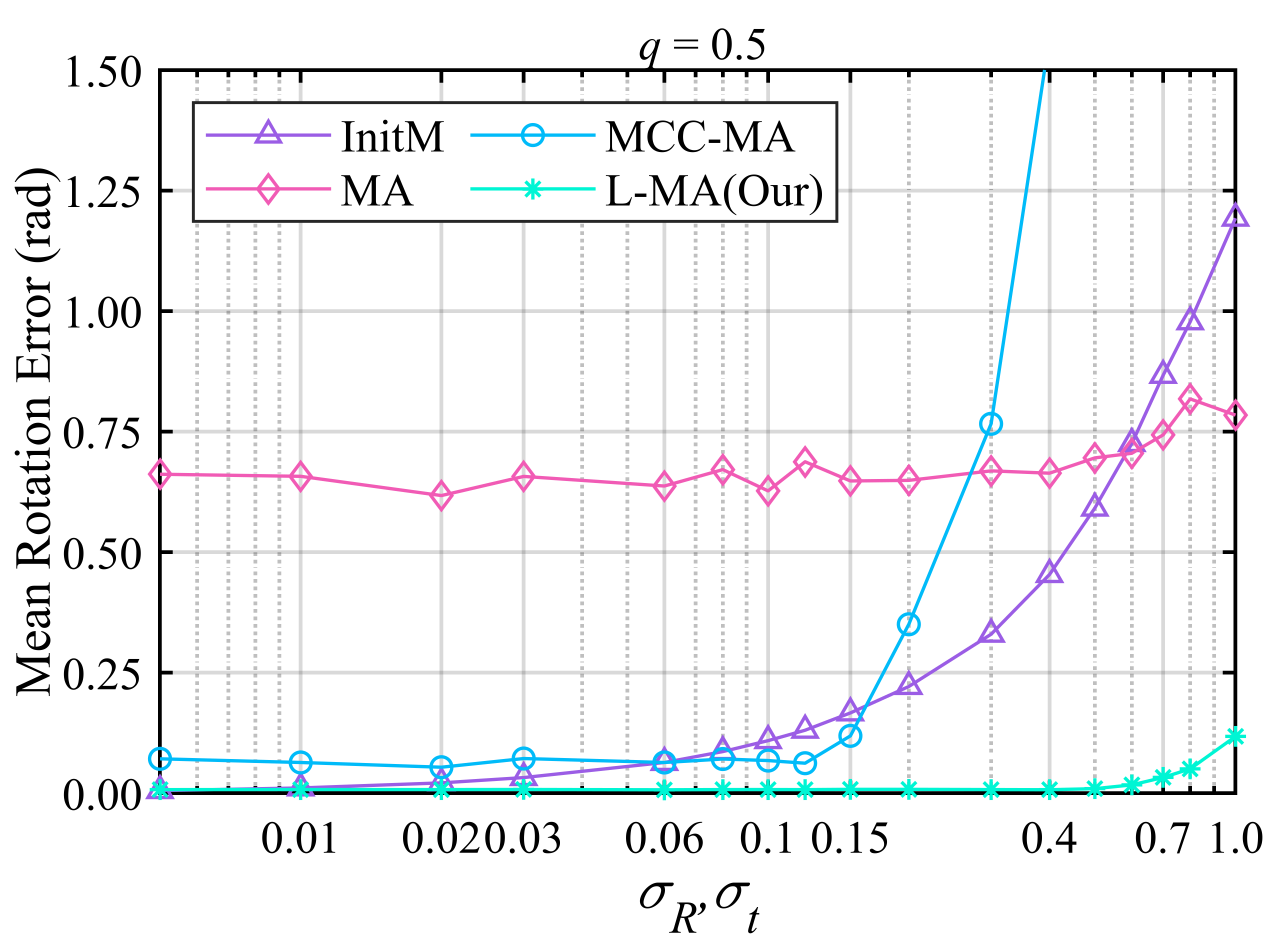
(a)

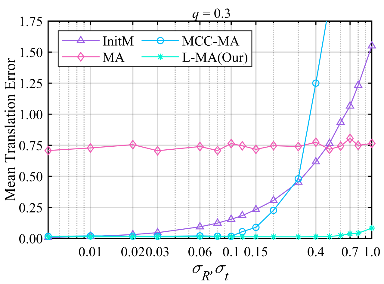
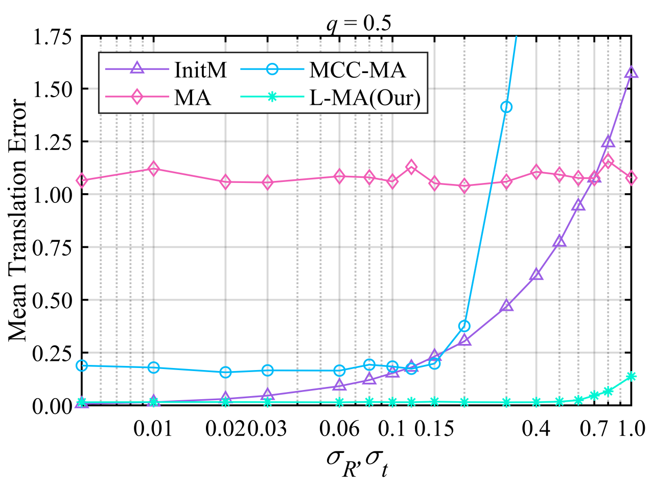
(b)

Figure 7: Performance comparison among different methods under different initial motions. All mean errors are plotted vs. noise levels of ground truth $\sigma_{\mathbf{R}}^{init}$, $\sigma_{\mathbf{t}}^{init}$, with $q=0.3$ (top) and $q=0.5$ (bottom). In this experiment, we apply different noises to ground truth so as to obtain different initial motions. For the sake of simplicity, the noise level of rotation is set equal to that of translation.

To study the robustness to outliers of different methods, a comparative experiment is carried out with different values of $q$. In this experiment, the value of $q$ varies between $0.0\sim 0.7$, indicating that the set of relative motions includes about $0\%\sim 70\%$ outliers. We considered two cases: $n=25$ and $n=35$. In both cases, $\sigma_{\mathbf{R}}^{inlier}=\sigma_{\mathbf{t}}^{inlier}=0.01$, $\sigma_{\mathbf{R}}^{init}=\sigma_{\mathbf{t}}^{init}=0.02$ and $p=0.3$.

We report the mean motion errors of relative motions as functions of $q$ in Fig.3. Moreover, we illustrate the results achieved by different methods in Fig.4. As depicted in Fig.3, with a increase in the value of $q$, the mean error of relative motions increases continuously. We have seen in Fig.4 that an increase in the outlier ratio leads to a decrease in the accuracy of all compared methods, the significant decrease in that of LRS and MCC-MA particularly. It should be noted, that our method can attain a relatively high accuracy for both rotation and translation even when $65\%$ of relative motions are outliers, demonstrating the strong robustness of our method to outliers. In addition, MA obtains, not surprisingly, the most accurate results when the outlier ratio is zero.

Moreover, as mentioned previously, the performances of our method and MCC-MA are affected by the kernel width. Instead of the mean of all Frobenius norms of residual error adopted in MCC-MA, we choose the median of residuals as kernel width as defined in (39), and hence, befitting from the characteristics of the median value, our method is more robust to outliers than MCC-MA. In addition, MCC-MA outperforms our method when the outlier ratio is small to $25\%$. This is because we set the value of the parameter $\alpha$, introduced in Section II.D, is $0.7$, indicating that the proposed method, to a certain extent, neglects the information supplied by the remaining $30\%$ relative motions which may lead to a slight loss of registration errors. Even so the accuracy of our method is still very close to that of MCC-MA under a low outlier ratio.

IV-A3 Effect of Noises

The performance of all compared methods is determined not only by the outlier ratio of relative motions, but also by the noise levels of inliers. Thus, in order to evaluate the effect of the latter, we carried out comparative experiments with different values of $\sigma_{\mathbf{R}}^{inlier}$, $\sigma_{\mathbf{t}}^{inlier}$. As both MA and LRS are poor in handling outliers, we set, respectively, the values of $q$ are $0$ for them and $0.3$ for MCC-MA and our method. In both experiments, we fixed the values of other parameters, i.e., $\sigma_{\mathbf{R}}^{inlier}=\sigma_{\mathbf{t}}^{inlier}=0.01$, $p=0.3$ and $n=30$.

Fig.5 illustrates the averaged results of MCC-MA and our method under different levels of noise and Fig.6 shows that of MA and LRS. As we saw in Fig.5 and Fig.6, with the increase in the noise level of inliers, the accuracies of all methods tested in this experiment rapidly decrease, indicating that the noise level of inliers has a very important influence on performances of all tested methods. Thus, we can draw the following conclusion: the reliability of the inliers is a critical prerequisite to obtaining excellent results for motion average algorithms. In addition, as displayed in Fig.5, compared to MCC-MA, our method is more sensitive to the noise level of inliers because (9) is satisfied as $\boldsymbol{\mathcal{J}}_{l}^{-1}\left(\boldsymbol{\xi}_{ij}^{k-1}\right)\approx\mathbf{I}$ and $\boldsymbol{\mathcal{J}}_{r}^{-1}\left(\boldsymbol{\xi}_{ij}^{k-1}\right)\approx\mathbf{I}$ if and only if the residual $\Delta\mathbf{M}_{ij}^{k-1}$ is “small”, i.e., if the noise levels of inliers are sufficiently close to zero. Fortunately, the pair-wise registration algorithms which have high registration accuracies, such as Robust ICP [25] , or Sparse ICP [26], may be used to avoid this drawback. In addition, a phenomenon that can be observed in both Fig.5 and Fig.6 is that, when the noise level of rotation remains constant, the increase in the noise level of translation does lead to the loss of rotational accuracy; in turn, the errors in both rotation and translation increase with noise level of rotation increasing when the noise level of translation remains constant.

IV-A4 Sensibility to the Initial Global Motions

As mentioned previously, the performances of MA, MCC-MA, and our method are dependent on the good initial motions. Thus, to study the sensibility to the initial global motion, experiments are carried out with different values of $\sigma_{\mathbf{R}}^{init}$, $\sigma_{\mathbf{t}}^{init}$. In both cases, $\sigma_{\mathbf{R}}^{inlier}=\sigma_{\mathbf{t}}^{init}=0.01$ and $n=30$. Specially, we tested the algorithms under different outlier ratios, i.e., $q=0.3$ and $q=0.5$. Fig.7 shows the mean errors of results obtained by different methods as a function of $\sigma_{\mathbf{R}}^{init}$, and of $\sigma_{\mathbf{t}}^{init}$.

As illustrated in Fig.7, MCC-MA is difficult to recover global motion when the noise level of initialization exceeds 0.15 and the performance of MCC-MA rapidly decreases as we continuously increase the noise level of initialization. On the on hand, the pseudo-inverse of $\boldsymbol{J}$ that MCC-MA needed to determine in each iteration may cause a convergence problem and further lead to a failure of multi-view registration because it is easy to be singular under poor initializations. On the other hand, poor initializations may lead to the kernel width for MCC-MA in the first iteration so large as to assign unreliable weight for each relative motion. Compared to MCC-MA, our method always converges to good global motions, even though the noise level of initialization is $0.4$. What this implies is that our method has the low sensibility to the initialization and a large convergence domain.

IV-B Real Data

TABLE I: Statistics Information of Relative Motions under
$30\%$ Overlap Percentage Threshold

Dataset	Motions	Rotation error(rad)		Translation error(mm)
		Mean	Meadian	Mean	Meadian
Armadillo	57	0.0478	0.0042	5.5610	0.3409
Buddha	96	0.2200	0.0043	2.1814	0.4097
Bunny	45	0.0789	0.0025	3.0070	0.2889
Dragon	77	0.2786	0.0041	20.839	0.3641

TABLE II: Statistics Information of Relative Motions under
$20\%$ Overlap Percentage Threshold

Dataset	Motions	Rotation error(rad)		Translation error(mm)
		Mean	Meadian	Mean	Meadian
Armadillo	81	0.3724	0.0057	15.015	0.4907
Buddha	131	0.6428	0.0059	5.6311	0.5352
Bunny	64	0.5363	0.0045	28.069	0.4160
Dragon	115	0.7042	0.0080	53.874	0.5778

TABLE III: Performance Comparison among Different Multi-view Registration Methods
on Four Data Sets under $30\%$ Overlap Percentage Threshold

Methods	Armadillo				Buddha				Bunny				Dragon
	${{e}_{\mathbf{R}}}$(rad)	${{e}_{\mathbf{t}}}$mm	T(s)	Iter	${{e}_{\mathbf{R}}}$(rad)	${{e}_{\mathbf{t}}}$mm	T(s)	Iter	${{e}_{\mathbf{R}}}$(rad)	${{e}_{\mathbf{t}}}$mm	T(s)	Iter	${{e}_{\mathbf{R}}}$(rad)	${{e}_{\mathbf{t}}}$mm	T(s)	Iter
InitM	0.0269	2.5680	$/$	$/$	0.0207	1.3401	$/$	$/$	0.0255	3.4404	$/$	$/$	0.0241	5.8683	$/$	$/$
LRS	0.0077	1.1133	$\mathbf{0.0091}$	$/$	0.0117	0.6307	$\mathbf{0.0171}$	$/$	0.0375	7.8921	$\mathbf{0.0133}$	$/$	0.6280	10.6777	$\mathbf{0.0169}$	$/$
MA	0.0854	12.5369	0.3685	66	0.1592	1.3574	1.0950	110	0.2232	13.4495	0.3522	78	0.4893	51.2763	1.1821	130
WMAA	0.0097	1.5094	0.3273	66	0.0191	0.6612	0.7586	83	0.0334	2.3219	0.2489	59	0.2475	28.5714	0.9293	120
MCC-MA	$\mathbf{0.0053}$	0.7094	0.3566	52	0.0084	0.6484	0.7879	62	0.0041	0.3480	0.2807	51	0.0121	0.9734	0.8759	87
L-MA(Our)	0.0072	$\mathbf{0.6838}$	0.2077	$\mathbf{8}$	$\mathbf{0.0062}$	$\mathbf{0.5659}$	0.2605	$\mathbf{7}$	$\mathbf{0.0027}$	$\mathbf{0.2308}$	0.1486	$\mathbf{6}$	$\mathbf{0.0089}$	$\mathbf{0.7571}$	0.3889	$\mathbf{12}$

(a)

(b)

(c)

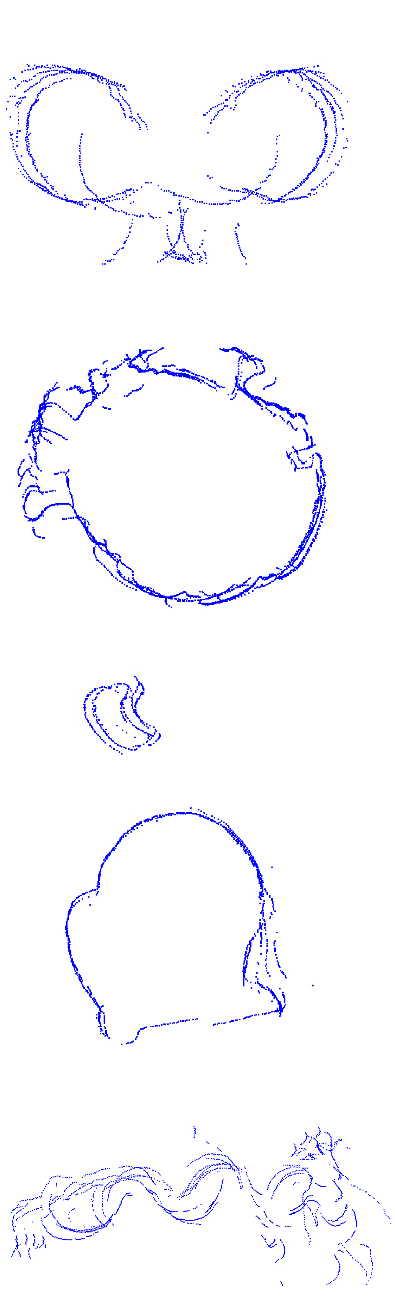
(d)

(d)

(e)

(f)

(g)

Figure 8: Multi-view registration results of different methods presented in the form of cross-section for four data sets under $30\%$ overlap percentage threshold: (a) Ground truth models. (b) Initial results. (c) LRS results. (d) MA results. (e) WMAA results. (f) MCC-MA results. (g) Our results.

In this experiment, we compare the performance of different methods on four benchmark data sets, which are taken from the Stanford 3D Scanning Repository [30] (Bunny, Buddha, Dragon, and Armadillo, which include $10$, $15$, $15$, and $12$ scans, respectively). For these data sets, the ground truths of global motions are available. Note that ground truths are only used for the evaluation of registration results and the input relative motions. To demonstrate the performance, our method is compared with four methods for motion averaging, including LRS, MA, MCC-MA, and WMAA. Since all compare methods take relative motions as input and the pair-wise registration algorithms are sensitive to partial overlaps, we adopted the method proposed in [16] to roughly estimate the overlapping percentage for each scan pair, and then utilize the pair-wise registration algorithm introduced in [7] to obtain relative motions for these scans pairs whose overlapping percentage are large than a pre-set threshold $\gamma_{thr}$. Moreover, we utilized feature-based registration [31] to estimate initial global motions for multi-view registration. To illustrate the performance of our method, we test the algorithms with different overlapping percentages, namely, $\gamma_{thr}=0.3$ and $\gamma_{thr}=0.2$. We evaluate the mean, and median error of the corresponding relative motions under these overlapping percentages.

The errors as well as the number of relative motions for $\gamma_{thr}=0.3$ and $\gamma_{thr}=0.2$, are summarized in Table I and Table II, respectively. Table III and Table IV record the registration results achieved by different methods. The column ’Iter’ indicates the number of iterations required by different methods for convergence and we did not report that of LRS because it is not an iterative algorithm. To visualize the registration results, we further provide the results of different methods presented in the form of cross-sections for $\gamma_{thr}=0.3$ and $\gamma_{thr}=0.2$ in Fig.8 and Fig.9, respectively.

As shown in Table I and Table II, relative motions contain many outliers and the outlier ratios increase with the decrease of the overlapping percentage threshold. Furthermore, as illustrated in Table III and Table IV, our method achieves the lowest mean rotation and translation on these data sets with different overlapping percentages, while MCC-MA only outperforms our method for the rotation estimation on Armadillo ($30\%$ threshold). As discussed in Subsection IV.A(1), LRS is the most efficient method but it fails to return accurate estimates of global motions for these relative motions whose outlier ratios are relatively high, such as Dragon, and Buddha. In addition, as reported on Table III and Table IV, the number of iterations of our method is nearly 10 times less than that of MA, WMAA, and MCC-MA because of the high convergence speed of our method. For this reason, our method is more efficient than MA, WMAA, and MCC-MA.

TABLE IV: Performance Comparison among Different Multi-view Registration Methods
on Four Data Sets under $20\%$ Overlap Percentage Threshold

Methods	Armadillo				Buddha				Bunny				Dragon
	${{e}_{\mathbf{R}}}$(rad)	${{e}_{\mathbf{t}}}$mm	T(s)	Iter	${{e}_{\mathbf{R}}}$(rad)	${{e}_{\mathbf{t}}}$mm	T(s)	Iter	${{e}_{\mathbf{R}}}$(rad)	${{e}_{\mathbf{t}}}$mm	T(s)	Iter	${{e}_{\mathbf{R}}}$(rad)	${{e}_{\mathbf{t}}}$mm	T(s)	Iter
InitM	0.0269	2.5680	$/$	$/$	0.0207	1.3401	$/$	$/$	0.0255	3.4404	$/$	$/$	0.0241	5.8683	$/$	$/$
LRS	0.0318	2.9198	$\mathbf{0.0114}$	$/$	1.5279	7.9560	$\mathbf{0.0192}$	$/$	0.0834	8.2177	$\mathbf{0.0147}$	$/$	0.3576	21.8699	$\mathbf{0.0188}$	$/$
MA	0.2679	24.6564	0.7799	79	0.1259	2.7785	1.7219	109	0.4636	39.7073	0.7098	81	0.5851	54.4524	2.2276	142
WMAA	0.0286	2.1120	0.5061	61	0.0242	0.7471	1.2842	86	0.0488	4.0199	0.3246	48	0.2992	33.2293	1.6596	126
MCC-MA	0.0211	0.9076	0.7553	67	0.0797	0.7101	2.0911	101	0.0080	0.6721	0.4441	50	0.0387	1.3876	1.5368	90
L-MA(Our)	$\mathbf{0.0055}$	$\mathbf{0.6947}$	0.1653	$\mathbf{5}$	$\mathbf{0.0058}$	$\mathbf{0.5668}$	0.3622	$\mathbf{8}$	$\mathbf{0.0019}$	$\mathbf{0.2508}$	0.1748	$\mathbf{6}$	$\mathbf{0.0091}$	$\mathbf{0.7422}$	0.4552	$\mathbf{12}$

(a)

(b)

(c)

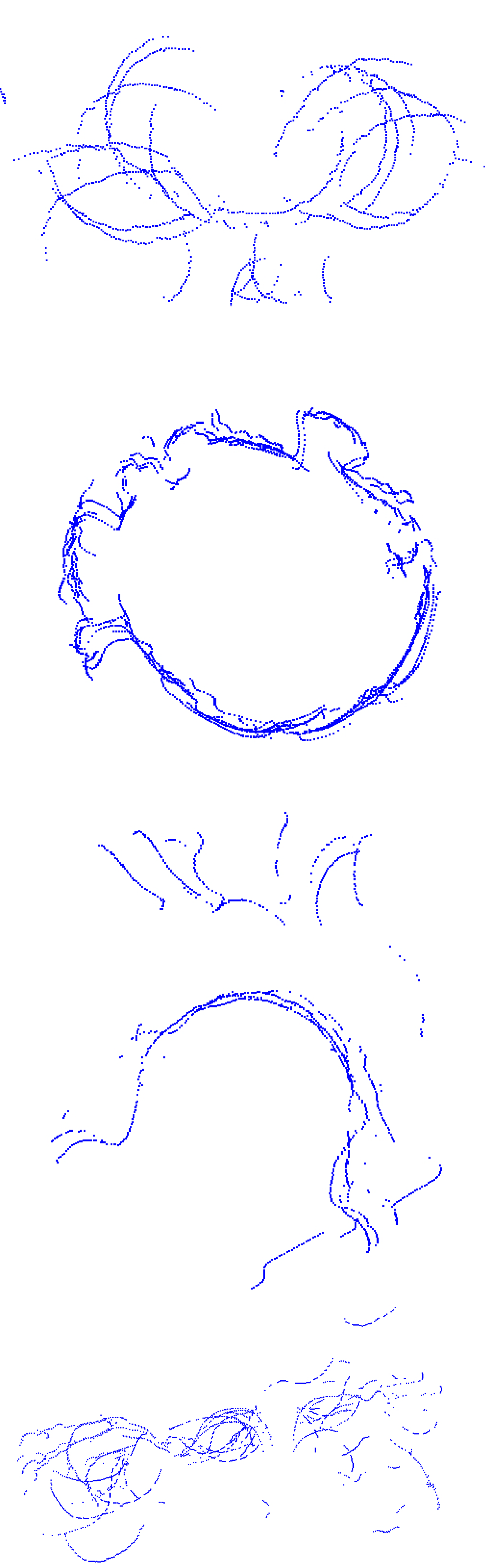
(d)

(d)

(e)

(f)

(g)

Figure 9: Multi-view registration results of different methods presented in the form of cross-section for four data sets under $20\%$ overlap percentage threshold: (a) Ground truth models. (b) Initial results. (c) LRS results. (d) MA results. (e) WMAA results. (f) MCC-MA results. (g) Our results.

Furthermore, we can see that our performance under $20\%$ overlapping percentage even outperforms the performance under $30\%$ overlapping percentage. The fact can be easily interpreted by virtue of the conclusions drawn in Subsection IV.A(1) and IV.A(2): the decrease of overlapping percentage leads to the increase of the relevance of each scan, but also the increase of outliers; as we saw in Subsection IV.A(1) and IV.A(2), the former will lead to an increase of accuracies of all methods, while the latter will cause only a slight decrease the accuracy of our method, but a rapid decrease of those of others methods. This also reveals the reason why the registration results achieved by WMAA are not promising, that is, high overlap does not imply a high accuracy of pair-wise registration results. In short, one advantage of our method lies in the fact that it can efficiently and accurately exploit the redundancy information in the set of relative motions, even though the outlier ratio of the set is relatively high.

V Conclusion and Future Work

In conclusion, we proposed a novel motion averaging framework with Laplacian kernel-based maximum correntropy criterion. In particular, we adopted an iterative strategy for determining the global motions similar to many works in previous literature. The task at hand, namely, finding the increment of global motions, can then be formulated as an optimization problem aimed at maximizing an objective function by virtue of LMCC. Furthermore, the optimization problem can be divided into subproblems: obtain the weights according to current residuals and solve a SOCP problem based on the weights, so that our method can efficiently avoid the computation of the inverse of a large matrix occurring in many works of literature. We also introduced a new method to determine kernel width. Experimental tests on synthetic and data sets demonstrate that our method has state-of-the-art multi-view registration accuracy, high robustness to outliers, and low sensibility to initial global motions.

References

- [1] D. Zhen et al., “Registration of large-scale terrestrial laser scanner point clouds: A review and benchmark,” ISPRS J. Photogramm. Remote Sens., vol. 163, pp. 327-342, Apr. 2020.
- [2] J. Li, Q. Hu, Y. Zhang, and M. Ai, “Robust symmetric iterative closest point,” ISPRS J. Photogramm. Remote Sens., vol. 185, pp. 219-231, Mar. 2022.
- [3] P. J. Besl and N. D. McKay,“A method for registration of 3-D shapes,” IEEE Trans. Pattern Anal. Mach. Intell., vol. 14, no. 2, pp. 239-256, Feb. 1992.
- [4] J. Yang, H. Li, D. Campbell, and Y. Jia, “Go-ICP: A globally optimal solution to 3D ICP point-set registration,” IEEE Trans. Pattern Anal. Mach. Intell., vol. 38, no. 11, pp. 2241-2254, Feb. 1992.
- [5] Y. Chen and G. Medioni, “Object modelling by registration of multiple range images,” Image Vis. Comput., vol. 10, no. 3, pp. 145-155, Apr. 1992.
- [6] A. Segal, D. Haehnel, and S. Thrun, “Generalized-icp,” in Robot. Sci., Syst., vol. 2, no. 4, pp. 435, Jun. 2009.
- [7] S. Rusinkiewicz, “A symmetric objective function for ICP,” ACM Trans. Graphics, vol. 38, no. 4, pp. 1-7, Aug. 2019.
- [8] J. Zhu, J. Hu, H. Lu, B. Chen, Z. Li, and Y Li, “Robust motion averaging under maximum correntropy criterion,” in Proc. IEEE Int. Conf. Robot. Autom. (ICRA), May. 2021, pp. 5283-5288.
- [9] Y. Chen and G. Medioni, “Object modelling by registration of multiple range images,” Imag. Vis. Comput., vol. 10, no. 3, pp. 145-155, Apr. 1992.
- [10] T. Weber, R. Hänsch, and O. Hellwich, “Automatic registration of unordered point clouds acquired by Kinect sensors using an overlap heuristic,” ISPRS J. Photogramm. Remote Sens., vol. 102, pp. 96-109, Apr. 2015.
- [11] J. B. Kruskal, “On the shortest spanning subtree of a graph and the traveling salesman problem,” Proc. Am. Math. Soc., vol. 7, no. 1, pp. 48-50, Feb. 1956.
- [12] J. Zhu, L. Zhu, Z. Li, C. Li, and J. Cui, “Automatic multi-view registration of unordered range scans without feature extraction,” Neurocomputing, vol. 171, pp. 1444-1453, Jan. 2016.
- [13] G. D. Evangelidis and R. Horaud., “Joint alignment of multiple point sets with batch and incremental expectation-maximization,” IEEE Trans. Pattern Anal. Mach. Intell., vol. 40, no. 6, pp. 1397-1410, Jun. 2017.
- [14] J. Zhu, R. Guo, Z. Li, J. Zhang, and S. Pang, “Registration of multi-view point sets under the perspective of expectation-maximization,” IEEE Trans. Image Process., vol. 29, pp. 9176-9189, Sep. 2020.
- [15] V. M. Govindu and A. Pooja, “On averaging multiview relations for 3D scan registration,” IEEE Trans. Image Process., vol. 23, no. 3, pp. 1289-1302, Feb. 2013.
- [16] Z. Li, J. Zhu, K. Lan, C. Li, and C. Fang, “Improved techniques for multi-view registration with motion averaging,” in Proc. Int. Conf. 3D Vis. (3DV), Dec. 2014, pp. 713-719.
- [17] R. Guo, J. Zhu, Y. Li, D. Chen, Z. Li, and Y. Zhang, “Weighted motion averaging for the registration of multi-view range scans,” Multimed. Tools. Appl., vol. 77, no. 9, pp. 10651-10668, Apr. 2018.
- [18] V. M. Govindu, “Robustness in motion averaging,” in Asian Conf. Comput. Vis. (ACCV), Jan. 2006, pp. 457-466.
- [19] F. Arrigoni, B. Rossi, and A. Fusiello, “Global registration of 3d point sets via lrs decomposition,” in Eur. Conf. Comput. Vis. (ECCV), Oct. 2016, pp. 489-504.
- [20] F. Arrigoni, B. Rossi, P. Fragneto, and A. Fusiello, “Robust synchronization in SO (3) and SE (3) via low-rank and sparse matrix decomposition,” Comput. Vis. Image Understand., vol. 174, pp. 95-113, Sep. 2018.
- [21] W. Liu, P. P. Pokharel, and J. C. Principe, “Correntropy: Properties and applications in non-Gaussian signal processing,” IEEE Trans. Signal Process., vol. 55, no. 11, pp. 5286-5298, Nov. 2007.
- [22] A. Singh, R. Pokharel, and J. Principe, “The C-loss function for pattern classification,” Pattern Recognit., vol. 47, no. 1, pp. 441-453, Jan. 2014.
- [23] R. He, W. Zheng, and B. Hu, “Maximum correntropy criterion for robust face recognition,” IEEE Trans. Pattern Anal. Mach. Intell., vol. 33, no. 8, pp. 1561-1576, Dec. 2010.
- [24] C. Hu, G. Wang, K. C. Ho, and J. Liang, “Robust ellipse fitting with Laplacian kernel based maximum correntropy criterion,” IEEE Trans. Image Process., vol. 30, pp. 3127-3141, Feb. 2021.
- [25] J. Zhang, Y. Yao, and B. Deng, “Fast and robust iterative closest point,” IEEE Trans. Pattern Anal. Mach. Intell., vol. 44, no. 7, pp. 3450-3466, Jan. 2021.
- [26] S. Bouaziz, A. Tagliasacchi, and M. Pauly, “Sparse iterative closest point,” in Comput. Graph Forum, vol. 32, no. 5, pp. 113-123, Aug. 2013.
- [27] J. Sola, J. Deray, and D. Atchuthan, “A micro Lie theory for state estimation in robotics,” arXiv preprint arXiv:1812.01537, 2018.
- [28] T. D. Barfoot., “State Estimation for Robotics: Matrix Lie Groups,” Cambridge, U.K.: Cambridge Univ. Press, 2015.
- [29] F. J. Sturm, “Using SeDuMi 1.02, a MATLAB toolbox for optimization over symmetric cones,” Optim. Methods Softw., vol. 11, nos. 1-4, pp. 625-653, Jan. 1999.
- [30] B. C. M. Levoy, J. Gerth, and K. Pull. (2005). The Stanford 3D Scanning Repository. [Online]. Available: http://www-graphics.stanford.edu/data/3dscanrep
- [31] H. Lei, G. Jiang, and L. Quan, “Fast descriptors and correspondence propagation for robust global point cloud registration,” IEEE Trans. Image Process., vol. 26, no. 8, pp. 3614-3623, May. 2017.