Higher-order adaptive methods for exit times of Itô diffusions

Abstract.

We construct a higher-order adaptive method for strong approximations of exit times of Itô stochastic differential equations (SDE). The method employs a strong Itô–Taylor scheme for simulating SDE paths, and adaptively decreases the step size in the numerical integration as the solution approaches the boundary of the domain. These techniques turn out to complement each other nicely: adaptive time-stepping improves the accuracy of the exit time by reducing the magnitude of the overshoot of the numerical solution when it exits the domain, and higher-order schemes improve the approximation of the state of the diffusion process.

We present two versions of the higher-order adaptive method. The first one uses the Milstein scheme as numerical integrator and two step sizes for adaptive time-stepping: $h$ when far away from the boundary and $h^{2}$ when close to the boundary. The second method is an extension of the first one using the strong Itô–Taylor scheme of order 1.5 as numerical integrator and three step sizes for adaptive time-stepping. For any $\xi>0$, we prove that the strong error is $\mathcal{O}(h^{1-\xi})$ and $\mathcal{O}(h^{3/2-\xi})$ for the first and second method, respectively, and the expected computational cost for both methods is $\mathcal{O}(h^{-1}\log(h^{-1}))$. Theoretical results are supported by numerical examples, and we discuss the potential for extensions that improve the strong convergence rate even further.

1. Introduction

For a bounded non-empty domain $D\subset\mathbb{R}^{d}$ and a $d-$dimensional Itô diffusion $(X_{t})_{t\geq 0}$ with $X(0)\in D$, the goal of this work is to construct efficient higher-order adaptive numerical methods for strong approximations of the exit time

$$\tau:=\inf\{t\geq 0\mid X(t)\notin D\}\wedge T,$$ (1)

where $T>0$ is given. The dynamics of the diffusion process is governed by the autonomous Itô stochastic differential equation (SDE)

$$\begin{split}\mathrm{d}X&=a(X)\mathrm{d}t+b(X)\mathrm{d}W\\ X(0)&=x_{0},\end{split}$$ (2)

where $a\colon\mathbb{R}^{d}\to\mathbb{R}^{d}$ and $b\colon\mathbb{R}^{d}\to\mathbb{R}^{d\times m}$, $x_{0}$ is a deterministic point in $D$, and $W$ is an $m$-dimensional standard Wiener process on a filtered probability space $(\Omega,\mathcal{F},(\mathcal{F}_{t})_{t\geq 0},\mathbb{P})$. Further details on the regularity of the domain $D$ and the coefficients of the SDE are provided in Section 2.

Our method employs a strong Itô–Taylor scheme for simulating SDE paths and carefully decreases the step size in the numerical integration as the solution approaches the boundary of the domain. We present two versions: the order 1 method and the order 1.5 method. The order 1 method uses the Milstein scheme as numerical integrator and two step sizes for the adaptive time-stepping depending on the proximity of the state the boundary of $D$: a larger time-step when far away and a smaller time-step when close to $\partial D$. The order 1.5 method uses the strong Itô–Taylor scheme of order 1.5 as numerical integrator and, as an extension of the previous method, three different step sizes for the adaptive time-stepping. When adaptive time-stepping is properly balanced against the order of the scheme the following results hold for any $\xi>0$: the order 1 method achieves the strong convergence rate $\mathcal{O}(h^{1-\xi})$, cf. Theorem 2.7; and the order 1.5 method achieves the strong convergence rate $\mathcal{O}(h^{3/2-\xi})$, cf.  Theorem 2.10. Theorems 2.8 and 2.11 further show that both of the higher-order adaptive methods have an expected computational cost of $\mathcal{O}(h^{-1}\log(h^{-1}))$.

Exit times describe critical times in controlled dynamical systems, and they have applications in pricing of barrier options [1] and also in American options [4], as the latter may be formulated as a control problem where exit times determine when to execute the option. They also appear in physics, for instance when studying the transition time between pesudo-stable states of molecular systems in the canonical ensemble [37].

The mean exit time problem may be solved by the Monte Carlo approach of direct simulation of SDE paths or by solving the associated partial differential equation; the Feynman–Kac equation [11]. In high-dimensional state space, the former approach is more tractable than the latter, due to the curse of dimensionality. A Monte Carlo method using the Euler–Maruyama scheme with a uniform timestep to simulated SDE paths was shown to produce the weak convergence rate 1/2 for approximating the mean exit time in [16]. An improved weak order 1 method was achieved by reducing the overshoot error through careful shifting of the boundary, cf. [6, 17, 18]. The weak order 1 method was extended to problems with time-dependent boundaries in [19], and [5] showed that in $L^{1}(\Omega)$-norm, the Euler–Maruyama scheme has order 1/2 convergence rate. The contributions of this work may be viewed as extensions of this strong convergence study to higher-order Itô–Taylor schemes with adaptive time-stepping.

Multilevel Monte Carlo (MLMC) methods for mean exit times have been developed in [20, 14]. Using the Euler–Maruyama scheme with boundary shifting and conditional sampling of paths near the boundary, the method [14] can reach the mean-square approximation error $\mathcal{O}(\epsilon^{2})$ at the near-optimal computational cost $\mathcal{O}(\epsilon^{-2}\log(\epsilon)^{2})$. Since our methods efficiently approximate the strong exit time and admit a pairwise coupling of simulations on different resolutions, they are also suitable for MLMC. See Section 5, for an outline of the extension to MLMC.

Adaptive methods for SDE with discontinuous drift coefficients have been considered in [34, 38]. Therein, the discontinuity regions of the drift coefficient are associated to hypersurfaces, and when one is close to such hypersurfaces, a small time-step is used, and otherwise a large time-step is used. This adaptive-time-stepping approach is similar to ours, as can be seen by viewing the boundary of $D$ in our problem as a hypersurface, but the problem formulations differ, and our method is more general in the sense that it admits a sequence of time-step sizes and also higher-order numerical integrators. For numerical testing of strong convergence rates, we have employed the idea of pairwise coupling of non-nested adaptive simulations of SDE developed in [15], which is an approach that also could be useful for combining our method with MLMC in the future. See also [29] for a recent contribution on a posteriori adaptive methods for weak approximations of exit times and states of SDE, and  [23, 9, 24] for other partly state-dependent adaptive MLMC methods for weak approximations of SDE in finite- and infinite-time settings.

As an alternative to simulating SDE paths, the Walk-On-Sphere (WoS) scheme [31] was devised to compute the solution to the Laplace equation on a bounded domain $D$ using Monte Carlo techniques. It was later extended to the walk on moving spheres method [8] for simulating the exit time and position of a Wiener processes starting inside a bounded domain. WoS requires closed-form expression or a tractable approximation of exit time distributions of spheres so that the exit time of the process can be generated from walking on spheres. But for more generic SDE, such closed-form expressions or tractable approximations do not exist, limiting the applicability of WoS.

The rest of this paper is organized as follows: Section 2 presents two versions of the higher-order adaptive method and states the main theoretical results on convergence and computational cost. Section 3 contains proofs of the theoretical results. Section 4 presents a collection of numerical examples supporting our theoretical results. Lastly, we summarize our findings and discuss interesting open questions in Section 5.

2. Notation and the adaptive numerical methods

In this section, we first introduce necessary notation and assumptions on the SDE coefficients and the domain $D$, and relate the exit time problem to the Feynman–Kac partial differential equation (PDE). Thereafter, the higher-order adaptive methods of order 1 and 1.5 are respectively described in Sections 2.4 and 2.5, with convergence and computational cost results.

2.1. Notation and assumptions

For any $x,y\in\mathbb{R}^{d}$, the Euclidean distance is denoted by $d(x,y):=|x-y|$, and for any non-empty sets $A,B\subset\mathbb{R}^{d}$ we define

$$d(A,B):=\inf_{(x,y)\in A\times B}d(x,y).$$

The following assumptions on the domain of the diffusion process will be needed to relate the exit-time problem to a sufficiently smooth solution of a Feynman–Kac PDE.

Assumption A.

The domain $D\subset\mathbb{R}^{d}$ is non-empty and bounded, and the boundary $\partial D$ is $C^{4}$ continuous.

Let $n_{D}:\partial D\to\mathbb{R}^{d}$ denote the outward-pointing unit normal and for any $r>0$, let

$$D_{r}:=\{x\in\mathbb{R}^{d}\mid d(x,D)<r\}$$

Due to the regularity of the boundary, it holds that $n_{D}\in C^{3}(\partial D,\mathbb{R}^{d})$ and $D$ satisfies the uniform ball property: there exists an $R>0$ such that for every $x\in\mathbb{R}^{n}$ such that $d(x,\partial D)<R$, there is a unique nearest point $y$ on the boundary $\partial D$, and it holds that $x=y\pm d(x,y)n_{D}(y)$, where the sign $\pm$ depends on whether $x$ belongs to the exterior or interior of $D$. (That is, for every $x$ sufficiently close to the boundary, there is a unique point on $\partial D$ satisfying that $y=\arg\min_{z\in\partial D}d(x,z)$.) We refer to [13, Chapter 14.6] for further details on the regularity of $\partial D$ and its unit normal $n_{D}$, and to [7, Theorem 1.9] for the uniform ball property. For any domain $D$ satisfying the uniform ball property, let $\mathrm{reach}(D)>0$ denote the supremum of all $R>0$ such that the property is satisfied. The uniform ball property is equivalent to satisfying both the uniform exterior sphere- and interior shere condition.

For any $r\in(0,\mathrm{reach}(D))$, the boundary of $D_{r}$ can be expressed by

$$\partial D_{r}=\bigcup_{y\in\partial D}\,y+rn_{D}(y),$$

and, since the mapping

$$\partial D\ni y\mapsto\pi_{r}(y)=y+rn_{D}(y)\in\partial D_{r}$$ (3)

is a $C^{3}$-diffeomorphism and $\partial D$ is $C^{4}$, it follows that $\partial D_{r}$ is at least $C^{3}$. This implies that $D_{r}$ also satisfies the uniform ball property and since any point $z\in\partial D_{r}$ can be expressed as $z=y+rn_{D}(y)$ for a unique $y\in\partial D$ and indeed $n_{D}(y)=n_{D_{r}}(z)$, it follows that the reach of $D_{r}$ is bounded from below by $\mathrm{reach}(D)-r$, which we state for later reference:

$$\mathrm{reach}(D_{r})\geq\mathrm{reach}(D)-r\qquad\forall r\in[0,\mathrm{reach}(D))$$ (4)

A similar construction applies to the boundary of the subdomain $D_{-r}:=\{x\in D|d(x,\partial D)>r\}$, where one can show that $\partial D_{-r}$ is at least $C^{3}$ for all $r\in(0,\mathrm{reach}(D))$.

For any integer $k\geq 1$, let $C^{k}_{b}(\mathbb{R}^{d})$ denote the set of scalar-valued functions with continuous and uniformly bounded partial derivatives up to and including order $k$. We make the following assumptions on the coefficients of the SDE (2).

Assumption B.

1. For the SDE coefficients

   $$a(x)=\begin{bmatrix}a_{1}(x)\\ \vdots\\ a_{d}(x)\end{bmatrix}\qquad\text{and}\qquad b(x)=\begin{bmatrix}b_{11}(x)&\cdots&b_{1m}(x)\\ \vdots&&\vdots\\ b_{d1}(x)&\cdots&b_{dm}(x)\end{bmatrix}$$

   it holds that $a_{i},b_{ij}\in C_{b}^{3}(\mathbb{R}^{d})$ for all $i\in\{1,\ldots,d\}$ and $j\in\{1,\ldots,m\}$.

2. (Uniform ellipticity) For some $\bar{R}_{D}\in(0,\mathrm{reach}(D)/2)$, there exists a constant $\hat{c}_{b}>0$ such that

   $$\hat{c}_{b}\left|\xi\right|^{2}\leq\xi^{\top}(b(x)b^{\top}(x))\xi\qquad\forall(x,\xi)\in D_{\bar{R}_{D}}\times\mathbb{R}^{d}.$$

3. There exists a constant $\widehat{C}_{b}>0$ such that

   $$\xi^{\top}\!\left(b(x)b^{\top}(x)\right)\xi\leq\widehat{C}_{b}\left|\xi\right|^{2},\qquad\forall(x,\xi)\in\mathbb{R}^{d}\times\mathbb{R}^{d}.$$

Remark 2.1.

Assumption B.1 ensures well-posedness of strong exact and numerical solutions of the SDE (2) and is sufficient to obtain the sought regularity for the solution of the Feynman–Kac PDE in Propositions 2.3 and 2.4.

B.2 ensures that the diffusion process will, loosely speaking, eventually exit the domain, and it is used to obtain well-posedness of the related Feynman–Kac PDE in Propositions 2.3 and 2.4. B.3 is introduced to bound the magnitude of the overshoot of numerical paths of the diffusion process when they exit $D$.

To simplify technical arguments, we will prove convergence results for our numerical methods under Assumption B, but the assumption can be relaxed considerably:

Remark 2.2.

Since the quantity we seek to compute, $\tau$, only depends on the dynamics of the diffusion process until it exits $D$, Assumption B.1 can be relaxed to:

$$\textbf{(B${}^{\prime}.1$)}\qquad a_{i},b_{ij}\in C^{3}(\mathbb{R}^{d})\quad\text{for all}\quad i\in\{1,\ldots,d\}\quad\text{and}\quad j\in\{1,\ldots,m\}.$$

This is because any $C^{3}$-redefinition of all coefficients on $\overline{D}^{C}$ such that $a_{i},b_{ij}\in C^{3}_{b}(\mathbb{R}^{d})$ will not change the exit time of the resulting diffusion process.

For instance, if

$$\max(|a_{i}(x)|,|\partial_{x_{j}}a_{i}(x)|,|\partial_{x_{j}x_{k}}a_{i}(x)|,|\partial_{x_{j}x_{k}x_{\ell}}a_{i}(x)|)\leq C(1+|x|^{n}),$$

for some $n\geq 1$, then the redefinition $\tilde{a}_{i}(x)=a_{i}(x)\exp(-d(x,\overline{D}^{C})^{4})$ satisfies $\tilde{a}_{i}\in C_{b}^{3}(\mathbb{R}^{d})$.

For any $R>0$, Assumption B.3 can be relaxed to: There exists a $\widehat{C}_{b}>0$ such that

$$\mspace{-120.0mu}\textbf{(B${}^{\prime}.3$)}\qquad\xi^{\top}\!\left(b(x)b^{\top}(x)\right)\xi\leq\widehat{C}_{b}\left|\xi\right|^{2},\qquad\forall x\in\overline{D}_{R},\;\xi\in\mathbb{R}^{d}.$$

The relaxation is achieved through a $C^{3}$-redefinition of $b$ on the exterior of $\overline{D}$ satisfying that

$$\sup_{x\in\mathbb{R}^{d}}\|b(x)b^{\top}(x)\|_{2}=\max_{x\in\overline{D}_{R}}\|b(x)b^{\top}(x)\|_{2},$$

where $\|\cdot\|_{2}$ denotes the matrix $2$-norm.

2.2. Mean exit times and Feynman–Kac

Recalling that the exit time was defined by $\tau=\inf\{t\geq 0\mid X(t)\notin D\}\wedge T$, we extend this notation to the time-adjusted exit time of a path going through the point $(t,x)\in[0,T]\times\mathbb{R}^{d}$:

$$\tau^{t,x}\coloneqq\Big{(}\min\left\{s\geq t\;\big{|}\;X(s)\notin D\text{ and }X(t)=x\right\}\,-\,t\,\Big{)}\;\bigwedge\;\big{(}T-t\big{)}\,.$$

Recalling that $X(0)=x_{0}$ for the diffusion process (2), we note that $\tau=\tau^{0,x_{0}}$. Under sufficient regularity, the mean (time-adjusted) exit time

$$u(t,x)\coloneqq\mathbb{E}\left[\tau^{t,x}\right],\qquad(t,x)\in\!\left[0,T\right]\times\mathcal{D}$$ (5)

is the unique solution of the following parabolic PDE:

Proposition 2.3 (Feynman–Kac).

If Assumptions A, B.1 and B.2 hold, then the mean exit time (5) is the unique solution of the Feynman–Kac PDE

$$\partial_{t}u =-a\cdot\nabla u-\frac{1}{2}\operatorname{tr}\!\left(bb^{\top}\nabla^{2}u\right)-1 \text{in}\quad(0,T)\times D,$$

$$u =0 \text{on}\quad([0,T)\times\partial D)\cup(\{T\}\times D)\,.$$

Moreover, $u\in C^{1,2}([0,T]\times D)\cap C^{0,0}([0,T]\times\overline{D})$.

The result is a direct consequence of Proposition 1 in [19].

To bound the overshoot of the exit time of numerical solutions, it is useful to study time-adjusted exit times on domains $D_{r}$ for any $r\in[0,\bar{R}_{D}]$, where $\bar{R}_{D}$ is defined in Assumption B.2. For any $(x,t)\in[0,T]\times D_{r}$, let

$$\tau^{t,x}_{r}\coloneqq\Big{(}\min\left\{s\geq t\;\big{|}\;X(s)\notin D_{r}\text{ and }X(t)=x\right\}\,-\,t\,\Big{)}\;\bigwedge\;\big{(}T-t\big{)}\,,$$

Similarly as for the exit time for the domain $D$, we introduce the shorthand $\tau_{r}:=\tau_{r}^{0,x_{0}}$. The mean exit time for the enlarged domain is defined by

$$u_{r}(t,x):=\mathbb{E}\left[\tau^{t,x}_{r}\right]\qquad(t,x)\in[0,T]\times\mathbb{R}^{d}.$$ (6)

The function $u_{r}(t,x)$ is also the unique solution of a Feynman–Kac equation:

Proposition 2.4 (Feynman–Kac on enlarged domains).

Let Assumptions A, B.1 and B.2 hold and let $r\in[0,\bar{R}_{D}]$. Then the mean exit time (6) for the enlarged domain $D_{r}$ is the unique solution of the Feynman–Kac PDE

$$\partial_{t}u_{r} =-a\cdot\nabla u_{r}-\frac{1}{2}\operatorname{tr}\!\left(bb^{\top}\nabla^{2}u_{r}\right)-1 \text{in}\quad(0,T)\times D_{r},$$

$$u_{r} =0 \text{on}\quad([0,T)\times\partial D_{r})\cup(\{T\}\times D_{r})\,,$$

and $u_{r}\in C^{1,2}([0,T]\times D_{r})\cap C^{0,0}([0,T]\times\overline{D}_{r})$.

Moreover,

$$u_{r}(t,x)\geq u(t,x)\qquad(t,x)\in[0,T]\times D.$$ (7)

and there exists a uniform constant $L>0$ for all $r\in[0,\bar{R}_{D}]$ such that

$$|u_{r}(t,x)-u_{r}(t,y)|\leq L|x-y|\quad\forall(t,x,y)\in[0,T]\times D_{r}\times\partial D_{r}\,.$$ (8)

Proof.

Assumption A and the argument right below the assumption shows that $\partial D_{r}$ is $C^{3}$. By [19, Proposition 1], we then conclude that $u_{r}$ is the unique solution with the stated regularity. Inequality (7) follows from the observation that

$$\tau_{r}^{t,x}\geq\tau^{t,x}\qquad\forall(t,x)\in[0,T]\times\mathbb{R}^{d}.$$

For the last inequality, we note that for any $r\in[0,R_{D}]$, the non-truncated mean exit time

$$\bar{u}_{r}(x):=\mathbb{E}\left[\bar{\tau}_{r}^{x}\right],$$

with $\bar{\tau}_{r}^{x}:=\min\{t\geq 0\mid X(s)\notin D_{r}\;\&\;X(0)=x\}$ is the unique solution of the strongly elliptic PDE

$$\begin{split}a\cdot\nabla\bar{u}_{r}+\frac{1}{2}\operatorname{tr}\!\left(bb^{\top}\nabla^{2}\bar{u}_{r}\right)+1&=0\qquad\text{in}\quad D_{r}\\ \bar{u}_{r}&=0\qquad\text{on}\quad\partial D_{r},\end{split}$$ (9)

and $\bar{u}_{r}\in C^{2}(\overline{D}_{r})$, cf. [11, Theorem 6.5.1] and [13, Theorem 6.14]. Since $u_{r}(t,y)=\bar{u}_{r}(y)=0$ for all $y\in\partial D_{r}$ and

$$|u_{r}(t,x)-u_{r}(t,y)|=u_{r}(t,x)-\underbrace{u_{r}(t,y)}_{=0}\stackrel{{\scriptstyle\eqref{eq:ur-larger-u}}}{{\leq}}\bar{u}_{r}(x)-\underbrace{\bar{u}_{r}(y)}_{=0}=|\bar{u}_{r}(x)-\bar{u}_{r}(y)|,$$

and it remains to bound the term in the last equation. By the connection of modulus of continuity [13, Section 14.5] with gradient bounds on the boundary, [13, Theorem 14.1] applied to the PDE (9) yields

$$|\bar{u}_{r}(x)-\bar{u}_{r}(y)|\leq\underbrace{\mu e^{\chi_{r}M_{r}}}_{=:L_{r}}|x-y|\qquad\forall(x,y)\in D_{r}\times\partial D_{r},$$

where $M_{r}=\sup_{x\in\overline{D}_{r}}|\bar{u}_{r}(x)|$,

$$\mu=\frac{1+\widehat{C}_{b}+\sup_{x\in D_{\bar{R}_{D}}}|a(x)|}{\hat{c}_{b}},\quad\text{and}\quad\chi_{r}=\left(1+\frac{d-1}{\mathrm{reach}(D_{r})}\right)\mu.$$

For any $0\leq r<s\leq\bar{R}_{D}$, it holds that $u_{s}\geq u_{r}\geq 0$ on $\overline{D}_{r}$, which implies that $M_{r}\leq M_{\bar{R}_{D}}$. And from Section 2.1 and Assumption B.2, we know that that $\mathrm{reach}(D_{r})\geq\mathrm{reach}(D)/2>0$ for all $r\in[0,\bar{R}_{D}]$, which implies that

$$\chi_{r}\leq\left(1+\frac{2(d-1)}{\mathrm{reach}(D)}\right)\mu=:\bar{\chi}\quad\forall r\in[0,\bar{R}_{D}].$$

We conclude that $L_{r}\leq\mu\exp(\bar{\chi}M_{\bar{R}_{D}})=:L<\infty$ for all $r\in[0,\bar{R}_{d}]$.

∎

Remark 2.5.

Existence, uniqueness and regularity of the solution to the elliptic PDE can be shown to hold under weaker regularity assumptions on coefficients, domain and boundary values [12, Theorems 6.1, 6.2, 6.3].

2.3. Higher-order adaptive numerical methods

Let $\gamma\in\{1,3/2\}$ denote the order of the strong Itô–Taylor method used in the numerical integration of the SDE (2), cf. [27, Chapter 10]. In abstract form, our numerical method simulates the SDE (2) by the scheme

$$\overline{X}(t_{n+1})=\Psi_{\gamma}(\overline{X}(t_{n}),\Delta t_{n}),\qquad n=0,1,\ldots$$ (10)

where $\overline{X}(0)=x_{0}$ and $\Psi_{\gamma}:\mathbb{R}^{d}\times[0,\infty)\times\Omega\to\mathbb{R}^{d}$ denotes the higher-order Itô–Taylor scheme. The timestep $\Delta t_{n}=\Delta t(\overline{X}(t_{n}))$ is adaptively chosen as a function of the current state $\overline{X}(t_{n})$ so that the step size is small when $\overline{X}(t_{n})$ is near the boundary $\partial D$, and larger otherwise. Both the integrator $\Psi_{\gamma}$ and the adaptive time-stepping depend on the order of $\gamma$, see Sections 2.4 and 2.5 below for further details. The purpose of the adaptive strategy is to reduce the magnitude of the overshoot when the numerical solution exits $D$, and the stochastic mesh

$$t_{0}=0,\quad\text{and}\quad t_{n+1}=t_{n}+\Delta t_{n}\qquad n=0,1,\ldots$$

is a sequence of stopping times with $t_{n+1}$ being $\mathcal{F}_{t_{n}}-$measurable for all $n=0,1,\ldots$. The exit time of the numerical method is defined as the first time $\overline{X}(t_{n})$ exits the domain $D$:

$$\nu:=\{t_{n}\geq 0\mid\overline{X}(t_{n})\notin D\}\wedge T,$$ (11)

and we will use the following notation for the time mesh of the numerical solution up to or just beyond $T$:

$$\mathcal{T}^{\Delta t}:=\{t_{0},t_{1},\ldots,t_{N}\}\quad\text{where}\quad N:=\min\{n\in\mathbb{N}\;|\;t_{n}\geq T\}.$$ (12)

For later analysis, the domain of definition for the numerical solution is extended to a piecewise constant solution over continuous time by

$$\overline{X}(t):=\overline{X}(t_{n})\qquad\text{for}\quad t\in[t_{n},t_{n+1})\quad\text{and}\quad n\in\{0,1,\ldots,N-1\}.$$

Sections 2.4 and 2.5 below present the details for the order 1 and order 1.5 adaptive methods, respectively.

2.4. Order 1 method

The $i$-th component of the strong Itô–Taylor scheme (10) of order $\gamma=1$ is given by

$$\begin{split}\Big{(}\Psi_{1}(\overline{X}(t_{n}),\Delta t_{n})\Big{)}_{i}\coloneqq\overline{X}_{i}(t_{n})&+a_{i}(\overline{X}(t_{n}))\Delta t_{n}+\sum_{j=1}^{m}b_{ij}(\overline{X}(t_{n}))\Delta W^{j}_{n}\\ &+\sum_{j_{1}=1}^{m}\sum_{j_{2}=1}^{m}\mathcal{L}^{j_{1}}b_{ij_{2}}(\overline{X}(t_{n}))\mathcal{I}_{(j_{1},j_{2})},\end{split}$$ (13)

for $i\in\{1,\ldots,d\}$, where we have introduced the shorthand $\Delta W^{j}_{n}=W^{j}(t_{n+1})-W^{j}(t_{n})$ for the $n$-th increment of the $j$-th component of the Wiener process, the operator

$$\mathcal{L}^{j}:=\sum_{j=1}^{d}b_{ij}\partial_{x_{i}}$$ (14)

and the iterated Itô integral

$$\mathcal{I}_{(j_{1},j_{2})}:=\int_{t_{n}}^{t_{n+1}}\int_{t_{n}}^{s_{2}}\mathrm{d}W^{j_{1}}(s_{1})\mathrm{d}W^{j_{2}}(s_{2})$$ (15)

of the components $(j_{1},j_{2})\in\{1,\ldots,m\}\times\{1,\ldots,m\}$.

Remark 2.6.

The iterated integrals $\mathcal{I}_{(j_{1},j_{2})}$ do not have a closed-form expression when $j_{1}\neq j_{2}$, and numerical approximations of such terms impose a substantial cost to each iteration of $\Psi_{1}$ in (13). The cost of evaluating $\Psi_{1}$ reduces to $\mathcal{O}(1)$ in settings when the off-diagonal terms of $\mathcal{I}_{(j_{1},j_{2})}$ cancel; for instance, when the first commutativity condition holds [27, equation (10.3.13)]:

$$\mathcal{L}^{j_{1}}b_{ij_{2}}=\mathcal{L}^{j_{2}}\partial_{x_{i}}b_{ij_{1}},\qquad\forall\big{(}\;j_{1},j_{2}\in\!\left\{1,\ldots,m\right\}\text{ and }i\in\{1,\ldots,d\}\;\big{)}.$$ (16)

The size of $\Delta t_{n}$ is determined adaptively by the state of the numerical solution. A small step size is employed when $\overline{X}(t_{n})$ is close to the boundary $\partial D$, to reduce the magnitude of the overshoot of an exit of the domain and the likelihood of the numerical solution not capturing a true exit of the domain; and a larger step size is employed when $\overline{X}(t_{n})$ is farther away from the boundary. For any $b>a\geq 0$, we introduce the following notation to describe the distance from the boundary:

$$V_{\partial D}(a,b)\coloneqq\!\left\{x\in D\;\big{|}\;d(x,\partial D)\in(a,b]\right\}.$$ (17)

Introducing the step size parameter $h\in(0,1)$ and the threshold parameter

$$\delta(h):=\sqrt{8\widehat{C}_{b}dh\log(h^{-1})},$$ (18)

the ”critical region” of points near the boundary is given by

$$V_{\partial D}(0,\delta)\coloneqq\!\left\{x\in D\;\big{|}\;d(x,\partial D)\leq\delta\right\},$$

and the adaptive time-stepping by

$$\Delta t_{n}=\Delta t(\overline{X}(t_{n}))\coloneqq\begin{cases}h&\text{if}\quad d(\overline{X}(t),\partial D)>\delta,\\ h^{2}&\text{otherwise.}\end{cases}$$ (19)

This means that a large timestep is used when the $\overline{X}(t_{n})$ is in the non-critical region $D\setminus V_{\partial D}(0,\delta)$ and a small step size $h^{2}$ in the critical region near the boundary. (The step size used in $D^{C}$, whether $h$ or $h^{2}$, is not of any practical importance for the output of the numerical method. But in our theoretical analysis we need to compute the numerical solution up to time $T$, and in case $\nu<T$, the step size for $\overline{X}(t_{n})\in D^{C}$ needs to be described to compute the solution for times in $(\nu,T]$.) The value of the parameter $\delta$ is chosen as a compromise between accuracy and computational cost: it should be sufficiently large so that the strong-error convergence rate in $h$ is kept at almost order 1, cf. Theorem 2.7, but it should also be as small as possible to keep the computational cost of the method low. From the proofs of Lemma 3.3 and Theorem 2.8, it follows that the formula (18) is a suitable compromise for $\delta$.

We are now ready to present the main results on the strong convergence rate and computational cost of the order 1 method.

Theorem 2.7 (Strong convergence rate for the order 1 method).

If Assumptions A and B hold, then for any for any $\xi>0$ there exists a constant $C_{\nu}>0$ such that

$$\mathbb{E}\left[|\nu-\tau|\right]\leq C_{\nu}h^{1-\xi}.$$

holds for a sufficiently small $h>0$.

We defer the proof to Section 3.1.

To bound the computational cost, we first define the cost of a numerical solution in terms of the number time-steps used:

$$\mathrm{Cost}\!\left(\overline{X}\right)\coloneqq\int_{0}^{\nu}\frac{1}{\Delta t(\overline{X}(t))}\mathrm{d}t$$

Recall that the exit time $\nu$ is different for each realization of the numerical solution. We make the implicit assumption that every evaluation of the distance of the numerical solution $\overline{X}(t)$ to the boundary of the domain $\partial D$, required for adaptive refinement of time-step size, costs $\mathcal{O}(1)$.

Theorem 2.8 (Computational cost for the order 1 method).

Let Assumptions A and B hold and assume that one evaluation of $\Psi_{1}$ costs $\mathcal{O}(1)$. Then it holds that

$$\mathbb{E}\left[\mathrm{Cost}\!\left(\overline{X}\right)\right]=\mathcal{O}(h^{-1}\log(h^{-1})).$$

We defer the proof to Section 3.1.

In the special case where the Itô-diffusion process is a standard one-dimensional Wiener process, the upper bound on the computational cost can be proven by a more fundamental approach that we outline in Appendix B.

Remark 2.9.

For an SDE with low-regularity drift functions, the occupation-time on discontinuity sets is used to bound the computational cost of the adaptive method in [38, 34]. When $d=1$, the approach [38] carries over to our order 1 method, but it is an open question whether the approach [38] extends to settings with $d>1$ for the order 1 method, and to the order 1.5 method in general.

2.5. The order 1.5 method

The general strong Itô–Taylor scheme of order $\gamma=1.5$ is a complicated expression that can be found in [27, equation (10.4.6)]. When the so-called second commutativity condition holds:

$$\mathcal{L}^{j_{1}}\mathcal{L}^{j_{2}}b_{ij_{3}}=\mathcal{L}^{j_{2}}\mathcal{L}^{j_{1}}b_{ij_{3}}\qquad\forall\Big{(}j_{1},j_{2},j_{3}\in\{1,\ldots,m\}\text{ and }i\in\{1,\ldots,d\}\Big{)},$$ (20)

where the differential operator $\mathcal{L}^{j}$ is defined in (14), then the scheme simplifies to a practically useful form where the computational cost of one iteration of $\Psi_{1.5}$ is $\mathcal{O}(1)$, cf. [27, equation (10.4.15)]. And in the special case of (20) when the diffusion coefficient is a diagonal matrix, the $i$-th component of the scheme takes the form

$$\begin{split}\Big{(}\Psi_{1.5}(\overline{X}(t_{n}),\Delta t_{n})\Big{)}_{i}\coloneqq&\overline{X}_{i}(t_{n})+a_{i}(\overline{X}(t_{n}))\Delta t_{n}+b_{ii}(\overline{X}(t_{n}))\Delta W^{i}_{n}\\ &+\frac{1}{2}\mathcal{L}^{0}a_{i}(\overline{X}(t_{n}))\Delta t_{n}^{2}+\frac{1}{2}\mathcal{L}^{i}b_{ii}(\overline{X}(t_{n}))\big{(}(\Delta W^{i}_{n})^{2}-\Delta t_{n}\big{)}\\ &+\mathcal{L}^{0}b_{ii}(\overline{X}(t_{n}))\big{(}\Delta W^{i}_{n}\Delta t_{n}-\Delta Z^{i}_{n}\big{)}+\mathcal{L}^{i}a_{i}(\overline{X}(t_{n}))\Delta Z_{n}^{i}\\ &+\frac{1}{2}\mathcal{L}^{i}\mathcal{L}^{i}b_{ii}(\overline{X}(t_{n}))\Big{(}\frac{(\Delta W_{n}^{i})^{2}}{3}-\Delta t_{n}\Big{)}\Delta W_{n}^{i}\end{split}$$ (21)

where we have introduced the differential operator

$$\mathcal{L}^{0}:=\sum_{i=1}^{d}a_{i}\partial_{x_{i}}+\frac{1}{2}\sum_{i,j=1}^{d}\sum_{k=1}^{m}b_{ik}b_{jk}\partial_{x_{i}x_{j}}$$

and

$$\Delta Z^{i}_{n}:=\int_{t_{n}}^{t_{n+1}}\int_{t_{n}}^{s_{2}}\mathrm{d}W^{i}(s_{1})\,\mathrm{d}s_{2}.$$

For computer implementations, let us add that the tuple of correlated random variables $(\Delta W^{i}_{n},\Delta Z_{n}^{i})$ can be generated by

$$\Delta W^{i}_{n}=U_{1}\sqrt{\Delta t_{n}}\quad\text{and}\quad\Delta Z_{n}^{i}=\frac{1}{2}\Delta t_{n}^{3/2}\Big{(}U_{1}+\frac{1}{\sqrt{3}}U_{2}\Big{)},$$

where $U_{1}$ and $U_{2}$ are independent $N(0,1)$-distributed random variables.

The step size $\Delta t_{n}$ for the order 1.5 method is determined adaptively by the state of the numerical solution, but with one more resolution than for the oder 1 method: A tiny step size is employed when $\overline{X}(t_{n})$ is very close to the boundary $\partial D$, a small step size is employed when $\overline{X}(t_{n})$ is slightly farther away from the boundary, and the largest step size is employed when it is far away from the boundary.

To describe the adaptive time-stepping, we first introduce the step size parameter $h\in(0,1)$, the threshold parameters

$$\delta_{1}:=\sqrt{12\widehat{C}_{b}dh\log(h^{-1})},\quad\text{and}\quad\delta_{2}:=\sqrt{16\widehat{C}_{b}dh^{2}\log(h^{-1})},$$ (22)

and the critical regions

$$V_{\partial D}(\delta_{2},\delta_{1})=\{x\in D\mid d(x,\partial D)\in(\delta_{2},\delta_{1}]\}$$

and

$$V_{\partial D}(0,\delta_{2})=\{x\in D\mid d(x,\partial D)\leq\delta_{2}\}.$$

The time-stepping is then given by

$$\Delta t_{n}=\Delta t(\overline{X}(t_{n}))\coloneqq\begin{cases}h&\text{if}\quad d(\overline{X}(t_{n}),\partial D)>\delta_{1}\\ h^{2}&\text{if}\quad d(\overline{X}(t_{n}),\partial D)\in(\delta_{2},\delta_{1}]\\ h^{3}&\text{if}\quad d(\overline{X}(t_{n}),\partial D)\leq\delta_{2}.\end{cases}$$ (23)

This means that the step size $h$ is used when $\overline{X}(t_{n})$ is in the non-critical region $D\setminus V_{\partial D}(0,\delta_{1})$, the small step size $h^{2}$ is used when $\overline{X}(t_{n})$ is in the critical region farthest from the boundary, and the tiny step size $h^{3}$ is used in when $\overline{X}(t_{n})$ is in the critical region nearest the boundary. (The step size used in $D^{C}$, whether $h$, $h^{2}$ or $h^{3}$ is not of any practical importance, but is needed in the theoretical analysis to extend the numerical solution up to time $T$ when $\nu<T$, similarly as for the order 1 method.) The values of the threshold parameters $(\delta_{1},\delta_{2})$ are chosen as a compromise between accuracy and computational cost: The critical regions should be sufficiently large so that the strong-error convergence rate in $h$ is kept at almost order 1.5, cf. Theorem 2.10, but they should also be kept as small as possible to keep the computational cost of the method low. It follows from the proofs of Lemma 3.4 and Theorem 2.11 that (22) is a suitable compromise.

We are now ready to present the main results on the strong convergence rate and computational cost of the order 1.5 method.

Theorem 2.10 (Strong convergence rate for the order 1.5 method).

If Assumptions A and B hold, then for any for any $\xi>0$ there exists a constant $C_{\nu}>0$ such that

$$\mathbb{E}\left[|\nu-\tau|\right]\leq C_{\nu}h^{3/2-\xi}$$

holds for sufficiently small $h>0$.

We defer the proof to Section 3.2.

Theorem 2.11.

Let Assumptions A and B hold and assume that one evaluation of $\Psi_{1.5}$ costs $\mathcal{O}(1)$. Then it holds that

$$\mathbb{E}\left[\mathrm{Cost}\!\left(\overline{X}\right)\right]=\mathcal{O}\big{(}h^{-1}\log(h^{-1})\big{)}.$$

3. Theory and proofs

This section proves theoretical properties of the adaptive time-stepping methods of order 1 and 1.5. We first describe how critical regions combined with adaptive time-stepping can bound the overshoot of the diffusion process with high probability, and thereafter use this property to prove the strong convergence of the method given by Theorems 2.7 and 2.10. Lastly, we prove upper bounds for the expected computational cost of the methods.

Let us first state a few useful theoretical results.

Proposition 3.1.

Let Assumption B hold. Recall that $X$ denotes the exact solution of the SDE (2) and that $\overline{X}$ denotes the numerical solution computed on the adaptive mesh $\mathcal{T}^{\Delta t}$ with the strong Itô–Taylor scheme of order $\gamma\in\{1,1.5\}$. Then for any $p\geq 1$, the following bound holds:

$$\mathbb{E}\left[\sup_{t_{k}\in\mathcal{T}^{\Delta t}}|X(t_{k})-\overline{X}(t_{k})|^{p}\right]\leq Ch^{\gamma p},$$

where $C>0$ depends on $p$.

See [27, Theorem 10.6.3] for a proof Proposition 3.1.

Proposition 3.2.

For the exact solution of the SDE (2) and a sufficiently small $h>0$, it holds for any $p\geq 1$ that

$$\mathbb{E}\left[\max_{k\in\{0,1,\ldots,\lceil T/h\rceil\}}\sup_{s\in[0,h]}|X(kh+s)-X(kh)|^{p}\right]\leq C\sqrt{h^{p}\log(h^{-1})},$$

where $C>0$ depends on $p$.

The above proposition is a direct consequence of replacing the piecewise constant Euler–Maruyama approximation with a piecewise constant interpolation of the exact solution of the SDE in [32, Theorem 2].

3.1. Order 1 method

This section proves theoretical results for the order 1 method.

For the Itô process (2) and $t>s\geq 0$, let

$$M(s,t)\coloneqq\sup_{r\in[s,t]}\left|X(r)-X(s)\right|.$$ (24)

One may view $M(s,t)$ as the maximum stride the process $X$ takes over the interval $[s,t]$. The following lemma below shows that the threshold parameter $\delta$ is chosen sufficiently large to ensure that the maximum stride $X$ takes over every interval in the mesh $\mathcal{T}^{\Delta t}$ is with very high probability bounded by $\delta$. This estimate will help us bound the probability that the numerical solution exits the domain $D$ from the non-critical region in the proof of Theorem 2.7 (i.e., to bound the probability of exiting $D$ when using a large timestep).

Lemma 3.3.

Let Assumptions A and B hold, and assume that the timestep parameter $h\in(0,1)$ is sufficiently small. For the threshold parameter $\delta=\sqrt{8\widehat{C}_{b}hd\,\log(h^{-1})}$ and the maximal-stride set

$$A:=\Big{\{}\omega\in\Omega\mid M(t_{n},t_{n}+\Delta t_{n})\leq\delta\quad\forall n\in\{0,1,\ldots,N-1\}\Big{\}},$$

it then holds that $\mathbb{P}(A)=1-\mathcal{O}(h)$.

Proof.

From the adaptive time-stepping, we know that the mesh $\mathcal{T}^{\Delta t}$ contains $N=|\mathcal{T}^{\Delta t}|-1$ many intervals where $N$ is a random integer that is bounded from below by $T/h$ and from above by $T/h^{2}$. At most $T/h$ of the intervals are of length $h$ and at most $T/h^{2}$ of the intervals are of length $h^{2}$. To avoid complications due to a random number of elements in the mesh, we extend the mesh $\mathcal{T}^{\Delta t}$ to span over $[0,2T]$ in such a way that the extended mesh agrees with $\mathcal{T}^{\Delta t}$ over the interval $[0,t_{N}]$ and contains exactly $T/h$ many intervals of length $h$ and $T/h^{2}$ many intervals of length $h^{2}$. In other words,

$$\mathcal{T}^{E}=\{t_{0},t_{1},\ldots,t_{N},t_{N+1},\ldots,t_{\widehat{N}}\}$$

where $\mathcal{T}^{E}\cap\mathcal{T}^{\Delta t}=\mathcal{T}^{\Delta t}$ and $t_{\widehat{N}}=2T$ with $\widehat{N}=T/h+T/h^{2}$. And for

$$\widehat{\Delta}^{1}:=\left\{k\in\{0,1,\ldots,\widehat{N}-1\}\mid\Delta t_{k}=h\right\}$$

and

$$\widehat{\Delta}^{2}:=\left\{k\in\{0,1,\ldots,\widehat{N}-1\}\mid\Delta t_{k}=h^{2}\right\}$$

we have that $|\widehat{\Delta}^{1}|=T/h$ and $|\widehat{\Delta}^{2}|=T/h^{2}$, respectively. We represent these two sets of integers and relabel their associated mesh points as follows:

$$\widehat{\Delta}^{1}=\{\widehat{\Delta}^{1}(1),\widehat{\Delta}^{1}(2),\ldots,\widehat{\Delta}^{1}({T/h})\}\quad\text{with}\quad t^{h}_{n}:=t_{\widehat{\Delta}^{1}(n)}\qquad n\in\{1,2,\ldots,T/h\}$$

and

$$\widehat{\Delta}^{2}=\{\widehat{\Delta}^{2}(1),\widehat{\Delta}^{2}(2),\ldots,\widehat{\Delta}^{2}({T/h^{2}})\}\quad\text{with}\quad t^{h^{2}}_{n}:=t_{\widehat{\Delta}^{2}(n)}\qquad n\in\{1,2,\ldots,T/h^{2}\}.$$

Introducing the maximal-stride set over the extended mesh

$$B\coloneqq\!\left\{\omega\in\Omega\;\big{|}\;M(t_{n},t_{n+1})\leq\delta\quad\forall n\in\{0,1,\ldots,\widehat{N}-1\}\right\},$$ (25)

and noting that $B\subset A$, we achieve the following bound for the probability of $A^{C}$:

$$\begin{split}\mathbb{P}\!\left(A^{C}\right)&\leq\mathbb{P}\!\left(B^{C}\right)\\ &\leq\sum_{n=0}^{\hat{N}-1}\mathbb{P}\!\left(M(t_{n},t_{n}+\Delta t_{n})>\delta\right)\\ &=\sum_{n=1}^{T/h}\mathbb{P}\!\left(M(t^{h}_{n},t^{h}_{n}+h)>\delta\right)+\sum_{n=1}^{T/h^{2}}\mathbb{P}\!\left(M(t_{n}^{h^{2}},t^{h^{2}}_{n}+h^{2})>\delta\right).\end{split}$$ (26)

Recall that the integral form of the SDE (2) is given by

$$X(r)=X(s)+\int_{s}^{r}a(X(u))du+\int_{s}^{r}b(X(u))\mathrm{d}W(u).$$ (27)

and let

$$C_{a}:=\sup_{x\in\mathbb{R}^{d}}|a(x)|.$$

This yields

$$M(t^{h}_{n},t^{h}_{n}+h)=\sup_{r\in[t_{n},t_{n}+h]}|X(r)-X(s)|\leq C_{a}h+\sup_{r\in[0,h]}\left|\int_{t_{n}^{h}}^{t_{n}^{h}+r}b(X(u))\mathrm{d}W(u)\right|.$$

Assuming that $h$ is sufficiently small so that

$$\delta-C_{a}h\geq\frac{\delta}{\sqrt{2}},$$

we obtain that

$$\mathbb{P}\!\left(M(t^{h}_{n},t^{h}_{n}+h)>\delta\right)\leq\mathbb{P}\!\left(\sup_{r\in[0,h]}\left|\int_{t_{n}^{h}}^{t_{n}^{h}+r}b(X(u))\mathrm{d}W(u)\right|\geq\delta/\sqrt{2}\right).$$

Introducing $\tilde{b}(u):=b(X(u+t_{n}))$ and $\widetilde{W}(t):=W(t+t_{n}^{h})-W(t_{n}^{h})$, the above integral takes the form

$$\int_{t_{n}^{h}}^{t_{n}^{h}+r}b(X(u))\mathrm{d}W(u)=\int_{0}^{r}\tilde{b}(u)\,d\widetilde{W}(u).$$

Since $t_{n}^{h}$ is an element in the mesh $\mathcal{T}^{E}$, it is a finite stopping time, and the strong Markov property therefore implies that $\widetilde{W}(t)$ is a standard Wiener process associated to the filtration $\sigma(\{\widetilde{W}(t)\}_{u\in[0,r]})\subset\mathcal{F}_{t_{n}+r}$, cf. [30, Theorem 2.16]. Furthermore, the integrand $\tilde{b}(u)$ is a square-integrable and $\mathcal{F}_{t_{n}+u}$-adapted stochastic process, and Assumption B.3 implies that

$$|\xi|^{-2}\int_{0}^{h}\xi^{\top}\tilde{b}(u)\tilde{b}^{\top}(u)\xi\,du\leq\widehat{C}_{b}h\quad\quad\forall\xi\in\mathbb{R}^{d}\setminus\{0\}.$$

By [3, Proposition 8.7], Doob’s martingale inequality then yields that

$$\mathbb{P}\!\left(\sup_{r\in[0,h]}\left|\int_{0}^{r}\tilde{b}(u)d\widetilde{W}(u)\right|\geq\delta/\sqrt{2}\right)\leq 2d\exp\left(-\frac{\delta^{2}}{4\widehat{C}_{b}hd}\right)=2dh^{2}$$

for any $n\in\{1,2,\ldots,T/h\}$. Assuming $h\leq 2/3$, a similar argument yields that

$$\mathbb{P}\!\left(M(t_{n}^{h^{2}},t^{h^{2}}_{n}+h^{2})>\delta\right)\leq 2dh^{3}\quad\forall n\in\{1,2,\ldots,T/h^{2}\}.$$

Inequality (26) yields that

$$\mathbb{P}(A^{C})\leq\sum_{n=1}^{T/h}\mathbb{P}\!\left(M(t_{n}^{h},t^{h}_{n}+h)>\delta\right)+\sum_{n=1}^{T/h^{2}}\mathbb{P}\!\left(M(t_{n}^{h^{2}},t^{h^{2}}_{n}+h^{2})>\delta\right)\leq 4dTh.$$

∎

Proof of Theorem 2.7.

We first partition the exit-time error into two parts:

$$\mathbb{E}\left[|\tau-\nu|\right]=\mathbb{E}\left[|\tau-\nu|1_{\nu<\tau}\right]+\mathbb{E}\left[|\tau-\nu|1_{\nu>\tau}\right]=:I+II.$$

Since $\nu\in\mathcal{T}^{\Delta t}$, Proposition 3.1 for $\gamma=1$ implies that

$$\mathbb{E}\left[|X(\nu)-\overline{X}(\nu)|\right]\leq\mathbb{E}\left[\max_{t_{k}\in\mathcal{T}^{\Delta t}}|X(t_{k})-\overline{X}(t_{k})|\right]=\mathcal{O}(h).$$

For term $I$, $\nu<\tau$ implies that $\nu<T$. Consequently, $\overline{X}(\nu)\in D^{C}$ and $X(\nu)\in D$, so there exists a $y\in\partial D$ satisfying that $|X(\nu)-y|\leq|X(\nu)-\overline{X}(\nu)|$, and of course also that $\tau^{\nu,y}=0$. Thanks to the Lipschitz property (8), we obtain that

$$\begin{split}I&=\mathbb{E}\left[\mathbb{E}\left[(\tau-\nu)1_{\nu<\tau}\mid\mathcal{F}_{\nu}\right]\right]\\ &=\mathbb{E}\left[\mathbb{E}\left[\tau^{\nu,X(\nu)}1_{\nu<\tau}\mid\mathcal{F}_{\nu}\right]\right]\\ &\leq\mathbb{E}\left[\mathbb{E}\left[\tau^{\nu,X(\nu)}-\tau^{\nu,y}\mid\mathcal{F}_{\nu}\right]\right]\\ &=\mathbb{E}\left[u(\nu,X(\nu))-u(\nu,y)\right]\\ &\leq L\mathbb{E}\left[|X(\nu)-y|\right]\\ &\leq L\mathbb{E}\left[|X(\nu)-\overline{X}(\nu)|\right]\\ &=\mathcal{O}(h).\end{split}$$

For the second term, we assume for the given $\xi>0$ that $r:=h^{1-\xi}<\bar{R}_{D}$, where we recall that $\bar{R}_{D}$ is defined in Assumption B.2, and introduce the second exit time problem

$$\tau_{r}=\inf\{t\geq 0\mid X(t)\notin D_{r}\}\wedge T.$$

As $r<\bar{R}_{D}$, Proposition 2.4 applies, which in particular means that the function $u_{r}(t,x)=\mathbb{E}\left[\tau_{r}^{t,x}\right]$ satisfies the Lipschitz property (8).

Noting that $\tau_{r}\geq\tau$, we obtain

$$II=\mathbb{E}\left[(\nu-\tau)\mathbbm{1}_{\nu>\tau}\right]\leq\mathbb{E}\left[\tau_{r}-\tau\right]+\mathbb{E}\left[(\nu-\tau_{r})\mathbbm{1}_{\nu>\tau}\right]=:II_{1}+II_{2}.$$

Here,

$$II_{1}=\mathbb{E}\left[\mathbb{E}\left[\tau_{r}-\tau\mid\mathcal{F}_{\tau}\right]\right]=\mathbb{E}\left[\mathbb{E}\left[\tau_{r}^{\tau,X(\tau)}\mid\mathcal{F}_{\tau}\right]\right]=\mathbb{E}\left[u_{r}(\tau,X(\tau))\right]\leq Lr=\mathcal{O}(h^{1-\xi}),$$

where the last inequality follows from (8) and

$$X(\tau)\in\partial D\implies d(X(\tau),\partial D_{r})=r.$$ (28)

The statement (28) is due to the diffeomorphism (3), as it tells us that whenever $\tau<T$ and thus $X(\tau)\in\partial D$, we may view the diffeomorphism as a projection onto the boundary of $D_{r}$:

$$\partial D\ni X(\tau)\mapsto\pi_{r}(X(\tau))\in\partial D_{r}\qquad\text{satisfying that}\quad|\pi_{r}(X(\tau))-X(\tau)|=r.$$ (29)

Using that $u_{r}(T,\cdot)=0$ and $u_{r}(\tau,\pi_{r}(X(\tau)))=0$ whenever $\tau<T$, we verify the last inequality for $II_{1}$ as follows:

$$\begin{split}\mathbb{E}\left[u_{r}(\tau,X(\tau))\right]&=\mathbb{E}\left[u_{r}(\tau,X(\tau))\mathbbm{1}_{\tau<T}\right]\\ &=\mathbb{E}\left[\big{|}\,u_{r}(\tau,X(\tau))-u_{r}(\tau,\pi_{r}(X(\tau)))\,\big{|}\mathbbm{1}_{\tau<T}\right]\\ &\leq\mathbb{E}\left[L\big{|}\,X(\tau)-\pi_{r}(X(\tau))\,\big{|}\mathbbm{1}_{\tau<T}\right]\\ &\leq Lr.\end{split}$$

To bound $II_{2}$, we first note that since $(\nu-\tau_{r})\mathbbm{1}_{\tau_{r}=T}\leq 0$, it holds that

$$II_{2}\leq\mathbb{E}\left[(\nu-\tau_{r})\mathbbm{1}_{\{\nu>\tau\}\cap\{\tau_{r}<T\}}\right].$$

Let us introduce

$$t^{*}:=\max\{t_{k}\in\mathcal{T}^{\Delta t}\mid t_{k}\leq\tau_{r}\}$$

and let $A$ denote the maximal-stride set defined in Lemma 3.3, for which we recall that $\mathbb{P}(A)=1-\mathcal{O}(h)$. Since $\tau_{r}-t^{*}\leq h$, it holds that

$$|X(\tau_{r},\omega)-X(t^{*},\omega)|\leq\delta\qquad\forall\omega\in A$$

and since $\tau_{r}<T\implies X(\tau_{r})\in\partial D_{r}$, we also have that

$$d(X(t^{*},\omega),\partial D_{r})\leq\delta\qquad\omega\in A\cap\{\tau_{r}<T\}.$$

To bound the distance between the exact process and the numerical one at time $t^{*}$, let $p^{*}\in\mathbb{N}$ be sufficiently large so that $p^{*}\xi>1$. Then by Proposition 3.1

$$\mathbb{P}(|\overline{X}(t^{*})-X(t^{*})|\geq r)\leq\frac{\mathbb{E}\left[|\overline{X}(t^{*})-X(t^{*})|^{p^{*}}\right]}{h^{(1-\xi)p^{*}}}=\mathcal{O}(h).$$ (30)

Let further $\widetilde{A}:=\{\omega\in A\mid|\overline{X}(t^{*})-X(t^{*})|<r\}$, and note that $\mathbb{P}(\widetilde{A})=1-\mathcal{O}(h)$. We will next show that for all paths in $\widetilde{A}\cap\{\tau_{r}<T\}$, the numerical solution uses the smallest timestep at $t^{*}$, meaning that

$$\Delta t\big{(}\overline{X}(t^{*},\omega)\big{)}=h^{2}\quad\forall\omega\in\widetilde{A}\cap\{\tau_{r}<T\}.$$ (31)

Recall first that the non-critical region of $D$ for the order 1 method is given by $\widetilde{D}=D\setminus V_{\partial D}(0,\delta)$, and observe that for all paths $\omega\in\widetilde{A}\cap\{\tau_{r}<T\}$, it holds that

$$d(\overline{X}(t^{*},\omega),\partial D_{r})\leq d(\overline{X}(t^{*},\omega),X(t^{*}))+d(X(t^{*}),\partial D_{r})<\delta+r.$$

Since $d(\widetilde{D},\partial D_{r})\geq\delta+r$, we conclude that $\overline{X}(t^{*},\omega)\notin\widetilde{D}$ and (31) is verified. Thanks to (31), we can sharply estimate the distance between $\overline{X}(t^{*})$ and $X(\tau_{r})$ as follows:

$$\begin{split}\mathbb{P}\Big{(}\{|&\overline{X}(t^{*})-X(\tau_{r})|\geq r\}\cap\{\tau_{r}<T\}\Big{)}\\ &\leq\mathbb{P}\Big{(}\{|\overline{X}(t^{*})-X(\tau_{r})|\geq h^{1-\xi}\}\cap\{\tau_{r}<T\}\cap\widetilde{A}\Big{)}+\mathcal{O}(h)\\ &\leq\frac{\mathbb{E}\left[|\overline{X}(t^{*})-X(\tau_{r})|^{p^{*}}\mathbbm{1}_{\widetilde{A}\cap\{\tau_{r}<T\}}\right]}{h^{(1-\xi)p^{*}}}+\mathcal{O}(h)\\ &\leq\frac{\mathbb{E}\left[p^{*}|\overline{X}(t^{*})-X(t^{*})|^{p^{*}}\mathbbm{1}_{\widetilde{A}\cap\{\tau_{r}<T\}}+p^{*}|X(t^{*})-X(\tau_{r})|^{p^{*}}\mathbbm{1}_{\widetilde{A}\cap\{\tau_{r}<T\}}\right]}{h^{(1-\xi)p^{*}}}+\mathcal{O}(h)\\ &=\mathcal{O}(h).\end{split}$$

The first summand in the last inequality is bounded by (30) and the second one is bounded by Proposition 3.2, equation (31) (which implies that $\tau_{r}-t^{*}\leq h^{2}$ for all $\omega\in\widetilde{A}\cap\{\tau_{r}<T\}$), and

$$\begin{split}\mathbb{E}\left[|X(t^{*})-X(\tau_{r})|^{p^{*}}\mathbbm{1}_{\widetilde{A}\cap\{\tau_{r}<T\}}\right]&\leq\mathbb{E}\left[\max_{k\in\{0,\ldots,T/h^{2}-1\}}\sup_{s\in[0,h^{2}]}|X(kh^{2}+s)-X(kh^{2})|^{p^{*}}\right]\\ &=\mathcal{O}(h^{p^{*}}\sqrt{\log(h^{-1})})\,.\end{split}$$

For $G:=\{\omega\in\Omega\mid|\overline{X}(t^{*})-X(\tau_{r})|<r\}$, we conclude that $\mathbb{P}(G^{C}\cap\{\tau<T\})=\mathcal{O}(h)$ and

$$\begin{split}\omega\in G\cap\{\tau_{r}<T\}&\implies d(\overline{X}(t^{*},\omega),\partial D_{r})<r\\ &\implies\overline{X}(t^{*},\omega)\notin D\\ &\implies\nu(\omega)\leq t^{*}(\omega)\\ &\implies\nu(\omega)\leq\tau_{r}(\omega).\end{split}$$

Consequently,

$$\begin{split}II_{2}&\leq\mathbb{E}\left[(\nu-\tau_{r})\mathbbm{1}_{\{\nu>\tau\}\cap\{\tau_{r}<T\}}\right]\\ &\leq\underbrace{\mathbb{E}\left[(\nu-\tau_{r})\mathbbm{1}_{\{\nu>\tau\}\cap\{\tau_{r}<T\}\cap G}\right]}_{\leq 0}+T\,\mathbb{P}(G^{C}\cap\{\tau_{r}<T\})\\ &=\mathcal{O}(h).\end{split}$$

∎

We next prove the computational cost result for the order 1 method.

Proof of Theorem 2.8.

Let $s_{n}:=nh^{2}$ for $n=0,1,\ldots$ denote a set of deterministic uniformly spaced mesh points. This mesh contains all realizations of the adaptive mesh, meaning that $\mathcal{T}^{\Delta t}(\omega)\subset\{s_{n}\}_{n\geq 0}$ for all $\omega\in\Omega$, and we have that

$$\begin{split}\mathbb{E}\left[\text{Cost}(\overline{X})\right]&=\mathbb{E}\left[\int_{0}^{\nu}\frac{1}{\Delta t(\overline{X}(t))}\mathrm{d}t\right]\\ &\leq\int_{0}^{T}\frac{\mathbb{E}\left[\mathbbm{1}_{\{\nu}>t\}\cap\{\Delta t(\overline{X}(t))=h\}\right]}{h}+\frac{\mathbb{E}\left[\mathbbm{1}_{\{\tau_{2\delta}>t\}\cap\{\Delta t(\overline{X}(t))=h^{2}\}}\right]}{h^{2}}\,\mathrm{d}t\\ &\leq\frac{T}{h}+\sum_{n=0}^{h^{-2}-1}\mathbb{P}\big{(}\{\nu>s_{n}\}\cap\{\Delta t(\overline{X}(s_{n}))=h^{2}\}\big{)}.\end{split}$$ (32)

To bound the second term we assume the step size parameter $h>0$ is sufficiently small such that $\delta<\bar{R}_{D}/2$, where we recall that $\bar{R}_{D}$ is defined in Assumption B, and consider the stopping time

$$\tau_{2\delta}=\inf\{t\geq 0\mid X(t)\notin D_{2\delta}\}\wedge T.$$

Let further $A$ denote the maximal-stride set defined in Lemma 3.3 and let $B:=\{\omega\mid\max_{t_{k}\in\mathcal{T}^{\Delta t}}|X(t_{k})-\overline{X}(t_{k})|\leq\delta\}$. Then it holds that

$$\omega\in A\cap B\implies\nu(\omega)\leq\tau_{2\delta}(\omega),$$

which we prove by contradiction as follows: Suppose that $\omega\in A\cap B$ and $\tau_{2\delta}<\nu$. Then $\overline{X}(\tau_{2\delta})\in D$ and $X(\tau_{2\delta})\in\partial D_{2\delta}$. Let $t_{k}$ denote largest mesh point in $\mathcal{T}^{\Delta t}$ that is smaller or equal to $\tau_{2\delta}$. Then $(t_{k},\tau_{2\delta})\subset(t_{k},t_{k+1})$ and $\omega\in A$ implies that $X(t_{k})\notin D_{\delta}$ while we have that $\overline{X}(t_{k})=\overline{X}(\tau_{2\delta})\in D$. Hence $d(\overline{X}(t_{k}),X(t_{k}))>\delta$ which contradicts that $\omega\in B$.

From Proposition 3.1 we have that

$$\begin{split}\mathbb{P}\!\left(B^{C}\right)&\leq\mathbb{E}\left[\frac{\max_{t_{k}\in\mathcal{T}^{\Delta t}}|X(t_{k})-\overline{X}(t_{k})|^{2}}{\delta^{2}}\right]\\ &=\mathcal{O}\left(\frac{h}{\log(h^{-1})}\right)=o(h),\end{split}$$

and since $\mathbb{P}(A)=1-\mathcal{O}(h)$, we conclude that $\mathbb{P}\!\left(A\cap B\right)\leq 1-\mathcal{O}(h)$. Recalling further that

$$\Delta t(\overline{X}(s_{n}))=h^{2}\iff d(\overline{X}(s_{n}),\partial D)\leq\delta,$$

and

$$B\cap\{d(\overline{X}(s_{n}),\partial D)\leq\delta\}\subset B\cap\{d(X(s_{n}),\partial D)\leq 2\delta\},$$

we obtain that

$$\begin{split}\mathbb{P}\big{(}\{\nu>s_{n}\}\cap\{\Delta t(\overline{X}(s_{n}))&=h^{2}\}\big{)}\\ &=\mathbb{P}\big{(}A\cap B\cap\{\nu>s_{n}\}\cap\{d(\overline{X}(s_{n}),\partial D)\leq\delta\}\big{)}+\mathcal{O}(h)\\ &\leq\mathbb{P}\big{(}\{\tau_{2\delta}>s_{n}\}\cap\{d(X(s_{n}),\partial D)\leq 2\delta\}\big{)}+\mathcal{O}(h).\end{split}$$ (33)

To bound the first summand, note first that the ”density” of the SDE (2) on the domain $D_{2\delta}$ with paths removed when they exit $D_{2\delta}$ is a generalized function $p(t,x):[0,T]\times\overline{D}_{2\delta}\to[0,\infty]$ that solves the following absorbing-boundary Fokker–Planck equation [33, 35]:

$$\left.\begin{aligned} \partial_{t}p&=-\nabla\cdot(ap)+\frac{1}{2}\nabla\cdot\!\left(bb^{\top}\nabla p\right)&&\text{in}\quad(0,T]\times D_{2\delta},\\ p&=0&&\text{on}\quad(0,T]\times\partial D_{2\delta}\\ p(0,x)&=\delta(x-x_{0})&&\quad x\in\overline{D}_{2\delta}.\end{aligned}\right\}$$ (34)

By the regularity constraints imposed on coefficients in Assumption B with $2\delta\leq\bar{R}_{D}$ and since the boundary $\partial D_{2\delta}$ is $C^{3}$, the Fokker–Planck equation has a unique solution that blows up at $(t,x)=(0,x_{0})$, and the solution may be viewed as the Green’s function $p(t,x)=G(t,x;0,x_{0})$, cf. [10, Chapter 3.7]. Note that the well-posedness holds for any $\delta\in[0,\bar{R}_{D}/2)$, and that we are considering a parametrized set of solutions $p(x,t;\delta)$ to the PDE (34), where we supress the dependence on $\delta$ when confusion is not possible.

Considering $p$ as a mapping from a smaller domain where a neighborhood $N$ of the singular point $(0,x_{0})$ is removed from the full domain, it holds that $p:([0,T]\times\overline{D}_{2\delta})\setminus N\to[0,\infty)$ is a continuously differentiable function, cf. [10, Chapters 1 and 3.7]. Since we are interested in the propeties of $p$ near the cylindrical boundary $[0,T]\times\partial D_{2\delta}$, we will proceed as follows to remove a cylindrical neighborhood containing $(0,x_{0})$ from the domain of $p$. For $\lambda:=d(x_{0},\partial D)/2$, let $\bar{h}>0$ be an upper bound for the step size parameter, such that $d(x_{0},\partial D_{-2\delta})>\lambda$ and $\delta(h)<\bar{R}_{D}/2$ hold whenever $h\leq\bar{h}$. For $\Gamma_{2\delta}:=D_{2\delta}\setminus D_{-2\delta}$ it then holds that $d(x_{0},\Gamma_{2\delta})>\lambda$ and Lemma A.1 implies that there exists a constant $C_{p}>0$ that is uniform in $h\in[0,\bar{h}]$ such that

$$\max_{(t,x)\in[0,T]\times\overline{\Gamma}_{2\delta}}p(t,x)\leq 4C_{p}\delta.$$ (35)

And Lemma A.2 implies there exists a constant $C_{\mathcal{I}}>0$ such that

$$\max_{r\in[-\bar{R}_{D},\bar{R}_{D}]}\int_{\partial D_{r}}dS(x)\leq C_{\mathcal{I}}.$$

Thanks to the co-area forumla,

$$\begin{split}\mathbb{P}(\{\tau_{2\delta}>s_{n}\}\cap\{d(X(s_{n}),\partial D)\leq 2\delta\})&=\int_{\Gamma_{2\delta}}p(s_{n},x)dx\\ &=\int_{-2\delta}^{2\delta}\int_{\partial D_{r}}p(s_{n},x)dS(x)dr\\ &\stackrel{{\scriptstyle\eqref{eq:pBoundOrder1}}}{{\leq}}4C_{p}\int_{-2\delta}^{2\delta}\delta\int_{\partial D_{r}}dS(x)dr\\ &\leq 16C_{p}C_{\mathcal{I}}\,\delta^{2},\end{split}$$

and it follows from (32) and (33) that

$$\begin{split}\mathbb{E}\left[\mathrm{Cost}\!\left(\overline{X}\right)\right]&\leq\mathcal{O}(h^{-1})+\sum_{n=0}^{h^{-2}-1}\mathbb{P}(\{\tau_{2\delta}>s_{n}\}\cap\{d(X(s_{n}),\partial D)\leq 2\delta)\\ &=\mathcal{O}\big{(}h^{-2}\delta^{2}\big{)}=\mathcal{O}(h^{-1}\log(h^{-1}))\,.\end{split}$$

∎

3.2. Order 1.5 method

This section proves theoretical results for the order 1.5 method.

The following lemma below shows that the threshold parameters $\delta_{1}$ and $\delta_{2}$ are chosen sufficiently large to ensure that the maximum stride $X$ takes over every interval in the mesh $\mathcal{T}^{\Delta t}$ is with high likelihood bounded by either $\delta_{1}$ or $\delta_{2}$, depending on the length of the interval. The estimate will help us bound the probability that the numerical solution exits the domain $D$ from anywhere but the critical region nearest the boundary of $D$ in the proof of Theorem 2.10 (i.e., bound the probability of exiting $D$ using a larger timestep than $h^{3}$).

Lemma 3.4.

Let Assumptions A and B hold and assume that the parameter $h\in(0,1)$ is sufficiently small. For the time-steps in the mesh $\mathcal{T}^{\Delta t}$, let

$$\begin{split}\Delta^{j}&:=\left\{k\in\{0,1,\ldots,N-1\}\mid\Delta t_{k}=h^{j}\right\}\quad\text{for}\quad j=1,2,3.\end{split}$$

For the threshold parameters

$$\delta_{1}=\sqrt{12\widehat{C}_{b}dh\,\log(h^{-1})}\quad\text{and}\quad\delta_{2}=\sqrt{16\widehat{C}_{b}dh^{2}\,\log(h^{-1})}$$

and the maximal-stride sets

$$\begin{split}A_{1}&:=\Big{\{}\omega\in\Omega\mid M(t_{n},t_{n}+\Delta t_{n})\leq\delta_{1}\quad\forall n\in\Delta^{1}\Big{\}}\\ A_{2}&:=\Big{\{}\omega\in\Omega\mid M(t_{n},t_{n}+\Delta t_{n})\leq\delta_{2}\quad\forall n\in\Delta^{2}\cup\Delta^{3}\Big{\}}\end{split}$$

it then holds for $A:=A_{1}\cap A_{2}$ that $\mathbb{P}(A)=1-\mathcal{O}(h^{2})$.

Proof.

From the adaptive time-stepping, we know that the mesh $\mathcal{T}^{\Delta t}$ contains $N=|\mathcal{T}^{\Delta t}|-1$ many intervals where $N$ is a random integer that is bounded from below by $T/h$ and from above by $T/h^{3}$. At most $T/h$ of the time-steps are of length $h$, at most $T/h^{2}$ are of length $h^{2}$, and at most $T/h^{3}$ are of length $h^{3}$. To avoid complications due to a random number of elements in the mesh, we extend the mesh $\mathcal{T}^{\Delta t}$ to span over $[0,3T]$ in such a way that the extended mesh agrees with $\mathcal{T}^{\Delta t}$ over the interval $[0,t_{N}]$ and contains exactly $T/h$ many time-steps of length $h$, $T/h^{2}$ many time-steps of length $h^{2}$ and $T/h^{3}$ many time-steps of length $h^{3}$. In other words,

$$\mathcal{T}^{E}=\{t_{0},t_{1},\ldots,t_{N},t_{N+1},\ldots,t_{\widehat{N}}\}$$

where $\mathcal{T}^{E}\cap\mathcal{T}^{\Delta t}=\mathcal{T}^{\Delta t}$ and $t_{\widehat{N}}=3T$ with $\widehat{N}=T/h+T/h^{2}+T/h^{3}$. And for

$$\widehat{\Delta}^{j}:=\left\{k\in\{0,1,\ldots,\widehat{N}-1\}\mid\Delta t_{k}=h^{j}\right\}\quad\text{for}\quad j=1,2,3,$$

it holds that

$$|\widehat{\Delta}^{j}|=\frac{T}{h^{j}}\quad\text{for}\quad j=1,2,3.$$

We represent these three sets of integers and relabel their associated mesh points as follows: For $j=1,2,3$, let

$$\widehat{\Delta}^{j}=\{\widehat{\Delta}^{j}(1),\widehat{\Delta}^{j}(2),\ldots,\widehat{\Delta}^{j}({T/h^{j}})\}\quad\text{with}\quad t^{h^{j}}_{n}:=t_{\widehat{\Delta}^{j}(n)}\qquad n\in\{1,2,\ldots,T/h^{j}\}.$$

Introducing the following maximal-stride sets over the extended mesh

$$\begin{split}B_{1}&:=\!\left\{\omega\in\Omega\;\big{|}\;M(t_{n},t_{n+1})\leq\delta_{1}\quad\forall n\in\widehat{\Delta}^{1}\right\}\\ B_{2}&:=\!\left\{\omega\in\Omega\;\big{|}\;M(t_{n},t_{n+1})\leq\delta_{2}\quad\forall n\in\widehat{\Delta}^{2}\cup\widehat{\Delta}^{3}\right\}\end{split}$$ (36)

and noting that $B:=B_{1}\cap B_{2}$ is a subset of $A$, we obtain the following upper bound:

$$\begin{split}\mathbb{P}\!\left(A^{C}\right)&\leq\mathbb{P}\!\left(B^{C}\right)\\ &\leq\sum_{n=1}^{T/h}\mathbb{P}\!\left(M(t^{h}_{n},t^{h}_{n}+h)>\delta_{1}\right)+\sum_{n=1}^{T/h^{2}}\mathbb{P}\!\left(M(t_{n}^{h^{2}},t^{h^{2}}_{n}+h^{2})>\delta_{2}\right)\\ &\quad+\sum_{n=1}^{T/h^{3}}\mathbb{P}\!\left(M(t_{n}^{h^{3}},t^{h^{3}}_{n}+h^{3})>\delta_{2}\right).\end{split}$$ (37)

Assuming that $h\in(0,1)$ is sufficiently small so that

$$\delta_{1}-C_{a}h\geq\frac{\delta_{1}}{\sqrt{2}},\qquad\delta_{2}-C_{a}h^{2}\geq\frac{\delta_{2}}{\sqrt{2}}\qquad\text{and}\quad h\leq\frac{4}{5},$$

then a similar use of Doob’s martingale inequality as in the proof of Lemma 3.3 yields

$$\mathbb{P}\!\left(M(t^{h}_{n},t^{h}_{n}+h)>\delta_{1}\right) \leq 2dh^{3} \forall n\in\{1,2,\ldots,T/h\},$$

$$\mathbb{P}\!\left(M(t^{h^{2}}_{n},t^{h^{2}}_{n}+h^{2})>\delta_{2}\right) \leq 2d\exp\left(-\frac{\delta_{2}^{2}}{4\widehat{C}_{b}h^{2}d}\right)=2dh^{4} \forall n\in\{1,2,\ldots,T/h^{2}\},$$

$$\mathbb{P}\!\left(M(t^{h^{3}}_{n},t^{h^{3}}_{n}+h^{3})>\delta_{2}\right) \leq 2d\exp\left(-\frac{\delta_{2}^{2}}{4\widehat{C}_{b}h^{3}d}\right)\leq 2dh^{5} \forall n\in\{1,2,\ldots,T/h^{3}\}.$$

Conclusion: $\mathbb{P}(A^{C})\leq 6d\,T\,h^{2}$.

∎

Abbreviated proof of Theorem 2.10.

The exit-time error can be partitioned into two parts:

$$\mathbb{E}\left[|\tau-\nu|\right]=\mathbb{E}\left[|\tau-\nu|1_{\nu<\tau}\right]+\mathbb{E}\left[|\tau-\nu|1_{\nu>\tau}\right]=:I+II.$$

Similarly as in the proof of Theorem 2.7, but now using the strong Itô–Taylor method of order $\gamma=1.5$, we obtain that

$$I\leq L\mathbb{E}\left[|X(\nu)-\overline{X}(\nu)|\right]=\mathcal{O}(h^{3/2}).$$

For the second term, assume for the given $\xi>0$ that $r:=h^{3/2-\xi}<\bar{R}_{D}$ and introduce the second exit time problem

$$\tau_{r}=\inf\{t\geq 0\mid X(t)\notin D_{r}\}\wedge T.$$

As Proposition 2.4 applies, we recall that $u_{r}(t,x)=\mathbb{E}\left[\tau_{r}^{t,x}\right]$ satisfies the Lipschitz property (8). Noting that $\tau_{r}\geq\tau$, we obtain

$$II=\mathbb{E}\left[(\nu-\tau)\mathbbm{1}_{\nu>\tau}\right]\leq\mathbb{E}\left[\tau_{r}-\tau\right]+\mathbb{E}\left[(\nu-\tau_{r})\mathbbm{1}_{\nu>\tau}\right]=:II_{1}+II_{2}.$$

A similar argument as in the proof of Theorem 2.7 yields that

$$II_{1}=\mathbb{E}\left[\mathbb{E}\left[\tau_{r}-\tau\mid\mathcal{F}_{\tau}\right]\right]=\mathbb{E}\left[u_{r}(\tau,X(\tau))\right]\leq Lr=\mathcal{O}(h^{3/2-\xi}).$$

To bound $II_{2}$, first observe that $(\nu-\tau_{r})\mathbbm{1}_{\tau_{r}=T}\leq 0$ implies that

$$II_{2}\leq\mathbb{E}\left[(\nu-\tau_{r})\mathbbm{1}_{\{\nu>\tau\}\cap\{\tau_{r}<T\}}\right].$$

We introduce

$$t^{*}:=\max\{t_{k}\in\mathcal{T}^{\Delta t}\mid t_{k}\leq\tau_{r}\}$$ (38)

and note for later reference that $\tau_{r}-t^{*}\leq\Delta t(\overline{X}(t^{*}))$. Let $A$ denote the maximal-stride set defined in Lemma 3.4, where we recall that $\mathbb{P}(A)=1-\mathcal{O}(h^{2})$. Since $\tau_{r}-t^{*}\leq h$, it holds that

$$|X(t^{*},\omega)-X(\tau_{r},\omega)|\leq\delta_{1}\qquad\forall\omega\in A$$

and

$$d(X(t^{*},\omega),\partial D_{r})\leq\delta_{1}\qquad\omega\in A\cap\{\tau_{r}<T\}.$$

Using Proposition 3.1 for $\gamma=1.5$, we proceed to bound the distance between the exact diffusion process and the numerical solution at time $t^{*}$: Let $p^{*}\in\mathbb{N}$ be sufficiently large so that $p^{*}\xi>1.5$. Then by Proposition 3.1,

$$\mathbb{P}(|\overline{X}(t^{*})-X(t^{*})|\geq r)\leq\frac{\mathbb{E}\left[|\overline{X}(t^{*})-X(t^{*})|^{p^{*}}\right]}{h^{(3/2-\xi)p^{*}}}=\mathcal{O}(h^{3/2}).$$ (39)

We conclude that for $\widetilde{A}:=\{\omega\in A\mid|\overline{X}(t^{*})-X(t^{*})|<r\}$, it holds that $\mathbb{P}(\widetilde{A})=1-\mathcal{O}(h^{3/2})$.

We will next show that $d(\overline{X}(t^{*},\omega),\partial D_{r})<\delta_{2}+r$ for all $\omega\in\widetilde{A}\cap\{\tau_{r}<T\}$, which by the time-stepping  (23) implies the that the smallest step size is used at time $t^{*}$ in the numerical solution:

$$\Delta t(\overline{X}(t_{*},\omega))=h^{3}\quad\forall\omega\in\widetilde{A}\cap\{\tau_{r}<T\}.$$ (40)

Observe first that

$$d(\overline{X}(t^{*},\omega),\partial D_{r})\leq d(\overline{X}(t^{*},\omega),X(t^{*},\omega))+d(X(t^{*},\omega),\partial D_{r})<\delta_{1}+r\quad\forall\omega\in\widetilde{A}\cap\{\tau_{r}<T\},$$

and let $\widetilde{D}:=D\setminus V_{\partial D}(0,\delta_{1})$. Since $d(\widetilde{D},\partial D_{r})\geq\delta_{1}+r$, we conclude that $\overline{X}(t^{*})\notin\widetilde{D}$ and $\Delta t(\overline{X}(t^{*}))\leq h^{2}$ for all paths in $\widetilde{A}\cap\{\tau_{r}<T\}$. A recursive argument, where we restrict ourselves to paths in $\widetilde{A}\cap\{\tau_{r}<T\}\subset A$, will sharpen the step size estimate to (40): The property $\Delta t(\overline{X}(t^{*}))\leq h^{2}$ and Lemma 3.4 implies that

$$\sup_{s\in[0,\Delta t(\overline{X}(t^{*}))]}|X(t^{*}+s)-X(t^{*})|\leq\delta_{2}.$$

It therefore holds that

$$\tau_{r}-t^{*}\leq\Delta t(\overline{X}(t^{*}))\leq h^{2},$$

which implies that $d(X(\tau_{r}),X(t^{*}))\leq\delta_{2}$ and

$$d(\overline{X}(t^{*}),\partial D_{r})\leq d(\overline{X}(t^{*}),X(t^{*}))+d(X(t^{*}),X(\tau_{r}))<\delta_{2}+r.$$

This implies that $\overline{X}(t^{*})\notin D\setminus V_{\partial D}(0,\delta_{2})$, and thus verifies Property (40).

Thanks to (40), we can sharpen the estimate of the distance between $\overline{X}(t^{*})$ and $X(\tau_{r})$:

$$\begin{split}\mathbb{P}(\{|&\overline{X}(t^{*})-X(\tau_{r})|\geq r\}\cap\{\tau_{r}<T\})\\ &\leq\mathbb{P}(\{|\overline{X}(t^{*})-X(\tau_{r})|\geq h^{3/2-\xi}\}\cap\{\tau_{r}<T\}\cap\widetilde{A})+\mathbb{P}(\widetilde{A}^{C})\\ &\leq\frac{\mathbb{E}\left[|\overline{X}(t^{*})-X(\tau_{r})|^{p^{*}}\mathbbm{1}_{\widetilde{A}\cap\{\tau_{r}<T\}}\right]}{h^{(3/2-\xi)p^{*}}}+\mathcal{O}(h^{3/2})\\ &\leq\frac{\mathbb{E}\left[p^{*}|\overline{X}(t^{*})-X(t^{*})|^{p^{*}}\mathbbm{1}_{\widetilde{A}\cap\{\tau_{r}<T\}}+p^{*}|X(t^{*})-X(\tau_{r})|^{p^{*}}\mathbbm{1}_{\widetilde{A}\cap\{\tau_{r}<T\}}\right]}{h^{(3/2-\xi)p^{*}}}+\mathcal{O}(h^{3/2})\\ &=\mathcal{O}(h^{3/2}).\end{split}$$

The first summand in the last inequality is bounded by (39), and the second one is bounded by Proposition 3.2, (40) and

$$\begin{split}\mathbb{E}\left[|X(t^{*})-X(\tau_{r})|^{p^{*}}\mathbbm{1}_{\widetilde{A}\cap\{\tau_{r}<T\}}\right]&\leq\mathbb{E}\left[\max_{k\in\{0,1,\ldots,\lceil T/h^{3}\rceil-1\}}\sup_{s\in[0,h^{3}]}|X(kh^{3}+s)-X(kh^{3})|^{p^{*}}\mathbbm{1}_{\widetilde{A}}\right]\\ &=\mathcal{O}\big{(}h^{3p^{*}/2}\sqrt{\log(h^{-1})}\big{)}\,.\end{split}$$

For $G:=\{\omega\in\Omega\mid|\overline{X}(t^{*})-X(\tau_{r})|<r\}$, we obtain that $\mathbb{P}(G^{C}\cap\{\tau<T\})=\mathcal{O}(h^{3/2})$ and

$$\begin{split}\omega\in G\cap\{\tau_{r}<T\}\implies\overline{X}(t^{*},\omega)\notin D\implies\nu(\omega)\leq t^{*}(\omega)&\implies\nu(\omega)\leq\tau_{r}(\omega).\end{split}$$

We conclude the proof by the following observation

$$II_{2} \leq\mathbb{E}\left[(\nu-\tau_{r})\mathbbm{1}_{\{\nu>\tau\}\cap\{\tau_{r}<T\}}\right]$$

$$\leq\underbrace{\mathbb{E}\left[(\nu-\tau_{r})\mathbbm{1}_{\{\nu>\tau\}\cap\{\tau_{r}<T\}\cap G}\right]}_{\leq 0}+T\,\mathbb{P}(G^{C}\cap\{\tau<T\})=\mathcal{O}(h^{3/2}).$$

∎

Up next, we prove the computational cost result for the order 1.5 method.

Sketch of proof of Theorem 2.11.

Let $s_{n}:=nh^{3}$ for $n=0,1,\ldots$ denote a set of deterministic uniformly spaced mesh points. This mesh contains all realizations of the adaptive mesh, meaning that $\mathcal{T}^{\Delta t}(\omega)\subset\{s_{n}\}_{n\geq 0}$ for all $\omega\in\Omega$. Similarly as in (32), we obtain that

$$\begin{split}\mathbb{E}\left[\mathrm{Cost}\!\left(\overline{X}\right)\right]&\leq\frac{T}{h}+\sum_{n=0}^{h^{-3}-1}\frac{h^{3}}{h^{2}}\mathbb{P}\big{(}\{\nu>s_{n}\}\cap\{\Delta t(\overline{X}(s_{n}))=h^{2}\}\big{)}\\ &\quad+\sum_{n=0}^{h^{-3}-1}\mathbb{P}\big{(}\{\nu>s_{n}\}\cap\{\Delta t(\overline{X}(s_{n}))=h^{3}\}\big{)}.\end{split}$$ (41)

Let $A$ denote the maximal stride set in Lemma 3.4 and let

$$B_{i}=\{\omega\mid\max_{t_{k}\in\mathcal{T}^{\Delta t}}|X(t_{k})-\overline{X}(t_{k})|\leq\delta_{i}\},\quad i=1,2.$$

If $\omega\in A\cap B_{1}$, we obtain by similar reasoning as in the proof of Theorem 2.8 that

$$A\cap B_{1}\cap\{\nu>s_{n}\}\cap\{\Delta t(\overline{X}(s_{n}))=h^{2}\}\subset\{\tau_{2\delta_{1}}>s_{n}\}\cap\{d(X(s_{n}),\partial D)\leq 2\delta_{1}\},$$

$$A\cap B_{2}\cap\{\nu>s_{n}\}\cap\{\Delta t(\overline{X}(s_{n}))=h^{3}\}\subset\{\tau_{2\delta_{2}}>s_{n}\}\cap\{d(X(s_{n}),\partial D)\leq 2\delta_{2}\},$$

and

$$\mathbb{P}(A\cap B_{1})=1-\mathcal{O}(h^{2})\quad\text{and}\quad\mathbb{P}(A\cap B_{2})=1-\mathcal{O}(h^{2}).$$

This leads to

$$\begin{split}\mathbb{E}\left[\mathrm{Cost}\!\left(\overline{X}\right)\right]&\leq\mathcal{O}(h^{-1})+\sum_{n=0}^{h^{-3}-1}\frac{h^{3}}{h^{2}}\mathbb{P}\big{(}\{\tau_{2\delta_{1}}>s_{n}\}\cap\{d(X(s_{n}),\partial D)\leq 2\delta_{1}\}\big{)}\\ &\quad+\sum_{n=0}^{h^{-3}-1}\mathbb{P}\big{(}\{\tau_{2\delta_{2}}>s_{n}\}\cap\{d(X(s_{n}),\partial D)\leq 2\delta_{2}\}\big{)}.\end{split}$$ (42)

By a similar argument as in the proof of Theorem 2.8, it holds that

$$\mathbb{P}\big{(}\{\tau_{2\delta_{1}}>s_{n}\}\cap\{d(X(s_{n}),\partial D)\leq 2\delta_{1}\}\big{)}=\mathcal{O}(\delta_{1}^{2})=\mathcal{O}(h\log(h^{-1}))$$

and

$$\mathbb{P}\big{(}\{\tau_{2\delta_{2}}>s_{n}\}\cap\{d(X(s_{n}),\partial D)\leq 2\delta_{2}\}\big{)}=\mathcal{O}(\delta_{2}^{2})=\mathcal{O}(h^{2}\log(h^{-1})),$$

so that

$$\mathbb{E}\left[\mathrm{Cost}\!\left(\overline{X}\right)\right] =\mathcal{O}(h^{-1}+h^{-3}\times h^{2}\log(h^{-1}))=\mathcal{O}(h^{-1}\log(h^{-1})).$$

∎

4. Numerical experiments

We run several simulations to numerically verify the theoretical rates on strong convergence and computational cost for the order 1 and 1.5 methods. Algorithm 1 describes the implementation of the two methods for computing the stopping time of one SDE path. In all of the problems below, we consider exit times (1) with cut-off time $T=10$.

step size parameter $h$, initial state $x_{0}$, domain $D$, cut-off time $T$

1:Initialize the numerical solution, i.e. $\overline{X}(0)=x_{0}\in D$, set $n=0$ and $t_{n}=0$.

2:Based on whether $\gamma=1$ or $\gamma=1.5$, use equation (19) or equation (23), respectively, to determine the time-step size $\Delta t_{n}=\Delta t(\overline{X}(t_{n}))$.

3:Generate the independent Wiener increment $\Delta W_{n}$ or the tuple of correlated random variables $(\Delta W_{n},\Delta Z_{n})$ corresponding to the order $\gamma$ of the adaptive method.

4:Compute the new time $t_{n+1}=t_{n}+\Delta t_{n}$, the new state of the associated numerical process

$$\overline{X}(t_{n+1})=\Psi_{\gamma}(\overline{X}(t_{n}),\Delta t_{n}),$$

and set $n=n+1$. $\overline{X}(t_{n})$ exits the domain $D$ or until $t_{n}\geq T$, whichever occurs

5:first.

6:The exit time of the trajectory: $\nu=t_{n}\wedge T$.

Algorithm 1 Order $\gamma$ adaptive time-stepping method

4.1. Geometric Brownian Motion (GBM)

To begin, we will investigate the exit time of one-dimensional Geometric Brownian Motion (GBM) from the interval $D=(1,7)$ for the GBM problem

$$\mathrm{d}X =0.05X\mathrm{d}t+0.2X\mathrm{d}W$$

$$X(0) =4.$$

The reference solution to the mean exit time was computed by numerically solving the Feynman–Kac PDE, cf. Proposition 2.3, using the Crank–Nicolson method for time discretization and continuous, piecewise linear finite elements for spatial discretization. To this end, we use the Gridap.jl library [36, 2] in the Julia programming language. The reference solution for the mean exit time of the process starting at $\overline{X}(0)=4$ is $\mathbb{E}\left[\tau\right]=7.153211$, rounded to 7 significant digits. For all $l\in\{3,4,5,6,7\}$, let $\nu_{l}$ represent the exit time of the numerical solution $\overline{X}$ from the domain $D$ using the step size parameter $h=2^{-l}$. We estimate the sample moments using $M=10^{7}$ Monte Carlo samples.

From Figure 1, we observe that the strong convergence rate obtained from the numerical simulations agrees with the theory for the order 1 and order 1.5 methods and the weak convergence rate coincides with the strong rate. In our numerical studies, realizations on neighboring resolutions $\nu_{\ell-1}$ and $\nu_{\ell}$ are pairwise coupled using the technique for non-nested meshes introduced in [15] together with the procedure [21, Example 1.1] for coupling all driving noise in the order 1.5 method. This reduces the variance of samples of differences $\nu_{l}-\nu_{l-1}$ in the Monte Carlo estimators for the weak ans strong errors, leading to efficient Monte Carlo estimators. We also observe that the expected computational complexity involved in implementing the order 1 and order 1.5 methods are $\mathcal{O}(h^{-1}\left|\log(h)\right|)$ as shown in theory, albeit the order 1.5 method is more expensive than the order 1 method by a constant.

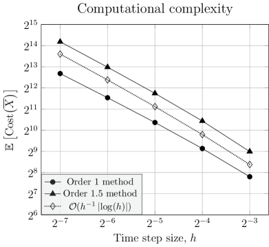
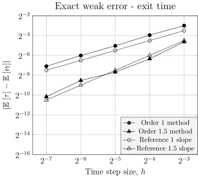
Figure 1. Error convergence rates and total computational complexity involved in implementing order 1 and order 1.5 adaptive methods for computing the exit time of the GBM process defined in Section 4.1.

4.2. Linear drift, cosine diffusion coefficient - 1D

For the SDE

$$\mathrm{d}X =0.1X\,\mathrm{d}t+0.3\big{(}\cos(X)+3\big{)}\,\mathrm{d}W$$

$$X(0) =4,$$

we study the exit time from the interval $D=(1,7)$. The reference solution to the mean exit time problem was computed by solving the Feynman–Kac PDE using the same numerical method as in the preceding example, yielding $\mathbb{E}\left[\tau\right]=5.504741$, rounded to 7 significant digits. We run $M=10^{7}$ simulations for our Monte Carlo estimates using the time-step parameter $h={2^{-3},2^{-4},2^{-5},2^{-6},2^{-7}}$. From Figure 2, the rates for strong error the computational cost are in close agreement with theory, and we observe that for the given sample size and range of $h$-values, the rate for the weak error is more reliably estimated by the sample mean of pairwise coupled realizations $\nu_{l}-\nu_{l-1}$ than the sample mean of $\mathbb{E}\left[\tau\right]-\nu_{\ell}$. The reason is that due to the pairwise coupling, the variance of $\nu_{l}-\nu_{l-1}$ is smaller than that of $\mathbb{E}\left[\tau\right]-\nu_{l}$.

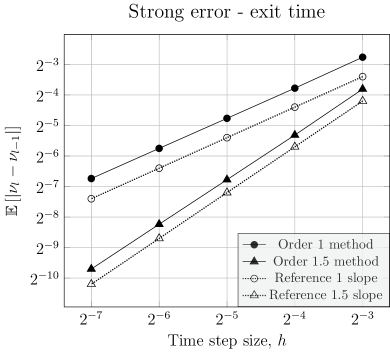
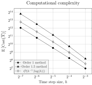
Figure 2. Error convergence rates and total computational complexity involved in implementing order 1 and order 1.5 adaptive methods for computing the exit time of SDE with linear drift coefficient and non-linear diffusion coefficient in Section 4.2.

We next consider two higher-dimensional exit time problems.

4.3. Linear drift, linear diffusion - 2D

We consider the SDE

$$\mathrm{d}X_{1} =0.05X_{2}\,\mathrm{d}t+0.2X_{1}\,\mathrm{d}W^{1}$$

$$\mathrm{d}X_{2} =0.05X_{1}\,\mathrm{d}t+0.2X_{2}\,\mathrm{d}W^{2}$$

with initial condition $X(0)=(3,3)^{\top}$, and we are interested in computing the exit time from the disk

$$D\coloneqq\{x\in\mathbb{R}^{2}\;\big{|}\;\sqrt{(x_{1}-3)^{2}+(x_{2}-3)^{2}}<3\}\,.$$ (43)

The reference solution to the mean exit time problem is computed by numerically solving the Feynman–Kac PDE, yielding $\mathbb{E}\left[\tau\right]=6.7737$, rounded to 5 significant digits. We estimate the sample moments using $M=10^{7}$ samples for $h=2^{-3},2^{-4},2^{-5},2^{-6},2^{-7}$. Figure 3 shows that the rates for the strong error and computational cost match those from theory and that for the given sample size, the weak error rate is more reliably estimated by samples of $\nu_{l}-\nu_{l-1}$ than by samples of $\mathbb{E}\left[\tau\right]-\nu_{l}$.

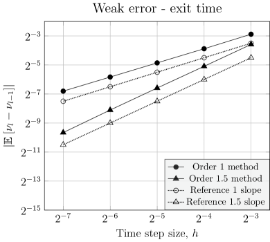
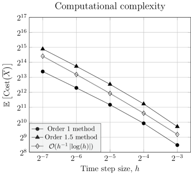
Figure 3. Error convergence rates and total computational cost involved in implementing order 1 and order 1.5 adaptive methods for computing the exit time of SDE with linear drift coefficient and linear diffusion coefficient in Section 4.3.

4.4. Linear drift, cosine diffusion - 2D

We consider the following two-dimensional SDE with linear drift and non-linear, diagonal diffusion coefficient:

$$\mathrm{d}X_{1} =0.1X_{2}\,\mathrm{d}t+0.25\big{(}\cos(X_{1})+3\big{)}\,\mathrm{d}W^{1}$$

$$\mathrm{d}X_{2} =0.1X_{1}\,\mathrm{d}t+0.25\big{(}\cos(X_{2})+3\big{)}\,\mathrm{d}W^{2},$$

and with initial condition $X(0)=(3,3)^{\top}$. Note that the components of the SDE are coupled through the drift term, similarly as for the SDE in Section 4.3. We compute the exit time of the SDE from the disk domain given by equation (43). The reference solution to the mean exit time problem is is computed by numerically solving the Feynman–Kac PDE, yielding $\mathbb{E}\left[\tau\right]=5.0853$, rounded to 5 significant digits. The weak and strong errors are estimated using $M=10^{7}$ samples for $h\in[2^{-3},2^{-7}]$, and, to reach the asymptotic regime of the computational cost, we have estimated it over the a range of smaller values, $h\in[2^{-4},2^{-14}]$, using $M=10^{3}$ (due to the bump in cost, and, luckily, cost estimates do not appear very sensitive to the sample size). Figure 4 shows that numerical results support theory and that for the given sample size, the weak error rate is more reliably estimated by the samples of $\nu_{l}-\nu_{l-1}$ than samples of $\mathbb{E}\left[\tau\right]-\nu_{l}$. Note also that the asymptotic regime for the computational cost is not reached at $h=2^{-7}$ for neither of the methods, but that the cost is proportional to $h^{-1}|log(h)|$ for smaller $h$-values.

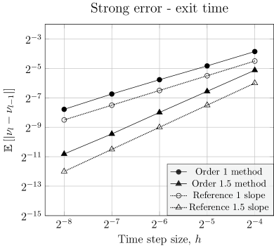
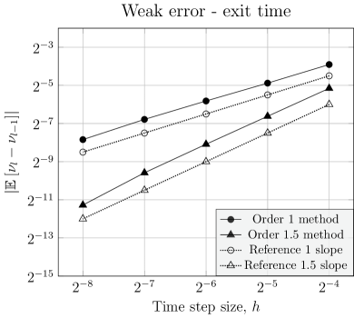
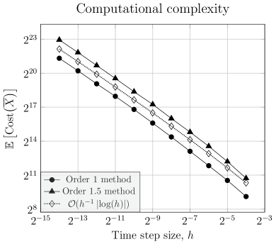
Figure 4. Error convergence rates and total computational cost involved in implementing order 1 and order 1.5 adaptive methods for computing the exit time of SDE with linear drift coefficient and non-linear diffusion coefficient in Section 4.4.

5. Conclusion

In this paper, we developed a tractable higher-order adaptive time-stepping method for the strong approximation of exit times of Itô-diffusions. We theoretically prove that the Milstein scheme combined with adaptive time-stepping with two different step sizes lead to a strong convergence rate of $\mathcal{O}(h^{1-})$, and that the strong order 1.5 Itô–Taylor scheme combined with adaptive time-stepping with three different step sizes lead to a strong convergence rates of $\mathcal{O}(h^{3/2-})$. We also showed that the expected computational cost for both methods are bounded by $\mathcal{O}(h^{-1}\left|\log(h)\right|)$. The fundamental idea in our approach, recurring in both of the aforementioned methods, is to use smaller step sizes as the numerical solution gets closer to the boundary of the domain, and to use higher-order integration schemes for better approximation of the state of the Itô-diffusion. This reduces both the magnitude of overshoot when the numerical solution exits the domain and the probability of the numerical solution missing an exit of the domain by the exact process.

There are several interesting ways to extend the current work. One direction would be to consider strong Itô–Taylor schemes of order $\gamma>3/2$ combined with adaptive time-stepping that employs more than two critical regions, i.e. for some $h\in(0,1)$, we consider time-step sizes finer than $h^{3}$ when the numerical solution is very close to the boundary $\partial D$. This way, the strong convergence rate can be further improved while maintaining a computational complexity that is tractable.

Although the higher-order adaptive method has been devised for improving the strong convergence rate of exit times of Itô-diffusions, the results easily extend to weak approximations of quantities of interest (QoI) that depend on the exit time and the state of the process:

$$\mathrm{QoI}\coloneqq f(\tau,X_{\tau})+\int_{0}^{\tau}g(s,X_{s})ds,$$

where we assume that $f,g$ are functions that are sufficiently smooth.

In the implementation of the higher-order adaptive time-stepping algorithm, we use smaller time-step sizes as the numerical process gets closer to the boundary of the domain which significantly increases the expected computational cost. Combination of multilevel Monte Carlo and adaptive time-stepping [22, 23, 9, 15, 24, 25] should significantly reduce the computational cost by using more Monte Carlo samples at the coarser level, where we use more degrees of freedom larger time-step size, and fewer Monte Carlo samples at the finer level, where we use a smaller time-step size. To implement the MLMC method, one requires the fine and the coarse trajectories of the stochastic process to be strongly coupled while also ensuring that the telescoping-sum property is satisfied. A smart way to couple solutions of the Euler–Maruyama method on non-nested adaptive meshes has been developed in [15], and it would be interesting to study how extensible that approach is to higher-order methods, using for instance the coupling procedure in [21, Example 1.1].

Finally, in [14], a new multilevel Monte Carlo methodology to compute the mean exit time or a QoI that depends on the exit time of a stochastic process was developed. The new MLMC method reduces the multilevel variance by computing the approximate conditional expectation once the coarse or fine trajectory has exited the domain. Combining our ideas on higher-order, adaptive time-stepping with the conditional MLMC method has the potential to reduce the computational cost of exit time simulations even further. This makes an interesting problem for future research.

Appendix A Theoretical results

Lemma A.1.

Let Assumptions A and B hold, and for the initial condition $x_{0}\in D$ of the SDE (2) let $\lambda:=d(x_{0},\partial D)/2$ and let $\bar{\delta}>0$ be sufficiently small such that $\bar{\delta}<\bar{R}_{D}/2$ and $d(x_{0},\Gamma_{2\bar{\delta}})>\lambda$, where we recall that $\Gamma_{2\delta}:=D_{2\delta}\setminus D_{-2\delta}$ for $\delta\in[0,\bar{\delta}]$. Then, there exists a constant $C_{p}>0$ such that the absorbing-boundary Fokker–Planck equation (34) satisfies

$$\max_{(t,x)\in[0,T]\times\overline{\Gamma}_{2\delta}}p(t,x;\delta)\leq 4C_{p}\delta,\qquad\forall\delta\in[0,\bar{\delta}],$$

where $C_{p}$ is independent of $\delta$.

Proof.

Following [10, Chapter 3.7], the solution of the Fokker–Planck equation can be decomposed into the sum of two functions:

$$p(t,x;\delta)=\widehat{\Gamma}(t,x;0,x_{0})+V(t,x;\delta),$$

where $\widehat{\Gamma}$ denotes a fundamental solution to a global parabolic extension of the Fokker-Planck PDE from the domain $D_{2\bar{\delta}}$ to $\mathbb{R}^{d}$ (making it a fundamental solution for $p(t,x;\delta)$ for every $\delta\in[0,\bar{\delta}]$) and $V$ is a boundary correction term solving the Fokker-Planck equation

$$\partial_{t}V =-\nabla\cdot(aV)+\frac{1}{2}\nabla\cdot\!\left(bb^{\top}\nabla V\right) \text{in}\quad(0,T]\times D_{2\delta},$$

$$V(t,x;\delta) =-\widehat{\Gamma}(t,x;0,x_{0}) \text{on}\quad(0,T]\times\partial D_{2\delta}$$

$$V(0,x;\delta) =0 \quad x\in\overline{D}_{2\delta}.$$

Assumption B and [10, Chapter 1.6] implies that $\widehat{\Gamma}\in C^{1,2}_{b}([0,T]\times\overline{\Gamma}_{2\bar{\delta}})$. Let

$$C_{\widehat{\Gamma}}:=\max_{(x,t)\in[0,T]\times\overline{\Gamma}_{2\bar{\delta}}}\widehat{\Gamma}+|\partial_{t}\widehat{\Gamma}|+|\nabla\widehat{\Gamma}|+|\nabla^{2}\widehat{\Gamma}|,$$

and note that also the boundary data for $V$,

$$\varphi(t,x;\delta)=\begin{cases}-\widehat{\Gamma}(t,x;0,x_{0})&(t,x)\in(0,T]\times\partial D_{2\delta}\\ 0&(t,x)\in\{0\}\times\overline{D}_{2\delta}\end{cases}$$

satisfies $\varphi\in C^{1,2}_{b}\Big{(}\big{(}(0,T]\times\partial D_{2\delta}\big{)}\cup\big{(}\{0\}\times\overline{D}_{2\delta}\big{)}\Big{)}$ with the following uniform upper bound over all points on the boundary domain

$$|\varphi|+|\partial_{t}\varphi|+|\nabla\varphi|+|\nabla^{2}\varphi|\leq C_{\widehat{\Gamma}}\qquad\forall\delta\in[0,\bar{\delta}].$$

The boundary gradient of $V$ will be bounded using [28, Lemma 10.1], so we need to verify that the lemma applies to $V$ for any $\delta\in[0,\bar{\delta}]$. Note first that by the maximum principle, it holds that $|V|\leq C_{\widehat{\Gamma}}$ for all $\delta\in[0,\bar{\delta}]$. Assumption A and $\bar{R}_{D}<\mathrm{reach}(D)/2$ further implies that $D_{2\delta}$ satisfies the uniform ball condition with $\mathrm{reach}(D_{2\delta})>\mathrm{reach}(D)/2>\bar{R}_{D}$ for all $\delta\in[0,\bar{\delta}]$. Therefore, any point $x\in\partial D_{2\delta}$ for any $\delta\in[0,\bar{\delta}]$ satisfies the infinite exterior cylinder condition with radius $\tilde{r}:=\bar{R}_{D}$, cf. [28, Lemma 10.1]. Thanks to Assumption B there exists a constant $C_{ab}>0$ that depends on the supremum of the SDE coefficents $a$ and $b$ and their first and second partial derivatives on $D_{\bar{R}_{D}}$ such that the left-hand side of [28, inequality (10.6)] is bounded from above by

$$g_{L}(p):=1+\Big{(}\widehat{C}_{b}+C_{ab}(C_{\widehat{\Gamma}}+1)\Big{)}|p|\quad\text{for}\quad p\in\mathbb{R}^{d}$$

while the $\mu$-scaled Bernstein coefficient on the right-hand side of the same inequality is bounded from below by $g_{R}(p;\mu):=\mu\hat{c}_{b}|p|^{2}$, where $\mu>0$ is the scaling parameter and $\widehat{C}_{b}>\hat{c}_{b}>0$ are defined in Assumption B. This implies that one can find constants $\mu,p_{0}>0$ that are independent of $\delta$ such that

$$g_{L}(p)\leq g_{R}(p;\mu)\qquad\text{for all}\quad p\in\mathbb{R}^{d}\quad\text{such that}\quad|p|\geq p_{0}.$$

We have shown that [28, Lemma 10.1] applies, which means there exists a constant $C_{V}>0$ that depends on $\mu,p_{0}$, the uniform infinite exterior cylinder radius $\tilde{r}$ and $C_{\widehat{\Gamma}}$ such that

$$\sup_{(t,x,y)\in[0,T]\times D_{2\delta}\times\partial D_{2\delta}}|V(t,x;\delta)-V(t,y;\delta)|\leq C_{V}|x-y|$$

holds for all $\delta\in[0,\bar{\delta}]$. And since

$$|p(t,x;\delta)-p(t,y;\delta)|\leq|\widehat{\Gamma}(t,x)-\widehat{\Gamma}(t,y)|+|V(t,x;\delta)-V(t,y;\delta)|,$$

and $p(t,y;\delta)=0$ for $y\in\partial D_{2\delta}$, we conclude that

$$\max_{(t,x)\in[0,T]\times\overline{\Gamma}_{2\delta}}p(t,x;\delta)\leq\underbrace{(C_{\widehat{\Gamma}}+C_{V})}_{=:C_{p}}\max_{x\in\overline{\Gamma}_{2\delta}}d(x,\partial D_{2\delta})\leq 4C_{p}\delta.$$

∎

Lemma A.2.

For a domain $D$ satisfying Assumption A and $R={reach}(D)/2)$, the mapping $\mathcal{I}:[-R,R]\to[0,\infty)$ defined by

$$\mathcal{I}(r)=\int_{\partial D_{r}}dS(x),$$

satisfies that $\max_{r\in[-R,R]}\mathcal{I}(r)<\infty$.

Proof.

For each $r\in[-R,R]$ we recall that $\partial D_{r}$ is $C^{3}$ and there exists a constant $C_{r}>0$ such that

$$\mathcal{I}(r)\leq C_{r}\int_{D_{R}}dx,$$

cf. [28, Lemma 6.36]. To obtain a uniform upper bound we introduce the following mapping on the domain $\overline{\Gamma}_{R}=\{x\in D_{R}\mid d(x,\partial D_{R})\leq 2R\}$:

$$d(x):=\begin{cases}d(x,D)&\text{if}\quad x\in D\cap\overline{\Gamma}_{R}\\ -d(x,D)&\text{if}\quad x\in D^{C}\cap\overline{\Gamma}_{R}.\end{cases}$$

A small extension of [13, Lemma 14.16] yields that $d\in C^{3}(\overline{\Gamma}_{R})$ and that for any $x\in\partial D_{r}$ and $r\in[-R,R]$,

$$-\nabla d(x)=n_{D}(\pi_{r}^{-1}(x))=n_{D_{r}}(x),$$

where we recall that $n_{D_{r}}$ denotes the outward pointing normal on the boundary $\partial D_{r}$. For any $r\in[-R,R]$ the divergence theorem yields

$$\begin{split}|\mathcal{I}(r)-\mathcal{I}(0)|&=\left|\int_{\partial D_{r}}|\nabla d(x)|^{2}dS(x)-\int_{\partial D_{0}}|\nabla d(x)|^{2}dS(x)\right|\\ &\leq\int_{\Gamma_{R}}|\Delta d(x)|dx<\infty,\end{split}$$

where the last inequality follows from $\Delta d\in C^{1}(\overline{\Gamma}_{R})$. We conclude that

$$\max_{r\in[-R,R]}\mathcal{I}(r)\leq\mathcal{I}(0)+\max_{r\in[-R,R]}|\mathcal{I}(r)-\mathcal{I}(0)|<\infty.$$

∎

Appendix B Computational cost for the order 1 method - 1D Wiener process

In this section we use a more fundamental approach to deriving an upper bound for the computational cost of implementing the order 1 adaptive method for a one-dimensional Wiener process $W(t)$ exiting the interval $(a,b)$. This is possible thanks to the availability of the joint density for the state of the process $W(t)$ and its running maximum/minimum.

Let $\overline{W}(t)$ denote the continuous time extension of the discretely sampled Wiener process. For $t>s\geq 0$, let $M_{W}(s,t)$ and $m_{W}(s,t)$ denote the running maximum and the running minimum of the one-dimensional Wiener process $W(t)$, respectively, over the interval $[s,t]$, i.e.

$$M_{W}(s,t) \coloneqq\sup_{r\in[s,t]}\big{(}W(r)-W(s)\big{)}$$

$$m_{W}(s,t) \coloneqq\inf_{r\in[s,t]}\big{(}W(r)-W(s)\big{)}$$

Let the shorthands $M_{W}(t)$ and $m_{W}(t)$ represent the running maximum and the running minimum of the Wiener process over the interval $[0,t]$, respectively. Recall that the running maximum and the negative of the running minimum of the Wiener process have the same distribution, cf. [26, Section 3.6].

The threshold parameter $\delta(h)$, for all $h\in(0,1)$, is defined as

$$\delta(h)\coloneqq\sqrt{4h\log(h^{-1})}$$ (44)

We construct the set $A$ to bound the strides of the running maximum and the running minimum of the Wiener process

$$\begin{split}A&\coloneqq\left\{\omega\in\Omega\;\big{|}\;M_{W}(t_{n},t_{n+1})\leq\delta,\forall n\in\{0,1,\ldots,N-1\}\right\}\\ &\qquad\cap\left\{\omega\in\Omega\;\big{|}\;m_{W}(t_{n},t_{n+1})\geq-\delta,\forall n\in\{0,1,\ldots,N-1\}\right\}\end{split}$$ (45)

It can be shown for all $h<e^{-1}$, in a manner similar to the proof argument for Lemma 3.3, and for the choice of $\delta$ given by equation (44) that

$$\mathbb{P}\!\left(A^{C}\right)=\mathcal{O}(h\left|\log(h)\right|^{-1/2})$$

Proposition B.1 (Computational cost for the order 1 method - 1D Wiener process).

For a sufficiently small step size parameter $h>0$, the joint probability density of the tuple of random variables $(W(t),M_{W}(t))$ given by

$$\rho_{(W(t),M_{W}(t))}(w,m)\coloneqq\sqrt{\frac{2}{\pi}}\frac{2m-w}{t^{3/2}}\exp\left(-\frac{(2m-w)^{2}}{2t}\right),\quad m\geq 0,\;w\leq m$$

is well-defined for any $t\in[h,T]$ and

$$\sup_{(t,w,m)\in[h,T]\times[b-\delta,b)\times[b-\delta,b+\delta]}\rho_{(W(t),M_{W}(t))}(w,m)<\infty\,.$$

It further holds that

$$\mathbb{E}\left[\mathrm{Cost}\!\left(\overline{W}\right)\right]=\mathcal{O}(h^{-1}\left|\log(h)\right|)\,.$$

Proof.

Based on the size of the strides taken by the Wiener process, the computational cost can be decomposed as follows:

$$\mathbb{E}\left[\mathrm{Cost}\!\left(\overline{W}\right)\right]=\mathbb{E}\left[\mathrm{Cost}\!\left(\overline{W}\right)\mathbbm{1}_{A^{C}}\right]+\mathbb{E}\left[\mathrm{Cost}\!\left(\overline{W}\right)\mathbbm{1}_{A}\right]\eqqcolon I+II,$$

where the set $A$ was defined in (45). For term $I$, note that the upper bound on the number of time-steps that can be taken by the Wiener process before it exits the domain, using the order 1 adaptive time-stepping method, is $T/h^{2}$. From this, we obtain

$$I =\mathbb{E}\left[\mathrm{Cost}\!\left(\overline{W}\right)\mathbbm{1}_{A^{C}}\right]\leq\frac{T}{h^{2}}\mathbb{E}\left[\mathbbm{1}_{A^{C}}\right]=\frac{T}{h^{2}}\mathbb{P}\!\left(A^{C}\right)=\mathcal{O}(h^{-1}\left|\log(h)\right|^{-1/2})\,.$$

For term $II$, we can write the computational cost as

$$II =\mathbb{E}\left[\mathrm{Cost}\!\left(\overline{W}\right)\mathbbm{1}_{A}\right]\leq\frac{T}{h}+\int_{h}^{T}\frac{\mathbb{E}\left[\mathbbm{1}_{\{\nu>t\}\cap\{\Delta t(\overline{W}(t))=h^{2}\}\cap A}\right]}{h^{2}}\mathrm{d}t\,.$$

Note that

$$\{\nu>t\}\,{\cap}\,\{\Delta t(\overline{W}(t))=h^{2}\}\,{\cap}\,A\,{\subset}\\ \Big{(}\{M_{W}(t)\in[b-\delta,b+\delta)\}\,{\cap}\,\{W(t)\in[b-\delta,b)\}\Big{)}\,{\cup}\\ \Big{(}\{m_{W}(t)\in(a-\delta,a+\delta]\}\,{\cap}\,\{W(t)\in(a,a+\delta]\}\Big{)}\,.$$

For any $h<\min(e^{-1},T)$, $t\in[h,T]$ and $(w,m)\in[b-\delta,b)\times[b-\delta,b+\delta]$, it holds that

$$\rho_{(W(t),M_{W}(t))}(w,m) =\sqrt{\frac{2}{\pi}}\frac{(2m-w)}{t^{3/2}}\exp\left(-\frac{(2m-w)^{2}}{2t}\right)$$

$$\leq\sqrt{\frac{2}{\pi}}\frac{b+3\delta}{t^{3/2}}\exp\left(-\frac{(b-\delta)^{2}}{2t}\right)$$

$$\leq\max_{t\in[h,T]}\sqrt{\frac{2}{\pi}}\frac{b+6e^{-1/2}}{t^{3/2}}\exp\left(-\frac{(b-2e^{-1/2})^{2}}{2t}\right)$$

$$=:C_{\rho}^{b}<\infty.$$

Using a similar argument, we can bound the joint probability density function $\rho_{(W(t),m_{W}(t))}(w,m)$ uniformly for all $(w,m)\in(a,a+\delta]\times[a-\delta,a+\delta]$ and $t\in[h,T]$ by a positive constant $C_{\rho}^{a}<\infty$. From the above results, we obtain that

$$II \leq\frac{T}{h}+\frac{C_{\rho}^{a}\delta^{2}(T-h)}{h^{2}}+\frac{C_{\rho}^{b}\delta^{2}(T-h)}{h^{2}}=\mathcal{O}(h^{-1}\left|\log(h)\right|)\,.$$

∎

Acknowledgments

Thanks to Mike Giles for remarks and discussions on the manuscript, particularly for the very nice idea to use the absorbing-boundary Fokker–Planck equation in the proof of the computational cost of the adaptive methods. This improved our computational cost result considerably!

We would also like to thank Snorre Harald Christensen, Kenneth Karlsen, Peter H.C. Pang and Nils Henrik Risebro for helpful discussions on parabolic and elliptic PDE.

Financial support

This work was supported by the Mathematics Programme of the Trond Mohn Foundation.

References

- [1] Gerold Alsmeyer, On the markov renewal theorem, Stochastic processes and their applications 50 (1994), no. 1, 37–56.
- [2] Santiago Badia and Francesc Verdugo, Gridap: An extensible finite element toolbox in julia, Journal of Open Source Software 5 (2020), no. 52, 2520.
- [3] Paolo Baldi, Stochastic calculus, Stochastic Calculus, Springer, 2017, pp. 215–254.
- [4] Christian Bayer, Raúl Tempone, and Sören Wolfers, Pricing american options by exercise rate optimization, Quantitative Finance 20 (2020), no. 11, 1749–1760.
- [5] Bruno Bouchard, Stefan Geiss, and Emmanuel Gobet, First time to exit of a continuous Itô process: General moment estimates and -convergence rate for discrete time approximations, Bernoulli 23 (2017), no. 3, 1631–1662, Publisher: Bernoulli Society for Mathematical Statistics and Probability.
- [6] Mark Broadie, Paul Glasserman, and Steven Kou, A continuity correction for discrete barrier options, Mathematical Finance 7 (1997), no. 4, 325–349.
- [7] Jérémy Dalphin, Some characterizations of a uniform ball property, ESAIM: proceedings and surveys 45 (2014), 437–446.
- [8] Madalina Deaconu, Samuel Herrmann, and Sylvain Maire, The walk on moving spheres: a new tool for simulating brownian motion’s exit time from a domain, Mathematics and Computers in Simulation 135 (2017), 28–38.
- [9] Wei Fang and Michael B Giles, Adaptive euler–maruyama method for sdes with nonglobally lipschitz drift, The Annals of Applied Probability 30 (2020), no. 2, 526–560.
- [10] Avner Friedman, Partial differential equations of parabolic type, Prentice-Hall, Inc., Englewood Cliffs, N.J., 1964. MR 0181836
- [11] by same author, Stochastic differential equations and applications. Vol. 1, Probability and Mathematical Statistics, Vol. 28, Academic Press, New York-London, 1975. MR 0494490
- [12] David Gilbarg and Lars Hörmander, Intermediate schauder estimates, Archive for Rational Mechanics and Analysis 74 (1980), no. 4, 297–318.
- [13] David Gilbarg and Neil S Trudinger, Elliptic partial differential equations of second order, vol. 224, springer, 2015.
- [14] Michael B Giles and Francisco Bernal, Multilevel estimation of expected exit times and other functionals of stopped diffusions, SIAM/ASA Journal on Uncertainty Quantification 6 (2018), no. 4, 1454–1474.
- [15] Michael B. Giles, Christopher Lester, and James Whittle, Non-nested Adaptive Timesteps in Multilevel Monte Carlo Computations, Monte Carlo and Quasi-Monte Carlo Methods (Cham) (Ronald Cools and Dirk Nuyens, eds.), Springer Proceedings in Mathematics & Statistics, Springer International Publishing, 2016, pp. 303–314 (en).
- [16] Emmanuel Gobet, Weak approximation of killed diffusion using euler schemes, Stochastic Process. Appl. 87 (2000), no. 2, 167–197.
- [17] by same author, Euler schemes and half-space approximation for the simulation of diffusion in a domain, ESAIM Probab. Stat. 5 (2001), 261–297.
- [18] Emmanuel Gobet and Stéphane Menozzi, Exact approximation rate of killed hypoelliptic diffusions using the discrete Euler scheme, Stochastic Processes and their Applications 112 (2004), no. 2, 201–223 (en).
- [19] by same author, Stopped diffusion processes: Boundary corrections and overshoot, Stochastic Processes and their Applications 120 (2010), no. 2, 130–162 (en).
- [20] Desmond J. Higham, Xuerong Mao, Mikolaj Roj, Qingshuo Song, and George Yin, Mean Exit Times and the Multilevel Monte Carlo Method, SIAM/ASA Journal on Uncertainty Quantification 1 (2013), no. 1, 2–18, Publisher: Society for Industrial and Applied Mathematics.
- [21] Håkon Hoel and Sebastian Krumscheid, Central limit theorems for multilevel monte carlo methods, Journal of Complexity 54 (2019), 101407.
- [22] Håkon Hoel, Erik von Schwerin, Anders Szepessy, and Raúl Tempone, Adaptive multilevel monte carlo simulation, Numerical Analysis of Multiscale Computations, Springer, Berlin, Heidelberg, 2012, pp. 217–234.
- [23] Håkon Hoel, Erik Von Schwerin, Anders Szepessy, and Raúl Tempone, Implementation and analysis of an adaptive multilevel monte carlo algorithm, Monte Carlo Methods and Applications 20 (2014), no. 1, 1–41.
- [24] Grigoris Katsiolides, Eike H Müller, Robert Scheichl, Tony Shardlow, Michael B Giles, and David J Thomson, Multilevel monte carlo and improved timestepping methods in atmospheric dispersion modelling, Journal of Computational Physics 354 (2018), 320–343.
- [25] Cónall Kelly and Gabriel J Lord, Adaptive time-stepping strategies for nonlinear stochastic systems, IMA Journal of Numerical Analysis 38 (2018), no. 3, 1523–1549.
- [26] Fima C Klebaner, Introduction to stochastic calculus with applications, World Scientific Publishing Company, 2012.
- [27] Peter E Kloeden and Eckhard Platen, Stochastic differential equations, Numerical solution of stochastic differential equations, Springer, 1992, pp. 103–160.
- [28] Gary M. Lieberman, Second order parabolic differential equations, World Scientific Publishing Co., Inc., River Edge, NJ, 1996. MR 1465184
- [29] Fabian Merle and Andreas Prohl, A posteriori error analysis and adaptivity for high-dimensional elliptic and parabolic boundary value problems, Numerical Analysis preprint server at University of Tübingen (2022), https://na.uni-tuebingen.de/preprints.shtml.
- [30] Peter Mörters and Yuval Peres, Brownian motion, vol. 30, Cambridge University Press, 2010.
- [31] Mervin E Muller, Some continuous monte carlo methods for the dirichlet problem, The Annals of Mathematical Statistics (1956), 569–589.
- [32] Thomas Müller-Gronbach, The optimal uniform approximation of systems of stochastic differential equations, aoap 12 (2002), no. 2, 664–690 (en).
- [33] T. Naeh, M. M. Kł osek, B. J. Matkowsky, and Z. Schuss, A direct approach to the exit problem, SIAM J. Appl. Math. 50 (1990), no. 2, 595–627. MR 1043605
- [34] Andreas Neuenkirch, Michaela Szölgyenyi, and Lukasz Szpruch, An adaptive euler–maruyama scheme for stochastic differential equations with discontinuous drift and its convergence analysis, SIAM Journal on Numerical Analysis 57 (2019), no. 1, 378–403.
- [35] Zeev Schuss, Theory and applications of stochastic differential equations, Wiley Series in Probability and Statistics, John Wiley & Sons, Inc., New York, 1980. MR 595164
- [36] Francesc Verdugo and Santiago Badia, The software design of gridap: A finite element package based on the julia JIT compiler, Computer Physics Communications 276 (2022), 108341.
- [37] E Weinan, Tiejun Li, and Eric Vanden-Eijnden, Applied stochastic analysis, vol. 199, American Mathematical Soc., 2021.
- [38] Larisa Yaroslavtseva, An adaptive strong order 1 method for sdes with discontinuous drift coefficient, Journal of Mathematical Analysis and Applications 513 (2022), no. 2, 126180.