Differential evolution variants for Searching $D$- and $A$-optimal designs

Abstract

Optimal experimental design is an essential subfield of statistics that maximizes the chances of experimental success. The $D$- and $A$-optimal design is a very challenging problem in the field of optimal design, namely minimizing the determinant and trace of the inverse Fisher information matrix. Due to the flexibility and ease of implementation, traditional evolutionary algorithms (EAs) are applied to deal with a small part of experimental optimization design problems without mathematical derivation and assumption. However, the current EAs remain the issues of determining the support point number, handling the infeasible weight solution, and the insufficient experiment. To address the above issues, this paper investigates differential evolution (DE) variants for finding $D$- and $A$-optimal designs on several different statistical models. The repair operation is proposed to automatically determine the support point by combining similar support points with their corresponding weights based on Euclidean distance and deleting the support point with less weight. Furthermore, the repair operation fixes the infeasible weight solution into the feasible weight solution. To enrich our optimal design experiments, we utilize the proposed DE variants to test the $D$- and $A$-optimal design problems on 12 statistical models. Compared with other competitor algorithms, simulation experiments show that LSHADE can achieve better performance on the $D$- and $A$-optimal design problems.

1 Introduction

The sub-field of optimal experimental design is an increasingly important statistical research topic for two reasons. The first and traditional reason is that experimental costs are always increasing and a well designed study can provide the most accurate inference at minimum cost [1]. The second reason is its newly found applications to devise optimal subsampling schemes to make inference from big data based on the selected sample. Optimal design techniques and ideas have been increasingly applied across disciplines to save experimental costs [2]. Some examples are in the design of dose-response experiments [3], petroleum engineering [4], clinical pharmacology experiments [5], and image retrieval [6], among many others. These optimal experimental designs are model-based and are found by optimizing the design criterion, which is usually formulated as a convex function of the Fisher’s information matrix defined below. This matrix measures the worth of the design and depends on the unknown model parameters if the model is nonlinear. $D$- and $A$-locally-optimal designs are among the most popular designs for estimating model parameters but there are other design criteria with different objectives. Fundamentals of optimal design construction are given in [7, 8, 9] and [10] compared robustness properties of optimal designs under different models and criteria assumptions.

The traditional approach in the statistics literature leans heavily on mathematical derivations. Our experience is that such an approach can be limited, especially when we have a regression model complicated. Some of the algorithms in the statistics literature have a proof of convergence but in practice, they may not converge and get trapped in local optima [11]. Other problems are usually due to the fact that most proofs are for linear models and have the assumption that the criterion or objective function is differentiable. Nature-inspired metaheuristic algorithms have emerged as powerful tools to solve all kinds of optimization problems without technical assumptions imposed on the problem [12]. Examples of such evolutionary algorithms (EAs) and nature-inspired algorithms are simulated annealing (SA) [13, 14], genetic algorithm (GA) [15, 16], particle swarm optimization (PSO) [17, 18], Differential evolution (DE) [19] and some of them have been applied to solve $D$- and $A$-optimal design problems [11]. However, it is hard to know the real support point number and appears many similar support points when the design variables can be optimized by naive EAs. It is also challenging that EAs should seek feasible solutions on the support points and their corresponding weights that must be satisfied with the condition of the sum of the corresponding weights to 1. And it is insufficient that existing naive EAs are utilized to test on a small number of optimal design problems.

In this paper, we investigates DE variants for finding $D$- and $A$-optimal designs on several different statistical models. To address above issues, we propose the repair operation to combine similar support points with their corresponding weights based on Euclidean distance and delete the corresponding support point with less weight to automatically recognize the number of support points. To solve the infeasible weight solutions of optimal design problems, the repair operation ensures that the infeasible weight solutions are repaired into the feasible weight solutions. To enrich the $D$- and $A$-optimal design experiment, we adopt the advanced DE variants: JADE [20], CoDE [21], SHADE [22], and LSHADE [23] to test the performance for the $D$- and $A$-optimal design. Simulation experiments of 12 statistical models are shown that LSHADE obtains better performance on the $D$- and $A$-optimal problems among comparative algorithms.

The rest paper is organized as follows: Section 2 describes the related work about the approximate design and the information matrix, the $D$-optimal design, the $A$-optimal design, and the traditional Differential evolution. In Section 3, we utilize the proposed DE variants with the repair operation to solve the $D$- and $A$-optimal design. In Section 4, the simulated experiments of 12 statistical models are conducted on the $D$- and $A$-optimal design criterion, the experiment result of EAs are compared, and we conduct the discussion and analysis. Section 5 gives a conclusion.

2 Statistical Background

2.1 Statistical models, approximate designs and information matrices

Our statistical models have the form:

$$Y=\eta\left({{\bf{x}},\theta}\right)+\varepsilon,{\rm{}}{\bf{x}}\in{\bf{X},}$$ (1)

where ${Y}$ is univariate response and the mean response function $\eta\left({{\bf{x}},\theta}\right)$ is a known continuous function of a vector of input variables or design variables $\bf{x}$ assumed to belong a user-specified compact design space $\bf{X}$. The vector of unknown model parameters in the model is ${\theta}$ and has dimension ${p}$ and the error ${\varepsilon}$ is error term with zero mean and constant variance. All errors are assumed to be identically and independently distributed, but the methodology can be directly extended to the case when errors are independent with a known heteroscedastic structure.

Design problems concern choosing the combinations of the levels of the input variables so that the model unknown parameter $\theta$ is estimated as precisely as possible, subject to fixed number of observations $N$ determined by the budget. The optimization problem then determines the optimal number of design points, the optimal values of the input values at each point and the number of replicates at each point. In practice, approximate designs are used because they are easier to find and study [24]. Approximate designs are simply probability measures $\xi$ represented by ${\xi{\rm{=}}\left\{{\left({{{\bf{x}}_{i}},{\omega_{i}}}\right),i=1,2,...,m}\right\}}$, where each ${{{\bf{x}}_{i}}\in{\bf{X}}}$ is a support point and ${{\omega_{i}}>0}$ is the proportion of total observations to be taken at ${{\bf{x}}_{i}}$, subject to the constraint ${\sum\limits_{i=1}^{m}{{\omega_{i}}}=1}$. They are then implemented by taking $[N*\omega_{i}]$ observations at ${\bf x_{i}},i=1,2,\ldots,m$, subject to $[N*\omega_{1}]+[N*\omega_{2}]+...+[N*\omega_{m}]=N$ and $[s]$ is the positive integer nearest to s.

Following convention, the worth of a design is measured by its Fisher information matrix [7, 25]. This is because the covariance matrix of the maximum likelihood estimates of $\theta$ is inversely proportional to the determinant of the information matrix and so choosing input variables to make the information matrix large in some sense is equivalent to making the covariance matrix small. For the approximate design ${\xi}$, its normalized $p\times p$ information matrix is given by

$${\bf{M}}\left({\xi,\theta}\right)=\sum\limits_{i=1}^{m}{{\omega_{i}}}{\bf{M}}\left({{{\bf{x}}_{i}},\theta}\right)$$ (2)

where

$${\bf{M}}\left({{{\bf{x}}_{i}},\theta}\right)=\frac{{\partial\eta\left({{{\bf{x}}_{i}},\theta}\right)}}{{\partial\theta}}\frac{{\partial\eta\left({{{\bf{x}}_{i}},\theta}\right)}}{{\partial{\theta^{\rm{T}}}}}.$$ (3)

The next two subsections present two common design optimality criteria for estimating model parameters. We note that they are formulated as convex functional functions of the information matrix so that the optimum design found is globally optimum and we can use the directional derivative of the convex function to confirm a design optimality. We also note that if the mean response is a nonlinear function of $\theta$, then the information matrix contains the unknown parameters.

2.2 The $D$- and $A$-optimality criteria

Inference for a single parameter can be based on a confidence intervals and shorter intervals imply more accurate inference. Similarly, for two or more parameters, smaller area of the confidence region or smaller volume of the confidence ellipsoid indicates more accurate estimates. Since the volume of the confidence ellipsoid is inversely proportional to the determinant of the information matrix [25], a design that maximizes the determinant of the information matrix among all approximate designs on ${\bf X}$ is desirable. For nonlinear models, the determinant depends on the unknown model parameters $\theta$ so it cannot be optimized directly. In practice, the user uses a prior guess of its value (nominal value) and the resulting design ${\xi_{\theta}^{*}}$ is called locally $D$-optimal. Specifically,

$$\xi_{\theta}^{*}=\text{arg min}~{}\text{log}~{}\text{det}~{}{{\bf{M}}^{-1}}{\rm{(}}\xi{\rm{,}}\theta{\rm{}})$$

and the minimization is over all approximate designs $\xi$ in ${\bf X}$. Let $\bar{\xi}_{x}$ be the design supported at the point ${x}$ and let $\xi^{\prime}=(1-\alpha)\xi+\alpha\bar{\xi}_{x}$. Then

$${\bf{M}}(\xi^{\prime})=(1-\alpha){\bf{M}}(\xi)+\alpha{\bf{M}}(\bar{\xi}_{x})=(1-\alpha){\bf{M}}(\xi)+\alpha{f(x)f(x)^{T}}$$ (4)

and it follows that if $\psi(x,\xi)=\text{log~{}det}({{\bf{M}}^{-1}}{\rm{(}}\xi{\rm{,}}\theta{\rm{)}}$, its directional derivative is

$$\begin{array}[]{l}\varphi(x,\xi)=\mathop{\lim}\limits_{\alpha\to{0^{+}}}\frac{1}{\alpha}[\psi\{{\bf{M}}(\xi^{\prime},\theta)\}-\psi\{{\bf{M}}(\xi,\theta)\}].\\ \end{array}$$ (5)

The equivalence theorem [24] states that a design $\xi^{*}$ is $D$-optimal if and only if the minimum of the directional derivative $\varphi(x,{\xi^{*}})\geq 0$ for all $x$ in X, with inequity at the support points of the design. The sensitive function of the design $\xi$ is:

$$\begin{array}[]{l}S(x,{\xi_{D}})=-\varphi(x,{\xi_{D}})\\ =trace({\bf{M}}(\bar{\xi},\theta){{\bf{M}}^{-1}}({\xi_{D}},\theta))-p\\ =trace(f(x)f{(x)^{T}}{{\bf{M}}^{-1}}({\xi_{D}},\theta))-p\\ =f{(x)^{T}}{{\bf{M}}^{-1}}({\xi_{D}},\theta)f(x)-p.\end{array}$$ (6)

The practical implication is that $D$-optimality of a design $\xi$ can now be verified by plotting its sensitivity function over the design space and determining if it is the conditions of the equivalence theorem. If the design space is uni-dimensional, the sensitivity plot provides an easy visual confirmation of whether the design is $D$-optimal. If a design is not optimal, a $D$-efficiency lower bound of the design $\xi$ can be deduced from properties of a convex functional to be:

$$D\_Eff(\xi)=\exp(-\frac{{\max(S(x,{\xi_{D}}))}}{p});$$ (7)

see details in [26] and [25]. The usefulness of the bound is that it provides an easy assessment how close a design is to the optimum without knowing the optimum. For example, when an algorithm to find a $D$-optimal design is terminally prematurely or stalled, the $D$-efficiency lower bound can be computed directly. If the design has a high efficiency, it may suffice for practical purposes and there is no need to find the true optimum.

The $A$-optimality design criterion minimizes the sum of the variances of the estimated parameters in the model. This is equivalent to find a design that minimizes the trace of the inverse of the information matrix over all approximate designs on ${\bf X}$. The resulting design is $A$-optimal

$$\xi_{\theta}^{*}=\text{arg min}~{}\text{trace}~{}{{\bf{M}}^{-1}}{\rm{(}}\xi{\rm{,}}\theta{\rm{}})$$

and a similar argument. A similar argument shows that the sensitivity function of a design under the $A$-optimality criterion is

$$S(x,{\xi_{A}})={\mathop{\rm trace}\nolimits}({\bf{M}}(\bar{\xi},\theta){{\bf{M}}^{-2}}({\xi_{A}},\theta))-{\mathop{\rm trace}\nolimits}({{\bf{M}}^{-1}}({\xi_{A}},\theta))$$

and a design $\xi$ is $A$-optimal if and only if $S(x,\xi)$ is bounded above by 0 for all $x\in{\bf X}$, with equality at the support points of $\xi$. Likewise, the $A$-efficiency lower bound of a design $\xi$ can be directly derived to be

$$A\_Eff(\xi)=1-\frac{{\max(S(x,{\xi_{A}}))}}{{trace\left({{{\bf{M}}^{-1}}({\xi_{A}},\theta)}\right)}}$$ (8)

In our work, if a design has at least a $D$-efficiency or $A$-efficiency of 95%, we accept the design as close enough to the optimum.

2.3 The traditional DE

Differential Evolution (DE) is a competitive evolutionary algorithm (EA) that utilizes initialization, mutation, crossover, and selection operations to guide the population toward the global optimum [27]. The last three operations are repeated in the evolutionary process until the maximum number of function evaluations (FES) is reached.

In the DE algorithm, each individual in the population encodes the candidate solution as follows:

$${{\bf{x}}_{i,G}}=[{\bf{x}}_{i,G}^{1},{\bf{x}}_{i,G}^{2},...,{\bf{x}}_{i,G}^{D}],{\rm{}}i=1,2,...NP,$$ (9)

where ${D}$ is the individual dimensionality, ${G}$ is the current generation, and ${NP}$ is the population size. In the initialization operation, the population is randomly generated in the feasible domain.

$${{\bf{x}}_{i,G}}={{\bf{x}}_{\min}}+rand(0,1)\times({{\bf{x}}_{\max}}-{{\bf{x}}_{\min}}),$$ (10)

where ${{\bf{x}}_{\min}}$ and ${{\bf{x}}_{\max}}$ are, respectively, the lower bound and upper bound of the search space, and ${rand(0,1)}$ is a random number generated from $[0,1]$.

In the mutation operation, the mutation vector ${{\bf{v}}_{i,G}}$ is generated by the mutation strategies:
 
DE/rand/1:

$${{\bf{v}}_{i,G}}={{\bf{x}}_{{r_{1}},G}}+F\cdot({{\bf{x}}_{{r_{2}},G}}-{{\bf{x}}_{{r_{3}},G}})$$ (11)

DE/rand/2:

$${{\bf{v}}_{i,G}}={{\bf{x}}_{{r_{1}},G}}+F\cdot({{\bf{x}}_{{r_{2}},G}}-{{\bf{x}}_{{r_{3}},G}})+F\cdot({{\bf{x}}_{{r_{4}},G}}-{{\bf{x}}_{{r_{5}},G}})$$ (12)

DE/best/1:

$${{\bf{v}}_{i,G}}={{\bf{x}}_{best,G}}+F\cdot({{\bf{x}}_{{r_{1}},G}}-{{\bf{x}}_{{r_{2}},G}})$$ (13)

DE/best/2:

$${{\bf{v}}_{i,G}}={{\bf{x}}_{best,G}}+F\cdot({{\bf{x}}_{{r_{1}},G}}-{{\bf{x}}_{{r_{2}},G}})+F\cdot({{\bf{x}}_{{r_{3}},G}}-{{\bf{x}}_{{r_{4}},G}}),$$ (14)

where ${r_{1}}$, ${r_{2}}$, ${r_{3}}$, ${r_{4}}$, and ${r_{5}}$ are random integers ranging from ${[1,NP]}$, ${{\bf{x}}_{best,G}}$ is the best individual in the ${G}^{th}$ generation population, and ${F}$ is the positive control parameter called the scaling factor.

In the crossover operation, the trial vector ${{\bf{u}}_{i,G}}$ is generated by the target vector ${{\bf{x}}_{i,G}}$ and the mutation vector ${{{\bf{v}}_{i,G}}}$. The binomial crossover can be expressed as follows:

$$\mathbf{u}_{i,G}=\left\{\begin{array}[]{cc}\mathbf{v}_{i,G}&\text{ if }(\operatorname{rand}(0,1)\leq\mathrm{CR})\text{ or }\left(j==j_{\text{rand }}\right)\\ \mathbf{x}_{i,G}&\text{ otherwise }\end{array}\right.$$ (15)

where CR is the positive control parameter called the crossover probability and $j_{rand}$ is a random integer ranged from ${[1,D]}$.

In the selection operation, DE selects the next candidate solution from the target vector and the trial vector as follows:

$${{\bf{x}}_{i,G+1}}=\left\{{\begin{array}[]{*{20}{c}}{{{\bf{u}}_{i,G}}}&{\text{if}~{}f({{\bf{u}}_{i,G}})\leq f({{\bf{x}}_{i,G}})}\\ {{{\bf{x}}_{i,G}}}&{\text{otherwise}}\end{array}}\right.$$ (16)

3 DE variants with repair operation for $D$- and $A$-optimal design

This paper uses DE variants to find $D$- and $A$-optimal designs for statistical models and compare their performance. And the D-optimal design and the A-optimal design problem is considered as single objective optimization problem. A design is represented as an individual in the EA algorithm and the $k^{th}$ individual ${\bf{X_{k}}}$ is encoded as

$$\bf{X_{k}}={[{{\bf{x}}_{1}},{\omega_{1}},...,{{\bf{x}}_{i}},{\omega_{i}},...,{{\bf{x}}_{nSupp}},{\omega_{nSupp}}]},$$ (17)

where ${nSupp}$ is the number of support points of the design, ${\omega_{i}}$ is the proportion of observations to take at $x_{i}$ and ${\sum\limits_{i=1}^{m}{{\omega_{i}}}=1}$. A typical choice for ${nSupp}$ is a number slightly larger or equal to the number of parameters in the model. Figure 1 shows how the $k^{th}$ individual is encoded as a design:

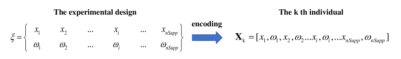
Figure 1: The $k^{th}$ individual encoding.

3.1 Repair operation

Our experience is that the current EAs are not able to find the correct number of support points in the optimal design effectively. We introduce a repair operation to tackle the issue for DE variants. In the repair process, since the true number of support points is unknown and there are usually similar support points in the generated designs, we combine the weights of similar support points as the weight for the combined point using Euclidean distance clustering. Support points with very small weights are deleted and have their weights distributed uniformly across the rest of the support points after ensuring that the sum of the weights is one. The pseudo code of the repair operation is illustrated in Algorithm 1.

Algorithm 1 The repair operation

1:$\bf{X}=min(max(\bf{X},\bf{x_{min}}),\bf{x_{max}});$

2:$index=D/nSupp:D/nSupp:D;$

3:$\bf{X}(:,index)=\bf{X}(:,index)./repmat(sum(\bf{X}(:,index),2),1,length(index));$

4:for $k=1$ to $size(\bf{X},1)$ do

5:    $Temp=reshape(\bf{X}(k,:),[\quad],nSupp);$

6:    $aux\_w=Temp(end,:)^{\prime};aux\_x=Temp(1:end-1,:)^{\prime};$

7:    $data\_not\_order=[aux\_w,aux\_x];[rows,cols]=size(data\_not\_order);$

8:    $data=sortrows(data\_not\_order,(2:cols))$;

9:    $Distance=squareform(pdist(data(:,2:size(data,2)),^{\prime}euclidean^{\prime}));$

10:    $rows=size(data,1);i=1;j=2;$

11:    while ${i<rows}$ do

12:         while ${j\leq rows}$ do

13:             if $Distance(i,j)<\epsilon$ then

14:                 $e=mean([data(i,:);data(j,:)]);e(1)=2*e(1);$

15:                 $data(j,:)=[\quad];Distance(:,j)=[\quad];rows=rows-1;$

16:                 $data(i,:)=e;$

17:             else

18:                 $j=j+1;$

19:             end if

20:         end while

21:         $i=i+1;j=i+1;$

22:         $Distance=squareform(pdist(data(:,2:size(data,2)),^{\prime}euclidean^{\prime}));$

23:    end while

24:    $condition=data(:,1)<\hat{w};data(condition,:)=[\quad];$

25:    if $size(data,1)<nSupp$ then

26:         $data=[data;repmat(zeros(1,size(data,2)),nSupp-size(data,1),1);];$

27:    end if

28:    $data=[data(:,2:end),data(:,1)];X(k,:)=reshape(data^{\prime},1,[\quad]);$

29:end for

30:$index=D/nSupp:D/nSupp:D;$

31:$\bf{X}(:,index)=\bf{X}(:,index)./repmat(sum(\bf{X}(:,index),2),1,length(index));$

3.2 DE variants

DE is a well known and widely used evolutionary metaheuristic algorithm that can search in large spaces for a solution or an approximate solution to a complex optimization problem without the use of gradient information. Like any notable metaheuristic algorithm, it has many variants which are modifications of DE in different ways for improved performance. We focus on the following seemingly more popular DE variants, such as, JADE, CoDE, SHADE, and LSHADE, and compare their abilities to search for $D$- and $A$-optimal designs for different statistical models.

JADE [20] is based on a novel greedy mutation strategy called DE/current-to-pbest/1 with the archive. The DE/current-to-pbest/1 strategy utilizes the multiple best solutions to balance the greediness of the mutation strategy and the population diversity. This archive provides information about the direction of progress and contributes to the improvement of the diversity of the population. The DE/current-to-pbest/1 strategy with the archive is as follows:

$${{\bf{v}}_{i,G}}={{\bf{x}}_{i,G}}+F\cdot({{\bf{x}}_{pbest,G}}-{{\bf{x}}_{i,G}})+F\cdot({{\bf{x}}_{{r_{1}},G}}-{{\bf{\tilde{x}}}_{{r_{2}},G}})$$ (18)

where ${{\bf{x}}_{pbest,G}}$ is randomly selected in the top of the current population with the probability ${p}$. JADE also adopts the parameter adaptation to generate the scaling factors and crossover probabilities based on the success record. During such an update, ${F}$ and ${Cr}$ values have been produced by successful offspring in recent generations. The pseudocode of JADE is illustrated in the Algorithm 2.

Algorithm 2 JADE[20]

1:Set the initial generation ${G}=0$, ${\mu_{F}=0.5}$, ${\mu_{CR}=0.5}$, ${A=\emptyset}$;

2:Step 1: The initialization operation

3:Randomly initialize the population;

4:while the stopping condition is not satisfied do

5:    ${S_{F}=\emptyset}$; ${S_{CR}=\emptyset}$;

6:    for $i=1$ to $NP$ do

7:         $F_{i}=randc_{i}(\mu_{F},0.1);$ $CR_{i}=randn_{i}(\mu_{CR},0.1);$

8:         Step 2: The “DE/current-to-pbest/1” mutation with the archive operation

9:         ${{\bf{v}}_{i,G}}={{\bf{x}}_{i,G}}+F\cdot({{\bf{x}}_{pbest,G}}-{{\bf{x}}_{i,G}})+F\cdot({{\bf{x}}_{{r_{1}},G}}-{{\bf{\tilde{x}}}_{{r_{2}},G}})$;

10:         Step 3: The binomial crossover operation

11:         for $j=1$ to $D$ do

12:             if ${\left({rand_{i,j}(0,1)\leq CR}\right){\rm{or}}\left({{j_{rand}}==j}\right)}$ then

13:                 ${{\bf{u}}_{i,G}^{j}={\bf{v}}_{i,G}^{j}}$;

14:             else

15:                 ${{\bf{u}}_{i,G}^{j}={\bf{x}}_{i,G}^{j}}$;

16:             end if

17:         end for

18:         Step 4: The selection operation

19:         if $f({{\bf{u}}_{i,G}})\leq f({{\bf{x}}_{i,G}})$ then

20:             ${{\bf{x}}_{i,G+1}={\bf{u}}_{i,G}};{{A}\longleftarrow{{\bf{x}}_{i,G}}};S_{F}\longleftarrow{F_{i}};S_{CR}\longleftarrow{CR_{i}};$

21:         end if

22:    end for

23:    Randomly remove solutions of the archive $||A||>NP$;

24:    ${\mu_{F}=(1-c)\cdot\mu_{F}+c\cdot mean_{L}(S_{F})}$; ${\mu_{CR}=(1-c)\cdot\mu_{CR}+c\cdot mean_{A}(S_{CR})}$;

25:    ${G=G+1}$;

26:end while

The composite DE (CoDE) ([21]) is proposed to generate trial vectors by different DE mutation strategies and the control parameter pool. The CoDE utilizes three mutation strategies (DE/rand/1, DE/rand/2, and DE/current-to-rand/1) and the control parameter pool is $[F=1.0,CR=0.1],[F=1.0,CR=0.9],$ and $[F=0.8,CR=0.2]$. Three candidates are generated for each trial vector by using an independent strategy, which uses a set of control parameters that are randomly selected for each trial vector. The final trial vector is chosen from the candidate with the best fitness value. The rand/1 and rand/2 strategy can generate the population to enhance the diversity in the random direction, and the current-to rand/1 strategy utilizes the rotation-invariant arithmetic crossover strategy suitable for the rotation problem. The various control parameters balance the global exploration and exploitation in the search space and Algorithm 3 is a pseudo code of CoDE.

Algorithm 3 The composite DE (CoDE) [21]

1:Set the initial generation ${G}=0$, the parameter pool:$[F=1.0,CR=0.1],[F=1.0,CR=0.9],$ and $[F=0.8,CR=0.2]$;

2:Randomly initialize the population;

3:while $FES<MaxFEs$ do

4:    for $i=1$ to $NP$ do

5:         Utilize three mutation strategies “rand/1/bin”,“rand/2/bin”, “current-to-rand/1/bin” to generate the trial vectors ${{\bf{u}}_{i_{1},G}}$, ${{\bf{u}}_{i_{2},G}}$, and ${{\bf{u}}_{i_{3},G}}$;

6:         Choose the best trial vector ${{\bf{u}}_{i,G}^{*}}$ from three trial vectors ${{\bf{u}}_{i_{1},G}}$, ${{\bf{u}}_{i_{2},G}}$, and ${{\bf{u}}_{i_{3},G}}$;

7:         if $f({{\bf{u}}_{i,G}^{*}})\leq f({{\bf{x}}_{i,G}})$ then

8:             ${{\bf{x}}_{i,G+1}={\bf{u}}_{i,G}^{*}}$;

9:         end if

10:         ${FES=FES+3}$;

11:    end for

12:    ${G=G+1}$;

13:end while

SHADE [22] adopts the different parameter mechanism based on the successful parameter historical record. SHADE calculates the history memory parameter content ${M_{F}}$ and ${M_{CR}}$ using the weighted Lehmer mean to generate the parameter ${F}$ and ${CR}$ adaptively. Algorithm 4 is our pseudo code for SHADE. In LSHADE [23], the linear population size reduction strategy is utilized to improve performance and the population size is dynamically reduced by the linear function. In the early search phase, the emphasis is on exploration and at the end of the search process, a smaller population is used to exploit the best regions. Algorithm 5 is our pseudo code for LSHADE.

Algorithm 4 SHADE [22]

1:Set the initial generation ${G}=0$, ${M_{F}=0.5}$, ${M_{CR}=0.5}$, ${A=\emptyset}$;

2:Randomly initialize the population;

3:Index counter k=1;

4:while the stopping condition is not satisfied do

5:    ${S_{F}=\emptyset}$; ${S_{CR}=\emptyset}$;

6:    for $i=1$ to $NP$ do

7:         $r_{i}$=Select from [1,H] randomly;

8:         $F_{i,G}=randc_{i}(M_{F,r_{i}},0.1);$ $CR_{i,G}=randn_{i}(M_{CR,r_{i}},0.1);$

9:         ${{\bf{v}}_{i,G}}={{\bf{x}}_{i,G}}+F_{i,G}\cdot({{\bf{x}}_{pbest,G}}-{{\bf{x}}_{i,G}})+F_{i,G}\cdot({{\bf{x}}_{{r_{1}},G}}-{{\bf{\tilde{x}}}_{{r_{2}},G}})$;

10:         for $j=1$ to $D$ do

11:             if ${\left({rand_{i,j}(0,1)\leq CR}\right){\rm{or}}\left({{j_{rand}}==j}\right)}$ then

12:                 ${{\bf{u}}_{i,G}^{j}={\bf{v}}_{i,G}^{j}}$;

13:             else

14:                 ${{\bf{u}}_{i,G}^{j}={\bf{x}}_{i,G}^{j}}$;

15:             end if

16:         end for

17:         if $f({{\bf{u}}_{i,G}})\leq f({{\bf{x}}_{i,G}})$ then

18:             ${{\bf{x}}_{i,G+1}={\bf{u}}_{i,G}};{{A}\longleftarrow{{\bf{x}}_{i,G}}};S_{F}\longleftarrow{F_{i,G}};S_{CR}\longleftarrow{CR_{i,G}};$

19:         end if

20:    end for

21:    Randomly remove solutions of the archive $\|A\|>NP$;

22:    if $S_{F}\neq\emptyset$ and $S_{CR}\neq\emptyset$ then

23:         Update ${M_{CR,k}}$, ${M_{F,k}}$ based on ${S_{CR}}$, ${S_{F}}$;

24:         $k++$;

25:         if $k>H$ then

26:             $k=1$;

27:         end if

28:    end if

29:    ${G=G+1}$;

30:end while

Algorithm 5 LSHADE [23]

1:Set the initial generation ${G}=0$, ${M_{F}=0.5}$, ${M_{CR}=0.5}$, ${A=\emptyset}$, Index counter k=1;

2:Randomly initialize the population;

3:while the stopping condition is not satisfied do

4:    ${S_{F}=\emptyset}$; ${S_{CR}=\emptyset}$;

5:    for $i=1$ to $NP$ do

6:         $r_{i}$=Select from [1,H] randomly;

7:         $F_{i,G}=randc_{i}(M_{F,r_{i}},0.1);$ If $M_{CR,r_{i}}=\perp,$ $CR_{i,G}=0.$ Else $CR_{i,G}=randn_{i}(M_{CR,r_{i}},0.1);$

8:         ${{\bf{v}}_{i,G}}={{\bf{x}}_{i,G}}+F_{i,G}\cdot({{\bf{x}}_{pbest,G}}-{{\bf{x}}_{i,G}})+F_{i,G}\cdot({{\bf{x}}_{{r_{1}},G}}-{{\bf{\tilde{x}}}_{{r_{2}},G}})$;

9:         for $j=1$ to $D$ do

10:             if ${\left({rand_{i,j}(0,1)\leq CR}\right){\rm{or}}\left({{j_{rand}}==j}\right)}$ then

11:                 ${{\bf{u}}_{i,G}^{j}={\bf{v}}_{i,G}^{j}}$;

12:             else

13:                 ${{\bf{u}}_{i,G}^{j}={\bf{x}}_{i,G}^{j}}$;

14:             end if

15:         end for

16:         if $f({{\bf{u}}_{i,G}})\leq f({{\bf{x}}_{i,G}})$ then

17:             ${{\bf{x}}_{i,G+1}={\bf{u}}_{i,G}};{{A}\longleftarrow{{\bf{x}}_{i,G}}};S_{F}\longleftarrow{F_{i,G}};S_{CR}\longleftarrow{CR_{i,G}};$

18:         end if

19:    end for

20:    Randomly remove solutions of the archive $A>NP$;

21:    if $S_{F}\neq\emptyset$ and $S_{CR}\neq\emptyset$ then

22:         Update ${M_{CR,k}}$, ${M_{F,k}}$ based on ${S_{CR}}$, ${S_{F}}$;

23:         $k++$;

24:         if $k>H$ then

25:             $k=1$;

26:         end if

27:    end if

28:    ${NP_{G+1}}=round[(\frac{{{NP^{\min}}-{NP^{init}}}}{{MaxFES}})\cdot FES+{NP^{init}}]$;

29:    if $NP_{G}<NP_{G+1}$ then

30:         Sort individuals in the population on the their fitness values and delete lowest ${NP_{G}}-{NP_{G+1}}$ individuals, and resize archive size ${A}$ according to new population;

31:    end if

32:    ${G=G+1}$;

33:end while

4 Experimental Results

In this section, we conduct experiments to find the $D$- and $A$-optimal design experiment for 12 statistical problems in [11]. In Table 1, the usefulness of these models is described in the accompanying paper cited. Problems 1 and 4 are exponential models that can be written as a sum of two exponential terms [28, 29]. The problems 2 and 8 combine the linear term with the interaction terms [30, 31] and Problem 5 is for a Kinetics of the catalytic dehydrogenation of n-hexil alcohol model [32]. Problem 6 is the Michaelis-Menten model [33] and Problem 7 concerns a mixture-type inhibition model [34]. Problems 9-11 are for the probit regression model, logistic regression model, gamma regression model, respectively and Problems 3 and 12 are the multinomial logistic regression models with different number of factors [30, 11]. Our goal is to apply the various algorithms to find $D$- and $A$-optimal designs for these models. This means we first determine the number of support points in the optimal design, where they are in the design space and the proportion of observations to take at each of the design points.

In the subsection, we apply several algorithms and compare their performance to find $D$- and $A$-optimal designs for 12 different types of models. They include traditional metaheuristic algorithms like Simulating Annealing (SA), Standard Particle Swarm Optimization (SPSO) [35], Genetic Algorithm (GA), Optimal foraging algorithm (OFA) [36] and Competitive Swarm Optimizer (CSO) [37]. Additionally, we include DE variants, which are various modifications of differential evolution, a widely used evolutionary algorithm and the variants of interest are JADE, CoDE, SHADE, and LSHADE to find the $D$-optimal and $A$-optimal design for the 12 statistical models. In the experimental setting, the population size is 50, the function evaluations (FES) of Problem 1-7 are 10000, and the function evaluations of Problem 8-12 are 500000. Each algorithm runs 25 times on each problem independently.

Table 1: Design Problems 1-12 for Various Statistical Models, along with their sources in square parentheses.

Problem	Model	Factors	Parameters	Assumed number of Support points	Variables
1 [28]	${\begin{array}[]{l}Y{\rm{\sim}}{\theta_{1}}{e^{{\rm{-}}{\theta_{2}}x}}+{\theta_{3}}{e^{{\rm{-}}{\theta_{4}}x}}+N\left({0,{\sigma^{2}}}\right),x\in\left[{0,3}\right]\\ g(\theta)=\theta\\ \text{\rm{nominal values }}\theta{\rm{=}}{\left({{\rm{1,1,1,2}}}\right)^{T}}\end{array}}$	1	4	6	12
2 [30]	$\begin{array}[]{l}Y{\rm{\sim}}{\theta_{1}}+{\theta_{2}}{x_{1}}+{\theta_{3}}x_{1}^{2}+{\theta_{4}}{x_{2}}+{\theta_{5}}{x_{1}}{x_{2}}+N\left({0,{\sigma^{2}}}\right),\\ \left({{x_{1}},{x_{2}}}\right)\in\left[{-1,1}\right]\times\left[{0,1}\right]\\ g(\theta)=\theta\end{array}$	2	5	10	30
3 [30]	$\begin{aligned} &Y\sim\pi_{i}(\mathbf{x})=P\left(Y_{i}=1\mid\mathbf{x}\right)=\frac{e^{h(\mathbf{x})^{T}\theta_{i}}}{1+e^{h(\mathbf{x})^{T}\theta_{1}+e^{h(\mathbf{x})^{T}\theta_{2}}}}\\ &\mathbf{x}\in[0,6]^{3},i=1,2\\ &h(\mathbf{x})=\left[1,\mathbf{x}^{T}\right]^{T};g(\theta)=\theta\\ &\text{ nominal values }\theta_{1}=(1,1,-1,2)^{T};\theta_{2}=(-1,2,1,-1)^{T}\end{aligned}$	3	8	15	60
4 [29]	$\begin{array}[]{l}Y{\rm{\sim}}{\theta_{1}}{e^{{\theta_{2}}x}}+{\theta_{3}}{e^{{\theta_{4}}x}}+N\left({0,{\sigma^{2}}}\right),\\ x\in\left[{0,{\rm{1}}}\right]\\ g(\theta)=\theta\\ \text{\rm{nominal values }}\theta{\rm{=}}{\left({{\rm{1,0}}{\rm{.5,1,1}}}\right)^{T}}\end{array}$	1	4	8	16
5 [32]	$\begin{array}[]{l}Y{\rm{\sim}}\frac{{{\theta_{1}}{\theta_{3}}{x_{1}}}}{{1+{\theta_{1}}{x_{1}}+{\theta_{2}}{x_{2}}}}+N\left({0,{\sigma^{2}}}\right),\\ \left({{x_{1}},{x_{2}}}\right)\in\left[{0,3}\right]\times\left[{0,3}\right]\\ g(\theta)=\theta\\ \text{\rm{nominal values }}\theta={(2.9,12.2,0.69)^{T}}\end{array}$	2	3	10	30
6 [33]	$\begin{array}[]{l}Y{\rm{\sim}}\frac{{{\theta_{1}}x}}{{{\theta_{2}}+x}}+N\left({0,{\sigma^{2}}}\right),\\ x\in\left[{0,5}\right]\\ g(\theta)=\theta\\ \text{\rm{nominal values }}\theta={(1,1)^{T}}\end{array}$	1	2	5	10
7 [34]	$\begin{array}[]{l}Y{\rm{\sim}}\frac{{{\theta_{1}}{x_{1}}}}{{\left({1+\frac{{{x_{2}}}}{{{\theta_{3}}}}}\right){\theta_{2}}+\left({1+\frac{{{x_{2}}}}{{{\theta_{4}}}}}\right){x_{1}}}}+N\left({0,{\sigma^{2}}}\right),\\ \left({{x_{1}},{x_{2}}}\right)\in\left[{0,30}\right]\times\left[{0,60}\right]\\ g(\theta)=\theta\\ \text{\rm{nominal values }}\theta={(1,4,2,4)^{T}}\end{array}$	2	4	5	15
8 [31]	$\begin{array}[]{l}Y{\rm{\sim}}{\theta_{1}}{x_{1}}+{\theta_{2}}{x_{2}}+{\theta_{3}}{x_{3}}+{\theta_{4}}{x_{1}}{x_{2}}+{\theta_{5}}{x_{1}}{x_{3}}+{\theta_{6}}{x_{2}}{x_{3}}\\ +\frac{{{\theta_{7}}}}{{{x_{1}}}}+\frac{{{\theta_{8}}}}{{{x_{2}}}}+\frac{{{\theta_{9}}}}{{{x_{3}}}}+N\left({0,{\sigma^{2}}}\right),\\ \left({{x_{1}},{x_{2}},{x_{3}}}\right)\in\left[{0.5,2}\right]\times\left[{0.5,2}\right]\times\left[{0.5,2}\right]\\ g(\theta)=\theta\end{array}$	3	9	20	80
9 [11]	$\begin{array}[]{l}Y{\rm{\sim Binomial}}\left({1,\mu}\right);\mu=\Phi(h{(x)^{T}}\theta)\\ \text{$\Phi(\cdot)${\rm{is the normal cumulative distribution function}}}\\ h(x)={[1,{x^{T}}]^{T}};x\in{\left[{-2,2}\right]^{5}}\\ g(\theta)=\theta\\ \text{\rm{nominal values }}\theta={(0.5,0.7,0.18,-0.20,-0.58,0.51)^{T}}\end{array}$	5	6	25	150
10 [11]	$\begin{array}[]{l}Y{\rm{\sim Binomial}}\left({1,\mu}\right);\mu=\frac{1}{{1+{e^{-h{{(x)}^{T}}\theta}}}}\\ h(x)={[1,{x^{T}}]^{T}};x\in{\left[{-2,2}\right]^{5}}\\ g(\theta)=\theta\\ \text{\rm{nominal values }}\theta={(0.5,0.7,0.18,-0.20,-0.58,0.51)^{T}}\end{array}$	5	6	25	150
11 [11]	$\begin{array}[]{l}Y{\rm{\sim}}\Gamma\left({1,\mu}\right);\mu={\left({{\theta_{1}}{x_{1}}+\sum\nolimits_{i=2}^{5}{{x_{i-1}}{x_{i}}{\theta_{i}}}}\right)^{2}}\\ x\in{\left[{0,10}\right]^{5}}\\ g(\theta)=\theta\\ \text{\rm{nominal values }}\theta={(0.25,0.5,0.20,0.58,0.51)^{T}}\end{array}$	5	5	25	150
12 [11]	$\begin{aligned} &Y\sim\pi_{i}(\mathbf{x})=P\left(Y_{i}=1\mid\mathbf{x}\right)=\frac{e^{h(\mathbf{x})^{T}\theta_{i}}}{1+e^{h(\mathbf{x})^{T}\theta_{1}+e^{h(\mathbf{x})^{T}\theta_{2}}}}\\ &\mathbf{x}\in[0,3]^{10},i=1,2\\ &h(\mathbf{x})=\left[1,\mathbf{x}^{T}\right]^{T};g(\theta)=\theta\\ &\text{ nominal values }\\ &\theta_{1}=(1,1,-1,2,-2,1,0.5,-0.25,0.5,-0.75,2)^{T};\\ &\theta_{2}=(-1,2,1,-1,-1,-1,-0.5,1,0.75,0.25,-2)^{T}\end{aligned}$	10	22	17	187

4.1 Algorithm-generated designs under the $D$-optimality criterion

Tables 2, 3, and 4 show the summary statistics for $D$-optimality criterion values of designs generated by different algorithms for 1-12 models. The corresponding columns show the best, median, worst, and mean objective function value on the $D$-optimal design criterion and the last two columns represent the standard derivation of each algorithm and the average Computation time in seconds. From the summary tables, we observe that LSHADE outperforms the other algorithms for the problems 2, 3, 5, 7, and 12 in terms of median value. SHADE also achieves better performance on the problems 8-10 and JADE obtains better result on problem 11 in terms of the median value. Compared with CSO, LSHADE obtains the inferior results on the problems 4 and 6, and outperforms on the rest problems. Overall the DE variants outperform OFA and the traditional EA such as the SA, SPSO, GA.

Table 2: Summary statistics for $D$-optimality criterion values of designs generated by different algorithms for 1-4 models.

Problem	Algorithm	best	median	worst	mean	std	time
1	SA	2.0950E+01	2.1369E+01	2.1931E+01	2.1441E+01	2.9427E-01	5.3642E+00
	SPSO	2.0517E+01	2.0585E+01	2.0654E+01	2.0587E+01	3.7838E-02	6.1441E+00
	GA	2.0525E+01	2.0558E+01	2.0602E+01	2.0556E+01	2.0318E-02	4.2281E+00
	OFA	2.0523E+01	2.0573E+01	2.0653E+01	2.0575E+01	3.1526E-02	3.7729E+00
	CSO	2.0508E+01	2.0508E+01	2.0517E+01	2.0509E+01	1.6465E-03	3.8454E+00
	JADE	2.0508E+01	2.0508E+01	2.0508E+01	2.0508E+01	6.8025E-10	3.9214E+00
	CoDE	2.0508E+01	2.0509E+01	2.0511E+01	2.0509E+01	4.7857E-04	4.3009E+00
	SHADE	2.0508E+01	2.0508E+01	2.0508E+01	2.0508E+01	1.2866E-08	4.5524E+00
	LSHADE	2.0508E+01	2.0508E+01	2.0508E+01	2.0508E+01	1.8354E-05	6.0343E+00
2	SA	5.6730E+00	6.0433E+00	7.5963E+00	6.1876E+00	4.9394E-01	8.2503E+00
	SPSO	5.6155E+00	6.0435E+00	6.4494E+00	6.0886E+00	2.2373E-01	9.3157E+00
	GA	6.1859E+00	6.5607E+00	7.0657E+00	6.6318E+00	2.2003E-01	6.9724E+00
	OFA	5.4921E+00	6.0236E+00	6.6990E+00	6.0876E+00	3.3401E-01	8.0033E+00
	CSO	5.0443E+00	5.2064E+00	5.5156E+00	5.2167E+00	1.1736E-01	5.5990E+00
	JADE	5.0811E+00	5.1441E+00	5.2143E+00	5.1506E+00	3.4243E-02	6.6867E+00
	CoDE	5.4858E+00	5.7458E+00	5.9051E+00	5.7220E+00	1.2025E-01	7.4948E+00
	SHADE	5.1742E+00	5.2753E+00	5.3571E+00	5.2672E+00	5.0745E-02	8.1721E+00
	LSHADE	5.0219E+00	5.0227E+00	5.2656E+00	5.0501E+00	5.6540E-02	8.2123E+00
3	SA	1.9539E+01	2.1143E+01	2.4438E+01	2.1250E+01	1.2990E+00	1.7355E+01
	SPSO	1.8433E+01	1.9642E+01	2.0614E+01	1.9708E+01	5.3792E-01	2.0101E+01
	GA	1.9198E+01	2.0144E+01	2.1234E+01	2.0149E+01	5.7839E-01	1.7473E+01
	OFA	1.9602E+01	2.0752E+01	2.1667E+01	2.0770E+01	5.0845E-01	1.9847E+01
	CSO	1.6691E+01	1.7707E+01	1.8682E+01	1.7761E+01	5.0523E-01	1.4178E+01
	JADE	1.7409E+01	1.7880E+01	1.8385E+01	1.7871E+01	2.8381E-01	1.7929E+01
	CoDE	1.8320E+01	1.9258E+01	1.9684E+01	1.9112E+01	3.8079E-01	1.6960E+01
	SHADE	1.7304E+01	1.8248E+01	1.8757E+01	1.8227E+01	2.8792E-01	2.1254E+01
	LSHADE	1.6121E+01	1.6283E+01	1.6695E+01	1.6360E+01	1.6745E-01	2.8408E+01
4	SA	2.2182E+01	2.2629E+01	2.3160E+01	2.2641E+01	2.5755E-01	5.6349E+00
	SPSO	2.1027E+01	2.1111E+01	2.1228E+01	2.1112E+01	5.5062E-02	6.2601E+00
	GA	2.1053E+01	2.1133E+01	2.1254E+01	2.1144E+01	5.4330E-02	4.6637E+00
	OFA	2.1041E+01	2.1085E+01	2.1188E+01	2.1101E+01	4.4650E-02	4.3282E+00
	CSO	2.1022E+01	2.1022E+01	2.1022E+01	2.1022E+01	1.1110E-06	4.0850E+00
	JADE	2.1022E+01	2.1022E+01	2.1022E+01	2.1022E+01	1.0122E-09	4.1126E+00
	CoDE	2.1022E+01	2.1023E+01	2.1023E+01	2.1023E+01	6.5874E-05	4.2364E+00
	SHADE	2.1022E+01	2.1022E+01	2.1022E+01	2.1022E+01	1.3467E-09	4.8679E+00
	LSHADE	2.1022E+01	2.1022E+01	2.1029E+01	2.1023E+01	1.2089E-03	6.1771E+00

Table 3: Summary statistics for $D$-optimality criterion values of designs generated by different algorithms for 5-8 models.

Problem	Algorithm	best	median	worst	mean	std	time
5	SA	1.9014E+01	1.9829E+01	2.0649E+01	1.9837E+01	4.4351E-01	1.0149E+01
	SPSO	1.8559E+01	1.8834E+01	1.9201E+01	1.8839E+01	1.6180E-01	1.0475E+01
	GA	1.8521E+01	1.8759E+01	1.8915E+01	1.8744E+01	1.0214E-01	8.4169E+00
	OFA	1.8715E+01	1.9061E+01	1.9503E+01	1.9085E+01	2.1220E-01	9.3761E+00
	CSO	1.8328E+01	1.8335E+01	1.8388E+01	1.8341E+01	1.5112E-02	5.8712E+00
	JADE	1.8340E+01	1.8351E+01	1.8369E+01	1.8352E+01	8.6070E-03	8.3880E+00
	CoDE	1.8563E+01	1.8660E+01	1.8779E+01	1.8664E+01	6.0923E-02	9.1251E+00
	SHADE	1.8338E+01	1.8371E+01	1.8412E+01	1.8373E+01	1.8124E-02	9.6797E+00
	LSHADE	1.8328E+01	1.8328E+01	1.8330E+01	1.8328E+01	4.3515E-04	9.0270E+00
6	SA	5.2563E+00	5.3232E+00	5.6250E+00	5.3571E+00	1.1280E-01	4.6965E+00
	SPSO	5.2529E+00	5.2556E+00	5.2700E+00	5.2566E+00	4.1190E-03	5.0812E+00
	GA	5.2563E+00	5.2618E+00	5.2690E+00	5.2616E+00	4.0658E-03	3.7057E+00
	OFA	5.2532E+00	5.2568E+00	5.2734E+00	5.2579E+00	4.8636E-03	3.4635E+00
	CSO	5.2528E+00	5.2528E+00	5.2528E+00	5.2528E+00	3.1869E-15	3.0429E+00
	JADE	5.2528E+00	5.2528E+00	5.2528E+00	5.2528E+00	4.9944E-11	3.4204E+00
	CoDE	5.2528E+00	5.2529E+00	5.2543E+00	5.2530E+00	3.2672E-04	3.6795E+00
	SHADE	5.2528E+00	5.2528E+00	5.2528E+00	5.2528E+00	4.0355E-12	4.2826E+00
	LSHADE	5.2528E+00	5.2528E+00	5.2529E+00	5.2528E+00	1.1133E-05	4.9213E+00
7	SA	2.5206E+01	2.6849E+01	2.9695E+01	2.7104E+01	1.3432E+00	6.4176E+00
	SPSO	2.5987E+01	2.8507E+01	2.9983E+01	2.8335E+01	1.0567E+00	5.6918E+00
	GA	2.5222E+01	2.5731E+01	2.6698E+01	2.5743E+01	3.2034E-01	4.6229E+00
	OFA	2.5584E+01	2.6437E+01	2.7540E+01	2.6424E+01	4.8131E-01	4.1098E+00
	CSO	2.4755E+01	2.4817E+01	2.5076E+01	2.4840E+01	9.0283E-02	4.4402E+00
	JADE	2.4755E+01	2.4764E+01	2.4786E+01	2.4765E+01	6.8432E-03	4.8036E+00
	CoDE	2.4970E+01	2.5145E+01	2.5401E+01	2.5164E+01	1.1437E-01	4.8842E+00
	SHADE	2.4764E+01	2.4773E+01	2.4812E+01	2.4778E+01	1.4106E-02	5.5157E+00
	LSHADE	2.4752E+01	2.4752E+01	2.4946E+01	2.4760E+01	3.8811E-02	7.3086E+00
8	SA	1.7440E+01	1.9019E+01	1.9510E+01	1.9084E+01	4.0072E-01	8.0268E+02
	SPSO	1.3380E+01	1.4211E+01	1.4912E+01	1.4213E+01	3.5979E-01	7.8987E+02
	GA	1.9646E+01	2.1166E+01	2.2210E+01	2.0989E+01	7.1101E-01	6.2538E+02
	OFA	1.3687E+01	1.4605E+01	1.5296E+01	1.4534E+01	4.5288E-01	5.4602E+02
	CSO	1.3079E+01	1.5750E+01	1.7425E+01	1.5572E+01	1.0201E+00	6.2543E+02
	JADE	1.0123E+01	1.0137E+01	1.0188E+01	1.0140E+01	1.4061E-02	7.3665E+02
	CoDE	1.1238E+01	1.1481E+01	1.1660E+01	1.1477E+01	1.0074E-01	6.7893E+02
	SHADE	1.0120E+01	1.0132E+01	1.0151E+01	1.0131E+01	7.2142E-03	8.3684E+02
	LSHADE	1.0141E+01	1.0355E+01	1.7984E+01	1.1012E+01	1.6465E+00	8.5980E+02

Table 4: Summary statistics for $D$-optimality criterion values of designs generated by different algorithms for 9-12 models.

Problem	Algorithm	best	median	worst	mean	std	time
9	SA	2.1138E+00	3.5850E+00	5.5857E+00	3.6311E+00	8.0692E-01	1.7705E+03
	SPSO	1.9491E+00	2.2749E+00	2.7721E+00	2.2755E+00	1.6800E-01	2.1851E+03
	GA	2.3355E+00	2.7209E+00	2.8683E+00	2.6935E+00	1.4640E-01	2.0297E+03
	OFA	-4.7730E-01	-1.4708E-01	6.3570E-01	-4.7291E-02	3.2590E-01	1.4896E+03
	CSO	-1.0171E+00	-5.0889E-01	1.0382E-01	-4.5812E-01	3.2599E-01	1.5052E+03
	JADE	-1.4051E+00	-1.3942E+00	-1.3722E+00	-1.3935E+00	7.2466E-03	1.6989E+03
	CoDE	-9.5511E-01	-6.2197E-01	-3.3163E-01	-5.9983E-01	1.4441E-01	1.5607E+03
	SHADE	-1.4058E+00	-1.3957E+00	-1.3645E+00	-1.3946E+00	9.4775E-03	1.2752E+03
	LSHADE	-1.4099E+00	-1.3803E+00	-1.3335E+00	-1.3788E+00	1.7491E-02	1.4326E+03
10	SA	9.6203E+00	1.1093E+01	1.3250E+01	1.1146E+01	1.0032E+00	8.1256E+02
	SPSO	6.8778E+00	7.3106E+00	7.6479E+00	7.3302E+00	1.8711E-01	1.2783E+03
	GA	7.3239E+00	7.7247E+00	7.9990E+00	7.6912E+00	1.6754E-01	1.1488E+03
	OFA	5.3458E+00	6.4498E+00	6.7960E+00	6.3674E+00	3.9753E-01	7.9646E+02
	CSO	4.1360E+00	4.6397E+00	5.2884E+00	4.6058E+00	3.2267E-01	6.5452E+02
	JADE	3.7108E+00	3.7162E+00	3.7363E+00	3.7198E+00	8.9034E-03	8.5128E+02
	CoDE	4.3516E+00	4.5441E+00	4.7225E+00	4.5422E+00	8.5509E-02	7.9899E+02
	SHADE	3.7092E+00	3.7161E+00	3.7288E+00	3.7173E+00	4.3694E-03	8.3846E+02
	LSHADE	3.7087E+00	3.7354E+00	3.9989E+00	3.7526E+00	5.6766E-02	8.9841E+02
11	SA	-1.9743E+00	-1.8435E+00	1.2587E+01	3.3043E+00	7.1055E+00	1.0568E+03
	SPSO	-5.1770E+00	-3.5075E+00	-1.5682E+00	-3.5155E+00	9.5282E-01	1.1954E+03
	GA	-4.9769E+00	-1.1644E+00	7.3234E-01	-1.2660E+00	1.2505E+00	1.0956E+03
	OFA	-7.2037E+00	-6.7809E+00	-5.9558E+00	-6.7419E+00	3.0416E-01	9.3847E+02
	CSO	-7.1550E+00	-6.2678E+00	-5.6565E+00	-6.3541E+00	4.6642E-01	1.0135E+03
	JADE	-8.6005E+00	-8.6003E+00	-8.6001E+00	-8.6003E+00	1.1716E-04	1.0640E+03
	CoDE	-7.9452E+00	-7.8098E+00	-7.6923E+00	-7.8139E+00	7.0938E-02	8.8282E+02
	SHADE	-8.5980E+00	-8.5944E+00	-8.5902E+00	-8.5945E+00	2.0392E-03	1.0306E+03
	LSHADE	-8.5987E+00	-8.5795E+00	-5.3369E+00	-8.0841E+00	8.8577E-01	1.0936E+03
12	SA	9.1286E+01	1.0172E+02	1.1639E+02	1.0205E+02	6.2509E+00	1.0663E+03
	SPSO	7.0244E+01	7.3279E+01	7.5312E+01	7.3122E+01	1.2190E+00	1.2432E+03
	GA	6.9499E+01	7.3638E+01	7.6067E+01	7.3484E+01	1.6996E+00	1.0153E+03
	OFA	6.0067E+01	6.4620E+01	6.6220E+01	6.4273E+01	1.6884E+00	8.4061E+02
	CSO	4.9104E+01	5.6595E+01	6.7650E+01	5.7496E+01	4.4471E+00	8.6097E+02
	JADE	3.5215E+01	3.5923E+01	3.6730E+01	3.5914E+01	3.2457E-01	1.0156E+03
	CoDE	3.9260E+01	4.4461E+01	4.8282E+01	4.4077E+01	2.5368E+00	1.0337E+03
	SHADE	3.4703E+01	3.5327E+01	3.6080E+01	3.5334E+01	3.0471E-01	9.8981E+02
	LSHADE	3.3481E+01	3.4330E+01	4.8622E+01	3.4906E+01	2.8913E+00	9.9196E+02

In Table 5, the Wilcoxon rank test was applied to test equality of the $D$-optimal design criterion values from various algorithms at the 0.05 significance level. The notations ‘-’, ‘+’, and ‘=’ indicate that the corresponding comparative algorithm in the column of table is significantly worse than, better than, or similar to the criterion value of the target algorithm shown in the row of the table, respectively. Table 5 shows that LSHADE outperforms other comparative algorithms and the OFA and the traditional evolutionary algorithms(SA, SPSO, and GA) are inferior to DE variants such as JADE, CoDE, SHADE, and LSHADE. CSO is also a competitive algorithm better than CoDE, OFA, and the traditional EAs, but inferior to JADE, SHADE, and LSHADE.

Table 5: Results of the Wilcoxon rank tests for the equality of the medians of values of the $D$-optimality criterion values of designs generated from various algorithms at the 0.05 significance level.

-/+/=	SA	SPSO	GA	OFA	CSO	JADE	CoDE	SHADE	LSHADE
SA	[0/0/12]	[10/1/1]	[9/2/1]	[9/0/3]	[12/0/0]	[12/0/0]	[12/0/0]	[12/0/0]	[12/0/0]
SPSO	[1/10/1]	[0/0/12]	[2/7/3]	[5/3/4]	[11/1/0]	[12/0/0]	[12/0/0]	[12/0/0]	[12/0/0]
GA	[2/9/1]	[7/2/3]	[0/0/12]	[8/4/0]	[12/0/0]	[12/0/0]	[12/0/0]	[12/0/0]	[12/0/0]
OFA	[0/9/3]	[3/5/4]	[4/8/0]	[0/0/12]	[10/2/0]	[12/0/0]	[12/0/0]	[12/0/0]	[12/0/0]
CSO	[0/12/0]	[1/11/0]	[0/12/0]	[2/10/0]	[0/0/12]	[8/3/1]	[3/7/2]	[7/5/0]	[10/2/0]
JADE	[0/12/0]	[0/12/0]	[0/12/0]	[0/12/0]	[3/8/1]	[0/0/12]	[0/12/0]	[2/6/4]	[7/5/0]
CoDE	[0/12/0]	[0/12/0]	[0/12/0]	[0/12/0]	[7/3/2]	[12/0/0]	[0/0/12]	[12/0/0]	[12/0/0]
SHADE	[0/12/0]	[0/12/0]	[0/12/0]	[0/12/0]	[5/7/0]	[6/2/4]	[0/12/0]	[0/0/12]	[7/4/1]
LSHADE	[0/12/0]	[0/12/0]	[0/12/0]	[0/12/0]	[2/10/0]	[5/7/0]	[0/12/0]	[4/7/1]	[0/0/12]

Figure 2 displays the convergence rate of all algorithms for finding the $D$-optimal designs for the statistical model. The X axis represents the number of function evaluations and the Y axis represents the mean $D$-optimal design criterion values on the log scale. The LSHADE algorithm shows better convergence performance than other comparative algorithms on the Problem 1-7, 9-10 and 12. JADE and SHADE obtain the convergence on the problem 8 and 11. Overall DE variants exhibit better convergence ability.

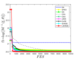
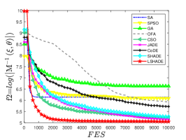
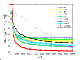
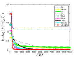
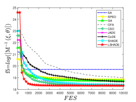
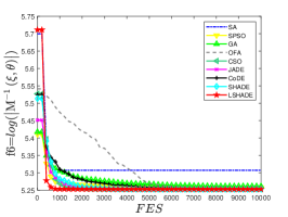
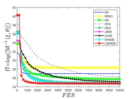
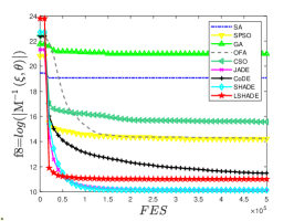
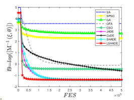
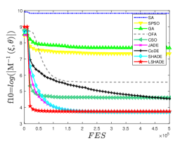
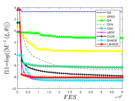
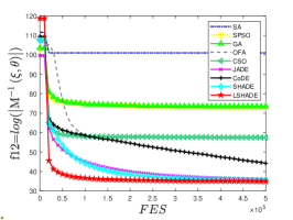
Figure 2: Mean Performance of the SA, SPSO, GA, OFA, CSO, JADE, CoDE, SHADE, and LSHADE algorithms for finding $D$-optimal designs.

4.2 Designs found by various algorithms under the $A$-optimality criterion

Tables 6, 7, and 8 show the summary statistics for $A$-optimality criterion values of designs generated by different algorithms for models 1-12, such as the best, median, worst, and median value, standard deviation, and Computation time. From tables, we can observe that LSHADE can obtain better performance on the Problems 2 , 3, 5, 7, 9, and 12 in terms of the median values. On the problems 8, 10 and 11, SHADE achieves better result in terms of the median values. Except for the Problems 8 and 10, LSHADE obtains the best performance in terms of the best values. Compared with OFA and the traditional EAs (SA, SPSO, and GA), DE variants obtain superior results.

Table 6: Summary statistics for $A$-optimality criterion values of designs generated by different algorithms for models 1-4.

Problem	Algorithm	best	median	worst	mean	std	time
1	SA	5.4106E+04	5.5325E+04	6.0497E+04	5.5603E+04	1.3189E+03	5.3486E+00
	SPSO	5.3870E+04	5.5045E+04	5.9888E+04	5.5807E+04	1.8094E+03	5.5440E+00
	GA	5.5324E+04	5.7162E+04	6.0459E+04	5.7363E+04	1.1872E+03	4.6051E+00
	OFA	5.4040E+04	5.4604E+04	5.5677E+04	5.4686E+04	4.5277E+02	3.5254E+00
	CSO	5.3797E+04	5.3797E+04	5.3800E+04	5.3797E+04	6.2337E-01	3.7374E+00
	JADE	5.3797E+04	5.3797E+04	5.3797E+04	5.3797E+04	4.9717E-04	3.8483E+00
	CoDE	5.3801E+04	5.3817E+04	5.4021E+04	5.3833E+04	4.7297E+01	4.4170E+00
	SHADE	5.3797E+04	5.3797E+04	5.3797E+04	5.3797E+04	2.1238E-04	6.0526E+00
	LSHADE	5.3797E+04	5.3797E+04	5.3806E+04	5.3797E+04	1.8110E+00	8.2115E+00
2	SA	2.2132E+01	2.4535E+01	2.5309E+01	2.4355E+01	7.6792E-01	6.2339E+00
	SPSO	2.4813E+01	2.9798E+01	3.2309E+01	2.9196E+01	2.1380E+00	8.5148E+00
	GA	2.9523E+01	3.5465E+01	3.9113E+01	3.5036E+01	2.5656E+00	6.7971E+00
	OFA	2.3854E+01	2.6579E+01	3.0040E+01	2.6834E+01	1.7220E+00	5.4673E+00
	CSO	2.1135E+01	2.2366E+01	2.5764E+01	2.2770E+01	1.4652E+00	6.1731E+00
	JADE	2.1370E+01	2.1962E+01	2.2542E+01	2.1944E+01	2.9728E-01	6.6322E+00
	CoDE	2.5084E+01	2.6758E+01	2.9199E+01	2.6879E+01	1.0002E+00	1.2787E+01
	SHADE	2.2375E+01	2.2970E+01	2.3738E+01	2.2944E+01	3.9143E-01	1.0042E+01
	LSHADE	2.0953E+01	2.0953E+01	2.1986E+01	2.1045E+01	2.5188E-01	8.4403E+00
3	SA	2.7080E+02	2.9571E+02	3.3889E+02	2.9688E+02	1.5384E+01	1.6590E+01
	SPSO	3.2764E+02	3.7085E+02	3.9487E+02	3.6773E+02	1.8336E+01	2.0000E+01
	GA	3.5742E+02	4.1121E+02	4.7246E+02	4.1178E+02	2.6043E+01	1.7498E+01
	OFA	3.7008E+02	4.3167E+02	5.5963E+02	4.3882E+02	4.2038E+01	1.3134E+01
	CSO	2.5645E+02	2.8817E+02	3.2157E+02	2.9018E+02	1.6787E+01	1.6083E+01
	JADE	2.7998E+02	2.8812E+02	2.9649E+02	2.8778E+02	4.8596E+00	1.7286E+01
	CoDE	3.0548E+02	3.4264E+02	3.8399E+02	3.4323E+02	1.5921E+01	2.2902E+01
	SHADE	2.8308E+02	2.9356E+02	3.1122E+02	2.9471E+02	7.9760E+00	2.4603E+01
	LSHADE	2.4507E+02	2.5082E+02	2.6520E+02	2.5269E+02	5.4921E+00	2.1897E+01
4	SA	9.5679E+06	1.0404E+07	1.1958E+07	1.0613E+07	6.6248E+05	5.9636E+00
	SPSO	9.4782E+06	1.0196E+07	1.1210E+07	1.0176E+07	5.0031E+05	6.2734E+00
	GA	9.6035E+06	1.0087E+07	1.0787E+07	1.0102E+07	2.8905E+05	4.6499E+00
	OFA	9.4452E+06	9.4790E+06	9.5824E+06	9.4837E+06	3.3395E+04	3.7862E+00
	CSO	9.4050E+06	9.4050E+06	9.4070E+06	9.4051E+06	4.4342E+02	4.0363E+00
	JADE	9.4050E+06	9.4050E+06	9.4050E+06	9.4050E+06	5.1666E-03	4.1759E+00
	CoDE	9.4050E+06	9.4051E+06	9.4058E+06	9.4052E+06	2.0252E+02	4.0380E+00
	SHADE	9.4050E+06	9.4050E+06	9.4050E+06	9.4050E+06	7.1280E-03	6.3865E+00
	LSHADE	9.4050E+06	9.4050E+06	9.4448E+06	9.4068E+06	7.9927E+03	6.6705E+00

Table 7: Summary statistics for $A$-optimality criterion values of designs generated by different algorithms for nodels 5-8.

Problem	Algorithm	best	median	worst	mean	std	time
5	SA	2.9758E+04	3.3929E+04	4.0145E+04	3.4326E+04	3.0119E+03	9.7461E+00
	SPSO	3.5928E+04	3.9208E+04	4.2549E+04	3.9294E+04	1.6376E+03	1.1562E+01
	GA	3.2974E+04	3.6597E+04	4.1268E+04	3.6511E+04	1.7600E+03	9.2352E+00
	OFA	3.4009E+04	3.8511E+04	4.5745E+04	3.8785E+04	2.8842E+03	8.3596E+00
	CSO	2.9262E+04	2.9707E+04	3.0658E+04	2.9853E+04	4.4212E+02	8.3292E+00
	JADE	2.9317E+04	2.9576E+04	3.0045E+04	2.9623E+04	1.9048E+02	8.6112E+00
	CoDE	3.2457E+04	3.5652E+04	3.8275E+04	3.5662E+04	1.6036E+03	1.2272E+01
	SHADE	2.9347E+04	2.9927E+04	3.0749E+04	2.9928E+04	3.7348E+02	1.3310E+01
	LSHADE	2.9159E+04	2.9159E+04	2.9230E+04	2.9163E+04	1.4794E+01	1.2400E+01
6	SA	8.0175E+01	8.0193E+01	8.0352E+01	8.0216E+01	5.4783E-02	4.6936E+00
	SPSO	8.0200E+01	8.0635E+01	8.3339E+01	8.1013E+01	8.6480E-01	5.0745E+00
	GA	8.0210E+01	8.0799E+01	8.2541E+01	8.0838E+01	4.9661E-01	3.8337E+00
	OFA	8.0176E+01	8.0216E+01	8.0523E+01	8.0256E+01	9.4868E-02	3.1545E+00
	CSO	8.0174E+01	8.0174E+01	8.0174E+01	8.0174E+01	3.4688E-14	3.0322E+00
	JADE	8.0174E+01	8.0174E+01	8.0174E+01	8.0174E+01	9.5485E-10	3.3564E+00
	CoDE	8.0174E+01	8.0181E+01	8.0228E+01	8.0186E+01	1.3382E-02	4.2377E+00
	SHADE	8.0174E+01	8.0174E+01	8.0174E+01	8.0174E+01	7.3451E-11	3.6520E+00
	LSHADE	8.0174E+01	8.0174E+01	8.0174E+01	8.0174E+01	6.0380E-07	5.5921E+00
7	SA	9.9471E+03	1.1067E+04	2.9991E+04	1.2937E+04	4.5044E+03	6.6180E+00
	SPSO	2.5409E+04	5.5562E+04	2.1145E+05	7.1136E+04	4.9829E+04	5.7289E+00
	GA	1.3296E+04	1.6761E+04	2.0522E+04	1.6604E+04	1.6807E+03	4.6489E+00
	OFA	1.3151E+04	1.7404E+04	2.7657E+04	1.8156E+04	3.6027E+03	3.8027E+00
	CSO	9.8906E+03	1.0043E+04	2.6240E+04	1.1833E+04	3.5279E+03	4.4800E+00
	JADE	9.8928E+03	9.9235E+03	9.9805E+03	9.9337E+03	2.5456E+01	4.5579E+00
	CoDE	1.1313E+04	1.3133E+04	1.4179E+04	1.2965E+04	6.8265E+02	5.9052E+00
	SHADE	9.9220E+03	9.9729E+03	1.0274E+04	1.0004E+04	8.4994E+01	5.1934E+00
	LSHADE	9.8712E+03	9.8714E+03	1.0726E+04	9.9328E+03	1.8271E+02	6.8315E+00
8	SA	2.6164E+02	3.5394E+02	1.0245E+04	1.1754E+03	2.7314E+03	7.6358E+02
	SPSO	2.0337E+02	2.4411E+02	2.6659E+02	2.4239E+02	1.7058E+01	7.7314E+02
	GA	4.4853E+02	6.7084E+02	8.4174E+02	6.7716E+02	8.5607E+01	7.1019E+02
	OFA	1.7198E+02	1.9189E+02	2.1300E+02	1.9224E+02	1.1243E+01	5.9679E+02
	CSO	1.8350E+02	2.6286E+02	3.8066E+02	2.6064E+02	4.7158E+01	6.4924E+02
	JADE	1.0702E+02	1.0723E+02	1.0746E+02	1.0723E+02	1.1690E-01	7.0780E+02
	CoDE	1.3400E+02	1.3844E+02	1.4526E+02	1.3884E+02	2.6946E+00	7.7524E+02
	SHADE	1.0684E+02	1.0700E+02	1.0711E+02	1.0700E+02	5.6425E-02	9.4994E+02
	LSHADE	1.0707E+02	1.1236E+02	9.7052E+02	2.1764E+02	2.2440E+02	1.0174E+03

Table 8: Summary statistics for $A$-optimality criterion values of designs generated by different algorithms for 9-12 models

Problem	Algorithm	best	median	worst	mean	std	time
9	SA	1.2369E+01	1.4007E+01	1.6018E+01	1.4199E+01	9.5456E-01	1.7186E+03
	SPSO	1.1587E+01	1.1994E+01	1.2593E+01	1.2042E+01	3.0643E-01	2.0798E+03
	GA	1.1821E+01	1.2866E+01	1.3311E+01	1.2818E+01	3.1679E-01	1.9393E+03
	OFA	9.3931E+00	1.0589E+01	1.0999E+01	1.0456E+01	4.0683E-01	1.5424E+03
	CSO	7.9295E+00	8.7028E+00	9.2882E+00	8.6300E+00	3.7578E-01	1.5904E+03
	JADE	7.3583E+00	7.4057E+00	7.4414E+00	7.4015E+00	1.9565E-02	1.7625E+03
	CoDE	8.0619E+00	8.3577E+00	8.5831E+00	8.3257E+00	1.5422E-01	1.8042E+03
	SHADE	7.3431E+00	7.3920E+00	7.4168E+00	7.3889E+00	2.1006E-02	2.6446E+03
	LSHADE	7.3293E+00	7.3878E+00	7.4841E+00	7.3907E+00	3.9136E-02	2.5987E+03
10	SA	2.3820E+01	2.9747E+01	4.3875E+01	3.0050E+01	3.5895E+00	8.0972E+02
	SPSO	2.3032E+01	2.5519E+01	2.6387E+01	2.5381E+01	8.9345E-01	1.2398E+03
	GA	2.5859E+01	2.7250E+01	2.8201E+01	2.7223E+01	6.6991E-01	1.1124E+03
	OFA	2.0515E+01	2.2553E+01	2.3555E+01	2.2246E+01	8.3694E-01	7.9705E+02
	CSO	1.6770E+01	1.7887E+01	1.9104E+01	1.7945E+01	6.2586E-01	6.9893E+02
	JADE	1.5769E+01	1.5812E+01	1.5863E+01	1.5814E+01	2.6860E-02	9.3603E+02
	CoDE	1.7166E+01	1.7747E+01	1.8451E+01	1.7747E+01	2.8636E-01	9.6280E+02
	SHADE	1.5751E+01	1.5798E+01	1.5837E+01	1.5798E+01	2.2046E-02	1.0642E+03
	LSHADE	1.5754E+01	1.5841E+01	1.8002E+01	1.5926E+01	4.3540E-01	1.0955E+03
11	SA	3.2939E+00	4.0178E+00	2.8862E+01	6.5907E+00	6.9270E+00	1.0999E+03
	SPSO	2.4552E+00	3.8679E+00	6.2302E+00	3.7815E+00	7.6485E-01	1.1716E+03
	GA	5.4945E+00	1.3534E+01	3.1080E+01	1.5247E+01	6.9933E+00	1.0327E+03
	OFA	1.4953E+00	1.7660E+00	2.0155E+00	1.7579E+00	1.5643E-01	6.6999E+02
	CSO	1.3351E+00	1.6648E+00	2.7873E+00	1.7952E+00	3.6727E-01	1.0173E+03
	JADE	1.0674E+00	1.0674E+00	1.0674E+00	1.0674E+00	9.4758E-06	1.0578E+03
	CoDE	1.2481E+00	1.2936E+00	1.3465E+00	1.2921E+00	2.3161E-02	1.1228E+03
	SHADE	1.0674E+00	1.0674E+00	1.0675E+00	1.0674E+00	2.5077E-05	1.0489E+03
	LSHADE	1.0674E+00	1.1116E+00	3.9579E+00	1.3923E+00	6.3747E-01	1.1310E+03
12	SA	2.2814E+03	3.4212E+03	7.3525E+03	3.5450E+03	1.0615E+03	1.1807E+03
	SPSO	2.3281E+03	2.9545E+03	3.3204E+03	2.9098E+03	2.3086E+02	1.1599E+03
	GA	2.7812E+03	4.0523E+03	4.7256E+03	3.9017E+03	5.3264E+02	1.0356E+03
	OFA	8.3454E+02	9.7932E+02	1.2060E+03	9.8595E+02	9.3728E+01	6.8357E+02
	CSO	8.1973E+02	1.2846E+03	2.6201E+03	1.3300E+03	4.0423E+02	5.3893E+02
	JADE	3.5190E+02	3.6169E+02	3.7907E+02	3.6279E+02	6.5371E+00	1.0194E+03
	CoDE	3.6852E+02	4.0345E+02	5.5261E+02	4.0886E+02	4.0404E+01	1.5123E+03
	SHADE	3.3836E+02	3.4646E+02	3.5645E+02	3.4726E+02	4.7466E+00	1.3289E+03
	LSHADE	3.0982E+02	3.1866E+02	6.4707E+02	3.3166E+02	6.5911E+01	1.2138E+03

Table 9 reports results from the Wilcoxon rank tests whether the $A$-optimal design criterion are different at the 0.05 significance level. The notations ‘-’, ‘+’, and ‘=’ indicate that the corresponding comparative algorithm in the column of table is significantly worse than, better than, and similar to the target algorithm shown in the row of the table, respectively. Table 9 shows that LSHADE outperforms than other comparative algorithms and the traditional evolutionary algorithms (SA, SPSO, and GA) and OFA are under-perform DE variants, such as JADE, CoDE, SHADE, and LSHADE. We note that CSO is also inferior to JADE, SHADE and LSHADE.

Table 9: Results of the Wilcoxon rank tests for the equality of the medians of values of the $A$-optimality criterion values of designs generated from various algorithms at the 0.05 significance level.

-/+/=	SA	SPSO	GA	OFA	CSO	JADE	CoDE	SHADE	LSHADE
SA	[0/0/12]	[6/5/1]	[3/9/0]	[7/5/0]	[11/0/1]	[12/0/0]	[8/4/0]	[11/0/1]	[12/0/0]
SPSO	[5/6/1]	[0/0/12]	[2/8/2]	[9/1/2]	[11/0/1]	[12/0/0]	[12/0/0]	[12/0/0]	[12/0/0]
GA	[9/3/0]	[8/2/2]	[0/0/12]	[9/2/1]	[12/0/0]	[12/0/0]	[11/0/1]	[12/0/0]	[12/0/0]
OFA	[5/7/0]	[1/9/2]	[2/9/1]	[0/0/12]	[9/2/1]	[12/0/0]	[11/0/1]	[12/0/0]	[12/0/0]
CSO	[0/11/1]	[0/11/1]	[0/12/0]	[2/9/1]	[0/0/12]	[6/2/4]	[4/7/1]	[5/2/5]	[9/1/2]
JADE	[0/12/0]	[0/12/0]	[0/12/0]	[0/12/0]	[2/6/4]	[0/0/12]	[0/12/0]	[2/6/4]	[6/4/2]
CoDE	[4/8/0]	[0/12/0]	[0/11/1]	[0/11/1]	[7/4/1]	[12/0/0]	[0/0/12]	[12/0/0]	[11/0/1]
SHADE	[0/11/1]	[0/12/0]	[0/12/0]	[0/12/0]	[2/5/5]	[6/2/4]	[0/12/0]	[0/0/12]	[6/4/2]
LSHADE	[0/12/0]	[0/12/0]	[0/12/0]	[0/12/0]	[1/9/2]	[4/6/2]	[0/11/1]	[4/6/2]	[0/0/12]

Figure 3 displays the convergence pattern of all algorithms. The X axial represents the number of function evaluations and the Y axial is the mean of the logarithmic $A$-optimal design criterion value. We observe that LSHADE has outstanding convergence performance for Problems 1-7, 9-10 and 12, while JADE and SHADE have better convergence characteristics for the Problems 8 and 11.

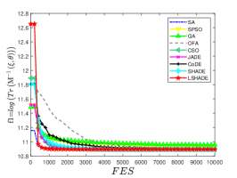
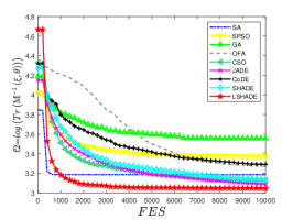
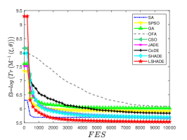
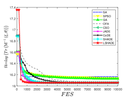
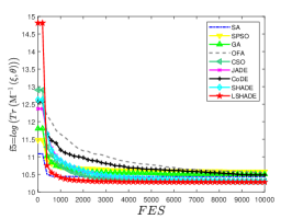
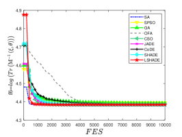
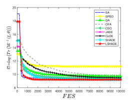
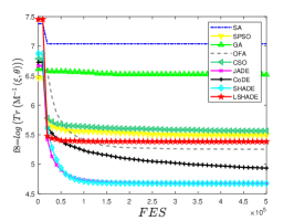
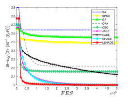
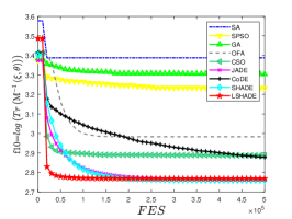
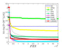
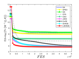
Figure 3: Mean Performance of the SA, SPSO, GA, OFA, CSO, JADE, CoDE, SHADE, and LSHADE algorithms for finding $A$-optimal designs.

4.3 Discussion

The LSHADE framework is used to generate the mutation vector with the “DE/current-to-pbest/1/bin” mutation strategy, and the parameter history update algorithm is used to adjust the adaptive parameters through the weighted Lehmer mean. Finally, the linear function is used to reduce the population scale gradually. In the repair process, since the number of support points is unknown, similar support points in the individual are combined with their corresponding weights along with very small weights from other support points. LSHADE performs very well for finding the $D$- and $A$-optimal design for many of the models in Table 1. However, in terms of convergence, the figures show LSHADE is inferior to JADE and SHADE for finding optimal designs for the 3-factor model in Problem 8, and the gamma regression model with 5 factors with pairwise interaction terms in Problem 11.

Table 10 reports the designs found by LSHADE under the $D$- and $A$-optimality criterion for Problems 1, 2 and 4-7. The table shows their support points and corresponding weights, the sensitivity function values at each of the support points and the efficiency lower bound of the generated design. For Problems 1, 2, 4-7, the LSHADE algorithm identifies the correct number of support points, which are 4, 6, 4, 3, 2 and 4, respectively. The efficiency lower bounds in Table 10 and the sensitivity plots in Figures 5 and 6 confirm the LSHADE-generated designs are either optimal or close to the optimum with a $D$ or $A$-efficiency of at least 95%.

Table 10: Designs generated by the LSHADE algorithm under the $D$-optimality and $A$-optimality criteria for Problem 1-2 and 4-7.

Problem	D-optimal design					A-optimal design
	X		W	S	D-efficiency lower bound	X		W	S	A-efficiency lower bound
1	0		0.25	0	1	0		0.0857	0.0074	0.9999
	0.3141		0.25	0		0.2723		0.1957	0.002
	1.1307		0.25	0		1.1827		0.2861	-0.0118
	2.7523		0.25	0		3		0.4325	0.0054
2	-1	0	0.1875	0	1	-1	0	0.1859	0.0001	0.9999
	-1	1	0.1875	0		-1	1	0.1399	-0.0003
	0	1	0.125	0		0	0	0.2287	0.0001
	0	0	0.125	0		0	1	0.1197	-0.0001
	1	1	0.1875	0		1	1	0.1399	0.0001
	1	0	0.1875	0		1	0	0.1859	0
4	0		0.25	0	1	0		0.1888	-1009.4201	0.9999
	0.3305		0.25	0		0.3011		0.3509	296.8851
	0.7692		0.25	0		0.7926		0.3119	-252.4479
	1		0.25	0		1		0.1484	1112.3723
5	0.2804	0	0.3333	0	1	0.2603	0	0.4785	-0.0007	0.9999
	3	0	0.3333	0		3	0	0.0595	0.0008
	3	0.7951	0.3333	0		3	0.826	0.462	0.0007
6	0.7143		0.5	0	1	0.5373		0.6696	0	1
	5		0.5	0		5		0.3304	0
7	3.1579	0	0.25	0	1	2.4402	0	0.2651	0.0001	0.9999
	4.0793	2.6754	0.25	0		3.3919	3.2516	0.3234	0.0016
	30	0	0.25	0		30	0	0.1398	-0.0003
	30	3.5789	0.25	0		30	4.7409	0.2717	-0.0018

Figure 4 and Figure 5 display, respectively, the sensitivity functions of the LSHADE-generated designs for Problem 1, 2, and 4-7 under the $D$- and $A$-optimality criteria. We omit sensitive functions which have larger dimensions because they become harder to appreciate graphically. In the figure, the red dots are support points generated by LSHADE and the all plots in Figure 4 confirm optimality of the designs found by LSHADE.

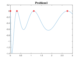
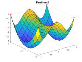
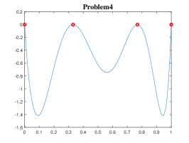
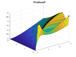
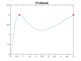
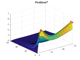
Figure 4: The sensitivity functions of the LSHADE-generated designs for Problems 1, 2, and 4-7 under the $D$-optimality criterion.

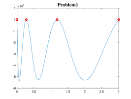
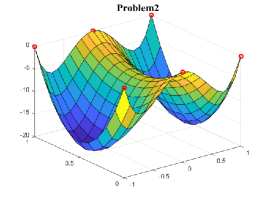
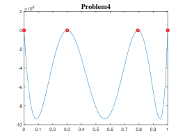
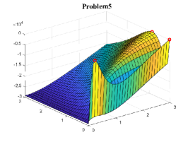
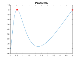
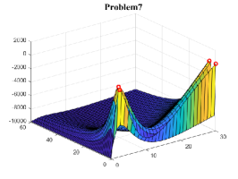
Figure 5: The sensitivity functions of the LSHADE-generated designs for Problems 1, 2, and 4-7 under the $A$-optimality criterion.

5 Conclusions

There are many evolutionary and nature-inspired metaheuristic algorithms for general optimization purposes. DE is one of the most well known evolutionary algorithms with many variants. A main goal in this study is to ascertain whether various EAs can find $D$- and $A$-optimal designs effectively for various types of statistical models in Table 1. Performance of several variants of DE for finding $D$- and $A$-optimal designs were compared using several measures and the LSHADE variant is the clear winner. In this paper, we propose the repair method to merge similar support points with their corresponding weights based on Euclidean distance and eliminate the corresponding support point with less weight to identify the number of the support points. To handle the infeasible weight solutions of individuals, the repair operation guarantees that the infeasible weight solutions on the $D$- and $A$-optimal design problems are fixed into the feasible weight solutions. To further enrich our optimal design experiment, our work utilizes DE variants to find $D$- and $A$-optimal experimental design. Among the compared algorithms, simulation experiments on 12 statistical models reveal that LSHADE achieves the best performance on the $D$- and $A$-optimal problems.

In the future work, we will aims at designing a better evolutionary algorithm for E-optimal design. Next we will construct the different types of optimal design criteria as the multi-objective optimal design problem and design the multi-objective evolutionary algorithm to trade off multi-objective optimal design problem.

References

- [1] B. Smucker, M. Krzywinski, N. Altman, Optimal experimental design, Nature methods 15 (8) (2018) 559–560.
- [2] A. C. Atkinson, The usefulness of optimum experimental designs, Journal of the Royal Statistical Society: Series B (Methodological) 58 (1) (1996) 59–76.
- [3] V. V. Fedorov, S. L. Leonov, Optimal design of dose response experiments: A model-oriented approach, Drug information journal: DIJ/Drug Information Association 35 (4) (2001) 1373–1383.
- [4] Z. Song, Z. Li, C. Yu, J. Hou, M. Wei, B. Bai, Y. Hu, D-optimal design for rapid assessment model of co2 flooding in high water cut oil reservoirs, Journal of Natural Gas Science and Engineering 21 (2014) 764–771.
- [5] K. Ogungbenro, A. Dokoumetzidis, L. Aarons, Application of optimal design methodologies in clinical pharmacology experiments, Pharmaceutical Statistics: The Journal of Applied Statistics in the Pharmaceutical Industry 8 (3) (2009) 239–252.
- [6] X. He, Laplacian regularized d-optimal design for active learning and its application to image retrieval, IEEE Transactions on Image Processing 19 (1) (2009) 254–263.
- [7] A. Atkinson, A. Donev, R. Tobias, Optimum experimental designs with SAS, Vol. 34, Oxford University Press, 2007.
- [8] V. V. Fedorov, Theory of optimal experiments, Elsevier, 2013.
- [9] F. Pukelsheim, B. Torsney, Optimal weights for experimental designs on linearly independent support points, The annals of Statistics (1991) 1614–1625.
- [10] W. K. Wong, Comparing robust properties of a, d, e and g-optimal designs, Computational statistics & data analysis 18 (4) (1994) 441–448.
- [11] R. García-Ródenas, J. C. García-García, J. López-Fidalgo, J. Á. Martín-Baos, W. K. Wong, A comparison of general-purpose optimization algorithms for finding optimal approximate experimental designs, Computational Statistics & Data Analysis 144 (2020) 106844.
- [12] Z. Stokes, A. Mandal, W. K. Wong, Using differential evolution to design optimal experiments, Chemometrics and Intelligent Laboratory Systems 199 (2020) 103955.
- [13] S. Kirkpatrick, C. D. Gelatt, M. P. Vecchi, Optimization by simulated annealing, science 220 (4598) (1983) 671–680.
- [14] V. Černỳ, Thermodynamical approach to the traveling salesman problem: An efficient simulation algorithm, Journal of optimization theory and applications 45 (1) (1985) 41–51.
- [15] J. H. Holland, et al., Adaptation in natural and artificial systems: an introductory analysis with applications to biology, control, and artificial intelligence, MIT press, 1992.
- [16] D. E. Goldberg, Genetic algorithms in search, Optimization, and MachineLearning.
- [17] J. Kennedy, R. Eberhart, Particle swarm optimization, in: Proceedings of ICNN’95-international conference on neural networks, Vol. 4, IEEE, 1995, pp. 1942–1948.
- [18] Z. Zhang, W. K. Wong, K. C. Tan, Competitive swarm optimizer with mutated agents for finding optimal designs for nonlinear regression models with multiple interacting factors, Memetic Computing 12 (3) (2020) 219–233.
- [19] R. Storn, K. Price, Differential evolution–a simple and efficient heuristic for global optimization over continuous spaces, Journal of global optimization 11 (4) (1997) 341–359.
- [20] J. Zhang, A. C. Sanderson, Jade: adaptive differential evolution with optional external archive, IEEE Transactions on evolutionary computation 13 (5) (2009) 945–958.
- [21] Y. Wang, Z. Cai, Q. Zhang, Differential evolution with composite trial vector generation strategies and control parameters, IEEE transactions on evolutionary computation 15 (1) (2011) 55–66.
- [22] R. Tanabe, A. Fukunaga, Success-history based parameter adaptation for differential evolution, in: 2013 IEEE congress on evolutionary computation, IEEE, 2013, pp. 71–78.
- [23] R. Tanabe, A. S. Fukunaga, Improving the search performance of shade using linear population size reduction, in: 2014 IEEE congress on evolutionary computation (CEC), IEEE, 2014, pp. 1658–1665.
- [24] J. Kiefer, General equivalence theory for optimum design (approximate theory), Annals of Statistics 2 (1974) 849–879.
- [25] A. Pázman, Foundations of optimum experimental design, Springer, 1986.
- [26] V. V. Fedorov, S. L. Leonov, Optimal design for nonlinear response models, CRC Press, 2013.
- [27] K. R. Opara, J. Arabas, Differential evolution: A survey of theoretical analyses, Swarm and evolutionary computation 44 (2019) 546–558.
- [28] H. Dette, V. B. Melas, W. K. Wong, Locally d-optimal designs for exponential regression models, Statistica Sinica (2006) 789–803.
- [29] H. Dette, V. B. Melas, et al., A note on the de la garza phenomenon for locally optimal designs, Annals of Statistics 39 (2) (2011) 1266–1281.
- [30] M. Yang, S. Biedermann, E. Tang, On optimal designs for nonlinear models: a general and efficient algorithm, Journal of the American Statistical Association 108 (504) (2013) 1411–1420.
- [31] M. E. Johnson, C. J. Nachtsheim, Some guidelines for constructing exact d-optimal designs on convex design spaces, Technometrics 25 (3) (1983) 271–277.
- [32] G. E. Box, W. G. Hunter, The experimental study of physical mechanisms, Technometrics 7 (1) (1965) 23–42.
- [33] J. López-Fidalgo, W. K. Wong, Design issues for the michaelis–menten model, Journal of Theoretical Biology 215 (1) (2002) 1–11.
- [34] B. Bogacka, M. Patan, P. J. Johnson, K. Youdim, A. C. Atkinson, Optimum design of experiments for enzyme inhibition kinetic models, Journal of Biopharmaceutical Statistics 21 (3) (2011) 555–572.
- [35] M. Zambrano-Bigiarini, M. Clerc, R. Rojas, Standard particle swarm optimisation 2011 at cec-2013: A baseline for future pso improvements, in: 2013 IEEE Congress on Evolutionary Computation, IEEE, 2013, pp. 2337–2344.
- [36] G.-Y. Zhu, W.-B. Zhang, Optimal foraging algorithm for global optimization, Applied Soft Computing 51 (2017) 294–313.
- [37] R. Cheng, Y. Jin, A competitive swarm optimizer for large scale optimization, IEEE transactions on cybernetics 45 (2) (2014) 191–204.